On the Sum-Capacity of Degraded Gaussian Multiaccess Relay Channels

Abstract

The sum-capacity is studied for a $K$-user degraded Gaussian multiaccess relay channel (MARC) where the multiaccess signal received at the destination from the $K$ sources and relay is a degraded version of the signal received at the relay from all sources, given the transmit signal at the relay. An outer bound on the capacity region is developed using cutset bounds. An achievable rate region is obtained for the decode-and-forward (DF) strategy. It is shown that for every choice of input distribution, the rate regions for the inner (DF) and outer bounds are given by the intersection of two $K$-dimensional polymatroids, one resulting from the multiaccess link at the relay and the other from that at the destination. Although the inner and outer bound rate regions are not identical in general, for both cases, a classical result on the intersection of two polymatroids is used to show that the intersection belongs to either the set of active cases or inactive cases, where the two bounds on the $K$-user sum-rate are active or inactive, respectively. It is shown that DF achieves the capacity region for a class of degraded Gaussian MARCs in which the relay has a high SNR link to the destination relative to the multiaccess link from the sources to the relay. Otherwise, DF is shown to achieve the sum-capacity for an active class of degraded Gaussian MARCs for which the DF sum-rate is maximized by a polymatroid intersection belonging to the set of active cases. This class is shown to include the class of symmetric Gaussian MARCs where all users transmit at the same power.

I Introduction

The multiaccess relay channel (MARC) is a network in which several users (sources) communicate with a single destination in the presence of a relay [1]. The coding strategies developed for the relay channel [2, 3] extend readily to the MARC [4, 5]. For example, the strategy of [3, theorem 1], now often called decode-and-forward (DF), has a relay that decodes user messages before forwarding them to the destination [4, 5]. Similarly, the strategy in [3, theorem 6], now often called compress-and-forward (CF), has the relay quantize its output symbols and transmit the resulting quantized bits to the destination [5].

Capacity results for relay channels are known only for a few special cases such as the class of degraded relay channels [3] and its multi-relay generalization [6, 7], the class of semi-deterministic relay channels [8], the class of orthogonal relay channels [9, 10], the class of Gaussian relay without delay channels [11, 12], and the class of ergodic phase-fading relay channels [4]. For the class of degraded relay channels, the degradedness condition requires that the received signal at the destination be independent of the source signal when conditioned on the transmit and receive signals at the relay. For the Gaussian case, this simplifies to the requirement that the signal received at the destination be a noisier version of that received at the relay conditioned on the transmitted signal at the relay. This condition immediately suggests that requiring the relay to decode the source signals should be optimal. In fact, for this class, applying this degradedness condition simplifies the cut-set outer bounds to coincide with the DF bounds. For the MARC, we generalize this degradedness condition to requiring that the signal received at the destination be independent of all source signals conditioned on the transmit and receive signals at the relay. Applying this degradedness condition to the cutset outer bounds for a MARC, however, does not simplify the bounds to those achieved by DF.

A $K$-user Gaussian MARC is degraded when the multiaccess signal received at the destination from the $K$ sources and relay is a noisier version of the signal received at the relay from all sources, given the transmit signal at the relay. For a $K$-user degraded Gaussian MARC, we develop the DF rate region as an inner bound on the capacity region using Gaussian signaling at the sources and relay. The outer bounds on the capacity region are obtained by specializing the cut-set bounds of [13, Th. 14.10.1] to the case of independent sources [14] and by applying the degradedness condition. In fact, for each choice of input distribution, both the DF and the cutset rate regions are intersections of two multiaccess rate regions, one with the relay as the receiver and the other with the destination as the receiver. In general, however, the inner and outer bounds differ in their input distributions as well as the rate bounds. The outer bounds allow a more general dependence between the source and relay signals relative to DF where we use auxiliary random variables, one for each source, to relate the transmitted signals at the sources and relay. For the Gaussian degraded MARC, we show that using Gaussian input signals at the sources and relay maximizes the outer bounds. For the inner bounds, we use Gaussian signaling at the sources and the relay via $K$ Gaussian auxiliary random variables. As a result, for each choice of the appropriate Gaussian input distribution, both the DF and outer bounds are then parametrized by $K$ source-relay cross-correlation coefficients, i.e., a $K$-length correlation vector. Specifically, each DF coefficient is a product of the two power fractions allocated for cooperation at the corresponding source and the relay, respectively. We show that the DF rate region over all feasible correlation vectors is a convex region. On the other hand, for the outer bounds, all the rate bounds at the relay except for the bound on the $K$-user sum-rate are non-concave functions of the correlation coefficients, and thus, the outer bound rate region requires time-sharing. Finally, we also show that for every feasible choice of the correlation vector, the multiaccess regions achieved by the inner and outer bounds at each receiver are polymatroids, and the resulting region is an intersection of two polymatroids.

We use a well-known result on the intersection of two polymatroids [15, chap. 46] to broadly classify polymatroid intersections into two categories, namely, the set of active and the set of inactive cases, depending on whether the constraints on the $K$-user sum-rate at both receivers are active or inactive, respectively. In fact, we use [15, chap. 46] to show that the $K$-user sum-rate for the inactive cases is always bounded by the minimum of the (inactive) $K$-user sum-rate bounds at each receiver, and thus, by the largest such bound. For both the inner and outer bounds, the intersection of the two rate polymatroids results in either an active or a inactive case for every choice of correlation vectors. In fact, the minimum of the $K$-user sum-rate bounds at the relay and destination is the effective sum-rate only if the polymatroid intersection is an active case and is strictly an upper bound for an inactive case.

Irrespective of the above mentioned distinction, we first consider the problem of maximizing the minimum of the $K$-user sum-rate bounds at the relay and destination over the set of all correlation coefficients. We solve this max-min optimization problem using techniques analogous to the classical minimax problem of detection theory [16, II.C]. We refer to a sum-rate optimal correlation vector as a max-min rule.

For both the inner and outer bounds, we show that the max-min optimization described above has two unique solutions. The first solution is given by the maximum $K$-user sum-rate achievable at the relay and results when the multiaccess link between the sources and the relay is the bottle-neck link. For this case, we show that the intersection of the rate regions at the relay and destination belongs to the set of active cases and is in fact the same as the region achieved at the relay. We further show that this region is the same for both the inner and outer bounds and is the capacity region for a class of degraded Gaussian MARCs where the source and relay powers satisfy the bottle-neck condition for this case.

The second solution pertains to the case in which the bottle-neck condition described above is not satisfied, i.e., the $K$-user sum-rate at the relay is at least as large as that at the destination. For this case, we show that for both the inner and outer bounds the max-min optimization solution requires the $K$-user sum-rate bounds at the relay and destination to be equal. In fact, we show that both the inner and outer bounds achieve the same maximum sum-rate for this case. Further, for both sets of bounds, we show that this maximum is achieved by a set of correlation vectors, i.e., the max-min rule is a set rather than a singleton. Recall, however, that the sum-rate computed thus is achievable for either bound only if there exists at least one max-min rule for which the polymatroid intersection belongs to the set of active cases; otherwise, the computed maximum is strictly an upper bound on the maximum sum-rate. Combining this with the fact that the maximum inner and outer $K$-user sum rate bounds for this case are the same, we establish that DF achieves the sum-capacity of an active class of degraded Gaussian MARCs, i.e., a class for which the maximum sum-rate is achieved because there exists at least one max-min rule for which the polymatroid intersection is an active case. We also show that the class of symmetric Gaussian MARCs, in which all sources have the same power, belongs to this active class. Finally, for the remaining inactive class of degraded Gaussian MARCs in which no active case results for any choice of the max-min rule, we provide a common upper bound on both the DF and the cutset sum-rates.

This paper is organized as follows. In Section II we present a model for a degraded Gaussian MARC. In Section III we develop the cut-set bounds on the capacity region of a MARC. In Section IV we determine the maximum $K$-user DF sum-rate. We discuss our results and conclude in Section V.

II Channel Model and Preliminaries

A $K$-user degraded Gaussian MARC has $K$ user (source) nodes, one relay node, and one destination node (see Fig. 1). The sources emit the messages $W_{k}$, $k=1,2,\ldots,K$, which are statistically independent and take on values uniformly in the sets $\{1,2,\ldots,M_{k}\}$. The channel is used $n$ times so that the rate of $W_{k}$ is $R_{k}=\left.B_{k}\right/n$ bits per channel use where $B_{k}=\log_{2}M_{k}$ bits. In each use of the channel, the input to the channel from source $k$ is $X_{k}$ while the relay’s input is $X_{r}$. The channel outputs $Y_{r}$ and $Y_{d}$, respectively, at the relay and the destination are

$$Y_{r} =\left(\sum\limits_{k=1}^{K}X_{k}\right)+Z_{r}$$ (1)

$$Y_{d} =\left(\sum\limits_{k=1}^{K}X_{k}\right)+X_{r}+Z_{d}$$ (2)

$$=Y_{r}+X_{r}+Z_{\Delta}$$ (3)

where $Z_{r}$ and $Z_{\Delta}$ are independent Gaussian random variables with zero means and variances $N_{r}$ and $N_{\Delta}$, respectively, such that the noise variance at the destination is

$$N_{d}=N_{r}+N_{\Delta}.$$ (4)

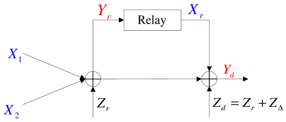
Figure 1: A two-user Gaussian degraded MARC.

We assume that the relay operates in a full-duplex manner, i.e., it can transmit and receive simultaneously in the same bandwidth. Further, its input $X_{r}$ in each channel use is a causal function of its outputs from previous channel uses. We write $\mathcal{K}=\{1,2,\ldots,K\}$ for the set of sources, $\mathcal{T}$ $=$ $\mathcal{K}$ $\cup$ $\{r\}$ for the set of transmitters, $\mathcal{R}$ $=$ $\{r,d\}$ for the set of receivers, $X_{\mathcal{S}}=\{X_{k}$ $:$ $k$ $\in$ $\mathcal{S}\}$ for all $\mathcal{S}$ $\subseteq$ $\mathcal{K}$, and $\mathcal{S}^{c}$ to denote the complement of $\mathcal{S}$ in $\mathcal{K}$.

The transmitted signals from source $k$ and the relay have a per symbol power constraint

$$\begin{array}[c]{cc}\left.E\left[\left|X_{k}\right|^{2}\right]\leq P_{k}\right.&\text{ }k\in\mathcal{T}.\end{array}$$ (5)

One can equivalently express the relationship between the input and output signals in (3) as a Markov chain

$$\left(X_{1},X_{2},\ldots,X_{K}\right)-(Y_{r},X_{r})-Y_{d}.$$ (6)

For $K$ $=$ $1$, (6) simplifies to the degradedness condition in [3, (10)] for the classic (single source) relay channel. A degraded Gaussian MARC is symmetric if $P_{k}=P$, for all $k$. Thus, a class of symmetric DG-MARCs is characterized by four parameters, namely, $P,$ $P_{r}\,,$ $N_{r},$ and $N_{d}$.

The capacity region $\mathcal{C}_{\text{MARC}}$ is the closure of the set of rate tuples $(R_{1},R_{2},\ldots,R_{K})$ for which the destination can, for sufficiently large $n$, decode the $K$ source messages with an arbitrarily small positive error probability. As further notation, we write $R_{\mathcal{S}}={\textstyle\sum\nolimits_{k\in\mathcal{S}}}R_{k}$ and $Y_{\mathcal{R}}=\left(Y_{r},Y_{d}\right)$. We write $\underline{0}$ and $\underline{1}$ to denote vectors whose entries are all zero and one, respectively, and $C(x)=\log(1+x)/2$ to denote the capacity of an AWGN channel with signal-to-noise ratio (SNR) $x$. We use the usual notation for entropy and mutual information [17, 13] and take all logarithms to the base 2 so that in each channel use our rate units are bits.

III Outer Bounds

An outer bound on the capacity region of a MARC is presented in [14] using the cut-set bounds in [13, Th. 14.10.1] as applied to the case of independent sources. We summarize the bounds below.

Proposition 1

The capacity region $\mathcal{C}_{\text{MARC}}$ is contained in the union of the set of rate tuples $(R_{1},R_{2},\ldots,R_{K})$ that satisfy, for all $\mathcal{S}\subseteq\mathcal{K}$,

$$R_{\mathcal{S}}\leq\min\left\{I(X_{\mathcal{S}};Y_{r},Y_{d}|X_{\mathcal{S}^{c}},X_{r},U),I(X_{\mathcal{S}},X_{r};Y_{d}|X_{\mathcal{S}^{c}},U)\right\}$$ (7)

where the union is over all distributions that factor as

$$p(u)\cdot\left(\prod\nolimits_{k=1}^{K}p(x_{k}|u)\allowbreak\right)\cdot p(x_{r}|\allowbreak x_{\mathcal{K}}\allowbreak,u)\cdot p(y_{r},y_{d}|x_{\mathcal{K}},x_{r}).$$ (8)

Remark 1

The time-sharing random variable $U$ ensures that the region in (7) is convex. One can apply Caratheodory’s theorem [18] to this $K$-dimensional convex region to bound the cardinality of $U$ as $\left|\mathcal{U}\right|\leq K+1$.

Consider the outer bounds in Proposition 1. For a degraded Gaussian MARC applying the degradness definition in (6) simplifies (7) as

$$\begin{array}[c]{cc}R_{\mathcal{S}}\leq\min\left\{I(X_{\mathcal{S}};Y_{r}|X_{r}X_{\mathcal{S}^{c}}U),I(X_{\mathcal{S}}X_{r};Y_{d}|X_{\mathcal{S}^{c}}U)\right\}&\text{for all }\mathcal{S}\subseteq\mathcal{K}\end{array}$$ (9)

for the same joint distribution in (8). In the following theorem, we develop the bounds in (9) with $U$ as a constant. For notational convenience, for a constant $U$, we write $B_{r,\mathcal{S}}$ and $B_{d,\mathcal{S}}$ to denote the first and second terms, respectively, of the minimum on the right-side of (9). The proof of the following theorem is detailed in Appendix A.

Theorem 1

For a degraded Gaussian MARC, the bounds $B_{r,\mathcal{S}}$ and $B_{d,\mathcal{S}}$ are given by

$$B_{r,\mathcal{S}}=\left\{\begin{array}[c]{ll}C\left({\textstyle\sum\limits_{k\in\mathcal{S}}}\frac{P_{k}}{N_{r}}\right)&{\textstyle\sum\limits_{k\in\mathcal{S}^{c}}}\gamma_{k}=1\\ C\left({\textstyle\sum\limits_{k\in\mathcal{S}}}\frac{P_{k}}{N_{r}}-\frac{\left(\sum\limits_{k\in\mathcal{S}}\sqrt{\gamma_{k}P_{k}}\right)^{2}}{N_{r}\overline{\gamma}_{\mathcal{S}^{c}}}\right)&\text{otherwise}\end{array}\right.$$ (10)

and

$$B_{d,\mathcal{S}}=C\left(\frac{{\textstyle\sum\limits_{k\in\mathcal{S}}}P_{k}+\overline{\gamma}_{\mathcal{S}^{c}}P_{r}+2{\textstyle\sum\limits_{k\in\mathcal{S}}}\sqrt{\gamma_{k}P_{k}P_{r}}}{N_{d}}\right)$$ (11)

where $\overline{\gamma}_{\mathcal{S}^{c}}=1-\sum_{k\in\mathcal{S}^{c}}\gamma_{k}$ and

$$\begin{array}[c]{cc}\sqrt{\gamma_{k}P_{k}P_{r}}\overset{\vartriangle}{=}E(X_{k}X_{r})&\text{for all }k\in\mathcal{K}.\end{array}$$ (12)

Remark 2

For $K$ $=$ $1$, the bounds in (10) and (11) simplify to the first and second bound, respectively, for the degraded relay channel in [3, theorem 5].

Remark 3

The source-relay cross-correlation variables $\gamma_{k}$, for all $k$, satisfy (111), i.e., they lie in the closed convex region $\Gamma_{OB}$ given by

$$\Gamma_{OB}=\left\{\underline{\gamma}_{\mathcal{K}}:\sum_{k\in\mathcal{K}}\gamma_{k}\leq 1\right\}.$$ (13)

The bound $B_{r,\mathcal{S}}$ in (10), in general, is not a concave function of $\underline{\gamma}_{\mathcal{K}}$ for any $\mathcal{S}\subset\mathcal{K}$. For a fixed $\underline{\gamma}_{\mathcal{S}^{c}}$, in Appendix D we show that $B_{r,\mathcal{S}}$ is a concave function of $\underline{\gamma}_{\mathcal{S}}$. This in turn implies that $B_{r,\mathcal{K}}$ is a concave function of $\underline{\gamma}_{\mathcal{K}}$. Further, in Appendix C we show that for all $\mathcal{S}$, $B_{d,\mathcal{S}}$ in (11) is a concave function of $\underline{\gamma}_{\mathcal{K}}$.

Remark 4

In the expression for $B_{d,\mathcal{S}}$ in (11), the terms involving the cross-correlation coefficients quantify the coherent combining gains that result from choosing correlated source and relay signals. On the other hand, the expression for $B_{r,\mathcal{S}}$ in (10) quantifies the upper bounds on the rate achievable at the relay when one or more source signals are correlated with the transmitted signal at the relay.

The rate region $\mathcal{R}_{OB}$ enclosed by the cut-set outer bounds is obtained as follows. From (125) for any choice of $\underline{\gamma}_{\mathcal{K}}$, the rate region is an intersection of the regions enclosed by the bounds $B_{r,\mathcal{S}}$ and $B_{d,\mathcal{S}}$ for all $\mathcal{S}$. Since $B_{r,\mathcal{S}}$ is not a concave function of $\underline{\gamma}_{\mathcal{K}}$, one must also consider all possible convex combinations of $\underline{\gamma}_{\mathcal{K}}$ to obtain $\mathcal{R}_{OB}$. For the $K$-dimensional convex region $\mathcal{R}_{OB}$, one can apply Caratheodory’s theorem [18] to express every rate tuple $(R_{1},R_{2},\ldots,R_{K})$ in $\mathcal{R}_{OB}$ as a convex combination of at most $K+1$ rate tuples, where each rate tuple is obtained for a specific choice of $\underline{\gamma}_{\mathcal{K}}$. Let $\Theta$ denote the collection of all vectors $\eta$ that satisfy

$${\textstyle\sum\nolimits_{m=1}^{K+1}}\eta_{m}=1$$ (14)

and let $\underline{\zeta}\equiv(\{\underline{\gamma}_{\mathcal{K}}\}_{K+1},$$\eta$$)\in\Gamma_{OB}^{K+1}\times\Theta$ denote a collection of $K+1$ power fractions and weights such that the rate tuple achieved by the $m^{th}$ vector $\underline{\gamma}_{\mathcal{K}}^{(m)}$ is weighted by the $m^{th}$ non-negative entry of the weight vector $\eta$, for all $m\in\mathcal{K\cup}\left\{K+1\right\}$. Finally, since $\Gamma_{OB}$ in (13) is a closed convex set, ${\textstyle\sum\nolimits_{m=1}^{K+1}}\eta_{m}\underline{\gamma}_{\mathcal{K}}^{(m)}\in\Gamma_{OB}$. The following theorem presents an outer bound on the capacity region of the degraded Gaussian MARC.

Theorem 2

The capacity region $\mathcal{C}_{\text{MARC }}$of a degraded Gaussian MARC is contained in the region $\mathcal{R}_{OB}$ given as

$$\mathcal{R}_{OB}=\bigcup\limits_{\underline{\zeta}\in\Gamma_{OB}}\left(\mathcal{R}_{r}^{ob}\left(\underline{\zeta}\right)\cap\mathcal{R}_{d}^{ob}\left(\underline{\zeta}\right)\right)$$ (15)

where the rate region $\mathcal{R}_{j}^{ob}\left(\underline{\zeta}\right)$, $j=r,d$, is

$$\mathcal{R}_{j}^{ob}\left(\underline{\zeta}\right)=\left\{\left(R_{1},R_{2},\ldots,R_{K}\right):0\leq R_{\mathcal{S}}\leq\overline{B}_{j,\mathcal{S}}\left(\underline{\zeta}\right)\right\}$$ (16)

and the bound $\overline{B}_{j,\mathcal{S}}$ is given by

$$\overline{B}_{j,\mathcal{S}}\left(\underline{\zeta}\right)=\sum\limits_{m=1}^{K+1}\eta_{m}B_{j,\mathcal{S}}\left(\underline{\gamma}_{\mathcal{K}}^{(m)}\right).$$ (17)

Theorem 3

The regions $\mathcal{R}_{r}^{ob}\left(\underline{\zeta}\right)$ and $\mathcal{R}_{d}^{ob}\left(\underline{\zeta}\right)$ are polymatroids.

Proof:

In Appendix B we show that for each choice of input distribution satisfying (8), the bounds in (54) are submodular set functions, i.e., they enclose regions that are polymatroids. For the optimal Gaussian input distribution, this implies that $\mathcal{R}_{r}^{ob}\left(\underline{\zeta}\right)$ and $\mathcal{R}_{d}^{ob}\left(\underline{\zeta}\right)$ are polymatroids for every choice of $\underline{\zeta}$. ∎

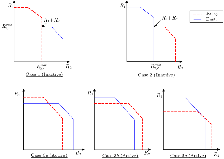
Figure 2: Five possible intersections of $\mathcal{R}_{r}$ and $\mathcal{R}_{d}$ for a two-user Gaussian MARC.

The region $\mathcal{R}_{OB}$ in (66) is a union of the intersections of the regions $\mathcal{R}_{r}^{ob}$ and $\mathcal{R}_{d}^{ob}$, where the union is taken over all convex combinations of $\underline{\gamma}_{\mathcal{K}}$. Since $\mathcal{R}_{OB}$ is convex, we obtain the boundary of $\mathcal{R}_{OB}$ by maximizing the weighted sum ${\textstyle\sum\nolimits_{k\in\mathcal{K}}}\mu_{k}R_{k}$ over all $\Gamma_{OB}$ and for all $\mu_{k}>0$. Specifically, we determine the sum-rate $R_{\mathcal{K}}$ when $\mu_{k}$ $=$ $1$ for all $k$. In general, to determine the intersecting polytope, one has to consider all possible polytope shapes for the regions $\mathcal{R}_{r}^{ob}$ and $\mathcal{R}_{d}^{ob}$. However, since $\mathcal{R}_{r}^{ob}$ and $\mathcal{R}_{d}^{ob}$ are polymatroids, we use the following lemma on polymatroid intersections [15, p. 796, Cor. 46.1c] to broadly classify the intersection of two polymatroids into two categories. The first inactive set category includes all intersections for which the constraints on the two $K$-user sum-rates are not active. This implies that no rate tuple on the sum-rate plane achieved at one of the receivers lies within or on the boundary of the rate region achieved at the other receiver. On the other hand, the intersections for which there exists at least one such rate tuple, i.e., the constraints on the two $K$-user sum-rates are active in the final intersection, belong to the category of active set. In Fig. 2, for a two-user MARC we illustrate the five possible choices for the sum-rate resulting from an intersection of $\mathcal{R}_{r}^{ob}(\underline{\gamma}_{\mathcal{K}})$ and $\mathcal{R}_{d}^{ob}(\underline{\gamma}_{\mathcal{K}})$. Cases $1$ and $2$ belong to the inactive set while cases $3a,$ $3b$, and $3c$ belong to the active set. We henceforth refer to members of the active and the inactive sets as active and inactive cases, respectively. Note that Fig. 2 illustrates two specific $\mathcal{R}_{r}^{ob}$ and $\mathcal{R}_{d}^{ob}$ polymatroids for cases $3a$, $3b$, and $3c$. In general the active set includes all intersections that satisfy the definition for this set including cases such as $\mathcal{R}_{r}^{ob}\subseteq\mathcal{R}_{d}^{ob}$ and vice-versa. Finally, note that the sum-rate is a minimum of the sum-rates at the two receivers only for the active cases $3a$, $3b$, and $3c$. For the inactive cases $1$ and $2$, the $R_{1}+R_{2}$ constraints are no longer active and the sum-rate is given by the bounds $\overline{B}_{r,\{2\}}+\overline{B}_{d,\{1\}}$ and $\overline{B}_{r,\{2\}}+\overline{B}_{d,\{1\}}$, respectively. We use the following lemma on polymatroid intersections to generalize this observation and develop an outer bound on the $K$-user sum-rate.

Lemma 1

Let $R_{\mathcal{S}}\leq f_{1}\left(\mathcal{S}\right)$ and $R_{\mathcal{S}}\leq f_{2}\left(\mathcal{S}\right)$, for all $\mathcal{S}\subseteq\mathcal{K}$, be two polymatroids such that $f_{1}$ and $f_{2}$ are nondecreasing submodular set functions on $\mathcal{K}$ with $f_{1}\left(\emptyset\right)=f_{2}\left(\emptyset\right)=0$. Then

$$\max R_{\mathcal{K}}=\min\limits_{\mathcal{S}\subseteq\mathcal{K}}\left(f_{1}\left(\mathcal{S}\right)+f_{2}\left(\mathcal{K}\backslash\mathcal{S}\right)\right).$$ (18)

From Lemma 1 we see that the maximum $K$-user sum-rate $R_{\mathcal{K}}$ that results from the intersection of two polymatroids, $R_{\mathcal{S}}\leq f_{1}\left(\mathcal{S}\right)$ and $R_{\mathcal{S}}\leq f_{2}\left(\mathcal{S}\right)$ is given by the minimum of the two $K$-user sum-rate planes $f_{1}\left(\mathcal{K}\right)$ and $f_{2}\left(\mathcal{K}\right)$ only if both the sum-rates are at most as large as the sum of the orthogonal rate planes $f_{1}\left(\mathcal{S}\right)$ and $f_{2}\left(\mathcal{K}\backslash\mathcal{S}\right)$, for all $\emptyset\not=\mathcal{S}\subset\mathcal{K}$. Further, the resulting intersection belongs to the set of active cases. Conversely, when there exists at least one $\emptyset\not=\mathcal{S}\subset\mathcal{K}$ for which the above condition is not true, an inactive case results. Physically, an inactive case results when a subset $\mathcal{S}$ of all users achieve better rates at one of the receivers while the remaining subset of users achieve a better rate at the other receiver. For such inactive cases, the maximum sum-rate in (18) is the sum of two orthogonal rate planes achieved by the two complementary subsets of users. As a result, the $K$-user sum-rate bounds $f_{1}(\mathcal{K})$ and $f_{2}(\mathcal{K})$ are no longer active for this case, and thus, the region of intersection is no longer a polymatroid with $2^{K}-1$ faces.

In the following theorem we use Lemma 1 to develop the upper bound on the $K$-user sum-rate. For a Gaussian input distribution, the polymatroids $\mathcal{R}_{r}^{ob}$ and $\mathcal{R}_{d}^{ob}$ are parametrized by $\underline{\zeta}$, and thus, Lemma 1 applies for each choice of $\underline{\zeta}$.

Theorem 4

For each $\underline{\zeta}\in\Gamma_{OB}$, the maximum $K$-user sum-rate $R_{\mathcal{K}}$ resulting from the intersecting polymatroids $\mathcal{R}_{r}^{ob}$ and $\mathcal{R}_{d}^{ob}$ is

$$R_{\mathcal{K}}=\left\{\begin{array}[c]{ll}\overline{B}_{d,\mathcal{A}}+\overline{B}_{r,\mathcal{A}^{c}}&\text{condition }1\text{ }\\ \min\left(\overline{B}_{r,\mathcal{K}},\overline{B}_{d,\mathcal{K}}\right)&\text{otherwise}\end{array}\right.$$ (19)

where $\overline{B}_{d,\mathcal{S}}$ and $\overline{B}_{r,\mathcal{S}}$ for all $\mathcal{S}$ are functions of $\underline{\zeta}_{\mathcal{K}}$ and condition $1$ is defined for any $\emptyset\not=\mathcal{A\subset K}$ as

$$\overline{B}_{d,\mathcal{A}}+\overline{B}_{r,\mathcal{A}^{c}}<\min\left(\overline{B}_{r,\mathcal{K}},\overline{B}_{d,\mathcal{K}}\right).$$ (20)

Remark 5

The condition in (20) determines whether the intersection of two polymatroids belongs to either the set of active or the set of inactive cases with respect to the $K$-user sum-rate.

Proof:

The proof follows from applying Lemma 1 to the maximization of $R_{\mathcal{K}}$ for each choice of $\underline{\zeta}$. ∎

For a fixed transmit power $P_{k}$, for all $k\in\mathcal{T}$, and noise variances $N_{r}$ and $N_{d}$, the choice of $\underline{\zeta}$ determines whether the intersection of $\mathcal{R}_{r}^{ob}\left(\underline{\zeta}\right)$ and $\mathcal{R}_{d}^{ob}\left(\underline{\zeta}\right)$ belongs to the set of active or inactive cases. For each choice of $\underline{\zeta}$, from Theorem 4 an active case results only if for all $2^{K}-1$ non-empty subsets $\mathcal{A}$ of $\mathcal{K}$, the condition in (20) does not hold. Further, for any $\underline{\zeta}$ that results in an inactive case, from Theorem 4, the sum-rate is bounded as

$$\overline{B}_{d,\mathcal{A}}+\overline{B}_{r,\mathcal{A}^{c}}<\min\left(\overline{B}_{r,\mathcal{K}},\overline{B}_{d,\mathcal{K}}\right)<\max_{\underline{\zeta}\in\Gamma_{OB}}\min\left(\overline{B}_{r,\mathcal{K}},\overline{B}_{d,\mathcal{K}}\right).$$ (21)

To this end, we consider the optimization problem

$$R_{\mathcal{K}}=\max\limits_{\underline{\zeta}\in\Gamma_{OB}}\min\left(\overline{B}_{r,\mathcal{K}}\left(\underline{\zeta}\right),\overline{B}_{d,\mathcal{K}}\left(\underline{\zeta}\right)\right).$$ (22)

In general, optimizing non-convex functions is not straightforward. However, since $B_{r,\mathcal{K}}$ and $B_{d,\mathcal{K}}$ are concave functions of $\underline{\gamma}_{\mathcal{K}}$, the above max-min optimization simplifies to

$$R_{\mathcal{K}}=\max\limits_{\underline{\gamma}_{\mathcal{K}}\in\Gamma_{OB}}\min\left\{B_{r,\mathcal{K}}\left(\underline{\gamma}_{\mathcal{K}}\right),B_{d,\mathcal{K}}\left(\underline{\gamma}_{\mathcal{K}}\right)\right\}.$$ (23)

Note that the optimization is performed over the same set in (22) and (23) as $\Gamma_{OB}$ is a closed convex set. In Appendix E, we show that the max-min problem in (23) is a dual of the classical minimax problem of detection theory, (see for e.g., [16, II.C]). This allows us to apply the techniques used to obtain a minimax solution to maximize the bounds in (23) over all $\underline{\gamma}_{\mathcal{K}}$ in $\Gamma_{OB}$ (see also [9]). We write $\underline{\gamma}_{\mathcal{K}}^{\ast}$ to denote a sum-rate optimal allocation, i.e., a max-min rule, and write $\mathcal{G}$ to denote the set of all $\underline{\gamma}_{\mathcal{K}}^{\ast}$ maximizing (23). A general solution to the max-min optimization in (23) simplifies to three cases [16, II.C]. The first two correspond to those in which the maximum achieved by one of the two functions is smaller than the other, while the third corresponds to the case in which the maximum results when the two functions are equal (see Fig. 4). For $B_{r,\mathcal{K}}$ and $B_{d,\mathcal{K}}$ defined in (10) and (11), respectively, we now show that the solution simplifies to the consideration of only two cases. The following theorem summarizes the solution to the max-min problem in (23). The proof is developed in Appendix E.

Theorem 5

The max-min optimization

$$R_{\mathcal{K}}=\max\limits_{\underline{\gamma}_{\mathcal{K}}\in\Gamma_{OB}}\min\left\{B_{r,\mathcal{K}}\left(\underline{\gamma}_{\mathcal{K}}\right),B_{d,\mathcal{K}}\left(\underline{\gamma}_{\mathcal{K}}\right)\right\}$$ (24)

simplifies to the following two cases.

$$\begin{array}[c]{lll}\text{Case }1\text{:}&R_{\mathcal{K}}=C\left(\frac{{\textstyle\sum\limits_{k\in\mathcal{K}}}P_{k}}{N_{r}}\right),&B_{r,\mathcal{K}}\left(\underline{0}\right)<B_{d,\mathcal{K}}\left(\underline{0}\right)\\ \text{Case }2\text{:}&R_{\mathcal{K}}=C\left(\left({\textstyle\sum\limits_{k\in\mathcal{K}}}\frac{P_{k}}{N_{r}}\right)-\frac{\left(x^{\ast}\right)^{2}P_{\max}}{N_{r}}\right)\equiv B^{\ast},&B_{r,\mathcal{K}}^{\ast}\left(\underline{\gamma}_{\mathcal{K}}^{\ast}\right)=B_{d,\mathcal{K}}^{\ast}\left(\underline{\gamma}_{\mathcal{K}}^{\ast}\right)\end{array}$$ (25)

where $P_{\max}=\max_{k\in\mathcal{K}}P_{k}$, $\lambda_{k}\overset{\vartriangle}{=}P_{k}/P_{\max}$, and $x^{\ast}\overset{\vartriangle}{=}\sum_{k\in\mathcal{K}}\sqrt{\lambda_{k}\gamma_{k}^{\ast}}$ is the unique solution satisfying $B_{r.\mathcal{K}}\left(\underline{\gamma}_{\mathcal{K}}^{\ast}\right)=B_{r.\mathcal{K}}\left(\underline{\gamma}_{\mathcal{K}}^{\ast}\right)$ and is given by

$$x^{\ast}=\frac{-K_{1}+\sqrt{K_{1}^{2}+\left(K_{3}-K_{2}\right)K_{0}}}{K_{0}}$$ (26)

with

$$\begin{array}[c]{ll}K_{0}=P_{\max}\left/N_{r}\right.,&K_{1}=\sqrt{P_{\max}P_{r}}\left/N_{d}\right.\\ K_{2}=\frac{\sum\nolimits_{k\in\mathcal{K}}P_{k}}{N_{d}}+\frac{P_{r}}{N_{d}},\text{ and}&K_{3}=\frac{{\textstyle\sum\nolimits_{k\in\mathcal{K}}}P_{k}}{N_{r}}.\end{array}$$ (27)

Remark 6

The maximization in (24) is independent of whether the optimal $\underline{\gamma}_{\mathcal{K}}^{\ast}$ results in an active or an inactive case. However, not all max-min rules $\underline{\gamma}_{\mathcal{K}}^{\ast}\in\mathcal{G}$ will result in an active case. In general, active cases may be achieved only by a subset $\mathcal{G}_{a}$ $\subseteq\mathcal{G}$. However, irrespective of the kind of intersection, from Lemma 1, (25) is an upper bound on the $K$-user sum-rate cutset bounds.

In the following theorem we show that it suffices to consider two conditions in determining the largest outer bound on the $K$-user sum-capacity. We enumerate the two conditions as

$$\begin{array}[c]{cc}\text{Condition 1:}&B_{r,\mathcal{K}}(\underline{0})\leq B_{d,\mathcal{K}}(\underline{0})\\ \text{Condition 2:}&B_{r,\mathcal{K}}(\underline{0})>B_{d,\mathcal{K}}(\underline{0}).\end{array}$$ (28)

The first condition implies that the maximum $K$-user cutset bound at the relay is smaller than the corresponding bound at the destination; for this case, we show that $B_{r,\mathcal{S}}(\underline{0})<B_{d,\mathcal{S}}(\underline{0})$ for all $\mathcal{S}\subset\mathcal{K}$, i.e., $\mathcal{R}_{OB}=\mathcal{R}_{r}^{ob}\subset\mathcal{R}_{d}^{ob}$. On the other hand, when condition 2 occurs, i.e., when condition 1 does not hold in (28), we use the monotone properties of $B_{r,\mathcal{K}}$ and $B_{d,\mathcal{K}}$ and Lemma 1 to show that

$$R_{K}\leq\max\limits_{\underline{\gamma}_{\mathcal{K}}\in\Gamma_{OB}}\min\left\{B_{r,\mathcal{K}}\left(\underline{\gamma}_{\mathcal{K}}\right),B_{d,\mathcal{K}}\left(\underline{\gamma}_{\mathcal{K}}\right)\right\}$$ (29)

with equality achieved in (29) when the polymatroid intersection is an active case. From Theorem 5 we have that a continuous set, $\mathcal{G}$, of $\underline{\gamma}_{\mathcal{K}}^{\ast}$ maximizes the right-hand-side of (29). We show that the bound in (29) is achieved with equality when there exists a $\underline{\gamma}_{\mathcal{K}}^{\ast}$ that results in an active case, i.e., in a non-empty $\mathcal{G}_{a}$. Finally, for the class of symmetric degraded G-MARCs, we prove the existence of an active case that maximizes the sum-rate.

Theorem 6

The largest outer bound $R_{\mathcal{K}}^{ob}$ on the $K$-user sum-rate is

$$\begin{array}[c]{ll}R_{\mathcal{K}}^{ob}=C\left(\sum_{k\in\mathcal{K}}P_{k}/N_{r}\right),&\text{if }B_{r,\mathcal{K}}(\underline{0})<B_{d,\mathcal{K}}(\underline{0})\\ R_{\mathcal{K}}^{ob}\leq C\left(\left({\textstyle\sum\limits_{k\in\mathcal{K}}}\frac{P_{k}}{N_{r}}\right)-\frac{\left(x^{\ast}\right)^{2}P_{\max}}{N_{r}}\right),&\text{otherwise}\end{array}$$ (30)

where $x^{\ast}\overset{\vartriangle}{=}\sum_{k\in\mathcal{K}}\sqrt{\lambda_{k}\gamma_{k}^{\ast}}$ is the unique solution satisfying $B_{r,\mathcal{K}}(\underline{\gamma}^{\ast})=B_{d,\mathcal{K}}(\underline{\gamma}^{\ast})$ and is given by (26) and (27). The bound in (30) is achieved with equality only when the intersection of $\mathcal{R}_{r}^{ob}(\underline{\gamma}_{\mathcal{K}}^{\ast})$ and $\mathcal{R}_{d}^{ob}(\underline{\gamma}_{\mathcal{K}}^{\ast})$ results in an active case. The bound is achieved with equality for the class of symmetric degraded G-MARCs.

Proof:

Let $\underline{\gamma}_{\mathcal{K}}=\underline{0}$. From (10) we see that $B_{\mathcal{S},r}(\underline{\gamma}_{\mathcal{S}}\not=\underline{0})<B_{\mathcal{S},r}(\underline{0})$, for all $\mathcal{S}\subseteq\mathcal{K}$, i.e, the region $\mathcal{R}_{r}^{(ob)}(\underline{\gamma}_{\mathcal{K}})$ is largest at $\underline{\gamma}_{\mathcal{K}}=\underline{0}$. Expanding $B_{\mathcal{S},r}$ and $B_{\mathcal{S},d}$ at $\underline{\gamma}_{\mathcal{K}}=\underline{0}$ from (10) and (11), respectively, we have

$$B_{r,\mathcal{S}}\left(\underline{0}\right) =C\left(\frac{\sum_{k\in\mathcal{S}}P_{k}}{N_{r}}\right)$$ (31)

$$B_{d,\mathcal{S}}\left(\underline{0}\right) =C\left(\frac{\sum_{k\in\mathcal{S}}P_{k}}{N_{d}}+\frac{P_{r}}{N_{d}}\right).$$ (32)

The sum-rate resulting from the intersection of $\mathcal{R}_{r}^{ob}\left(\underline{0}\right)$ and $\mathcal{R}_{d}^{ob}\left(\underline{0}\right)$ falls into one of following two cases.

Case 1: The first case results when $B_{\mathcal{K},r}\left(\underline{0}\right)\leq B_{\mathcal{K},d}\left(\underline{0}\right)$. From (31) and (32) this condition simplifies to

$$\frac{\sum\limits_{k\in\mathcal{K}}P_{k}}{N_{r}}\leq\frac{\sum\limits_{k\in\mathcal{K}}P_{k}}{N_{d}}+\frac{P_{r}}{N_{d}}.$$ (33)

Expanding (33), we have, for any $\mathcal{S\subset K}$,

$$\frac{{\textstyle\sum\limits_{k\in\mathcal{S}}}P_{k}}{N_{r}} \leq\frac{{\textstyle\sum\limits_{k\in\mathcal{S}}}P_{k}+P_{r}}{N_{d}}-\frac{{\textstyle\sum\limits_{k\in\mathcal{S}^{c}}}P_{k}\left(N_{d}-N_{r}\right)}{N_{d}N_{r}}$$ (34)

$$<\frac{{\textstyle\sum\limits_{k\in\mathcal{S}}}P_{k}+P_{r}}{N_{d}}$$ (35)

where (35) follows from the degradedness condition in (4). Thus, $B_{r,\mathcal{K}}(\underline{0})\leq B_{d,\mathcal{K}}(\underline{0})$ implies that $B_{r,\mathcal{S}}(\underline{0})<B_{d,\mathcal{S}}(\underline{0})$ for all $\mathcal{S}\subset\mathcal{K}$, i.e., $\mathcal{R}_{r}^{ob}(\underline{0})\subset\mathcal{R}_{d}^{ob}(\underline{0})$, and $\mathcal{R}_{OB}(\underline{0})=\mathcal{R}_{r}^{ob}(\underline{0})$. The maximum $K$-user sum-rate upper bound for this active case is then

$$R_{\mathcal{K}}^{ob}=B_{r,\mathcal{K}}=C({\textstyle\sum\nolimits_{k\in\mathcal{K}}}P_{k}\left/N_{r}\right.).$$ (36)

Case 2: The second case results when $B_{\mathcal{K},r}\left(\underline{0}\right)>B_{\mathcal{K},d}\left(\underline{0}\right),$ i.e., when

$$\frac{\sum\limits_{k\in\mathcal{K}}P_{k}}{N_{r}}>\frac{\sum\limits_{k\in\mathcal{K}}P_{k}}{N_{d}}+\frac{P_{r}}{N_{d}}.$$ (37)

Unlike case $1$, (37) does not imply that $B_{\mathcal{S},r}\left(\underline{0}\right)>B_{\mathcal{S},d}\left(\underline{0}\right)$ or vice-versa, for all $\mathcal{S}\subset\mathcal{K}$. From Theorem 4, the intersection of $\mathcal{R}_{r}^{ob}\left(\underline{0}\right)$ and $\mathcal{R}_{d}^{ob}\left(\underline{0}\right)$ can result in either an active or an inactive case and thus, from (20), we have

$$R_{\mathcal{K}}^{ob}\leq\min(B_{r,\mathcal{K}}\left(\underline{0}\right),B_{d,\mathcal{K}}\left(\underline{0}\right))=B_{d,\mathcal{K}}\left(\underline{0}\right)$$ (38)

with equality for the active case. Note that from symmetry an active case results for the symmetric G-MARC. We now show that the sum-rate is increased for a $\underline{\gamma}_{\mathcal{K}}^{\ast}\not=\underline{0}$ such that $B_{r,\mathcal{K}}\left(\underline{\gamma}_{\mathcal{K}}^{\ast}\right)=B_{d,\mathcal{K}}\left(\underline{\gamma}_{\mathcal{K}}^{\ast}\right)$. To simplify the exposition, we write $B_{r,\mathcal{K}}$ and $B_{d,\mathcal{K}}$ in (10) and (11) as

$$B_{r,\mathcal{K}}\left(x\right) =C\left(\frac{{\textstyle\sum\limits_{k\in\mathcal{K}}}P_{k}}{N_{r}}-\frac{x^{2}P_{\max}}{N_{r}}\right)$$ (39)

$$B_{d,\mathcal{K}}\left(x\right) =C\left(\frac{{\textstyle\sum\limits_{k\in\mathcal{K}}}P_{k}}{N_{d}}+\frac{P_{r}}{N_{d}}+\frac{2x\sqrt{P_{\max}P_{r}}}{N_{d}}\right)$$ (40)

where

$$x\overset{\vartriangle}{=}\sum_{k=1}^{K}\sqrt{\gamma_{k}\lambda_{k}}$$ (41)

and $\lambda_{k}=P_{k}/P_{\max}$ where $P_{\max}=\max_{k\in\mathcal{K}}P_{k}$, for all $k$. For all $\gamma_{k}\in[0,1]$, we have

$$\begin{array}[c]{cc}\frac{\partial x}{\partial\gamma_{k}}=\frac{\sqrt{\lambda_{k}}}{2\sqrt{\gamma_{k}}}&k\in\mathcal{K}\end{array}$$ (43)

$$\begin{array}[c]{cc}\frac{\partial^{2}x}{\partial\gamma_{k}^{2}}=-\frac{\sqrt{\lambda_{k}}}{4\gamma_{k}^{3/2}}&k\in\mathcal{K}\end{array}$$ (45)

$$\begin{array}[c]{cc}\frac{\partial^{2}x}{\partial\gamma_{k}\partial\gamma_{j}}=0&k\not=j\text{.}\end{array}$$ (47)

Thus, $x$ is a concave function of $\underline{\gamma}_{\mathcal{K}}$ over the hyper-cube $\gamma_{k}\in[0,1]$, for all $k$, and therefore, is concave for all $\gamma_{k}$ satisfying (13). Further, from (13), we see that $x$ is maximized when the entries of $\underline{\gamma}_{\mathcal{K}}$ satisfy $\sum_{k=1}^{K}\gamma_{k}=1$. Using techniques similar to those in Appendix C, one can show that $x$ achieves its maximum for a $\underline{\gamma}_{\mathcal{K}}^{\prime}$ with entries

$$\begin{array}[c]{cc}\gamma_{k}^{\prime}=\frac{\lambda_{k}}{\sum_{k=1}^{K}\lambda_{k}}&\text{for all }k\text{,}\end{array}$$ (48)

and thus, we have

$$x\in\left[0,\sqrt{\sum\nolimits_{k=1}^{K}\lambda_{k}}\right]\subseteq[0,\sqrt{K}]\text{.}$$ (49)

The functions $B_{r,\mathcal{K}}\left(x\right)$ and $B_{d,\mathcal{K}}\left(x\right)$ in (39) and (40) are monotonically decreasing and increasing functions of $x$, respectively. Substituting (48) in (10), we have $B_{r,\mathcal{S}}(\underline{\gamma}_{\mathcal{K}}^{\prime})=0$ for all $\mathcal{S}\subseteq\mathcal{K}$. Thus, for the case in which $B_{\mathcal{K},r}\left(\underline{0}\right)>B_{\mathcal{K},d}\left(\underline{0}\right)$, one can shrink the region $\mathcal{R}_{r}^{ob}$ from $\mathcal{R}_{r}^{ob}\left(\underline{0}\right)$ just sufficiently such that for some $\underline{\gamma}_{\mathcal{K}}^{\ast}\not=\underline{0}$, $B_{r,\mathcal{K}}\left(\underline{\gamma}_{\mathcal{K}}^{\ast}\right)=B_{d,\mathcal{K}}\left(\underline{\gamma}_{\mathcal{K}}^{\ast}\right)>B_{\mathcal{K},d}\left(\underline{0}\right)$. In Theorem 6 we show that $B_{\mathcal{K},r}=B_{\mathcal{K},d}$ is maximized by a set $\mathcal{G}$ of $\underline{\gamma}_{\mathcal{K}}^{\ast}$ satisfying

$$\mathcal{G}=\left\{\underline{\gamma}_{\mathcal{K}}^{\ast}:{\textstyle\sum\limits_{k\in\mathcal{K}}}\gamma_{k}^{\ast}\lambda_{k}=\left(x^{\ast}\right)^{2}\right\}$$ (50)

where $x^{\ast}$ is the unique value satisfying the quadratic $B_{\mathcal{K},r}\left(x\right)=B_{\mathcal{K},d}\left(x\right)$. For $\underline{\gamma}_{\mathcal{K}}^{\ast}\not=\underline{0}$, from (10) one can verify that $B_{r,\mathcal{S}}\left(\underline{\gamma}_{\mathcal{K}}^{\ast}\right)<B_{r,\mathcal{S}}\left(\underline{0}\right)$ for all $\mathcal{S}$, i.e., $\mathcal{R}_{r}^{ob}\left(\underline{\gamma}_{\mathcal{K}}^{\ast}\right)\subset\mathcal{R}_{r}^{ob}\left(\underline{0}\right)$. On the other hand, substituting $\underline{\gamma}_{\mathcal{K}}^{\ast}$ in (11), $B_{d,\mathcal{S}}$ for all $\mathcal{S}\subset\mathcal{K}$ simplifies to

$$B_{d,\mathcal{S}}\left(\underline{\gamma}_{\mathcal{K}}^{\ast}\right)=C\left(\frac{{\textstyle\sum\limits_{k\in\mathcal{S}}}P_{k}+(1-\sum\nolimits_{k\in\mathcal{S}^{c}}\gamma_{k}^{\ast})P_{r}+2{\textstyle\sum\limits_{k\in\mathcal{S}}}\sqrt{\gamma_{k}^{\ast}P_{k}P_{r}}}{N_{d}}\right).$$ (51)

Comparing $B_{d,\mathcal{S}}\left(\underline{0}\right)$ in (32) with $B_{d,\mathcal{S}}\left(\underline{\gamma}_{\mathcal{K}}^{\ast}\right)$ in (51) above, one cannot in general show that $\mathcal{R}_{d}^{ob}\left(\underline{\gamma}_{\mathcal{K}}^{\ast}\right)\supseteq\mathcal{R}_{d}^{ob}\left(\underline{0}\right)$. In fact, the $\underline{\gamma}_{\mathcal{K}}^{\ast}$ chosen will determine the relationship between $B_{d,\mathcal{S}}(\underline{\gamma}_{\mathcal{K}}^{\ast})$ and $B_{d,\mathcal{S}}(\underline{0})$ for any $\mathcal{S}$. Thus, for any $\underline{\gamma}_{\mathcal{K}}^{\ast}$ that equalizes $B_{r,\mathcal{K}}$ and $B_{d,\mathcal{K}}$ the polytope $\mathcal{R}_{r}^{ob}\cap\mathcal{R}_{d}^{ob}$ belongs to either the set of active or inactive cases. Recall that we write $\mathcal{G}_{a}$ to denote the set of $\underline{\gamma}_{\mathcal{K}}^{\ast}$ that results in an active case, i.e., the set of $\underline{\gamma}_{\mathcal{K}}^{\ast}$ for which the condition in (20) does not hold for all $2^{K}-1$ non-empty subsets $\mathcal{A}$ of $\mathcal{K}$. From Theorem 4, we have that the sum-rate for the inactive case is always bounded by the maximum sum-rate developed in Theorem 5. Thus, the maximum $K$-user sum-rate when $B_{r,\mathcal{K}}(\underline{0})>B_{d,\mathcal{K}}(\underline{0})$ is

$$R_{\mathcal{K}}=\left\{\begin{array}[c]{ll}B_{d,\mathcal{K}}(\underline{\gamma}_{\mathcal{K}}^{\ast})=B_{r,\mathcal{K}}(\underline{\gamma}_{\mathcal{K}}^{\ast})\equiv B^{\ast}&\underline{\gamma}_{\mathcal{K}}^{\ast}\in\mathcal{G}_{a}\not=\emptyset\\ \max\limits_{\underline{\xi}}\overline{B}_{d,\mathcal{A}}(\underline{\xi})+\overline{B}_{r,\mathcal{A}^{c}}(\underline{\xi})<B^{\ast}&\mathcal{G}_{a}=\emptyset\end{array}\right.$$ (52)

where $B^{\ast}$ is defined in Theorem 5. We now show that for the class of symmetric G-MARC channels the bound $B^{\ast}$ is achieved, i.e., $\mathcal{G}_{a}\not=\emptyset$. For this class since $P_{k}=P$ for all $k\in\mathcal{K}$, from symmetry $B^{\ast}$ can be achieved by choosing $\gamma_{k}^{\ast}=\gamma^{\ast}$ for all $k$ such that from (41), we have

$$\gamma^{\ast}=\left(x^{\ast}\right)^{2}/K^{2}.$$ (53)

From (49), since $0\leq x^{\ast}\leq\sqrt{K}$, there exists an $\gamma^{\ast}<1$. From (13), we also require $\gamma^{\ast}<1/K$. In Theorem 12 in Section IV below, we prove the existence of a $\gamma^{\ast}<1/K$ for symmetric channels. From symmetry, since no subset of users can achieve better rates at one receiver than the other, the resulting $\mathcal{R}_{r}\left(\gamma^{\ast}\right)\cap\mathcal{R}_{d}\left(\gamma^{\ast}\right)$ belongs to the set of inactive cases. The $K$-user sum-rate cutset bound for this class is given by the $B^{\ast}$ in (25) with $P_{\max}=P$ and $\lambda_{k}=1$ for all $k\in\mathcal{K}$.
  Finally, from continuity, one can expect that for small perturbations of user powers from the symmetric case, an active case will result. However, for arbitrary user powers, it is possible that $\mathcal{G}_{a}=\emptyset$, i.e., the set of all feasible $\underline{\gamma}_{\mathcal{K}}^{\ast}$ results in non-inactive cases. In general, however, obtaining a closed-form expression for the maximum sum-rate for the inactive cases is not straightforward. ∎

IV Decode-and-Forward 

A DF code construction for a discrete memoryless MARC using block Markov encoding and backward decoding is developed in [4, Appendix A] (see also [19]) and we extend it here to the degraded Gaussian MARC. We first summarize the rate region achieved by DF below.

Proposition 2

The DF rate region is the union of the set of rate tuples $(R_{1},R_{2},\ldots,$ $R_{K})$ that satisfy, for all $\mathcal{S}\subseteq\mathcal{K}$,

$$R_{\mathcal{S}}\leq\min\left\{I(X_{\mathcal{S}};Y_{r}|X_{\mathcal{S}^{c}}V_{\mathcal{K}}X_{r}U),I(X_{\mathcal{S}}X_{r};Y_{d}|X_{\mathcal{S}^{c}}V_{\mathcal{S}^{c}}U)\right\}$$ (54)

where the union is over all distributions that factor as

$$p(u)\cdot\left({\textstyle\prod\nolimits_{k=1}^{K}}p(v_{k}|u)p(x_{k}|v_{k},u)\right)\cdot p(x_{r}|v_{\mathcal{K}},u)\cdot p(y_{r},y_{d}|x_{\mathcal{T}}).$$ (55)

Proof:

See [19]. ∎

Remark 7

The time-sharing random variable $U$ ensures that the region of Theorem 2 is convex.

Remark 8

The independent auxiliary random variables $V_{k}$, $k=1,2,\ldots,K$, help the sources cooperate with the relay.

For the degraded Gaussian MARC, we employ the following code construction. We generate zero-mean, unit variance, independent and identically distributed (i.i.d.) Gaussian random variables $V_{k}$, $V_{k,0},$ and $V_{r,0}$, for all $k\in\mathcal{K}$, such that the channel inputs from source $k$ and the relay are

$$\begin{array}[c]{cc}X_{k}=\sqrt{\alpha_{k}P_{k}}V_{k,0}+\sqrt{\left(1-\alpha_{k}\right)P_{k}}V_{k},\text{ \ \ \ \ \ \ \ \ \ \ }&k\in\mathcal{K},\end{array}$$ (57)

$$\begin{array}[c]{cc}X_{r}=\sum\limits_{k=1}^{K}\sqrt{\beta_{k}P_{r}}V_{k}+\sqrt{\left(1-{\textstyle\sum\limits_{k=1}^{K}}\beta_{k}\right)P_{r}}V_{r,0}\text{ }&\end{array}$$ (59)

where $\alpha_{k}\in[0,1]$ and $\beta_{k}\in[0,1]$ are power fractions for all $k$. We write

$$\underline{\alpha}_{\mathcal{K}} =\begin{pmatrix}\alpha_{1},&\alpha_{2},&\ldots,&\alpha_{K}\end{pmatrix}$$ (60)

$$\underline{\beta}_{\mathcal{K}} =\begin{pmatrix}\beta_{1},&\beta_{2},&\ldots,&\beta_{K}\end{pmatrix}$$ (61)

and

$$\Gamma=\left\{\left(\underline{\alpha}_{\mathcal{K}},\underline{\beta}_{\mathcal{K}}\right):\begin{array}[c]{cc}\alpha_{k}\in[0,1],0\leq\sum_{k\in\mathcal{K}}\beta_{k}\leq 1&\text{for all }k.\end{array}\right\}$$ (62)

for the set of feasible power fractions $\underline{\alpha}_{\mathcal{K}}$ and $\underline{\beta}_{\mathcal{K}}$. Substituting (57) and (59) in (54), for any $(\underline{\alpha}_{\mathcal{K}},\underline{\beta}_{\mathcal{K}})\in\Gamma$, we obtain

$$\begin{array}[c]{cc}R_{\mathcal{S}}\leq\min\left(I_{r,\mathcal{S}}\left(\underline{\alpha}_{\mathcal{K}}\right),I_{d,\mathcal{S}}\left(\underline{\alpha}_{\mathcal{K}},\underline{\beta}_{\mathcal{K}}\right)\right)&\text{for all }\mathcal{S}\subseteq\mathcal{K}\end{array}$$ (63)

where $I_{r,\mathcal{S}}$ and $I_{d,\mathcal{S}}$, the bounds at the relay and destination respectively, are

$$I_{r,\mathcal{S}} =C\left(\frac{{\textstyle\sum\limits_{k\in\mathcal{S}}}\alpha_{k}P_{k}}{N_{r}}\right)$$ (64)

$$I_{d,\mathcal{S}} =C\left(\frac{{\textstyle\sum\limits_{k\in\mathcal{S}}}P_{k}}{N_{d}}+\frac{\left(1-{\textstyle\sum\limits_{k\in\mathcal{S}^{c}}}\beta_{k}\right)P_{r}}{N_{d}}+2{\textstyle\sum\limits_{k\in\mathcal{S}}}\sqrt{\left(1-\alpha_{k}\right)\beta_{k}\frac{P_{k}}{N_{d}}\frac{P_{r}}{N_{d}}}\right).$$ (65)

From the concavity of the $\log$ function it follows that $I_{r,\mathcal{S}}$, for all $\mathcal{S}$, is a concave function of $\underline{\alpha}_{\mathcal{K}}$. In Appendix C we show that $I_{d,\mathcal{S}}$ is a concave function of $\underline{\alpha}_{\mathcal{K}}$ and $\underline{\beta}_{\mathcal{K}}$. The DF rate region, $\mathcal{R}_{DF}$, achieved over all $(\underline{\alpha}_{\mathcal{K}},\underline{\beta}_{\mathcal{K}})\in\Gamma$, is then given by the following theorem.

Theorem 7

The DF rate region $\mathcal{R}_{DF}$ for a degraded Gaussian MARC is

$$\mathcal{R}_{DF}=\bigcup\limits_{\left(\underline{\alpha}_{\mathcal{K}},\underline{\beta}_{\mathcal{K}}\right)\in\Gamma}\left(\mathcal{R}_{r}\left(\underline{\alpha}_{\mathcal{K}}\right)\cap\mathcal{R}_{d}\left(\underline{\alpha}_{\mathcal{K}},\underline{\beta}_{\mathcal{K}}\right)\right)$$ (66)

where the rate region $\mathcal{R}_{t}$, $t=r,d$, is

$$\mathcal{R}_{t}\left(\underline{\alpha}_{\mathcal{K}},\underline{\beta}_{\mathcal{K}}\right)=\left\{\begin{array}[c]{cc}\left(R_{1},R_{2},\ldots,R_{K}\right):0\leq R_{\mathcal{S}}\leq I_{t,\mathcal{S}}\left(\underline{\alpha}_{\mathcal{K}},\underline{\beta}_{\mathcal{K}}\right)\text{,}&\text{for all }\mathcal{S}\subseteq\mathcal{K}\end{array}\right\}.$$ (67)

Proof:

The rate region $\mathcal{R}_{DF}$ follows directly from Proposition 2, the code construction in (57)-(59), and the fact that $I_{r,\mathcal{S}}$ and $I_{d,\mathcal{S}}$ are concave functions of $(\underline{\alpha}_{\mathcal{K}},\underline{\beta}_{\mathcal{K}})$. ∎

Theorem 8

The rate region $\mathcal{R}_{DF}$ is convex.

Proof:

To show that $\mathcal{R}_{DF}$ is convex, it suffices to show that $I_{r,\mathcal{S}}$ and $I_{d,\mathcal{S}}$, for all $\mathcal{S}$, are concave functions over the convex set $\Gamma$ of $(\underline{\alpha}_{\mathcal{K}},\underline{\beta}_{\mathcal{K}})$. This is because the concavity of $I_{r,\mathcal{S}}$ and $I_{d,\mathcal{S}}$, for all $\mathcal{S}$, ensures that a convex sum of two or more rate tuples in $\mathcal{R}_{DF}$, each corresponding to a different value of $(\underline{\alpha}_{\mathcal{K}},\underline{\beta}_{\mathcal{K}})$ tuple, also belongs to $\mathcal{R}_{DF}$, i.e., satisfies (67) for $t=r,d$. ∎

Theorem 9

The rate regions $\mathcal{R}_{r}$ and $\mathcal{R}_{d}$ are polymatroids.

Proof:

In Appendix B we show that for every choice of input distribution satisfying (55) the bounds in (54) are submodular set functions, and thus, enclose regions that are polymatroids. For the Gaussian input distribution in (57) and (59), this implies that $\mathcal{R}_{r}\left(\underline{\alpha}\right)$ and $\mathcal{R}_{d}\left(\underline{\alpha},\underline{\beta}\right)$ are polymatroids for every choice of $(\underline{\alpha},\underline{\beta})$, i.e., $\mathcal{R}_{r}$ and $\mathcal{R}_{d}$ are completely defined by the corner (vertex) points on their dominant $K$-user sum-rate face [15, Chap. 44]. ∎

The region $\mathcal{R}_{DF}$ in (66) is a union of the intersection of the regions $\mathcal{R}_{r}$ and $\mathcal{R}_{d}$ achieved at the relay and destination respectively, where the union is over all $(\underline{\alpha}_{\mathcal{K}},\underline{\beta}_{\mathcal{K}})$ $\in\Gamma$. Since $\mathcal{R}_{DF}$ is convex, each point on the boundary of $\mathcal{R}_{DF}$ is obtained by maximizing the weighted sum ${\textstyle\sum\nolimits_{k\in\mathcal{K}}}\mu_{k}R_{k}$ over all $\Gamma$, and for all $\mu_{k}>0$. Specifically, we determine the optimal policy $(\underline{\alpha}_{\mathcal{K}}^{\ast},\underline{\beta}_{\mathcal{K}}^{\ast})$ that maximizes the sum-rate $R_{\mathcal{K}}$ when $\mu_{k}$ $=$ $1$ for all $k$. From (66), we see that every point on the boundary of $\mathcal{R}_{DF}$ results from the intersection of the polymatroids $\mathcal{R}_{r}(\underline{\alpha}_{\mathcal{K}})$ and $\mathcal{R}_{d}(\underline{\alpha}_{\mathcal{K}},\underline{\beta}_{\mathcal{K}})$ for some $(\underline{\alpha}_{\mathcal{K}},\underline{\beta}_{\mathcal{K}})$. Since $\mathcal{R}_{r}$ and $\mathcal{R}_{d}$ are polymatroids, as with the outer bound analysis, here too we use Lemma 1 on polymatroid intersections to broadly classify the intersection of two polymatroids into the categories of active and inactive sets. In the following theorem we use Lemma 1 to write the bound on the $K$-user DF sum-rate. We remark that $\mathcal{R}_{r}$ and $\mathcal{R}_{d}$ are polymatroids parametrized by $(\underline{\alpha}_{\mathcal{K}},\underline{\beta}_{\mathcal{K}})$, and thus, Lemma 1 applies for each choice of $(\underline{\alpha}_{\mathcal{K}},\underline{\beta}_{\mathcal{K}})$.

Theorem 10

For any $(\underline{\alpha}_{\mathcal{K}},\underline{\beta}_{\mathcal{K}})$, the maximum $K$-user sum-rate $R_{\mathcal{K}}$ resulting from the intersecting polymatroids $\mathcal{R}_{r}$ and $\mathcal{R}_{d}$ is

$$R_{\mathcal{K}}=\left\{\begin{array}[c]{ll}I_{d,\mathcal{A}}+I_{r,\mathcal{A}^{c}},&\text{condition }2\text{ }\\ \min\left(I_{r,\mathcal{K}},I_{d,\mathcal{K}}\right),&\text{otherwise}\end{array}\right.$$ (68)

where condition $2$ is defined for a $\emptyset\not=\mathcal{A\subset K}$ as

$$I_{d,\mathcal{A}}+I_{r,\mathcal{A}^{c}}<\min\left(I_{r,\mathcal{K}},I_{d,\mathcal{K}}\right).$$ (69)

Remark 9

The condition in (69) determines whether the intersection of two polymatroids belongs to either the set of active or inactive cases with respect to the $K$-user sum-rate.

Proof:

The proof follows from applying Lemma 1 to the maximization $R_{\mathcal{K}}={\textstyle\sum\nolimits_{k\in\mathcal{K}}}R_{k}$ for each choice of $(\underline{\alpha}_{\mathcal{K}},\underline{\beta}_{\mathcal{K}})$. ∎

We seek to determine the maximum sum-rate $R_{\mathcal{K}}$ over all $(\underline{\alpha}_{\mathcal{K}},\underline{\beta}_{\mathcal{K}})\in\Gamma$. To this end, we first consider the optimization problem

$$R_{\mathcal{K}}=\max\limits_{(\underline{\alpha}_{\mathcal{K}},\underline{\beta}_{\mathcal{K}})\in\Gamma}\min\left(I_{r,\mathcal{K}}\left(\underline{\alpha}_{\mathcal{K}}\right),I_{d,\mathcal{K}}\left(\underline{\alpha}_{\mathcal{K}},\underline{\beta}_{\mathcal{K}}\right)\right).$$ (70)

We write $(\underline{\alpha}_{\mathcal{K}}^{\ast},\underline{\beta}_{\mathcal{K}}^{\ast})$ to denote the max-min rule optimizing (70) and write $\mathcal{P}$ to denote the set of all $(\underline{\alpha}_{\mathcal{K}}^{\ast},\underline{\beta}_{\mathcal{K}}^{\ast})$ maximizing (23). A general solution to the max-min optimization in (23) simplifies to three cases [16, II.C]. The first two correspond to those in which the maximum achieved by one of the two functions is smaller than the other, while the third corresponds to the case in which the maximum results when the two functions are equal (see Fig. 4). For $I_{r,\mathcal{K}}$ and $I_{d,\mathcal{K}}$ defined in (64) and (65), respectively, we can show that the solution simplifies to the consideration of only two cases. The following theorem summarizes the solution to the max-min problem in (70). The proof is developed in Appendix E.

Theorem 11

The max-min optimization

$$R_{\mathcal{K}}=\max\limits_{(\underline{\alpha}_{\mathcal{K}},\underline{\beta}_{\mathcal{K}})\in\Gamma}\min\left(I_{r,\mathcal{K}}\left(\underline{\alpha}_{\mathcal{K}}\right),I_{d,\mathcal{K}}\left(\underline{\alpha}_{\mathcal{K}},\underline{\beta}_{\mathcal{K}}\right)\right)$$ (71)

simplifies to the following two cases.

$$\begin{array}[c]{lll}\text{Case }1\text{:}&R_{\mathcal{K}}=C\left(\frac{{\textstyle\sum\limits_{k\in\mathcal{K}}}P_{k}}{N_{r}}\right)&I_{r,\mathcal{K}}\left(\underline{1}\right)<I_{d,\mathcal{K}}\left(\underline{1},\underline{0}\right)\\ \text{Case }2\text{:}&R_{\mathcal{K}}=C\left(\left({\textstyle\sum\limits_{k\in\mathcal{K}}}\frac{P_{k}}{N_{r}}\right)-\frac{\left(q^{\ast}\right)^{2}P_{\max}}{N_{r}}\right)\equiv I^{\ast}&I_{r,\mathcal{K}}^{\ast}=I_{d,\mathcal{K}}^{\ast}\end{array}$$ (72)

where $I_{t,\mathcal{K}}^{\ast}=I_{t,\mathcal{K}}(\underline{\alpha}_{\mathcal{K}}^{\ast},\underline{\beta}_{\mathcal{K}}^{\ast})$, $t=r,d$, $P_{\max}=\max_{k}P_{k}$ with $\lambda_{k}=P_{k}/P_{\max}$, and

$$q^{\ast}\overset{\vartriangle}{=}\sum\lambda_{k}\left(1-\alpha_{k}^{\ast}\right)$$ (73)

is the unique value satisfying the quadratic $I_{r,\mathcal{K}}(\underline{\alpha}_{\mathcal{K}}^{\ast},\underline{\beta}_{\mathcal{K}}^{\ast})=I_{d,\mathcal{K}}(\underline{\alpha}_{\mathcal{K}}^{\ast},\underline{\beta}_{\mathcal{K}}^{\ast})$ and is given by

$$q^{\ast}=\frac{-K_{1}+\sqrt{K_{1}^{2}+\left(K_{3}-K_{2}\right)K_{0}}}{K_{0}}$$ (74)

with

$$\begin{array}[c]{ll}K_{0}=P_{\max}\left/N_{r}\right.,&K_{1}=\sqrt{P_{\max}P_{r}}\left/N_{d}\right.\\ K_{2}=\frac{\sum\nolimits_{k\in\mathcal{K}}P_{k}}{N_{d}}+\frac{P_{r}}{N_{d}},\text{ and }&K_{3}=\frac{{\textstyle\sum\nolimits_{k\in\mathcal{K}}}P_{k}}{N_{r}}.\end{array}$$ (75)

The entries of the optimal $\underline{\beta}_{\mathcal{K}}^{\ast}$ are given by

$$\begin{array}[c]{cc}\beta_{k}^{\ast}=\left\{\begin{array}[c]{ll}\frac{\left(1-\alpha_{k}^{\ast}\right)P_{k}}{\sum_{k=1}^{K}\left(1-\alpha_{k}^{\ast}\right)P_{k}}&\underline{\alpha}_{\mathcal{K}}^{\ast}\not=\underline{1}\\ 0&\underline{\alpha}_{\mathcal{K}}^{\ast}=\underline{1}\end{array}\right.&\text{for all }k\in\mathcal{K}.\end{array}$$ (76)

Remark 10

The optimal $q^{\ast}$ in (74) is the same as that for the optimal $x^{\ast}$ in (26). Thus, from (25) and (72), we see that for both cases, the maximum cutset bound is equal to the maximum DF bound on $R_{\mathcal{K}}$.

From Lemma 1 we see that the maximum sum-rate can be achieved by either an active or an inactive case. In the following theorem we show that it suffices to consider two conditions in determining the maximum $K$-user DF sum-rate. We enumerate the two conditions as

$$\begin{array}[c]{cc}\text{Condition 1:}&I_{r,\mathcal{K}}(\underline{1})\leq I_{d,\mathcal{K}}(\underline{1},\underline{0})\\ \text{Condition 2:}&I_{r,\mathcal{K}}(\underline{1})>I_{d,\mathcal{K}}(\underline{1},\underline{0}).\end{array}$$ (77)

The first condition implies that the maximum sum-rate at the relay is smaller than the corresponding rate at the destination; for this case, we show that $I_{r,\mathcal{S}}(\underline{1})<I_{d,\mathcal{S}}(\underline{1},\underline{0})$ for all $\mathcal{S}\subset\mathcal{K}$, i.e., $\mathcal{R}_{DF}=\mathcal{R}_{r}\subset\mathcal{R}_{d}$. Physically, this corresponds to the case where the relay has a high SNR link to the destination and the multiaccess link from the sources to the relay is the bottleneck link. Under this condition, we show that the sum-capacity of a degraded Gaussian MARC is achieved by DF. On the other hand, when condition 2 occurs, i.e., when condition 1 does not hold in (77), we use the monotone properties of $I_{r,\mathcal{K}}$ and $I_{d,\mathcal{K}}$ and Lemma 1 to show that

$$R_{K}\leq\max\limits_{(\underline{\alpha}_{\mathcal{K}},\underline{\beta}_{\mathcal{K}})\in\Gamma}\min\left\{I_{r,\mathcal{K}}\left(\underline{\alpha}_{\mathcal{K}}\right),I_{d,\mathcal{K}}\left(\underline{\alpha}_{\mathcal{K}},\underline{\beta}_{\mathcal{K}}\right)\right\}$$ (78)

with equality when the intersection of $\mathcal{R}_{r}(\underline{\alpha}_{\mathcal{K}})$ and $\mathcal{R}_{d}(\underline{\alpha}_{\mathcal{K}},\underline{\beta}_{\mathcal{K}})$ results in an active case. From Theorem 11, a continuous set $\mathcal{P}$ of $(\underline{\alpha}_{\mathcal{K}}^{\ast},\underline{\beta}_{\mathcal{K}}^{\ast})$ with a unique $\underline{\beta}_{\mathcal{K}}^{\ast}$ for each choice of $\underline{\alpha}_{\mathcal{K}}^{\ast}$ maximizes the right-side of (78). Furthermore, we show that the bound in (78) is the sum-capacity when an active case achieves the maximum sum-rate. Finally, for the class of symmetric degraded G-MARCs, we prove the existence of an active case that achieves the sum-capacity.

Theorem 12

The $K$-user DF sum-rate $R_{\mathcal{K}}$ for a degraded Gaussian MARC is

$$\begin{array}[c]{ll}R_{\mathcal{K}}=C\left(\sum_{k\in\mathcal{K}}P_{k}/N_{r}\right),&I_{r,\mathcal{K}}(\underline{1})<I_{d,\mathcal{K}}(\underline{1},\underline{0})\\ R_{\mathcal{K}}\leq C\left(\left({\textstyle\sum\limits_{k\in\mathcal{K}}}\frac{P_{k}}{N_{r}}\right)-\frac{\left(q^{\ast}\right)^{2}P_{\max}}{N_{r}}\right),&\text{otherwise}.\end{array}$$ (79)

For $I_{r,\mathcal{K}}(\underline{1})<I_{d,\mathcal{K}}(\underline{1},\underline{0})$, DF achieves the capacity region and the sum-capacity of the degraded Gaussian MARC. The upper bound on $R_{\mathcal{K}}$ in (79) is achieved with equality only for a class of active degraded Gaussian MARCs for which there exists a $(\underline{\alpha}_{\mathcal{K}}^{\ast},\underline{\beta}_{\mathcal{K}}^{\ast})\in\mathcal{P}$ such that $\mathcal{R}_{r}(\underline{\alpha}_{\mathcal{K}}^{\ast})\cap\mathcal{R}_{d}(\underline{\alpha}_{\mathcal{K}}^{\ast},\underline{\beta}_{\mathcal{K}}^{\ast})$ is an active case and is the sum-capacity for this class. This active class also includes the class of symmetric degraded Gaussian MARCs.

Proof:

Let $\underline{\alpha}_{\mathcal{K}}=\underline{1}$ and $\underline{\beta}_{\mathcal{K}}=\underline{0}$. From (64) and (65), we see that $I_{\mathcal{S},r}$ and $I_{\mathcal{S},d}$ are monotonically increasing and decreasing functions of $\underline{\alpha}_{\mathcal{K}}$, respectively, for a fixed $\underline{\beta}_{\mathcal{K}}$, i.e., for any $\underline{\alpha}_{\mathcal{K}}^{(1)}$ and $\underline{\alpha}_{\mathcal{K}}^{(2)}$ satisfying (62), with entries $\alpha_{k}^{(1)}\leq\alpha_{k}^{(2)}$ for all $k\in\mathcal{K}$, $\mathcal{R}_{r}(\underline{\alpha}_{\mathcal{K}}^{(1)})\subseteq\mathcal{R}_{r}(\underline{\alpha}_{\mathcal{K}}^{(2)})$ and $\mathcal{R}_{d}(\underline{\alpha}_{\mathcal{K}}^{(1)},\underline{\beta}_{\mathcal{K}})\supseteq\mathcal{R}_{d}(\underline{\alpha}_{\mathcal{K}}^{(2)},\underline{\beta}_{\mathcal{K}})$. Thus, $\mathcal{R}_{r}(\underline{\alpha}_{\mathcal{K}})$ achieves its largest region for $\underline{\alpha}_{\mathcal{K}}=\underline{1}$. The bounds $I_{r,\mathcal{S}}$ and $I_{d,\mathcal{S}}$ can be expanded for this case using (64) and (65), respectively, as

$$I_{r,\mathcal{S}} =C\left(\frac{\sum_{k\in\mathcal{S}}P_{k}}{N_{r}}\right)$$ (80)

$$I_{d,\mathcal{S}} =C\left(\frac{\sum_{k\in\mathcal{S}}P_{k}}{N_{d}}+\frac{P_{r}}{N_{d}}\right).$$ (81)

The resulting sum-rate satisfies one of two conditions and we enumerate them below.

Condition 1: The first condition is $I_{r,\mathcal{K}}(\underline{1})\leq I_{d,\mathcal{K}}(\underline{1},\underline{0})$. From (80) and (81), this case requires

$$\frac{\sum\limits_{k\in\mathcal{K}}P_{k}}{N_{r}}\leq\frac{\sum\limits_{k\in\mathcal{K}}P_{k}}{N_{d}}+\frac{P_{r}}{N_{d}}.$$ (82)

Expanding (82), we have, for any $\mathcal{S\subset K}$,

$$\frac{{\textstyle\sum\limits_{k\in\mathcal{S}}}P_{k}}{N_{r}} \leq\frac{{\textstyle\sum\limits_{k\in\mathcal{S}}}P_{k}+P_{r}}{N_{d}}-\frac{{\textstyle\sum\limits_{k\in\mathcal{S}^{c}}}P_{k}\left(N_{d}-N_{r}\right)}{N_{d}N_{r}}$$

$$<\frac{{\textstyle\sum\limits_{k\in\mathcal{S}}}P_{k}+P_{r}}{N_{d}}$$ (83)

where (83) follows from (4). Thus, $I_{r,\mathcal{K}}(\underline{1})\leq I_{d,\mathcal{K}}(\underline{1},\underline{0})$ implies that $I_{r,\mathcal{S}}(\underline{1})<I_{d,\mathcal{S}}(\underline{1},\underline{0})$ for all $\mathcal{S}\subset\mathcal{K}$, i.e., $\mathcal{R}_{r}(\underline{1})\subset\mathcal{R}_{d}(\underline{1})$ and thus, $\mathcal{R}_{DF}(\underline{1})=\mathcal{R}_{r}(\underline{1})$. Further, since $\mathcal{R}_{r}(\underline{1})\cap\mathcal{R}_{d}(\underline{1},\underline{0})=\mathcal{R}_{r}(\underline{1})$, the polymatroid intersection for this condition belongs to the intersecting set. Finally, recall that we chose $\underline{\beta}_{\mathcal{K}}=\underline{0}$. From (64), we see that the choice of $\underline{\beta}_{\mathcal{K}}$ does not affect $\mathcal{R}_{r}$. Further, a non-zero $\underline{\beta}_{\mathcal{K}}$ does not increase $I_{d,\mathcal{K}}$. However, it can decrease $I_{d,\mathcal{S}}$ for some or all $\mathcal{S}\subset\mathcal{K}$ as

$$I_{d,\mathcal{S}}\left(\underline{1},\underline{\beta}_{\mathcal{K}}\right)=C\left(\frac{\left({\textstyle\sum\limits_{k\in\mathcal{S}}}P_{k}\right)+P_{r}\left(1-{\textstyle\sum\limits_{k\in\mathcal{S}^{c}}}\beta_{k}\right)}{N_{d}}\right)\leq I_{d,\mathcal{S}}\left(\underline{1},\underline{0}\right)$$ (84)

thereby potentially decreasing $\mathcal{R}_{DF}\left(\underline{1}\right)$. Thus, for the condition in (82) and from Theorem 5, the $K$-user sum-capacity of a degraded G-MARC for this case is

$$R_{\mathcal{K}}=I_{r,\mathcal{K}}\left(\underline{1}\right)=B_{r,\mathcal{K}}\left(\underline{0}\right)=C({\textstyle\sum\nolimits_{k\in\mathcal{K}}}P_{k}\left/N_{r}\right.).$$ (85)

The max-min rule for this condition is $(\underline{\alpha}_{\mathcal{K}}^{\ast},\underline{\beta}_{\mathcal{K}}^{\ast})=(\underline{1},\underline{0})$. Finally, from condition 1 in Theorem 6 for a class of degraded Gaussian MARCs where the source and relay powers satisfy (82), DF achieves the capacity region since

$$\mathcal{R}_{DF}=\mathcal{R}_{r}\left(\underline{1}\right)=\mathcal{R}_{r}^{ob}(\underline{0}).$$ (86)

Condition 2: The second condition requires $I_{\mathcal{K},r}(\underline{1})>I_{\mathcal{K},d}(\underline{1},\underline{0}),$ i.e.,

$$\frac{\sum\limits_{k\in\mathcal{K}}P_{k}}{N_{r}}>\frac{\sum\limits_{k\in\mathcal{K}}P_{k}}{N_{d}}+\frac{P_{r}}{N_{d}}.$$ (87)

Unlike condition 1, one cannot show here that $I_{\mathcal{S},r}>I_{\mathcal{S},d}$ for all $\mathcal{S}\subset\mathcal{K}$ or vice-versa. Thus, from Theorem 10, the intersection of $\mathcal{R}_{r}\left(\underline{1}\right)$ and $\mathcal{R}_{d}\left(\underline{1},\underline{0}\right)$ can result in either an active or an inactive case. From (68) in Theorem 10, we then have

$$R_{\mathcal{K}}\leq\min\left\{I_{r,\mathcal{K}}\left(\underline{1}\right),I_{d,\mathcal{K}}\left(\underline{1},\underline{0}\right)\right\}=I_{d,\mathcal{K}}\left(\underline{1},\underline{0}\right)$$ (88)

with equality for the active case. Note that from symmetry an active case results for the symmetric G-MARC. However, the bound on the sum-rate, and thus, the sum-rate too, can be increased using the fact that $I_{r,\mathcal{K}}$ and $I_{d,\mathcal{K}}$ are monotonically increasing and decreasing functions of $\underline{\alpha}_{\mathcal{K}}$, respectively. In fact, from (64) and (65), we see that reducing some or all of the entries of $\underline{\alpha}_{\mathcal{K}}$ from their maximum value of $1$ reduces $I_{r,\mathcal{K}}$ and either reduces or keeps unchanged some or all $I_{r,\mathcal{S}}$ while increasing $I_{d,\mathcal{K}}$. Further, since $I_{r,\mathcal{S}}(\underline{0})=0$ for all $\mathcal{S}\subseteq\mathcal{K}$, one can shrink the region $\mathcal{R}_{r}$ just sufficiently to ensure that there exists some $\underline{\alpha}_{\mathcal{K}}^{\ast}$ and $\underline{\beta}_{\mathcal{K}}^{\ast}$ such that $I_{r,\mathcal{K}}(\underline{\alpha}_{\mathcal{K}}^{\ast})=I_{d,\mathcal{K}}(\underline{\alpha}_{\mathcal{K}}^{\ast},\underline{\beta}_{\mathcal{K}}^{\ast})$. From Theorem 11 $I_{r,\mathcal{K}}=I_{d,\mathcal{K}}$ is maximized by a set $\mathcal{P}$ of $(\underline{\alpha}_{\mathcal{K}}^{\ast},\underline{\beta}_{\mathcal{K}}^{\ast})$ where $\underline{\alpha}_{\mathcal{K}}^{\ast}$ and $\underline{\beta}_{\mathcal{K}}^{\ast}$ satisfy (73) and (76), respectively. Evaluating $I_{d,\mathcal{S}}$ at a max-min rule $(\underline{\alpha}_{\mathcal{K}}^{\ast},\underline{\beta}_{\mathcal{K}}^{\ast})$, we have

$$I_{d,\mathcal{S}}=C\left(\frac{{\textstyle\sum\limits_{k\in\mathcal{S}}}P_{k}}{N_{d}}+\frac{\sum\nolimits_{k\in\mathcal{S}}\left(1-\alpha_{k}^{\ast}\right)P_{k}P_{r}}{N_{d}\left(q_{\mathcal{K}}^{\ast}\right)^{2}}+2\sqrt{{\textstyle\sum\limits_{k\in\mathcal{S}}}\frac{\left(1-\alpha_{k}^{\ast}\right)P_{k}P_{r}}{N_{d}^{2}}}\right).$$ (89)

For $\underline{\alpha}_{\mathcal{K}}^{\ast}\not=\underline{1}$, since $I_{r,\mathcal{S}}$, for all $\mathcal{S}$, is a monotonically decreasing function of $\underline{\alpha}_{\mathcal{K}}$ we have $\mathcal{R}_{r}\left(\underline{\alpha}_{\mathcal{K}}^{\ast}\right)\subset\mathcal{R}_{r}\left(\underline{1}\right)$. On the other hand, comparing (81) and (89) one cannot in general show that $\mathcal{R}_{d}\left(\underline{\alpha}_{\mathcal{K}}^{\ast},\underline{\beta}_{\mathcal{K}}^{\ast}\right)\supseteq\mathcal{R}_{d}\left(\underline{1},\underline{0}\right)$. In fact, the $\underline{\alpha}_{\mathcal{K}}^{\ast}$ chosen will determine the relationship between $I_{d,\mathcal{S}}(\underline{\alpha}_{\mathcal{K}}^{\ast},\underline{\beta}_{\mathcal{K}}^{\ast})$ and $I_{d,\mathcal{S}}(\underline{1},\underline{0})$ for any $\mathcal{S}$. Thus, for any $(\underline{\alpha}_{\mathcal{K}}^{\ast},\underline{\beta}_{\mathcal{K}}^{\ast})$ that equalizes $I_{r,\mathcal{K}}$ and $I_{d,\mathcal{K}}$, the polytope $\mathcal{R}_{r}\cap\mathcal{R}_{d}$ belongs to either the set of active or inactive cases. Let $\mathcal{P}_{a}\subseteq\mathcal{P}$ denote the set of $(\underline{\alpha}_{\mathcal{K}}^{\ast},\underline{\beta}_{\mathcal{K}}^{\ast})$ that result in active cases. From Theorem 10, we can write the maximum $K$-user DF sum-rate when $I_{r,\mathcal{K}}(\underline{1})>I_{d,\mathcal{K}}(\underline{1},\underline{0})$ as

$$R_{\mathcal{K}}=\left\{\begin{array}[c]{ll}I_{d,\mathcal{K}}(\underline{\alpha}_{\mathcal{K}}^{\ast},\underline{\beta}_{\mathcal{K}}^{\ast})=I_{r,\mathcal{K}}(\underline{\alpha}_{\mathcal{K}}^{\ast})=I^{\ast},&(\underline{\alpha}_{\mathcal{K}}^{\ast},\underline{\beta}_{\mathcal{K}}^{\ast})\in\mathcal{P}_{a}\not=\emptyset\\ \max\limits_{(\underline{\alpha}_{\mathcal{K}}^{\ast},\underline{\beta}_{\mathcal{K}}^{\ast})\in\mathcal{P}}I_{d,\mathcal{A}}(\underline{\alpha}_{\mathcal{K}}^{\ast},\underline{\beta}_{\mathcal{K}}^{\ast})+I_{r,\mathcal{A}^{c}}(\underline{\alpha}_{\mathcal{K}}^{\ast})<I^{\ast},&\mathcal{P}_{a}=\emptyset\end{array}\right.$$ (90)

where $I^{\ast}$ is given by (72) in Theorem 11. Finally, as shown in remark 10, $I^{\ast}=B^{\ast}$ where $B^{\ast}$ is the maximum outer bound sum-rate.
  We now show that for class of symmetric G-MARC channels, when the condition in (87) holds, we achieve the $K$-user sum-capacity. For this class, since $P_{k}=P$, from symmetry, $I_{d,\mathcal{K}}=I_{r,\mathcal{K}}$ in (65) can be maximized by choosing $\alpha_{k}^{\ast}=\alpha^{\ast}$ for all $k$ in (73) such that

$$\left(1-\alpha^{\ast}\right)=\left(q^{\ast}\right)^{2}/K.$$ (91)

From (73), since $0<\left(q^{\ast}\right)^{2}<\sum_{k=1}^{K}\lambda_{k}=K$, there exists an $0<\alpha^{\ast}<1$ that achieves $I^{\ast}$ in (90). Further, from symmetry, no subset of users achieves a larger rate at one of the receiver than any other subset, i.e., for $\alpha_{k}^{\ast}=\alpha^{\ast}$ and $\beta_{k}=1/K$, for all $k$, $\mathcal{R}_{r}\cap\mathcal{R}_{d}$ belongs to the set of active cases and the maximum $K$-user sum-rate for this class is $I^{\ast}=B^{\ast}$. Recall that for the outer bound in Theorem 6, we need to prove that $\underline{\gamma}_{\mathcal{K}}^{\ast}\in\Gamma_{OB}$ where $\underline{\gamma}_{\mathcal{K}}^{\ast}$ has entries $\gamma^{\ast}$ given by (53) for all $k$. From (13) and (62), we can write

$$\begin{array}[c]{cc}\gamma_{k}=\left(1-\alpha_{k}\right)\beta_{k}&\text{where }(\underline{\alpha}_{\mathcal{K}},\underline{\beta}_{\mathcal{K}})\in\Gamma\text{.}\end{array}$$ (92)

. We then have

$$\sum_{k\in\mathcal{K}}\gamma_{k}=\sum_{k\in\mathcal{K}}\left(1-\alpha_{k}\right)\beta_{k}<1$$ (93)

where (93) follows from (62) and the fact that $\left(1-\alpha_{k}\right)\beta_{k}<\beta_{k}$ for all $(\underline{\alpha}_{\mathcal{K}},\underline{\beta}_{\mathcal{K}})\in\Gamma$. For the symmetric case, this implies that there exists a $\gamma^{\ast}=\left(1-\alpha^{\ast}\right)/K$ satisfying (93). In fact, for $\alpha^{\ast}$ in (91), we obtain $\gamma^{\ast}=\left(q^{\ast}\right)^{2}/K^{2}=\left(x^{\ast}\right)^{2}/K^{2}<1$, i.e., the symmetric $\gamma^{\ast}$ in (53) is feasible and results in an active case. Since an active case achieves the same maximum sum-rate for both the inner and outer bound, we see that DF achieves the sum-capacity for the class of symmetric Gaussian MARCs.
  For the general case of arbitrary $P_{k}$, from (90) and (52) we see that DF achieves the maximum $K$-user sum-rate outer bounds for an active class of degraded Gaussian MARCs for which $R_{r}(\underline{\alpha}_{\mathcal{K}}^{\ast})\cap R_{d}(\underline{\alpha}_{\mathcal{K}}^{\ast},\underline{\beta}_{\mathcal{K}}^{\ast})$ belongs to the set of active cases. Further, DF achieves the same maximum value for all $(\underline{\alpha}_{\mathcal{K}}^{\ast},\underline{\beta}_{\mathcal{K}}^{\ast})\in\mathcal{P}_{a}\not=\emptyset$. In Appendix G, we show that for the same choice of the $K$ source-relay correlation coefficients for both the inner and outer bounds, the outer cutset bounds are at least as large as the inner DF bounds for all $\mathcal{S}\subseteq\mathcal{K}$. This implies that for every $(\underline{\alpha}_{\mathcal{K}}^{\ast},\underline{\beta}_{\mathcal{K}}^{\ast})\in\mathcal{P}_{a}$, there exists a $\underline{\gamma}_{\mathcal{K}}^{\ast}$ with entries

$$\begin{array}[c]{cc}\gamma_{k}^{\ast}=\left(1-\alpha_{k}^{\ast}\right)\beta_{k}^{\ast}&\text{for all }k\end{array}$$ (94)

that results in an active case for the outer bounds, i.e., DF achieves the sum-capacity for the active class. Note that the outer bounds may also be maximized by other $(\underline{\alpha}_{\mathcal{K}},\underline{\beta}_{\mathcal{K}})$ that do not maximize the $K$-user DF sum-rate.
  Finally, as with the outer bounds, the optimization in (90) for $\mathcal{P}_{a}=\emptyset$ is not straightforward. Further, comparing the DF and cutset bounds in (90) and (52), respectively for the inactive cases, we see that the expression for the outer bounds involves time-sharing and can in general be larger than the DF bound. ∎

It is straightforward to find numerical examples for condition $1$ in Theorem 12 where DF achieves the capacity region. We focus on condition $2$ and present two examples where DF achieves the sum-capacity of a two-user degraded Gaussian MARCs, with $\mathcal{P}_{a}=\mathcal{P}$ for one and $\mathcal{P}_{a}\subset\mathcal{P}$ for the other.

Example 1

Consider a two-user degraded Gaussian MARC with $P_{1}/N_{r}=6$, $P_{2}/N_{r}=4$, $P_{1}/N_{d}=3$, $P_{2}/N_{d}=2$, and $P_{r}/N_{d}=2$. These SNR values satisfy the condition $2$ given by (87) in Theorem 12 and thus, the DF sum-rate is maximized by a set of $(\underline{\alpha}_{\mathcal{K}}^{\ast},\underline{\beta}_{\mathcal{K}}^{\ast})$ where $\underline{\alpha}_{\mathcal{K}}^{\ast}$ satisfies

$$\left(1-\alpha_{1}^{\ast}\right)+\frac{2}{3}\left(1-\alpha_{2}^{\ast}\right)=\left(q^{\ast}\right)^{2}=0.408,$$ (95)

and for every choice of $\underline{\alpha}_{\mathcal{K}}^{\ast}$ satisfying (95), $\underline{\beta}_{\mathcal{K}}^{\ast}$ is given by (76). The set of feasible $\underline{\alpha}_{\mathcal{K}}^{\ast}$ has entries $\alpha_{1}^{\ast}\in(0.83,1]$ with $\alpha_{2}^{\ast}$ for each such $\alpha_{1}^{\ast}$ satisfying (95) such that $\alpha_{2}^{\ast}\in(0.75,1]$. For these SNR parameters, the set $\mathcal{P}_{a}=\mathcal{P}$ and for each $(\underline{\alpha}_{\mathcal{K}}^{\ast},\underline{\beta}_{\mathcal{K}}^{\ast})\in\mathcal{P}$, the correlation values $\gamma_{k}^{\ast}=\left(1-\alpha_{k}^{\ast}\right)\beta_{k}^{\ast}$, for all $k=1,2$. result in the vector $\underline{\gamma}_{\mathcal{K}}^{\ast}\in\mathcal{G}_{a}$.

Example 2

We next consider a two-user example with $P_{1}/N_{r}=6$, $P_{2}/N_{r}=0.4$, $P_{1}/N_{d}=3$, $P_{2}/N_{d}=0.2$, and $P_{r}/N_{d}=2$. These SNR values also satisfy the condition $2$ given by (87) in Theorem 12 and thus, the DF sum-rate is maximized by a set of $(\underline{\alpha}_{\mathcal{K}}^{\ast},\underline{\beta}_{\mathcal{K}}^{\ast})$ where $\underline{\alpha}_{\mathcal{K}}^{\ast}$ satisfies

$$\left(1-\alpha_{1}^{\ast}\right)+\frac{2}{3}\left(1-\alpha_{2}^{\ast}\right)=\left(q^{\ast}\right)^{2}=0.197.$$ (96)

The set of feasible $\underline{\alpha}_{\mathcal{K}}^{\ast}$ has entries $\alpha_{1}^{\ast}\in(0.96,1]$ with $\alpha_{2}^{\ast}$ for each such $\alpha_{1}^{\ast}$ satisfying (96) such that $\alpha_{2}^{\ast}\in(0.416,1]$. Note that subject to (96), $\alpha_{2}$ decreases as $\alpha_{1}$ increases and vice-versa. For these SNR parameters, the set $\mathcal{P}_{a}$ consists of $(\underline{\alpha}_{\mathcal{K}}^{\ast},\underline{\beta}_{\mathcal{K}}^{\ast})$ where the entries $\alpha_{1}^{\ast}$ and $\alpha_{2}^{\ast}$ are restricted to the sets $(0.961,0.979]$ and $(0.731,1]$, respectively. The remaining values for $\alpha_{1}^{\ast}$ and $\alpha_{2}^{\ast}$ satisfying (96) result in a polymatroid intersection that belongs to the set of inactive cases. In fact, all such values result in the inactive case $2$ illustrated in Fig. 2 for $K=2.$

Finally, for the two-user degraded Gaussian MARC, a numerical example illustrating $\mathcal{P}_{a}=\emptyset$ does not appear straightforward despite using a wide range of ratios of $P_{1}$ to $P_{2}$, i.e., not all rate-maximizing intersections are such that one of the sources achieve better rates at one of the receivers while the other source achieves a better rate at the other receiver. A possible reason for this is because, at any receiver, the noise seen by both sources is the same, and thus, the source with smaller power typically achieves smaller rates at both receivers. It may be possible to increase the rate achieved at the destination by increasing the relay power; however, large values of relay power will result in the bottle-neck case where condition 1 in Theorem 12 holds. Thus, it appears that it may always be possible to find an active case, particularly, one that maximizes the sum-rate. If this is true for any arbitrary $K$, then DF achieves the sum-capacity of the degraded Gaussian MARC.

Remark 11

In the above analysis, we determined the sum-capacity for a degraded Gaussian MARC under a per symbol transmit power constraint at the sources and relay. One can also consider an average power constraint at every transmitter. The achievable strategy remains unchanged; for the converse we start with the convex sums of the outer bounds in (7) over $n$ channel uses. In the $i^{th}$ channel use, the bounds at the relay and destination are given by $B_{r,\mathcal{S}}$ and $B_{d,\mathcal{S}}$ in (10) and (11), respectively, for all $\mathcal{S}$, except now the correlation parameters and power parameters are indexed by $i$. Recall that $B_{d,\mathcal{S}}$ is a concave function of the correlation coefficients and power. On the other hand, $B_{r,\mathcal{S}}$ for all $\mathcal{S}\subset\mathcal{K}$ is not a concave function of the power and cross-correlation parameters. However, we can use the concavity of $B_{r,\mathcal{K}}$ to show that the maximum bounds on the sum-rate in Thereom 4 remain unchanged. This in conjunction with the steps in Theorem 6, lead to the same sum-capacity results. Finally, we note that as with the symbol power constraint, here too we require time-sharing to develop the outer bound rate region.

V Concluding Remarks

In this paper, we have studied the sum-capacity of degraded Gaussian MARCs. In particular, we have developed the rate regions for the achievable strategy of DF and the cutset outer bounds. The outer bounds have been obtained using cut-set bounds for the case of independent sources and have been shown to be maximized by Gaussian signaling at the sources and relay.

We have also shown that, in general, the rate regions achieved by the inner and outer bounds are not the same. This difference is due to the fact that the input distributions and the rate expressions for the inner and outer bounds are not exactly the same. In fact, the input distribution for the inner bound uses auxiliary random variables to model the correlation between the inputs at the sources and the relay and is more restrictive than the distribution for the outer bound. Despite these differences, in both cases the input distributions can be quantified by a set of $K$ source-relay cross-correlation coefficients. Further, in both cases, we have shown that the rate region for every choice of the appropriate input distribution is an intersection of polymatroids. We have used the properties of polymatroid intersections to show that for both the inner and outer bounds the largest $K$-user sum-rate is at most the maximum of the minimum of the two $K$-user sum rate bounds, with equality only when the polymatroid intersections belongs to the set of active cases in which the $K$-user sum rate planes are active.

For both DF and the outer bounds, we have shown that the largest $K$-user sum-rate can be determined using max-min optimization techniques. In fact, we have shown that for both the inner and outer bounds the max-min optimization problem results in one of two unique solutions. The first solution results when the largest sum-rate from the $K$ sources to the relay is the bottle-neck rate and for this case, we have shown that DF achieves the capacity region. We have further shown that the sum-rate maximizing polymatroid intersection for this case belongs to the set of active cases. Specifically, the sum-capacity as well as the entire capacity region is achieved by a max-min rule where the sources and the relay do not allocate any power to cooperatively achieving coherent combining gains at the destination, i.e., the auxiliary random variables $V_{k}=0$, for all $k$. Thus, under Gaussian signaling, the capacity region is achieved by DF because the inner and outer bounds at the relay, for $V_{\mathcal{K}}=0$, are $I(X_{\mathcal{S}};Y_{r}|X_{r}X_{\mathcal{S}^{c}})=I(X_{\mathcal{S}};Y_{r}|X_{r}X_{\mathcal{S}^{c}}V_{\mathcal{K}})$ for all $\mathcal{S}\subseteq\mathcal{K}$ (see (7) and (54)).

The second solution results when the largest sum-rates at the relay and the destination are equal. For this case, we have shown that DF achieves the sum-capacity for a class of active degraded Gaussian MARCs in which the sum-rate maximizing polymatroid intersection belongs to the set of active cases. We have also shown that this class of active degraded Gaussian MARCs contains the class of symmetric Gaussian MARCs. In general, for this class, we have shown that the max-min DF rule is such that $V_{k}\not=0$ for all $k$, i.e., a non-empty subset of sources and the relay divide their transmit power to achieve cooperative combining gains at the destination. We have also shown that the largest DF sum-rate is achieved by a relay power policy that maximizes the cooperative gains achieved at the destination, i.e., $X_{r}$ is a unique weighted sum of $V_{k}$ for all $k$ where the weight for each source $k$ is proportional to the power allocated by source $k$ to cooperating with the relay. Our analysis has also shown that the maximum sum-rate admits several solutions for the power fractions allocated at the sources for cooperation subject to a constraint that results from the equating the two bounds on the sum-rate. For the outer bounds, we have shown that the $K$-user sum-rate outer bound is maximized by a set of cross-correlation coefficients that are subject to the same constraint as DF and the maximum sum-rate is the same as that for DF. Furthermore, for the class of active degraded Gaussian MARCs, we have shown that the set of DF max-min rules $(\underline{\alpha}_{\mathcal{K}}^{\ast},\underline{\beta}_{\mathcal{K}}^{\ast})$ also maximizes the outer bounds by using the fact that the inner and outer bound coefficients can be related as $\gamma_{k}=\left(1-\alpha_{k}\right)\beta_{k}$, for all $k$. Finally, since a DF max-min rule requires a unique correlation between $X_{r}$ and $V_{\mathcal{K}}$, conditioning the outer bound that uses $Y_{r}$ on $X_{r}$ alone suffices to obtain the sum-capacity.

VI Acknowledgments

L. Sankar is grateful for numerous detailed discussions on the MARC with Gerhard Kramer of Bell Labs, Alcatel-Lucent and on polymatroid intersections with Jan Vondrack of Princeton University.

Appendix A Outer Bounds: Proof

We now develop the proof for Theorem 1. Recall that we write $B_{r,\mathcal{S}}$ and $B_{d,\mathcal{S}}$ to denote, respectively, the first and second bound on $R_{\mathcal{S}}$ in (9) for a constant $U$. Expanding the bounds on $R_{\mathcal{S}}$ in (9) for a constant $U$, we have

$$R_{\mathcal{S}}\leq\min\left\{h(Y_{r}|X_{r}X_{\mathcal{S}^{c}})-h(Z_{r}),h(Y_{d}|X_{\mathcal{S}^{c}})-h(Z_{d})\right\}.$$ (97)

For a fixed covariance matrix of the input random variables $X_{\mathcal{K}}$ and $X_{r}$, one can apply a conditional entropy maximization theorem [20, Lemma 1] to show that $h(Y_{r}|X_{r}X_{\mathcal{S}^{c}})$ and $h(Y_{d}|X_{\mathcal{S}^{c}})$ are maximized by choosing the distribution in (8) as jointly Gaussian. Consider the bound $B_{r,\mathcal{S}}$. Expanding $Y_{r}$, we have

$$R_{\mathcal{S}}\leq C\left(\frac{E\left[var\left({\textstyle\sum\nolimits_{k\in\mathcal{S}}}X_{k}|X_{r}X_{\mathcal{S}^{c}}\right)\right]}{N_{r}}\right).$$ (98)

For Gaussian signals, using the chain rule, we have

$$E\left[var\left({\textstyle\sum\limits_{k\in\mathcal{S}}}X_{k}|X_{r}X_{\mathcal{S}^{c}}\right)\right]=\frac{\det(K_{\underline{A}|\underline{C}})}{\det(K_{\underline{B}|\underline{C}})}$$ (99)

where

$$\underline{A} =\left[\begin{array}[c]{cc}{\textstyle\sum\nolimits_{k\in\mathcal{S}}}X_{k}&X_{r}\end{array}\right]^{T}$$ (101)

$$\underline{B} =\left[X_{r}\right]$$ (102)

$$\underline{C} =\left[X_{\mathcal{S}^{c}}\right]$$ (103)

and for random vectors $\underline{X}$ and $\underline{Y}$, the conditional covariance $K_{\underline{X}|\underline{Y}}$ is

$$K_{\underline{X}|\underline{Y}}=E\left[\left(\underline{X}-E\left[\underline{X}|\underline{Y}\right]\right)\left(\underline{X}-E\left[\underline{X}|\underline{Y}\right]\right)^{T}\right]$$ (104)

where $\underline{X}^{T}$ is the transpose of $\underline{X}$. We use the fact that $X_{\mathcal{S}}$ and $X_{\mathcal{S}^{c}}$ are independent to expand (99) as

$$E\left[var\left({\textstyle\sum\limits_{k\in\mathcal{S}}}X_{k}|X_{r}X_{\mathcal{S}^{c}}\right)\right]=var\left({\textstyle\sum\limits_{k\in\mathcal{S}}}X_{k}\right)-\frac{E^{2}\left[{\textstyle\sum\limits_{k\in\mathcal{S}}}X_{k}\tilde{X}_{r,\mathcal{S}}\right]}{P_{r,\mathcal{S}}}$$ (105)

where $\tilde{X}_{r,\mathcal{S}}\overset{\vartriangle}{=}\left(X_{r}\text{ }-\text{ }E(X_{r}\text{ }|\text{ }X_{\mathcal{S}^{c}})\right)$ is a Gaussian random variable with variance

$$P_{r,\mathcal{S}}=E\left[\tilde{X}_{r,\mathcal{S}}^{2}\right]=E\left[var(X_{r}|X_{\mathcal{S}^{c}})\right].$$ (106)

Substituting (105) in (98) and using (5) to bound $var\left(X_{k}\right)$ for all $k$, we obtain,

$$R_{\mathcal{S}} \leq C\left(\frac{{\textstyle\sum\limits_{k\in\mathcal{S}}}var\left(X_{k}\right)-\frac{1}{P_{r,\mathcal{S}}}E^{2}\left[{\textstyle\sum\limits_{k\in\mathcal{S}}}X_{k}\tilde{X}_{r,\mathcal{S}}\right]}{N_{r}}\right)$$ (107)

$$\leq C\left(\frac{\left({\textstyle\sum\limits_{k\in\mathcal{S}}}P_{k}\right)-\frac{1}{P_{r,\mathcal{S}}}E^{2}\left[{\textstyle\sum\limits_{k\in\mathcal{S}}}X_{k}\tilde{X}_{r,\mathcal{S}}\right]}{N_{r}}\right).$$ (108)

We define $\gamma_{k}$, for all $k\in\mathcal{K}$, by

$$E\left[X_{k}X_{r}\right]\overset{\vartriangle}{=}\sqrt{\gamma_{k}P_{k}P_{r}}.$$ (109)

Note that by definition,

$$\begin{array}[c]{cc}\gamma_{k}\in[0,1]&\text{for all }k\in\mathcal{K}\end{array}$$ (110)

and

$$\sum_{k=1}^{K}\gamma_{k}\leq 1.$$ (111)

Using the independence of $X_{k}$ for all $k\,$ and (109), we write

$$E\left[{\textstyle\sum\limits_{k\in\mathcal{S}}}X_{k}\tilde{X}_{r}\right]={\textstyle\sum\limits_{k\in\mathcal{S}}}E\left[X_{k}X_{r}\right]={\textstyle\sum\limits_{k\in\mathcal{S}}}\sqrt{\gamma_{k}P_{k}P_{r}}.$$ (112)

Next we use (109) to evaluate $P_{r,\mathcal{S}}$. We start by considering the random variable

$$\hat{X}_{r}=X_{r}-E\left[X_{r}|X_{K}\right].$$ (113)

Using (109) and the independence of $X_{k}$ for all $k$, we can write the variance of $\hat{X}_{r}$ as

$$E\left[\hat{X}_{r}^{2}\right] =E\left[var\left(X_{r}|X_{K}\right)\right]$$ (114)

$$=\left(1-\gamma_{K}\right)P_{r}.$$ (115)

where we used (104) to simplify (114) to (115). Continuing thus, we consider the random variable $\bar{X}_{r}=\hat{X}_{r}-E\left[\hat{X}_{r}|X_{K-1}\right]$. Using the independence of $X_{k}$ for all $k$, we thus have

$$E\left[\bar{X}_{r}^{2}\right] =E\left[\hat{X}_{r}^{2}\right]-E\left[E^{2}\left[\hat{X}_{r}|X_{K-1}\right]\right]$$ (116)

$$=E\left[var\left(X_{r}|X_{K-1}X_{K}\right)\right]$$ (117)

$$=\left(1-\gamma_{K-1}-\gamma_{K}\right)P_{r}.$$ (118)

Generalizing the above, we have

$$\begin{array}[c]{cc}E\left[var\left(X_{r}|X_{\mathcal{S}^{c}}\right)\right]=\left(1-{\textstyle\sum\limits_{k\in\mathcal{S}^{c}}}\gamma_{k}\right)P_{r}\overset{\vartriangle}{=}\overline{\gamma}_{\mathcal{S}^{c}}P_{r}&\text{for all }\mathcal{S}\subseteq\mathcal{K}\text{.}\end{array}$$ (119)

Finally, we substitute (119) and (112) in (107) to simplify the first bound as

$$R_{\mathcal{S}}\leq\left\{\begin{array}[c]{ll}C\left({\textstyle\sum\limits_{k\in\mathcal{S}}}\frac{P_{k}}{N_{r}}\right),&\text{if }{\textstyle\sum\limits_{k\in\mathcal{S}^{c}}}\gamma_{k}=1\\ C\left({\textstyle\sum\limits_{k\in\mathcal{S}}}\frac{P_{k}}{N_{r}}-\frac{\left(\sum\limits_{k\in\mathcal{S}}\sqrt{\gamma_{k}P_{k}}\right)^{2}}{N_{r}\overline{\gamma}_{\mathcal{S}^{c}}}\right),&\text{otherwise.}\end{array}\right.$$ (120)

Observe that for $K$ $=$ $1$, we have $V_{1}$ $=$ $X_{r}$ and $\gamma_{1}$ $=$ $1$, and thus, (10) simplifies to the first outer bound in [3, theorem 5] for the classic single source degraded relay channel. Finally, from (119), observe that $\gamma_{k}$, for all $k$, satisfies

$${\textstyle\sum\limits_{k\in\mathcal{K}}}\gamma_{k}\leq 1\text{.}$$ (121)

Consider the bound $B_{d,\mathcal{S}}$ in (9) with $U$ a constant. Expanding $Y_{d}$ using (2), we have

$$R_{\mathcal{S}} \leq C\left(\left.E\left[var\left({\textstyle\sum\limits_{k\in\mathcal{S}}}X_{k}+X_{r}|X_{\mathcal{S}^{c}}\right)\right]\right/N_{d}\right)$$ (122)

$$=C\left(\frac{{\textstyle\sum\limits_{k\in\mathcal{S}}}\left(P_{k}+2E\left(X_{k}\tilde{X}_{r,\mathcal{S}}\right)\right)+E\left[var(X_{r}|X_{\mathcal{S}^{c}})\right]}{N_{d}}\right).$$ (123)

Using (5), (119,) and (112), we simplify (123) as

$$R_{\mathcal{S}}\leq C\left(\frac{{\textstyle\sum\limits_{k\in\mathcal{S}}}P_{k}+\overline{\gamma}_{\mathcal{S}^{c}}P_{r}+2{\textstyle\sum\limits_{k\in\mathcal{S}}}\sqrt{\gamma_{k}P_{k}P_{r}}}{N_{d}}\right).$$ (124)

Writing $B_{r,\mathcal{S}}$ and $B_{d,\mathcal{S}}$ to denote the bounds on the right-side of (120) and (124), respectively, we have for a constant $U$,

$$\begin{array}[c]{cc}R_{\mathcal{S}}\leq\min\left(B_{r,\mathcal{S}},B_{d,\mathcal{S}}\right)&\text{for all }\mathcal{S}\subseteq\mathcal{K}.\end{array}$$ (125)

Appendix B Inner and Outer Bounds: Polymatroids

We first prove that the rate regions $\mathcal{R}_{r}^{ob}$ and $\mathcal{R}_{d}^{ob}$ given by the cutset bounds are polymatroids. Using similar techniques, we then show that the DF regions $\mathcal{R}_{r}$ and $\mathcal{R}_{d}$ are polymatroids.

B-A Outer Bounds

Consider the set functions (see 54)

$$f_{1}\left(\mathcal{S}\right)=\left\{\begin{array}[c]{ll}I\left(X_{\mathcal{S}}X_{r};Y_{d}|X_{S^{c}}U\right)&\mathcal{S}\subseteq\mathcal{K},\mathcal{S\not=\emptyset}\\ 0&\mathcal{S}=\emptyset\end{array}\right.$$ (126)

and

$$f_{2}\left(\mathcal{S}\right)=\left\{\begin{array}[c]{ll}I\left(X_{\mathcal{S}};Y_{r}|X_{S^{c}}X_{r}U\right)&\mathcal{S}\subseteq\mathcal{K},\mathcal{S}\not=\emptyset\\ 0&\mathcal{S}=\emptyset\end{array}\right.$$ (127)

for some distribution satisfying (8). We claim that $f_{1}$ and $f_{2}$ are submodular [15, Ch. 44]. To see this, we first consider $f_{1}$ and $k_{1}$, $k_{2}$ in $\mathcal{K}$ with $k_{1}\neq k_{2}$, $k_{1}\notin\mathcal{S}$, $k_{2}\notin\mathcal{S}$, and expand

$$f_{1}(\mathcal{S}\cup\{k_{1}\})+f_{1}(\mathcal{S}\cup\{k_{2}\}) =I(X_{\mathcal{S}}X_{k_{1}}X_{r};Y_{d}|X_{(\mathcal{S}\cup\{k_{1}\})^{C}}U)+I(X_{\mathcal{S}}X_{k_{2}}X_{r};Y_{d}|X_{(\mathcal{S}\cup\{k_{2}\})^{C}}U)$$ (128)

$$=I(X_{k_{1}};Y_{d}|X_{(\mathcal{S}\cup\{k_{1}\})^{C}}U)+I(X_{\mathcal{S}}X_{r};Y_{d}|X_{\mathcal{S}^{C}}U)$$ (129)

$$\text{ \ \ }+I(X_{\mathcal{S}}X_{k_{2}}X_{r};Y_{d}|X_{(\mathcal{S}\cup\{k_{2}\})^{C}}U)$$ (130)

where (129) follows from the chain rule for mutual information. We lower bound the first term in (129) as

$$h(X_{k_{1}}|X_{(\mathcal{S}\cup\{k_{1}\})^{C}}U)-h(X_{k_{1}}|X_{(\mathcal{S}\cup\{k_{1}\})^{C}}Y_{d}U)$$ (131)

$$=h(X_{k_{1}}|X_{(\mathcal{S}\cup\{k_{1},k_{2}\})^{C}}U)-h(X_{k_{1}}|X_{(\mathcal{S}\cup\{k_{1}\})^{C}}Y_{d}U)$$ (132)

$$\geq I(X_{k_{1}};Y_{d}|X_{(\mathcal{S}\cup\{k_{1},k_{2}\})^{C}}U)$$ (133)

where (131) follows from the Markov chain $X_{k}-U-X_{j}$ for all $k,j\in\mathcal{K}$, $k\not=j$ and (133) because conditioning cannot increase entropy. The expression (133) added to the final term in (129) is

$$I(X_{\mathcal{S}\cup\{k_{1},k_{2}\}}X_{r};Y_{d}|X_{(\mathcal{S}\cup\{k_{1},k_{2}\})^{C}}U).$$

Inserting (133) into (129), we have

$$f_{1}(\mathcal{S}\cup\{k_{1}\})+f_{1}(\mathcal{S}\cup\{k_{2}\})\geq f_{1}(\mathcal{S})+f_{1}(\mathcal{S}\cup\{k_{1},k_{2}\})$$

for all $\mathcal{S}\subseteq\mathcal{K}$. The set function $f_{1}(\cdot)$ is therefore submodular by [15, Theorem 44.1, p. 767].

The above steps show that the rate region $\mathcal{R}_{d}^{ob}$ defined by the destination cutset bounds (see (7))

$$R_{\mathcal{S}}\leq I(X_{\mathcal{S}}X_{r};Y_{d}|X_{\mathcal{S}^{c}}U),\quad\mathcal{S}\subseteq\mathcal{K}$$ (134)

is a polymatroid associated with $f_{1}(\cdot)$ (see [15, p. 767]).
One can similarly show that $f_{2}(\cdot)$ is submodular. To see this, consider $f_{2}$ and $k_{1}$, $k_{2}$ in $\mathcal{K}$ with $k_{1}\neq k_{2}$, $k_{1}\notin\mathcal{S}$, $k_{2}\notin\mathcal{S}$, and expand

$$f_{2}(\mathcal{S}\cup\{k_{1}\})+f_{2}(\mathcal{S}\cup\{k_{2}\})$$

$$=I(X_{\mathcal{S}}X_{k_{1}};Y_{r}|X_{(\mathcal{S}\cup\{k_{1}\})^{C}}X_{r}U)+I(X_{\mathcal{S}}X_{k_{2}};Y_{r}|X_{(\mathcal{S}\cup\{k_{2}\})^{C}}X_{r}U)$$ (135)

$$=I(X_{k_{1}};Y_{r}|X_{(\mathcal{S}\cup\{k_{1}\})^{C}}X_{r}U)+I(X_{\mathcal{S}};Y_{r}|X_{\mathcal{S}^{C}}X_{r}U)+I(X_{\mathcal{S}}X_{k_{2}};Y_{r}|X_{(\mathcal{S}\cup\{k_{2}\})^{C}}X_{r}U)$$ (136)

where (136) follows from the chain rule for mutual information. We lower bound the first term in (136) as

$$\quad h(X_{k_{1}}|X_{(\mathcal{S}\cup\{k_{1}\})^{C}}X_{r}U)-h(X_{k_{1}}|X_{(\mathcal{S}\cup\{k_{1}\})^{C}}Y_{r}X_{r}U)$$

$$=h(X_{k_{1}}|X_{(\mathcal{S}\cup\{k_{1},k_{2}\})^{C}}X_{r}U)-h(X_{k_{1}}|X_{(\mathcal{S}\cup\{k_{1}\})^{C}}Y_{r}X_{r}U)$$ (137)

$$\geq I(X_{k_{1}};Y_{r}|X_{(\mathcal{S}\cup\{k_{1},k_{2}\})^{C}}X_{r}U)$$ (138)

where (137) follows from the independence of $X_{k}$ and (138) because conditioning cannot increase entropy. The expression (138) added to the final term in (136) is

$$I(X_{\mathcal{S}\cup\{k_{1},k_{2}\}};Y_{r}|X_{(\mathcal{S}\cup\{k_{1},k_{2}\})^{C}}X_{r}U).$$

Inserting (133) into (129), we have

$$f_{2}(\mathcal{S}\cup\{k_{1}\})+f_{2}(\mathcal{S}\cup\{k_{2}\})\geq f_{2}(\mathcal{S})+f_{2}(\mathcal{S}\cup\{k_{1},k_{2}\})$$

for all $\mathcal{S}\subseteq\mathcal{K}$. The set function $f_{2}(\cdot)$ is therefore submodular by [15, Theorem 44.1, p. 767]. This in turn implies that the rate region $\mathcal{R}_{r}^{ob}$ defined by the relay cutset bounds (see (7))

$$R_{\mathcal{S}}\leq I(X_{\mathcal{S}};Y_{r}|X_{\mathcal{S}^{c}}X_{r}U),\quad\mathcal{S}\subseteq\mathcal{K}$$ (139)

is a polymatroid associated with $f_{2}(\cdot)$ (see [15, p. 767]).

B-B Inner Bounds

For the inner DF bounds, we consider the set functions (see 54)

$$f_{3}\left(\mathcal{S}\right)=\left\{\begin{array}[c]{ll}I\left(X_{\mathcal{S}}X_{r};Y_{d}|X_{S^{c}}V_{\mathcal{S}^{c}}U\right)&\mathcal{S}\subseteq\mathcal{K},\mathcal{S\not=\emptyset}\\ 0&\mathcal{S}=\emptyset\end{array}\right.$$ (140)

and

$$f_{4}\left(\mathcal{S}\right)=\left\{\begin{array}[c]{ll}I\left(X_{\mathcal{S}};Y_{r}|X_{S^{c}}V_{\mathcal{K}}X_{r}U\right)&\mathcal{S}\subseteq\mathcal{K},\mathcal{S}\not=\emptyset\\ 0&\mathcal{S}=\emptyset\end{array}\right.$$ (141)

for some distribution satisfying (55). The functions $f_{1}(\cdot)$ and $f_{2}(\cdot)$ differ from $f_{3}(\cdot)$ and $f_{4}(\cdot)$, respectively, in the absence of the auxiliary random variables $V_{\mathcal{K}}$. The proof of sub-modularity of $f_{3}$ and $f_{4}$ follows along the same lines as those for the outer bounds except now we have the Markov chain $\left(X_{k},V_{k}\right)-U-\left(X_{j},V_{j}\right)$ for all $k\not=j$.

We thus have that the rate region $\mathcal{R}_{r}$ defined by the DF relay bounds (see (54))

$$R_{\mathcal{S}}\leq I(X_{\mathcal{S}}X_{r};Y_{d}|X_{\mathcal{S}^{c}}V_{\mathcal{S}^{c}}),\quad\mathcal{S}\subseteq\mathcal{K}$$ (142)

is a polymatroid associated with $f_{3}(\cdot)$ (see [15, p. 767]). Similarly, the region $\mathcal{R}_{d}$ defined by the DF destination bounds (see (54))

$$R_{\mathcal{S}}\leq I(X_{\mathcal{S}};Y_{r}|X_{\mathcal{S}^{c}}V_{\mathcal{K}}X_{r}),\quad\mathcal{S}\subseteq\mathcal{K}$$ (143)

is a polymatroid associated with $f_{4}(\cdot)$ (see [15, p. 767]).

Appendix C Concavity of $B_{d,\mathcal{S}}$ and $I_{d,\mathcal{S}}$

C-A Outer Bound $B_{d,\mathcal{S}}$

Recall that the cutset bound at the destination, $B_{d,\mathcal{S}}$, is given by

$$\begin{array}[c]{cc}B_{d,\mathcal{S}}=C\left(\frac{{\textstyle\sum\limits_{k\in\mathcal{S}}}P_{k}}{N_{d}}+\frac{\left(1-{\textstyle\sum\limits_{k\in\mathcal{S}^{c}}}\gamma_{k}\right)P_{r}}{N_{d}}+\frac{2{\textstyle\sum\limits_{k\in\mathcal{S}}}\sqrt{\gamma_{k}P_{k}P_{r}}}{N_{d}}\right)&\text{for all }\mathcal{S}\subseteq\mathcal{K}.\end{array}$$ (144)

We show that $B_{d,\mathcal{S}}$ is a concave function of $\underline{\gamma}_{\mathcal{K}}$. To prove concavity, one has to show that the Hessian or second derivative of $B_{d,\mathcal{S}}$, $\nabla^{2}B_{d,\mathcal{S}}$, is negative semi-definite, i.e, $\underline{x}^{T}\nabla^{2}B_{d,\mathcal{S}}\underline{x}\leq 0$ for all $\underline{x}\in\mathcal{R}^{K}$ [21, 3.1.4]. We write

$$B_{d,\mathcal{S}}=\frac{1}{2}\log\left(K_{0}+2\sum\limits_{k\in\mathcal{S}}K_{k}\sqrt{\gamma_{k}}\right)$$ (145)

where

$$\begin{array}[c]{ll}K_{0}=1+\frac{\sum\limits_{k\in\mathcal{S}}P_{k}}{N_{d}}+\frac{P_{r}\left(1-c\right)}{N_{d}}&\\ K_{k}=\sqrt{\frac{P_{k}}{N_{d}}\frac{P_{r}}{N_{d}}}\text{ \ \ \ }&k\in\mathcal{S}\text{.}\end{array}$$ (146)

The gradient $\nabla B_{d,\mathcal{S}}$ is given by

$$\nabla B_{d,\mathcal{S}} =\left[\partial B_{d,\mathcal{S}}/\partial\gamma_{k}\right]_{k\in\mathcal{K}}$$ (147)

$$=\frac{1}{K_{s}}\left[\begin{array}[c]{cc}\underline{v}_{\mathcal{S}}&\underline{v}_{\mathcal{S}^{c}}\end{array}\right]^{T}$$ (149)

$$=\frac{1}{K_{s}}$$ (150)

where $\underline{v}_{\mathcal{S}}$ is an $\left|\mathcal{S}\right|$-length vector with entries $v_{k}=K_{k}\left/\sqrt{\gamma_{k}}\right.$ for all $k\in\mathcal{S}$, $\underline{v}_{\mathcal{S}^{c}}$ is an $\left|\mathcal{S}^{c}\right|$-length vector with entries $v_{m}=-P_{r}\left/N_{d}\right.$ for all $m\in\mathcal{S}^{c}$, and

$$K_{s}=2\left(K_{0}+2\sum\limits_{k\in\mathcal{S}}K_{k}\sqrt{\gamma_{k}}\right).$$ (151)

The Hessian of $B_{d,\mathcal{S}}$, $\nabla^{2}B_{d,\mathcal{S}}$, is given by

$$\nabla^{2}B_{d,\mathcal{S}} =\left[\partial^{2}B_{d,\mathcal{S}}/\partial\gamma_{k}\partial\gamma_{m}\right]_{\forall k,m\in\mathcal{K}}$$ (152)

$$=\frac{-1}{K_{s}}\text{diag}\left(\underline{d}\right)-\underline{z}\underline{z}^{T}$$ (153)

where

$$\underline{z} =\sqrt{2}\left(\nabla B_{d,\mathcal{S}}\right)$$ (154)

$$\underline{d} =\left[\begin{array}[c]{cc}\underline{d}_{\mathcal{S}}&\underline{d}_{\mathcal{S}^{c}}\end{array}\right]^{T}$$ (156)

such that $\underline{d}_{\mathcal{S}}$ is an $\left|\mathcal{S}\right|$-length vector with entries $d_{k}=K_{k}\left/2\gamma_{k}^{3/2}\right.$ for all $k\in\mathcal{S}$, and $\underline{d}_{\mathcal{S}^{c}}$ is an $\left|\mathcal{S}^{c}\right|$-length vector with entries $d_{k}=-2P_{r}^{2}\left/\left(N_{d}^{2}K_{s}\right)\right.$ for all $k\in\mathcal{S}^{c}$. Using the fact that $K_{k}$ and $\gamma_{k}$ are non-negative for all $k$, from (153), for any $\underline{x}\in\mathcal{R}^{K}$, we have

$$\underline{x}^{T}\nabla^{2}B_{d,\mathcal{S}}\underline{x} =-\frac{1}{K_{s}}\left({\textstyle\sum\limits_{k\in\mathcal{K}}}x_{k}^{2}d_{k}\right)-\left(\underline{x}^{T}\cdot\underline{z}\right)^{2}$$ (157)

$$\leq 0$$ (158)

with equality if and only if $\underline{x}$ $=$ $\underline{0}$. In proving the concavity of $B_{d,\mathcal{S}}$, we assume only that $\gamma_{k}>0$, for all $k$. Thus, from continuity, the concavity also holds for all non-negative $\gamma_{k}$ satisfying (see (13))

$$\sum\limits_{k\in\mathcal{K}}\gamma_{k}\leq 1.$$ (159)

For a fixed $\underline{\gamma}_{\mathcal{S}^{c}}$, we now find the $\underline{\gamma}_{\mathcal{S}}$ that maximizes $B_{d,\mathcal{S}}$ subject to (159) above. For a $c\in[0,1)$, we fix $\underline{\gamma}_{\mathcal{S}^{c}}$ such that its entries $\gamma_{k}$, for all $k\in\mathcal{S}^{c}$, satisfy

$$\sum\limits_{k\in\mathcal{S}^{c}}\gamma_{k}=1-c,$$ (160)

and thus, from (159) we have

$$\sum\limits_{k\in\mathcal{S}}\gamma_{k}\leq c.$$ (161)

Since $B_{d,\mathcal{S}}$ is a continuous concave function of $\underline{\gamma}_{\mathcal{S}}$ it achieves its maximum at a $\gamma$${}_{\mathcal{S}}^{\ast}$ where

$$\begin{array}[c]{cc}\left.\frac{\partial B_{d,\mathcal{S}}}{\partial\gamma_{k}}\right|_{\gamma_{k}^{\ast}}=0&\text{for all }k\in\mathcal{S}\text{.}\end{array}$$ (162)

Using the method of Lagrange multipliers, we find that a $\gamma$${}_{\mathcal{S}}^{\ast}$ that maximizes $B_{d,\mathcal{S}}$ subject to (160) and (161) has entries

$$\gamma_{k}^{\ast}=\left\{\begin{array}[c]{cc}\frac{cP_{k}}{\sum\limits_{k\in\mathcal{S}}P_{k}}&k\in\mathcal{S}\end{array}\right..$$ (163)

C-B Inner Bound $I_{d,\mathcal{S}}$

Recall that the DF bound, $I_{d,\mathcal{S}}$, at the destination is given as

$$\begin{array}[c]{cc}I_{d,\mathcal{S}}=C\left(\frac{{\textstyle\sum\limits_{k\in\mathcal{S}}}P_{k}}{N_{d}}+\frac{\left(1-{\textstyle\sum\limits_{k\in\mathcal{S}^{c}}}\beta_{k}\right)P_{r}}{N_{d}}+\frac{2{\textstyle\sum\limits_{k\in\mathcal{S}}}\sqrt{\left(1-\alpha_{k}\right)\beta_{k}P_{k}P_{r}}}{N_{d}}\right)&\text{for all }\mathcal{S}\subseteq\mathcal{K}.\end{array}$$ (164)

Comparing (144) and (164), for $\gamma_{k}\overset{\vartriangle}{=}\left(1-\alpha_{k}\right)\beta_{k}$ for all $k\in\mathcal{S}$ and $\gamma_{k}\overset{\vartriangle}{=}\beta_{k}$ for all $k\in\mathcal{S}^{c}$, the DF rate bound in (164) simplifies to that for the outer bound in (144), and thus, one can use the same technique to show that $I_{d,\mathcal{S}}$ is a concave function of $\underline{\alpha}_{\mathcal{K}}$ and $\underline{\beta}_{\mathcal{K}}$. For the power fractions $\beta_{k}$, we have

$$\sum\limits_{k\in\mathcal{K}}\beta_{k}\leq 1.$$ (165)

For a fixed $\underline{\alpha}_{\mathcal{K}}$, we determine the optimal $\underline{\beta}_{\mathcal{S}}$ maximizing $I_{d,\mathcal{S}}$ by fixing the vector $\underline{\beta}_{\mathcal{S}^{c}}$ such that

$$\sum\limits_{k\in\mathcal{S}^{c}}\beta_{k} =1-c$$ (166)

$$\sum\limits_{k\in\mathcal{S}}\beta_{k} \leq c.$$ (167)

where $c\in[0,1)$. Since $I_{d,\mathcal{S}}$ is independent of $\beta$_S for $\alpha$${}_{\mathcal{S}}=\underline{1}$, we assume that $\alpha$${}_{\mathcal{S}}\not=$ $1$.

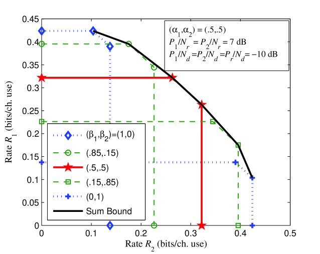
Figure 3: Rate region achieved at the destination for a two-user MARC and $\alpha_{1}=\alpha_{2}=1/2$.

We now consider the special case  in which $\underline{\alpha}_{\mathcal{S}}\not=\underline{1}$ and $\underline{\beta}_{\mathcal{S}^{c}}$ are fixed. We determine a $\underline{\beta}_{\mathcal{S}}$ that maximizes $I_{d,\mathcal{S}}$ subject to (167) and (166). Since $I_{d,\mathcal{S}}$ is a continuous concave function of $\underline{\beta}_{\mathcal{S}}$ it achieves its maximum at a $\beta$${}_{\mathcal{S}}^{\ast}$ where

$$\begin{array}[c]{cc}\left.\frac{\partial I_{d,\mathcal{S}}}{\partial\beta_{k}}\right|_{\beta_{k}^{\ast}}=0&\text{for all }k\in\mathcal{S}\text{.}\end{array}$$ (168)

As before, using Lagrange multipliers, the optimal $\beta$${}_{\mathcal{S}}^{\ast}$ that maximizes $I_{d,\mathcal{S}}$, subject to (167), has entries

$$\beta_{k}^{\ast}=\left\{\begin{array}[c]{cc}\frac{c\left(1-\alpha_{k}\right)P_{k}}{\sum\limits_{k\in\mathcal{S}}\left(1-\alpha_{k}\right)P_{k}}&k\in\mathcal{S}\end{array}\right..$$ (169)

Rate region for a fixed $\alpha$_K: For any choice of a non-zero $\alpha$_K and a $\beta$_K satisfying (165), the rate region given by (164) for all $\mathcal{S}$ is a polymatroid. For $\alpha$${}_{\mathcal{K}}=\underline{1}$, from (164) we see that there are no gains achieved from coherent combining, i.e., it suffices to choose $\beta$${}_{\mathcal{K}}=\underline{0}$. Consider $\alpha$${}_{\mathcal{K}}\not=\underline{1}$. Since there is at least one $k$ for which $\alpha_{k}<1$, gains from coherent combining at the destination are maximized by choosing $\beta$_K to satisfy (165) with equality. For a fixed $\alpha$_K, we then write the rate region at the destination as a union over all polymatroids, one for each choice of $\beta$_K satisfying

$$\sum_{k=1}^{K}\beta_{k}=1.$$ (170)

Observe that for $\underline{\beta}_{\mathcal{K}}^{\ast}$ with entries given by (169), the bound $I_{d,\mathcal{S}}$ is maximized. In Fig 3, we illustrate the rate region for a two-user degraded Gaussian MARC with the SNR$\ P_{1}/N_{d}=P_{2}/N_{d}$ chosen as $-10$ dB, $\alpha$ $=$ $(1/2,1/2)$, and five choices of $\beta$_K. Observe that the maximum single-user rate $R_{1}$ is achieved by setting $\beta_{1}$ to $1$ though this value does not maximize $R_{2}$ or $R_{1}+R_{2}$. For all other $(\beta_{1},\beta_{2})$ such as $(0.85,0.15)$, as $\beta_{1}$ decreases and $\beta_{2}$ increases, $R_{1}$ decreases while $R_{2}$ increases achieving its maximum at $\beta_{2}=1$. The bound on the sum rate $R_{1}+R_{2}$ increases from $(\beta_{1},\beta_{2})=(1,0)$, achieves its maximum at $(\beta_{1}^{\ast},\beta_{2}^{\ast})$ $=$ $(1/2,1/2)$, and then decreases as $\beta_{2}$ approaches $1$. The resulting region at the destination is shown in Fig. 3 as a union over all polymatroids, one for each choice of $\beta$_K.

Appendix D $B_{r,\mathcal{S}}$ vs. $\gamma$_K

We show that the function $B_{r,\mathcal{S}}$ in (10) is a concave function of $\underline{\gamma}_{\mathcal{S}}$ for a fixed $\underline{\gamma}_{\mathcal{S}^{c}}$ and for all $\mathcal{S\subseteq K}$. Recall the expression for $B_{r,\mathcal{S}}$ as

$$B_{r,\mathcal{S}}=C\left({\textstyle\sum\limits_{k\in\mathcal{S}}}\frac{P_{k}}{N_{r}}-\frac{\left(\sum\limits_{k\in\mathcal{S}}\sqrt{\gamma_{k}P_{k}}\right)^{2}}{N_{r}\left(1-{\textstyle\sum\limits_{k\in\mathcal{S}^{c}}}\gamma_{k}\right)}\right)$$ (171)

where we assume that

$$\sum\limits_{k\in\mathcal{S}^{c}}\gamma_{k}=1-c<1.$$ (172)

Observe that $B_{r,\mathcal{S}}$ is maximized when $c=1$, i.e., $\gamma_{k}=0$ for all $k\in\mathcal{S}$, and minimized for $c=0$. Further, comparing $B_{r,\mathcal{S}}$ and $B_{d,\mathcal{S}}$, one can see that for

$$\gamma_{k}=\left\{\begin{array}[c]{lll}P_{k}\left/\left(\sum_{k\in\mathcal{S}}P_{k}\right)\right.&,&k\in\mathcal{S}\\ 0&,&k\in\mathcal{S}^{c}\end{array}\right.$$ (173)

$B_{r,\mathcal{S}}$ achieves its minimum, i.e., $B_{r,\mathcal{S}}=0$.

We write

$$x\overset{\vartriangle}{=}\left(\sum\limits_{k\in\mathcal{S}}\sqrt{\gamma_{k}\lambda_{k}}\right)$$ (174)

where

$$\begin{array}[c]{ccc}P_{\max}=\max_{k\in\mathcal{K}}P_{k}&\text{and}&\lambda_{k}=\left.P_{k}\right/P_{\max}\text{.}\end{array}$$ (175)

Substituting (174) in the expression for $B_{r,\mathcal{S}}$ in (171), we have

$$B_{r,\mathcal{S}}=C\left({\textstyle\sum\limits_{k\in\mathcal{S}}}\frac{P_{k}}{N_{r}}-\frac{x^{2}P_{\max}}{N_{r}c}\right).$$ (176)

Differentiating $B_{r,\mathcal{S}}$ with respect to $x$ we have

$$\frac{dB_{r,\mathcal{S}}}{dx} =\frac{-xP_{\max}}{N_{r}c}\cdot\left(1+{\textstyle\sum\limits_{k\in\mathcal{S}}}\frac{P_{k}}{N_{r}}-\frac{x^{2}P_{\max}}{N_{r}c}\right)^{-1}$$ (177)

$$\frac{d^{2}B_{r,\mathcal{S}}}{dx^{2}} =\frac{-\frac{P_{\max}}{N_{r}c}\left(1+{\textstyle\sum\limits_{k\in\mathcal{S}}}\frac{P_{k}}{N_{r}}\right)-\left(\frac{xP_{\max}}{N_{r}c}\right)^{2}}{\left(1+{\textstyle\sum\limits_{k\in\mathcal{S}}}\frac{P_{k}}{N_{r}}-\frac{x^{2}P_{\max}}{N_{r}c}\right)^{2}}$$ (178)

$$<0$$ (179)

where the strict inequality in (179) follows since all terms in (178) are positive. Further, for any $c>0\,$, from (176) $B_{r,\mathcal{S}}$ is maximized at $x=0$, i.e., for $\gamma_{k}=0$ for all $k\in\mathcal{S}$. Thus, we see that $B_{r,\mathcal{S}}$ is a concave decreasing function of $x$.

Appendix E Proof of Theorem 5

We now prove Theorem 5 and give the solution to the max-min optimization

$$R_{\mathcal{K}}=\max\limits_{\underline{\gamma}_{\mathcal{K}}\in\Gamma_{OB}}\min\left(B_{r,\mathcal{K}}\left(\underline{\gamma}_{\mathcal{K}}\right),B_{d,\mathcal{K}}\left(\underline{\gamma}_{\mathcal{K}}\right)\right).$$ (180)

Consider the function

$$\begin{array}[c]{cc}J(\underline{\gamma}_{\mathcal{K}},\delta)=\delta B_{r,\mathcal{K}}\left(\underline{\gamma}_{\mathcal{K}}\right)+\left(1-\delta\right)B_{d,\mathcal{K}}\left(\underline{\gamma}_{\mathcal{K}}\right),&\delta\in[0,1].\end{array}$$ (181)

Observe that $J$ is linear in $\delta$ ranging in value from $I_{d,\mathcal{K}}$ for $\delta$ $=$ $0$ to $I_{r,\mathcal{K}}$ for $\delta=1$. Thus, the optimization in (181) is equivalent to maximizing the minimum of the two end points of the line $J$ over $\Gamma_{OB}$. Maximizing $J(\underline{\gamma}_{\mathcal{K}},\delta)$ over $\underline{\gamma}_{\mathcal{K}}$, we obtain a continuous convex function

$$\begin{array}[c]{cc}V(\delta)=\max\limits_{\underline{\gamma}_{\mathcal{K}}\in\Gamma_{OB}}J(\underline{\gamma}_{\mathcal{K}},\delta),&\delta\in[0,1].\end{array}$$ (182)

From (181) and (182), we see that for any $\underline{\gamma}_{\mathcal{K}}$, $J(\underline{\gamma}_{\mathcal{K}},\delta)$ either lies strictly below or is tangential to $V(\delta)$. The following proposition summarizes a well-known solution to the max-min problem in (180) (see [9]).

Proposition 3

$\underline{\gamma}_{\mathcal{K},\mathcal{\delta}^{\ast}}^{\ast}$ is a max-min rule where

$$\delta^{\ast}=\arg\min_{\delta\in[0,1]}V(\delta).$$ (183)

The maximum bound on $R_{\mathcal{K}}$, $V(\delta^{\ast})$, is completely determined by the following three cases (see Fig. 4).

$$\begin{array}[c]{cl}\text{Case 1:}&\delta^{\ast}=0:V(\delta^{\ast})=B_{d,\mathcal{K}}(\underline{\gamma}_{\mathcal{K},\mathcal{\delta}^{\ast}}^{\ast})<B_{r,\mathcal{K}}(\underline{\gamma}_{\mathcal{K},\mathcal{\delta}^{\ast}}^{\ast})\end{array}$$ (185)

$$\begin{array}[c]{cl}\text{Case 2:}&\delta^{\ast}=1:V(\delta^{\ast})=B_{r,\mathcal{K}}(\underline{\gamma}_{\mathcal{K},\mathcal{\delta}^{\ast}}^{\ast})<B_{d,\mathcal{K}}(\underline{\gamma}_{\mathcal{K},\mathcal{\delta}^{\ast}}^{\ast})\end{array}$$ (187)

$$\begin{array}[c]{cl}\text{Case 3:}&0<\delta^{\ast}<1:V(\delta^{\ast})=B_{r,\mathcal{K}}(\underline{\gamma}_{\mathcal{K},\mathcal{\delta}^{\ast}}^{\ast})=B_{d,\mathcal{K}}(\underline{\gamma}_{\mathcal{K},\mathcal{\delta}^{\ast}}^{\ast}).\end{array}$$ (189)

We apply Proposition 3 to determine the maximum bound on $R_{\mathcal{K}}$. We study each case separately and determine the max-min rule $\underline{\gamma}_{\mathcal{K}}^{\ast}$ for each case. In general, the max-min rule $\underline{\gamma}_{\mathcal{K},\mathcal{\delta}^{\ast}}^{\ast}$ depends on an optimal $\mathcal{\delta}^{\ast}$. However, for notational convenience we henceforth omit the subscript $\delta^{\ast}$ in denoting the max-min rule. We develop the optimal $\underline{\gamma}_{\mathcal{K}}^{\ast}$ and the maximum sum-rate for each case. We first consider case $1$ and show that this case is not feasible.

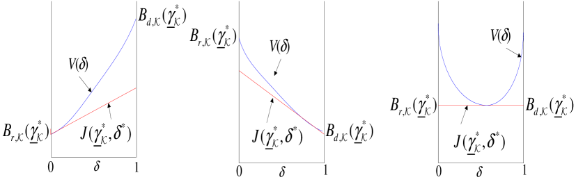
Figure 4: Illustration of Cases 1, 2, and 3.

Case 1: This case occurs when the maximum bound achievable at the destination is smaller than the bound at the relay. In Appendix C, we show that the bound $B_{d,\mathcal{K}}(\underline{\gamma}_{\mathcal{K}})$ is a concave function of $\underline{\gamma}_{\mathcal{K}}$ and achieves a maximum at $\gamma$${}_{\mathcal{K}}^{\ast}$ whose entries $\gamma_{k}^{\ast}$ satisfy (121) and are given as

$$\begin{array}[c]{cc}\gamma_{k}^{\ast}=P_{k}\left/\left(\sum_{k\in\mathcal{K}}P_{k}\right)\right.,&\text{for all }k\in\mathcal{K}\text{.}\end{array}$$ (190)

Substituting (190) in (10), we have $B_{r,\mathcal{K}}(\underline{\gamma}_{\mathcal{K}}^{\ast})=0$ which contradicts the assumption in (185), thus making this case infeasible.

Case 2: Consider the condition for case 2 in (187). This condition implies that the case occurs when the maximum bound achievable at the relay is smaller than the bound at the destination. From (64), we observe that $B_{r,\mathcal{K}}$ decreases monotonically with $\gamma_{k}$ for all $k$ and achieves a maximum of

$$B_{r,\mathcal{K}}(\underline{\gamma}_{\mathcal{K}}^{\ast})=C\left(\frac{{\textstyle\sum\limits_{k\in\mathcal{K}}}P_{k}}{N_{r}}\right)$$ (191)

at $\underline{\gamma}_{\mathcal{K}}^{\ast}=\underline{0}$. Comparing (10) and (11) at $\underline{\gamma}_{\mathcal{K}}^{\ast}$ $=$ $\underline{0}$, we obtain the condition for this case as

$$\frac{{\textstyle\sum\limits_{k\in\mathcal{K}}}P_{k}}{N_{r}}\leq\frac{{\textstyle\sum\limits_{k\in\mathcal{K}}}P_{k}+P_{r}}{N_{d}}\text{.}$$ (192)

Case 3: Finally, consider the condition for Case 3 in (189). This case occurs when the maximum rate bound achievable at the relay and destination are equal. The max-min solution for this case is obtained by considering two sub-cases. The first is the relatively straightforward sub-case where $\underline{\gamma}_{\mathcal{K}}^{\ast}$ $=$ $\underline{0}$ is the max-min rule. The resulting maximum sum-rate is the same as that for case $2$ with the condition in (192) satisfied with equality. Consider the second sub-case where $\underline{\gamma}_{\mathcal{K}}^{\ast}$ $\not=$ $\underline{0}$, i.e., when

$$\frac{{\textstyle\sum\limits_{k\in\mathcal{K}}}P_{k}}{N_{r}}>\frac{{\textstyle\sum\limits_{k\in\mathcal{K}}}P_{k}+P_{r}}{N_{d}}\text{.}$$ (193)

We formulate the optimization problem for this case as

$$\begin{array}[c]{ll}\text{maximize}&B_{r,\mathcal{K}}\left(\underline{\gamma}\right)\\ \text{subject to}&B_{r,\mathcal{K}}\left(\underline{\gamma}\right)=B_{d,\mathcal{K}}\left(\underline{\gamma}\right).\end{array}$$ (194)

We write

$$\begin{array}[c]{cc}P_{\max}=\max_{k\in\mathcal{K}}P_{k},&\lambda_{k}=\left.P_{k}\right/P_{\max}\text{,}\end{array}$$ (195)

and define

$$x\overset{\vartriangle}{=}\sqrt{{\textstyle\sum\limits_{k\in\mathcal{K}}}\lambda_{k}\gamma_{k}}.$$ (196)

Substituting (195) and (196) in (10) and (11), we have

$$B_{r,\mathcal{K}}(x) =C\left(\frac{\left({\textstyle\sum\limits_{k\in\mathcal{K}}}P_{k}\right)-x^{2}P_{\max}}{N_{r}}\right)$$ (197)

$$B_{d,\mathcal{K}}(x) =C\left(\frac{\left({\textstyle\sum\limits_{k\in\mathcal{K}}}P_{k}\right)+P_{r}+2x\sqrt{P_{\max}P_{r}}}{N_{d}}\right).$$ (198)

Observe that $B_{r,\mathcal{K}}(x)$ and $B_{d,\mathcal{K}}(x)$ are monotonically decreasing and increasing functions of $x$, respectively, and thus, the maximization in (194) simplifies to determining an $x$ such that

$$\frac{{\textstyle\sum\limits_{k\in\mathcal{K}}}P_{k}-x^{2}P_{\max}}{N_{r}}=\frac{{\textstyle\sum\limits_{k\in\mathcal{K}}}P_{k}+P_{r}+2x\sqrt{P_{\max}P_{r}}}{N_{d}}.$$ (199)

We write

$$\begin{array}[c]{lll}K_{0}=P_{\max}\left/N_{r}\right.,&&K_{1}=\sqrt{P_{\max}P_{r}}\left/N_{d}\right.\\ K_{2}=\frac{\sum\nolimits_{k\in\mathcal{K}}P_{k}}{N_{d}}+\frac{P_{r}}{N_{d}},&\text{and}&K_{3}=\frac{{\textstyle\sum\nolimits_{k\in\mathcal{K}}}P_{k}}{N_{r}}.\end{array}$$ (200)

From (87), since $K_{3}>K_{2}$, the quadratic equation in (199) has only one positive solution given by

$$x^{\ast}=\frac{-K_{1}+\sqrt{K_{1}^{2}+\left(K_{3}-K_{2}\right)K_{0}}}{K_{0}}.$$ (201)

The optimal power policy for this case is then the set $\mathcal{G}$ of $\underline{\gamma}_{\mathcal{K}}^{\ast}$ for which $\underline{\gamma}_{\mathcal{K}}^{\ast}$ satisfies (196) with $x=$ $x^{\ast}$ in (201). The maximum achievable sum-rate for this case is then obtained from (197) as

$$C\left(\frac{{\textstyle\sum\limits_{k\in\mathcal{K}}}P_{k}-\left(x^{\ast}\right)^{2}P_{\max}}{N_{r}}\right).$$ (202)

Appendix F Proof of Theorem 11

We now prove Theorem 11 and give the solution to the max-min optimization

$$R_{\mathcal{K}}=\max\limits_{(\underline{\alpha}_{\mathcal{K}},\underline{\beta}_{\mathcal{K}})\in\Gamma}\min\left(I_{r,\mathcal{K}}\left(\underline{\alpha}_{\mathcal{K}}\right),I_{d,\mathcal{K}}\left(\underline{\alpha}_{\mathcal{K}},\underline{\beta}_{\mathcal{K}}\right)\right).$$ (203)

As in Appendix E, a solution to the max-min optimization in (203) simplifies to three mutually exclusive cases [16, II.C] such that the max-min rule $(\underline{\alpha}_{\mathcal{K}}^{\ast},\underline{\beta}_{\mathcal{K}}^{\ast})$ satisfies the conditions for one of three cases. The conditions for the three cases are

$$\begin{array}[c]{cc}\text{Case }1\text{:}&I_{d,\mathcal{K}}(\underline{\alpha}_{\mathcal{K}}^{\ast},\underline{\beta}_{\mathcal{K}}^{\ast})<I_{r,\mathcal{K}}(\underline{\alpha}_{\mathcal{K}}^{\ast})\end{array}$$ (205)

$$\begin{array}[c]{cc}\text{Case }2\text{:}&I_{r,\mathcal{K}}(\underline{\alpha}_{\mathcal{K}}^{\ast})<I_{d,\mathcal{K}}(\underline{\alpha}_{\mathcal{K}}^{\ast},\underline{\beta}_{\mathcal{K}}^{\ast})\end{array}$$ (207)

$$\begin{array}[c]{cc}\text{Case }3\text{:}&I_{r,\mathcal{K}}(\underline{\alpha}_{\mathcal{K}}^{\ast})=I_{d,\mathcal{K}}(\underline{\alpha}_{\mathcal{K}}^{\ast},\underline{\beta}_{\mathcal{K}}^{\ast})\end{array}$$ (209)

We develop the conditions and determine the max-min rule for each case. We first consider case $1$ and show that this case is not feasible.

Case 1: This case occurs when the maximum bound achievable at the destination is smaller than the bound at the relay. Observe that $I_{d,\mathcal{K}}(\underline{\alpha}_{\mathcal{K}},\underline{\beta}_{\mathcal{K}})$ in (65) decreases monotonically with $\alpha_{k}$, for all $k$, and, for any $\beta$_K, achieves a maximum at $\alpha$${}_{\mathcal{K}}^{\ast}$ $=$ $0$ of

$$I_{d,\mathcal{K}}(\underline{\alpha}_{\mathcal{K}}^{\ast},\underline{\beta}_{\mathcal{K}})=C\left(\frac{{\textstyle\sum\limits_{k\in\mathcal{K}}}P_{k}+P_{r}+2{\textstyle\sum\limits_{k\in\mathcal{K}}}\sqrt{\beta_{k}P_{k}P_{r}}}{N_{d}}\right).$$ (210)

However, substituting $\alpha$${}_{\mathcal{K}}^{\ast}$ $=$ $0$ in (64), we obtain

$$I_{r,\mathcal{K}}(\underline{\alpha}_{\mathcal{K}}^{\ast})=0$$ (211)

which contradicts the assumption in (205), thus making this case infeasible.

Case 2: Consider the condition for Case 2 in (207). This condition implies that the case occurs when the maximum bound achievable at the relay is smaller than the bound at the destination. From (64), we observe that $I_{r,\mathcal{K}}$ increases monotonically with $\alpha_{k}$ for all $k$ and achieves a maximum of

$$I_{r,\mathcal{K}}(\underline{\alpha}_{\mathcal{K}}^{\ast})=C\left(\frac{{\textstyle\sum\limits_{k\in\mathcal{K}}}P_{k}}{N_{r}}\right)$$ (212)

at $\underline{\alpha}_{\mathcal{K}}^{\ast}=\underline{1}$. Comparing (64) and (65) at $\underline{\alpha}_{\mathcal{K}}^{\ast}$ $=$ $\underline{1}$, we obtain the condition for this case as

$$\frac{{\textstyle\sum\limits_{k\in\mathcal{K}}}P_{k}}{N_{r}}\leq\frac{{\textstyle\sum\limits_{k\in\mathcal{K}}}P_{k}+P_{r}}{N_{d}}\text{.}$$ (213)

Case 3: Finally, consider Case 3 in (209). This case occurs when the maximum rate bound achievable at the relay and destination are equal. The max-min solution for this case is obtained by considering two sub-cases. The first is the relatively straightforward sub-case where $\underline{\alpha}_{\mathcal{K}}^{\ast}$ $=$ $\underline{1}$ is the max-min rule. The resulting maximum sum-rate is the same as that for case $2$ with the condition in (213) satisfied with equality. Consider the second sub-case where $\underline{\alpha}_{\mathcal{K}}^{\ast}$ $\not=$ $\underline{1}$, i.e.,

$$\frac{{\textstyle\sum\limits_{k\in\mathcal{K}}}P_{k}}{N_{r}}>\frac{{\textstyle\sum\limits_{k\in\mathcal{K}}}P_{k}+P_{r}}{N_{d}}\text{.}$$ (214)

In Appendix C we show that, for a fixed $\alpha$_K, $I_{d,\mathcal{S}}$, is a concave function of $\beta$_K for all $\mathcal{S}\subseteq\mathcal{K}$. Furthermore, from (62), for $\alpha$_K $\not=$ $1$, $I_{d,\mathcal{K}}$ in (65) is maximized by a $\underline{\beta}_{\mathcal{K}}^{\ast}$ whose entries $\beta_{k}^{{}^{\ast}}$, for all $k\in\mathcal{K}$, satisfy

$${\textstyle\sum\limits_{k\in\mathcal{K}}}\beta_{k}^{{}^{\ast}}=1$$ (215)

and are given as

$$\begin{array}[c]{cc}\beta_{k}^{\ast}=\left\{\begin{array}[c]{ll}\frac{\left(1-\alpha_{k}\right)P_{k}}{\sum_{k=1}^{K}\left(1-\alpha_{k}\right)P_{k}}&\underline{\alpha}_{\mathcal{K}}\not=\underline{1}\\ 0&\underline{\alpha}_{\mathcal{K}}=\underline{1}\end{array}\right.&\text{for all }k\in\mathcal{K}.\end{array}$$ (216)

Observe that the optimal power fraction $\beta_{k}^{{}^{\ast}}$ that the relay allocates to cooperating with user $k$ is proportional to the power allocated by user $k$ to achieve coherent combining gains at the destination. Thus, one can formulate the optimization problem for this case as

$$\begin{array}[c]{ll}\text{maximize}&I_{r,\mathcal{K}}\left(\underline{\alpha}\right)\\ \text{subject to}&I_{r,\mathcal{K}}\left(\underline{\alpha}\right)=I_{d,\mathcal{K}}\left(\underline{\alpha},\underline{\beta}\right),\\ &{\textstyle\sum\limits_{k\in\mathcal{K}}}\beta_{k}=1.\end{array}$$ (217)

Using Lagrange multipliers we can show that it suffices to consider $\beta_{k}=\beta_{k}^{{}^{\ast}}$ in the maximization. Since the optimal $\beta_{k}^{\ast}$ in (216) is a function of $\alpha$_K, $I_{d,\mathcal{K}}(\underline{\alpha}_{\mathcal{K}},\underline{\beta}_{\mathcal{K}}^{\ast})$ simplifies to a function of $\underline{\alpha}_{\mathcal{K}}$ as

$$I_{d,\mathcal{K}}(\underline{\alpha}_{\mathcal{K}},\underline{\beta}_{\mathcal{K}}^{\ast})=C\left(\frac{{\textstyle\sum\limits_{k\in\mathcal{K}}}P_{k}+P_{r}+2\sqrt{{\textstyle\sum\limits_{k\in\mathcal{K}}}\left(1-\alpha_{k}\right)P_{k}P_{r}}}{N_{d}}\right).$$ (218)

We further simplify $I_{d,\mathcal{K}}(\underline{\alpha}_{\mathcal{K}},\underline{\beta}_{\mathcal{K}}^{\ast})$ and $I_{r,\mathcal{K}}(\underline{\alpha}_{\mathcal{K}})$ as follows. We write

$$\begin{array}[c]{cc}P_{\max}=\max_{k\in\mathcal{K}}P_{k},&\lambda_{k}=\left.P_{k}\right/P_{\max}\text{,}\end{array}$$ (219)

and

$$q\overset{\vartriangle}{=}\sqrt{{\textstyle\sum\limits_{k\in\mathcal{K}}}\left(1-\alpha_{k}\right)\lambda_{k}}.$$ (220)

Substituting (219) and (220) in (64) and (65), we have

$$I_{r,\mathcal{K}}(q) =C\left(\frac{\left({\textstyle\sum\limits_{k\in\mathcal{K}}}P_{k}\right)-q^{2}P_{\max}}{N_{r}}\right)$$ (221)

$$I_{d,\mathcal{K}}(q) =C\left(\frac{\left({\textstyle\sum\limits_{k\in\mathcal{K}}}P_{k}\right)+P_{r}+2q\sqrt{P_{\max}P_{r}}}{N_{d}}\right).$$ (222)

Observe that $I_{r,\mathcal{K}}(q)$ and $I_{d,\mathcal{K}}(q)$ are monotonically increasing and decreasing functions of $q$ and thus, the maximization in (217) simplifies to determining a $q$ such that

$$\frac{{\textstyle\sum\limits_{k\in\mathcal{K}}}P_{k}-q^{2}P_{\max}}{N_{r}}=\frac{{\textstyle\sum\limits_{k\in\mathcal{K}}}P_{k}+P_{r}+2q\sqrt{P_{\max}P_{r}}}{N_{d}}.$$ (223)

The condition in (223) has the geometric interpretation that the bounds on $R_{\mathcal{K}}$ are maximized when the $K$-user sum rate plane achieved at the relay is tangential to the concave sum-rate surface achieved at the destination at its maximum value. We further simplify (223) by using the definitions in Appendix E for $K_{0}$, $K_{1}$, $K_{2}$, and $K_{3}$. From (214), since $K_{3}>K_{2}$, the quadratic equation in (223) has only one positive solution given by

$$q^{\ast}=\frac{-K_{1}+\sqrt{K_{1}^{2}+\left(K_{3}-K_{2}\right)K_{0}}}{K_{0}}.$$ (224)

The optimal power policy for this case is then the set $\mathcal{P}$ of $(\underline{\alpha}_{\mathcal{K}}^{\ast},\underline{\beta}_{\mathcal{K}}^{\ast}(\underline{\alpha}_{\mathcal{K}}^{\ast}))$ such that $\underline{\alpha}_{\mathcal{K}}^{\ast}$ satisfies (220) for $q=$ $q^{\ast}$ and for each such choice of $\underline{\alpha}_{\mathcal{K}}^{\ast}$, $\underline{\beta}_{\mathcal{K}}^{\ast}$ is given by (216). The maximum achievable sum-rate for this case is then given by

$$C\left(\frac{\left({\textstyle\sum\limits_{k\in\mathcal{K}}}P_{k}\right)-\left(q^{\ast}\right)^{2}P_{\max}}{N_{r}}\right).$$ (225)

Remark 12

The optimal $q^{\ast}$ in (224) is the same as the optimal $x^{\ast}$ in (201). Further, the maximum inner (DF) and outer bounds on the sum-rate are also the same for the equal-bounds case in (225) and (202), respectively.

Appendix G Sum-Capacity Proof for the Active Class

In Theorem 12, we proved that DF achieves the sum-capacity for an active class of degraded Gaussian MARCs. In the proof we argue that since the maximum DF sum-rate is the same as the maximum outer bound sum-rate, every DF max-min rule $(\underline{\alpha}_{\mathcal{K}}^{\ast},\underline{\beta}_{\mathcal{K}}^{\ast})\in\mathcal{P}_{a}$ that achieves this maximum sum-rate, i.e., for which $R_{r}(\underline{\alpha}_{\mathcal{K}}^{\ast})\cap R_{d}(\underline{\alpha}_{\mathcal{K}}^{\ast},\underline{\beta}_{\mathcal{K}}^{\ast})$ belongs to the set of active cases, also achieves the sum-capacity. We now present a more detailed proof of the argument.

We begin by comparing the inner and outer bounds. As in the symmetric case, without loss of generality, we write

$$\begin{array}[c]{cc}\gamma_{k}=\left(1-\alpha_{k}\right)\beta_{k}&\text{for all }k\end{array}$$ (226)

where $(\underline{\alpha}_{\mathcal{K}},\underline{\beta}_{\mathcal{K}})\in\Gamma.$ We then have,

$$B_{r,\mathcal{K}}(\underline{\alpha}_{\mathcal{K}},\underline{\beta}_{\mathcal{K}})=C\left({\textstyle\sum\limits_{k\in\mathcal{K}}}\frac{P_{k}}{N_{r}}-\frac{\left(\sum\limits_{k\in\mathcal{K}}\sqrt{\left(1-\alpha_{k}\right)\beta_{k}P_{k}}\right)^{2}}{N_{r}}\right)$$ (227)

and

$$B_{d,\mathcal{K}}(\underline{\alpha}_{\mathcal{K}},\underline{\beta}_{\mathcal{K}})=C\left(\frac{{\textstyle\sum\limits_{k\in\mathcal{K}}}P_{k}+P_{r}+2{\textstyle\sum\limits_{k\in\mathcal{K}}}\sqrt{\left(1-\alpha_{k}\right)\beta_{k}P_{k}P_{r}}}{N_{d}}\right)=I_{d,\mathcal{K}}(\underline{\alpha}_{\mathcal{K}},\underline{\beta}_{\mathcal{K}}).$$ (228)

Choosing $\underline{\beta}_{\mathcal{K}}$ as the DF max-min rule $\underline{\beta}_{\mathcal{K}}^{\ast}$ in (76), simplifies (227) to

$$B_{r,\mathcal{K}}(\underline{\alpha}_{\mathcal{K}},\underline{\beta}_{\mathcal{K}}^{\ast})=C\left({\textstyle\sum\limits_{k\in\mathcal{K}}}\frac{\alpha_{k}P_{k}}{N_{r}}\right)=I_{r,\mathcal{K}}(\underline{\alpha}_{\mathcal{K}}).$$ (229)

Using theorem 11, one can then verify that $B_{r,\mathcal{K}}(\underline{\alpha}_{\mathcal{K}}^{\ast},\underline{\beta}_{\mathcal{K}}^{\ast})=B_{d,\mathcal{K}}(\underline{\alpha}_{\mathcal{K}}^{\ast},\underline{\beta}_{\mathcal{K}}^{\ast})$ is achieved by all $\underline{\alpha}_{\mathcal{K}}^{\ast}\in\mathcal{P}$. Consider a $\underline{\alpha}_{\mathcal{K}}^{\ast}\in\mathcal{P}_{a}$ and a corresponding $\beta_{\mathcal{K}}^{\ast}$ such that the DF region $\mathcal{R}_{r}(\underline{\alpha}_{\mathcal{K}}^{\ast})\cap\mathcal{R}_{d}(\underline{\alpha}_{\mathcal{K}}^{\ast},\underline{\beta}_{\mathcal{K}}^{\ast})$ belongs to the set of active cases. From Theorem 11, this implies that

$$\begin{array}[c]{cc}I_{d,\mathcal{A}}(\underline{\alpha}_{\mathcal{K}}^{\ast},\underline{\beta}_{\mathcal{K}}^{\ast})+I_{r,\mathcal{A}^{c}}(\underline{\alpha}_{\mathcal{K}}^{\ast})>I^{\ast}=B^{\ast}&\text{for all }\mathcal{A}\subset\mathcal{K}.\end{array}$$ (230)

Using (226), we expand $B_{d,\mathcal{S}}$ in (11) as a function of $(\underline{\alpha}_{\mathcal{K}}^{\ast},\underline{\beta}_{\mathcal{K}}^{\ast})$ as

$$B_{d,\mathcal{S}}(\underline{\alpha}_{\mathcal{K}}^{\ast},\underline{\beta}_{\mathcal{K}}^{\ast}) =C\left(\frac{{\textstyle\sum\limits_{k\in\mathcal{K}}}P_{k}+\left(1-\left({\textstyle\sum\limits_{k\in\mathcal{S}^{c}}}\left(1-\alpha_{k}^{\ast}\right)\beta_{k}^{\ast}\right)\right)P_{r}+2{\textstyle\sum\limits_{k\in\mathcal{S}}}\sqrt{\left(1-\alpha_{k}^{\ast}\right)\beta_{k}^{\ast}P_{k}P_{r}}}{N_{d}}\right)$$ (231)

$$\geq I_{d,\mathcal{S}}(\underline{\alpha}_{\mathcal{K}}^{\ast},\underline{\beta}_{\mathcal{K}}^{\ast})$$ (232)

where (232) follows from the fact that $\left(1-\alpha_{k}^{\ast}\right)\beta_{k}^{\ast}\leq\beta_{k}^{\ast}$, for all $k$ and for all $(\underline{\alpha}_{\mathcal{K}}^{\ast},\underline{\beta}_{\mathcal{K}}^{\ast})$. It is, however, not easy to compare $B_{r,\mathcal{S}}(\underline{\alpha}_{\mathcal{K}}^{\ast},\underline{\beta}_{\mathcal{K}}^{\ast})$ with $I_{r,\mathcal{S}}(\underline{\alpha}_{\mathcal{K}}^{\ast})$. Note, however, that the choice of $\gamma_{k}$ in (226) requires the same source-relay correlation values for both the inner and outer bounds. Furthermore, for every choice of Gaussian input distribution with the same $K$ correlation values for both bounds, comparing the degraded cutset and DF bounds in (9) and (54), respectively, for a constant $U$, we have

$$\begin{array}[c]{cc}I(X_{\mathcal{S}};Y_{r}|X_{\mathcal{S}^{c}}X_{r})\geq I(X_{\mathcal{S}};Y_{r}|X_{\mathcal{S}^{c}}V_{\mathcal{K}}X_{r})&\text{for all }\mathcal{S}\subseteq\mathcal{K}\end{array}$$ (233)

where in (233) we use the fact that conditioning does not increase entropy to show that the cutset bounds at the relay are less restrictive than the corresponding DF bounds. From (229), the inequality in (233) simplifies to an equality for $\mathcal{S}=\mathcal{K}$ and for $(\underline{\alpha}_{\mathcal{K}}^{\ast},\underline{\beta}_{\mathcal{K}}^{\ast})\in\mathcal{P}_{a}$ when $\gamma_{k}$ is given by (226). Combining these inequalities with (230), we then have

$$\begin{array}[c]{cc}B_{d,\mathcal{A}}(\underline{\alpha}_{\mathcal{K}}^{\ast},\underline{\beta}_{\mathcal{K}}^{\ast})+B_{r,\mathcal{A}^{c}}(\underline{\alpha}_{\mathcal{K}}^{\ast})>I^{\ast}=B^{\ast}&\text{for all }\mathcal{A}\subset\mathcal{K}.\end{array}$$ (234)

Thus, every DF max-min rule that results in an active case polymatroid intersection, i.e., every $(\underline{\alpha}_{\mathcal{K}}^{\ast},\underline{\beta}_{\mathcal{K}}^{\ast})\in\mathcal{P}_{a}$, also results in an active case for the outer bounds when $\gamma_{k}$ is given by (226).

References

- [1] G. Kramer and A. J. van Wijngaarden, “On the white Gaussian multiple-access relay channel,” in Proc. 2000 IEEE Int. Symp. Inform. Theory, Sorrento, Italy, June 2000, p. 40.
- [2] E. C. van der Meulen, “Three-terminal communication channels,” Adv. Applied Probability, vol. 3, pp. 120–154, 1971.
- [3] T. Cover and A. El Gamal, “Capacity theorems for the relay channel,” IEEE Trans. Inform. Theory, vol. 25, no. 5, pp. 572–584, Sept. 1979.
- [4] G. Kramer, M. Gastpar, and P. Gupta, “Cooperative strategies and capacity theorems for relay networks,” IEEE Trans. Inform. Theory, vol. 51, no. 9, pp. 3027–3063, Sept. 2005.
- [5] L. Sankaranarayanan, G. Kramer, and N. B. Mandayam, “Capacity theorems for the multiple-access relay channel,” in Proc. 42nd Annual Allerton Conf. on Commun., Control, and Computing, Monticello, IL, Sept. 2004, pp. 1782–1791.
- [6] A. Reznik, S. R. Kulkarni, and S. Verdu, “Capacity and optimal resource allocation in the degraded Gaussian relay channel with multiple relays,” IEEE Trans. Inform. Theory, vol. 50, no. 12, pp. 3037–3046, Dec. 2004.
- [7] L.-L. Xie and P. R. Kumar, “An achievable rate for the multiple-level relay channel,” IEEE Trans. Inform. Theory, vol. 51, no. 4, pp. 1348–1358, Apr. 2005.
- [8] A. El Gamal and M. Aref, “The capacity of the semideterministic relay channel,” IEEE Trans. Inform. Theory, vol. 28, no. 3, p. 536, May 1982.
- [9] Y. Liang, V. Veeravalli, and H. V. Poor, “Resource allocation for wireless fading relay channels: max-min solution,” IEEE Trans. Inform. Theory, vol. 53, no. 10, pp. 3432–3453, Oct. 2007.
- [10] A. El Gamal and S. Zahedi, “Capacity of relay channels with orthogonal components,” IEEE Trans. Inform. Theory, vol. 51, no. 5, pp. 1815–1817, May 2005.
- [11] A. El Gamal and N. Hassanpour, “Capacity theorems for the relay-without-delay channels,” in Proc. 43nd Annual Allerton Conf. on Commun., Control, and Computing, Monticello, IL, Sept. 2005.
- [12] E. C. van der Meulen and P. Vanroose, “The capacity of a relay channel both with and without delay,” IEEE Trans. Inform. Theory, vol. 53, no. 10, pp. 3774–3776, Oct. 2007.
- [13] T. M. Cover and J. A. Thomas, Elements of Information Theory. New York: Wiley, 1991.
- [14] L. Sankaranarayanan, G. Kramer, and N. B. Mandayam, “Hierarchical sensor networks: Capacity theorems and cooperative strategies using the multiple-access relay channel model,” in Proc. First IEEE Conference on Sensor and Ad Hoc Communications and Networks, Santa Clara, CA, Oct. 2004.
- [15] A. Schrijver, Combinatorial Optimization: Polyhedra and Efficiency. New York: Springer-Verlag, 2003.
- [16] H. V. Poor, An Introduction to Signal Detection and Estimation, 2nd. Ed. New York: Springer-Verlag, 1994.
- [17] R. G. Gallager, Information Theory and Reliable Communication. New York: John Wiley, 1968.
- [18] H. G. Eggleston, Convexity. Cambridge, UK: Cambridge University Press, 1958.
- [19] L. Sankar, G. Kramer, and N. B. Mandayam, “Offset encoding for multiaccess relay channels,” IEEE Trans. Inform. Theory, vol. 53, no. 10, pp. 1–8, Oct. 2007.
- [20] J. A. Thomas, “Feedback can at most double Gaussian multiple access channel capacity,” IEEE Trans. Inform. Theory, vol. 33, no. 5, pp. 711–716, Sept. 1987.
- [21] S. Boyd and L. Vandenberghe, Convex Optimization. Cambridge, UK: Cambridge University Press, 2004.