Explicit demonstration of nonabelian anyon, braiding matrix and fusion rules in the Kitaev-type spin honeycomb lattice models

Abstract

The exact solubility of the Kitaev-type spin honeycomb lattice model was proved by means of a Majorana fermion representation or a Jordan-Wigner transformation while the explicit form of the anyon in terms of Pauli matrices became not transparent. The nonabelian statistics of anyons and the fusion rules can only be expressed in indirect ways to Pauli matrices. We convert the ground state and anyonic excitations back to the forms of Pauli matrices and explicitly demonstrate the nonabelian anyonic statistics as well as the fusion rules. These results may instruct the experimental realization of the nonabelian anyons. We suggest a proof-in-principle experiment to verify the existence of the nonabelian anyons in nature.

Introduction The Kitaev-type spin honeycomb lattice models have attracted many research interests for the possible nonabelian anyonic excitations in these exactly soluble two-dimensional models kitaev . There are two topological phases for these kinds of models. The topologically trivial A phase is an abelian anyon phase which is equivalent to that in Kitaev’s toric code model kitaev1 . The topologically nontrivial B phase is within the same universality class of the Moore-Read Pfaffian states in the fractional quantum Hall state mr ; yu and the vortex excitations are nonabelian anyons ms ; w ; mr .

In solving these kinds of models, a key technique is the usage of the Majorana fermion representation of the spin-1/2 operators, either via Kitaev’s Majorana fermions or the Jordan-Winger transformation fzx ; ch ; cn . However, the shortcoming to introduce these Majorana fermions is that the ground state and the elementary excitations are hard to be expressed by the original spin operators, i. e., Pauli matrices. Then the nonabelian fusion rules and statistics may not be directly shown in Pauli matrices’ language ville . Meanwhile, experimentally exciting, manipulating and detecting anyons may be more practical by using the spin operators, as recently suggested or done for the toric code model han ; pan ; pachos ; zoller ; du ; cirac ; bloch and for the A phase of Kitaev honeycomb model zd ; vidal . Therefore, to explicitly demonstrate the nonabelian anyonic statistics, one needs to express the ground state and elementary excitations in the spin operators. Chen and Nussinov cn have studied a real space form of the ground state of the Kitaev honeycomb model and applied it to the A phase with abelian anyons. However, for the more interesting B phase, it was not figured out yet.

In a recent work, one of us, with Wang, has provided a generalized model of the Kitaev honeycomb model by adding three- and four-spin couplings yu ; yu1 . With this generalized Kitaev-type model, we showed the equivalence between the B phase with the breaking of the time reversal symmetry and the Moore-Read Pfaffian state. In that work, we map the model in the honeycomb lattice to a spinless fermion model in a square lattice. The task of the present paper is mapping back the ground state and anyonic(vortex) excitations obtained in the square lattice to their honeycomb lattice version.

After writing down these states in spin operators, i.e., Pauli matrices, we can check the nonabelian statistics of anyons and fusion rules of the excitations. As expected, these results agree with those in the previous abstractive study in Kitaev’s original work kitaev . Moreover, these explicit forms with well-known Pauli matrices may help the readers who are not in this special field to understand those formal descriptions made by Kitaev. It may also instruct the experimentalists to realize these states and verify the existence of the nonabelian anyons in nature. Similar to the case of the abelian anyons in the toric code model zoller ; cirac ; bloch , we may also expect to excite, manipulate and detect the nonabelian anyons in atomic spin systems in optical lattice. We may design a proof-in-principle experiment to show the existence of nonabelian anyon in nature by means of the techniques proposed and developed recently in the photon graph state han ; pan ; pachos , and a nuclear magnetic resonance system du . The minimal lattice needs only six sites, which is accessible to the current experiments, as several experimental groups have done to the toric code model pan ; pachos ; du .

Model and ground state We consider a Kitaev-type spin model in a honeycomb lattice with a three- and four-spin couplings yu ; yu1

$$H = -J_{x}\sum_{x-links}\sigma_{i}^{x}\sigma_{j}^{x}-J_{y}\sum_{y-links}\sigma_{i}^{y}\sigma_{j}^{y}-J_{z}\sum_{z-links}\sigma_{i}^{z}\sigma_{j}^{z}$$ (1)

$$- \kappa\sum_{b}\sigma^{z}_{b}\sigma^{y}_{b+e_{z}}\sigma^{x}_{b+e_{z}+e_{x}}-\kappa\sum_{w}\sigma^{x}_{w}\sigma^{y}_{w+e_{x}}\sigma^{z}_{w+e_{x}+e_{z}}$$

$$- \lambda_{x}\sum_{b}\sigma_{b}^{z}\sigma^{y}_{b+e_{z}}\sigma_{b+e_{z}+e_{x}}^{y}\sigma^{z}_{b+e_{z}+e_{x}+e_{z}}$$

$$- \lambda_{y}\sum_{b}\sigma_{b}^{z}\sigma^{x}_{b+e_{z}}\sigma_{b+e_{z}+e_{y}}^{x}\sigma^{z}_{b+e_{z}+e_{y}+e_{z}},$$

where $\sigma^{x,y,z}$ are Pauli matrices, $x$-,$y$-,$z$-links are shown in Fig. 1, ${}^{\prime}w^{\prime}$ and ${}^{\prime}b^{\prime}$ label the white and black sites of lattice, and $e_{x},e_{y},e_{z}$ are the positive unit vectors, which are defined as, e.g., $e_{a_{1}a_{2}}=e_{z},e_{a_{2}a_{3}}=e_{x},e_{a_{6}a_{1}}=e_{y}$. $J_{x,y,z}$, $\kappa$ and $\lambda_{x,y}$ are tunable real parameters. This is a system with the breaking of the time-reversal symmetry. There is a $Z_{2}$ gauge symmetry generated by

$$W_{P_{a}}=\sigma_{a_{1}}^{x}\sigma_{a_{2}}^{y}\sigma_{a_{3}}^{z}\sigma_{a_{4}}^{x}\sigma_{a_{5}}^{y}\sigma^{z}_{a_{6}}$$ (2)

where $P_{a}$ labels a plaquette (see Fig. 1). That is, $[H,W_{P_{a}}]=0$.

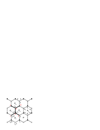
Figure 1: The honeycomb lattice and plaquette. The thick links define $A_{j}$ and also the proof-in-principle configurations.

We first recall how to work out the ground state of this model. The first step is introducing the Majorana fermion representation of the spin operators $\sigma^{a}$ kitaev or employing the Jordan-Wigner transformation fzx ; ch ; cn . For convenience, we use the Jordan-Wigner transformation

$$\psi_{i_{w}}=\sigma_{i_{w}}^{y}\prod_{i^{\prime}_{s}<i_{w}}\sigma^{z}_{i^{\prime}_{s}},~{}~{}\psi_{i_{b}}=\sigma_{i_{b}}^{x}\prod_{i^{\prime}_{s}<i_{b}}\sigma^{z}_{i^{\prime}_{s}},$$

$$b_{i_{w}}=-\sigma_{i_{w}}^{x}\prod_{i^{\prime}_{s}<i_{w}}\sigma^{z}_{i^{\prime}_{s}},~{}~{}b_{i_{b}}=-\sigma_{i_{b}}^{y}\prod_{i^{\prime}_{s}<i_{b}}\sigma^{z}_{i^{\prime}_{s}}$$ (3)

where $i$ lables a $z$-link and $\psi_{i_{s}}$ and $b_{i_{s}}$ are Majorana fermions which satisfy $\psi_{i_{s}}\psi_{j_{t}}=-\psi_{j_{t}}\psi_{i_{s}}$, $b_{i_{s}}b_{j_{t}}=-b_{j_{t}}b_{i_{s}}$ for $i_{s}\neq j_{t}$; and $\psi_{i_{s}}^{2}=b_{j_{t}}^{2}=1$. $\psi_{i_{s}}$ and $b_{j_{t}}$ are also anticommutative. The order of the sites is defined as follows: $i_{s}>j_{t}$ if the zig-zag horizontal line that $i_{s}$ belongs to is higher than that of $j_{t}$ or if $i_{s}$ is on the right hand of $j_{t}$ when they are in the same line.

After this Jordan-Wigner transformation, the Hamiltonian reads

$$H = -iJ_{x}\sum_{x-links}\psi_{w}\psi_{b}-iJ_{y}\sum_{y-links}\psi_{b}\psi_{w}$$

$$- J_{z}\sum_{z-links}b_{w}b_{b}\psi_{b}\psi_{w}-\kappa\sum_{b}b_{b}b_{b+e_{z}}\psi_{b}\psi_{b+e_{z}+e_{x}}$$

$$- \kappa\sum_{w}b_{w+e_{x}}b_{w+e_{x}+e_{z}}\psi_{w}\psi_{w+e_{x}+e_{z}}$$

$$- i\lambda_{y}\sum_{b}b_{b}b_{b+e_{z}}b_{b+e_{z}+e_{y}}b_{b+e_{z}+e_{y}+e_{z}}\psi_{b}\psi_{b+e_{z}+e_{y}+e_{z}}$$

$$- i\lambda_{x}\sum_{b}b_{b}b_{b+e_{z}}b_{b+e_{z}+e_{x}}b_{b+e_{z}+e_{x}+e_{z}}\psi_{b}\psi_{b+e_{z}+e_{x}+e_{z}}.$$

According to Lieb’s theorem lieb , the ground state of the system is $Z_{2}$ vortex free state. This means that $ib_{b}b_{b+e_{z}}=1$ in the ground state sector. Following the track in refs. cn ; yu , finally, the Hamiltonian in the ground state sector is given by

$$H_{0}=J_{z}\sum_{i}(d_{i}^{\dagger}d_{i}-1/2)+i\kappa\sum_{i}(d_{i}d_{i+e_{x}}+d_{i}^{\dagger}d_{i+e_{x}}^{\dagger})$$

$$+\tilde{J}_{x}(d^{\dagger}_{i}d_{i+e_{x}}-d_{i}d_{i+e_{x}}^{\dagger})+\tilde{J}_{y}(d^{\dagger}_{i}d_{i+e_{y}}-d_{i}d_{i+e_{y}}^{\dagger})$$ (5)

$$+\lambda_{x}\sum_{i}(d^{\dagger}_{i+e_{x}}d^{\dagger}_{i}-d_{i+e_{x}}d_{i})+\tilde{\lambda}_{y}\sum_{i}(d^{\dagger}_{i+e_{y}}d^{\dagger}_{i}-d_{i+e_{y}}d_{i})$$

where $\tilde{J}_{x,y}=\frac{J_{x,y}-\lambda_{x,y}}{2}$ and $\tilde{\lambda}_{x,y}=\frac{J_{x,y}+\lambda_{x,y}}{2}$. The spinless fermion $d_{i}=\frac{1}{2}(\psi_{i_{w}}+i\psi_{i_{b}})$ is located at the $z$-link and all $z$-links form a square lattice. Taking $\lambda_{x}+J_{x}=0$ and $\tilde{\lambda}_{y}=\kappa$, this Hamiltonian describes a $p_{x}+ip_{y}$-wave pairing state in this square lattice. As we have shown, the phase diagram consists of two phases: the topologically trial A phase and non-trivial B phase. The phase boundary is the lines:$J_{z}\pm\tilde{J}_{x}\mp\tilde{J}_{y}$ if we restrict to $J_{z}>0$ and $\tilde{J}_{x,y}>0$. The A phase is an abelian anyon phase which is equivalent to that in the toric code model, which was studied before kitaev ; cn . If we do not consider the high energy Majorana fermion excitation, the effective Hamiltonian of the A phase in the honeycomb lattice reads kitaev

$$H_{eff}=-J_{eff}(\sum_{P}W_{P}+\sum_{z-links}A_{j}),$$ (6)

where $A_{j}=\psi_{1}\psi_{3}\psi_{6}\psi_{4}$ (see Fig. 1) with $\lambda_{x,y}=\kappa=0$ and $J_{eff}=\frac{J_{x}^{2}J_{y}^{2}}{16J_{z}^{3}}$ for $J_{x,y}\ll J_{z}$. One may directly check that the ground state is given by

$$|G_{A}\rangle\propto\prod_{j}(1+A_{j})\prod_{P}(1+W_{P})|\phi\rangle,$$ (7)

because $W_{P}|G_{A}\rangle=A_{j}|G_{A}\rangle=|G_{A}\rangle$ with $|\phi\rangle=|\uparrow\cdots\uparrow\rangle$ a reference state. Here the Majorana fermion excitations have a high energy $2J_{z}$ and has been neglected. This Hamiltonian has a $Z_{2}\times Z_{2}$ gauge symmetry generated by $W_{P}$ and $A_{j}$ with $A_{j}^{2}=W_{P}^{2}=1$ and $[A_{j},W_{P}]=0$. We know that $A_{j}$ and $W_{P}$ are corresponding to the ’electric charge’ and ’magnetic charge’ in the toric code model. The low energy excitations have $A_{j}=-1$ or $W_{P}=-1$, which are $e$ and $m$ vortices in the toric code model and obey the mutual semion statistics kitaev . It was noted that the fermion excitations may not be ignored in some braiding processes vidal and there is a controversy to this matter recently con .

In the B phase, we do not have a conserved ’electric charge’ $A_{j}$. Since the ground state sector in the continuous limit is a $p_{x}+ip_{y}$-wave BCS theory, the ground state in the square lattice may be written down, which is yu

$$|G_{B}\rangle=(\sum_{i\neq i^{\prime}}\frac{1}{z_{j}-z_{j^{\prime}}}d^{\dagger}_{j}d^{\dagger}_{j^{\prime}})^{N/2}={\rm Pf}(\frac{1}{z_{j}-z_{j^{\prime}}})\prod_{l}d^{\dagger}_{l}|0\rangle$$ (8)

where $z_{j}=j_{x}+ij_{y}$ is a complex number with $j=(j_{x},j_{y})$ the lattice site label. The vacuum state $|0\rangle$ is defined by $d_{j}|0\rangle=0$ while the state $|D\rangle=\prod_{i}d^{\dagger}_{i}|0\rangle$ satisfies $d^{\dagger}_{j}|D\rangle=0$ because the square lattice is filled. The vacuum state has been written back in terms of Pauli matrices cn , which is given by $|0\rangle\propto\prod_{j}(1-Q_{j})\prod_{P}(1+W_{P})|\phi\rangle$ due to $d_{j}(1-Q_{j})=0$ where $Q_{j}=i\psi_{j_{w}}\psi_{j_{b}}$. $1+W_{P}$ factor is introduced because $W_{P}(1+W_{P})=1+W_{P}$ ensures the vortex free of the ground state, i.e., $W_{P}|G_{B}\rangle=|G_{B}\rangle$. Because of $d_{j}^{\dagger}(1+Q_{j})=0$, $d^{\dagger}_{j}|D\rangle=0$, which is equivalent to $Q_{j}|D\rangle=|D\rangle$. Therefore,

$$|D\rangle\propto\prod_{j}(1+Q_{j})\prod_{P}(1+W_{P})|\phi\rangle.$$ (9)

Excitations A Majorana fermion excitation on the ground state is given by $\psi_{j_{s}}|G_{A,B}\rangle$. Due to $[W_{P},\psi_{j_{s}}]=0$, $\psi_{j_{s}}|G_{A,B}\rangle$ is also a vortex free state. According to the original Hamiltonian, the energy cost to excite a Majorana fermion is given by

$$E_{\psi}-E_{g}=\langle G_{A,B}|\psi_{j_{s}}|H|\psi_{j_{s}}|G_{A,B}\rangle-E_{g}=2J_{z},$$ (10)

where $E_{g}$ is the ground state energy. Note that $\psi_{i_{b}}$ relates to $\psi_{i_{w}}$ by $\psi_{i_{b}}|G_{B}\rangle=-i\psi_{i_{w}}|G_{B}\rangle$.

We are now going to create the vortex excitations which are defined by $W_{P}\sigma_{P}|G_{A,B}\rangle=-\sigma_{P}|G_{A,B}\rangle$ and $W_{P^{\prime}}\sigma_{P}|G_{A,B}\rangle=\sigma_{P}|G_{A,B}\rangle$ for $P^{\prime}\neq P$. Two operators obey these requirements:

$$\sigma^{(1)}_{P}=\sigma_{i_{b}}^{z}\sigma^{z}_{i_{b}-2}\sigma^{z}_{i_{b}-4}\cdots,~{}~{}\sigma^{(2)}_{P}=\sigma^{y}_{i_{b}}\sigma^{z}_{i_{b}-1}\sigma^{z}_{i_{b}-3}\cdots.$$ (11)

The vortex is located at the plaquette $P$ with $i_{b}$ being its ’$a_{1}$’ (See Fig. 1). The sites $i_{b}-1,i_{b}-2,\cdots$ are also marked in Fig. 1. One may also define a vortex at the same plaquette through $\tilde{\sigma}^{(1)}_{P}=\sigma^{z}_{i_{w}}\sigma^{z}_{i_{w}-2}\sigma^{z}_{i_{w}-4}\cdots$ and $\tilde{\sigma}^{(2)}_{P}=\sigma^{x}_{i_{w}}\sigma^{z}_{i_{w}-1}\sigma^{z}_{i_{w}-3}\cdots$.

Creating a single vortex costs an infinite energy, e.g., in the B phase

$$\langle G_{B}|\sigma^{(1)}_{P}|H|\sigma^{(1)}_{P}|G_{B}\rangle=E_{g}+2(J_{x}+J_{y})(i_{b}-(-\infty)).$$ (12)

Therefore, it is impossible to excite a single vortex. However, exciting a pair of vortices spends finite energy which is dependent on the difference of the site labels of two vortices, e.g., two adjacent vortices $(\sigma_{i_{b}}^{z}\sigma^{z}_{i_{b}-2}\sigma^{z}_{i_{b}-4}\cdots)\cdot(\sigma_{i_{b}+2}^{z}\sigma^{z}_{i_{b}}\sigma^{z}_{i_{b}-2}\cdots)=\sigma_{i_{b}+2}^{z}$, which costs energy $4(J_{x}+J_{y})$. In the A phase, the energy cost of a pair of $\sigma^{(1)}$ is $2J_{eff}$, which is much lower than the energy cost to excite $\psi$ as $J_{z}\gg J_{x,y}$. Exciting pairs $\sigma^{(1)}_{P}\sigma^{(2)}_{P^{\prime}}$ and $\sigma^{(2)}_{P}\sigma^{(2)}_{P^{\prime}}$ costs energy $2(2J_{eff}+J_{z})$ and $4(J_{eff}+J_{z})$, which are also the high energy excitations.

Fusion rules To see nonabelain anyonic fusion rules, we focus on the B phase to study the fusion rules. Since $\psi_{i_{s}}^{2}=1$, the fusion rule of the Majorana fermions is $\psi\times\psi=1$. For the vortex excitations, one has

$$\sigma_{P}^{(1)}\cdot\sigma_{P}^{(1)}=1,~{}~{}\sigma_{P}^{(2)}\cdot\sigma_{P}^{(2)}=1,~{}~{}\sigma_{P}^{(1)}\cdot\sigma_{P}^{(2)}\propto\psi_{i_{b}},$$

$$\psi_{i_{b}}\cdot\sigma_{P}^{(1)}\propto\sigma_{P}^{(2)},~{}\psi_{i_{b}}\cdot\sigma_{P}^{(2)}\propto\sigma_{P}^{(1)}.$$ (13)

Define two vortex operators $\sigma_{P}=\alpha\sigma^{(1)}_{P}+\beta\sigma^{(2)}_{P}$ and $\sigma^{\dagger}_{P}=\alpha^{*}\sigma^{(1)}_{P}+\beta^{*}\sigma^{(2)}_{P}$, which obey $\sigma_{P}\sigma^{\dagger}_{P}=|\alpha|^{2}+|\beta|^{2}+i(\alpha\beta^{*}-\alpha^{*}\beta)\psi_{i_{b}}$. We can not distinguish vortex pairs $\sigma_{P}\sigma_{P^{\prime}}$, $\sigma^{\dagger}_{P}\sigma^{\dagger}_{P^{\prime}}$, $\sigma_{P}\sigma^{\dagger}_{P^{\prime}}$ and $\sigma^{\dagger}_{P}\sigma_{P^{\prime}}$ because they are energetically degenerate. This means the equivalence between $\sigma_{P}$ and $\sigma^{\dagger}_{P}$ and the fusion rule for the vortices is $\sigma\times\sigma=1+\psi$. On the other hand, the paired vortices are described by a Pfaffian wave function mr ; yu

$${\rm Pf}\biggl{[}\frac{(z_{j}-z_{i_{P}})(z_{j^{\prime}}-z_{i_{P^{\prime}}})+(j\leftrightarrow j^{\prime})}{z_{j}-z_{j^{\prime}}}\biggr{]},$$ (14)

no matter what kind two vortices are. This also implies the equivalence between $\sigma_{P}$ and $\sigma^{\dagger}_{P}$. Summarily, the fusion rules in the B phase are

$$\psi\times\psi=1,~{}~{}\sigma\times\sigma=1+\psi,~{}~{}\psi\times\sigma=\sigma.$$ (15)

These nonabelian fusion rules are the same as those in the Ising model. All fusions cost energy in the same order as that to create a $\psi$ and a pair of vortices.

Braiding matrix The Majorana fermions are anti-commutative which gives $R^{\psi\psi}_{1}=-1$. To see the braiding matrix elements for the vortices, we rotate vortices counterclockwise. In the B phase, we consider two vortices at $P_{2}$ and $P_{3}$ in Fig. 1. We have two ways to rotate them. One way is moving the vortex at $P_{2}$ to $P_{1}$ first, then moving the vortex at $P_{3}$ to $P_{2}$, and moving that at $P_{1}$ to $P_{3}$ (See Fig. 2(up panel)). This exchanges two vortices and the three steps is given by acting $\sigma^{y}_{j_{b}}\cdot\sigma^{z}_{j_{b}}\cdot\sigma^{x}_{j_{b}}$ in turn on $\sigma_{P_{2}}\sigma_{P_{3}}|G_{B}\rangle$. A single $\sigma^{x,y}$ action means, while one vortex is moving, (say $\sigma_{P_{2}}\to\sigma_{P_{1}}$) another one, say $\sigma_{P_{3}}$, becomes $\sigma^{\prime}_{P_{3}}=\psi\times\sigma_{P_{3}}$. Thus, this exchange is accompanied by non-trivial fusions or creation and annihilation of the Majorana fermions and then the braiding matrix element is denoted by $R^{\sigma\sigma}_{\psi}=\sigma^{y}_{j_{b}}\sigma^{z}_{j_{b}}\sigma^{x}_{j_{b}}=i$. Rotating vortices clockwise, we have ${R^{\sigma\sigma}_{\psi}}^{-1}=\sigma^{x}_{j_{b}}\sigma^{z}_{j_{b}}\sigma^{y}_{j_{b}}=-i$. This also means $R^{\sigma\psi}_{\sigma}=R^{\psi\sigma}_{\sigma}=-i$. Another way to exchange two vortices are moving the vortex at $P_{2}$ to $P_{1}$ and that at $P_{3}$ to $P_{4}$ simultaneously, then moving that at $P_{1}$ to $P_{3}$ and $P_{4}$ to $P_{1}$ in the same time (See Fig. 2(low panel)). This exchange corresponds to $\sigma^{x}_{j_{w}}\sigma^{y}_{j_{b}}\sigma^{x}_{j_{b}}\sigma^{y}_{j_{w}}\sigma_{P_{2}}\sigma_{P_{3}}|G_{B}\rangle=\sigma^{z}_{j_{w}}\sigma^{z}_{j_{b}}\sigma_{P_{2}}\sigma_{P_{3}}|G_{B}\rangle=\sigma_{P_{2}}\sigma_{P_{3}}|G_{B}\rangle$ since $\sigma^{z}_{j_{b}}\sigma^{z}_{j_{w}}|G_{B}\rangle=|G_{B}\rangle$. Simultaneous $\sigma^{y}_{j_{w}}$ and $\sigma^{x}_{j_{b}}$ action creates two Majorana fermions $\psi_{j_{b}}$ and $\psi_{j_{w}}$ but the relation $i\psi_{j_{w}}\psi_{j_{b}}|G_{B}\rangle=|G_{B}\rangle$ means no fermion is created at any stage vidal . This defines a braiding matrix element $R^{\sigma\sigma}_{1}=1$ to exchange. Therefore, the nonabelian braiding matrix for the B phase is given by

$$R^{\psi\psi}_{1}=-1,~{}R^{\sigma\sigma}_{1}=1,~{}R^{\sigma\psi}_{\sigma}=R^{\psi\sigma}_{\sigma}=-i,~{}R^{\sigma\sigma}_{\psi}=i.~{}~{}$$ (16)

Here we do not put in the abelian phase factor $e^{-i\pi/8}$ which comes from the Pfaffian (14). Restoring this phase factor, one has $R^{\sigma\sigma}_{1}=e^{-i\pi/8}$ and $R^{\sigma\sigma}_{\psi}=e^{i3\pi/8}$ and the braid matrix are the same as that of the Ising model ms ; w ; kitaev .

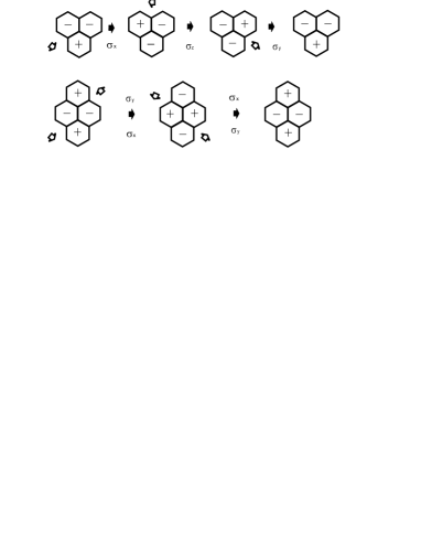
Figure 2: Exchange of the vortices. ’$-$’ at a plaquette labels a vortex. Pauli matrix above the filled arrow means the hermitian rotation operator acting on the white site ’5’ while below the filled arrow means the operator acting on the black site ’2’. Up panel: The exchange leads to a phase factor $i$ for the B phase. Low panel: a bosonic exchange for the B phase. In the A phase, the up panel is forbidden .

Experimental implications Recently, there are several proposals to excite, operate and observe the abelian anyons in the toric code model. Most of them are based on the atoms or molecules in optical lattice zoller ; cirac ; bloch ; zd ; vidal . Since the nonabelian braiding matrix (16) is not related to the Pfaffian factors in eqs. (8) and (14), all the states involved in do not have the site-dependent coefficients if we neglect the Pfaffians. Thus, all techniques applied to the toric code model may be employed to the present model. For example, load cold atoms in a honeycomb optical lattice and manipulate an ancillary atom as proposed in Ref.cirac .

We can also design a possible proof-in-principle experiment to the nonabelian anyons by using the systems to prove the abelian anyons in the toric code model han ; pan ; pachos ; du . As Han et al designed a scheme to demonstrate the abelian anyons in the toric code model, the minimal lattice needed to rotate or exchange two vortices are six sites connected, e.g., by the the thick links in Fig. 1. For this minimal lattice, we prepare the state $|D\rangle$

$$|D\rangle\propto(1+\sigma^{y}_{2}\sigma^{z}_{3}\sigma^{z}_{4}\sigma^{y}_{5})(1+\sigma^{z}_{1}\sigma^{y}_{2}\sigma^{z}_{4}\sigma^{x}_{5})(1+\sigma^{x}_{2}\sigma^{y}_{5}\sigma^{z}_{6}\sigma^{z}_{3})$$

$$(1+\sigma_{1}^{y}\sigma^{x}_{3})(1+\sigma_{4}^{x}\sigma^{y}_{6})|\phi\rangle.$$ (17)

This is an entangled state of 28 pure states and a bit complicated to be prepared experimentally but is still accessible. The two vortices state may be given by, e.g., $\sigma_{2}^{z}|D\rangle$ which creates two vortices at $P_{2}$ and $P_{3}$ because $\{\sigma^{z}_{2},\sigma^{z}_{1}\sigma^{y}_{2}\sigma^{z}_{4}\sigma^{x}_{5}\}=\{\sigma^{z}_{2},\sigma^{x}_{2}\sigma^{y}_{5}\sigma^{z}_{6}\sigma^{z}_{3}\}=0$ and $[\sigma^{z}_{2},\sigma^{y}_{1}\sigma^{z}_{2}\sigma^{x}_{3}]=0$. Two exchanges described before, $\sigma^{x}_{5}\sigma^{y}_{2}\sigma^{x}_{2}\sigma^{y}_{5}$ and $\sigma^{y}_{2}\sigma^{z}_{2}\sigma^{x}_{2}$, result in the signs $\pm$, respectively. A full nonabelian two vortices includes a Pfaffian factor (14), which contributes an abelian phase factor. We do not know if it is possible or not to prepare such a state. Fortunately, to see the nonabelian braiding matrix (16), one needs to simply act a two vortex operator on $|D\rangle$ and check those two different exchanges are enough.

Conclusions We have converted the ground state and elementary excitations from the fermionic representation in a square lattice to the original spin representation in the honeycomb lattice for the Kitaev-type model. Pauli matrix version of these states leads to an explicit demonstration to the non-abelian statistics of anyons in this model. We showed the nonabelain fusion rules and calculated the non-abelian braiding matrices. We proposed a proof-in-principle experiment to create, manipulate and detect the nonabelain anyons in nature.

The authors thank Ville Lahtinen and Julien Vidal for the helpful comments. This work was supported in part by the national natural science foundation of China, the national program for basic research of MOST of China and a fund from CAS.

References

(1)
(2) A. Kitaev, Ann. Phys. 321, 2(2006).
(3) A. Kitaev, Ann. Phys. 303, 2(2003).
(4) G. Moore and N. Read, Nucl. Phys. B 360, 362 (1991).
(5) Yue Yu and Ziqiang Wang, arXiv:0708.0631.
(6) G. Moore and N. Seiberg, Commun. Math.
Phys. 123, 17 (1989).
(7) E. Witten, Commun. Math. Phys. 121, 351 (1989).
(8) X. Y. Feng, G. M. Zhang, and T. Xiang, Phys. Rev. Lett. 98, 087204 (2007).
(9) H. D. Chen and J. P. Hu, Phys. Rev. B 76, 193101 (2007).
(10) H. D. Chen and Z. Nussinov, J. Phys. A 41, 075001
(2008).
(11) Lahtinen et al have derived the nonabelian fusions through the
spectrum analysis (see V. Lahtinen, G. Kells, A. Carollo, T.
Stitt, J. Vala and J. K. Pachos, to appear in Ann. Phys.,
arXiv:0712.1164). However, they are still not directly related to
Pauli matrices.
(12) Y.-J. Han, R. Raussendorf and L.-M. Duan, Phys. Rev.
Lett. 98, 150404 (2007).
(13) C. -Y. Lu, W. -B. Gao,
Otfried Gühne, X. -Q. Zhou, Z. -B. Chen, and J. -W. Pan,
arXiv:0710.0278.
(14)J. K. Pachos, W. Wieczorek, C. Schmid,
N. Kiesel, R. Pohlner, and H. Weinfurter, arXiv:0710.0895.
(15) Liang Jiang, G. K. Brennen, A. V. Gorshkov,
K. Hammerer, M. Hafezi, E. Demler, M. D. Lukin, and P. Zoller,
arXiv:0711.1365.
(16) J. -F. Du,. J. Zhu, M. -G. Hu, and J. -L.
Chen, arXiv:0712.2694
(17) M. Aguado, G. K. Brennen, F. Verstraete, and J. I.
Cirac, arXiv:0802.3163.
(18) B. Paredes and I. Bloch, arXiv:0711.3796.
(19) C. Zhang, V. W. Scarola, S. Tewari and S. Das Sarma,
Proc. Natl. Acad. Sci. U.S.A. 104, 18415 (2007).
(20) K. P. Schmidt, S. Dusuel and J. Vidal, Phys. Rev.
Lett. 100, 057208 (2008); J. Vidal, S. Dusuel and K. P.
Schmidt, to appear in Phys. Rev. Lett., arXiv:0802.0379.
(21) Yue Yu, Nucl. Phys. B, in press; arXiv:0704.3829.
(22) E. H. Lieb, Phys. Rev. Lett. 73, 2158 (1994).
(23) S. Dusuel, K. P. Schmidt and J. Vidal, arXiv:0801.4620.
C. Zhang, V. W. Scarola, S. Tewari and S. Das Sarma,
arXiv:0801.4918.