Charge fluctuations and feedback effect in shot noise in a Y-terminal system

Abstract

We investigate a dynamical Coulomb blockade effect and its role in the enhancement of current-current correlations in a three-terminal device with a multilevel splitter, as well as with two quantum dots. Spectral decomposition analysis shows that in the Y-terminal system with a two level ideal splitter, charge fluctuations at a level with a lowest outgoing tunneling rate are responsible for a super-Poissonian shot noise and positive cross-correlations. Interestingly, for larger source-drain voltages, electrons are transferred as independent particles, when three levels participate in transport, and double occupancy is allowed. We can explain compensation of the current correlations as the interplay between different bunching and antibunching processes by performing a spectral decomposition of the correlation functions for partial currents flowing through various levels. In the system with two quantum dots acting as a splitter, a long range feedback effect of fluctuating potentials leads to the dynamical Coulomb blockade and an enhancement of shot noise.

I Introduction

For a long time, the interest in current shot noise in nanoscale systems was mostly focused on its reduction from the Schottky’s value $S_{P}=2eI$, where $I$ is the average current, and $e$ is the charge of an electron. The shot noise value $S_{II}$ is reduced because of the Pauli exclusion principle of scattered particles, and for the ballistic point contacts, it can be reduced to zero. kulik ; khlus ; lesovik ; buttiker1990 In metallic diffusive wires, the reduction reaches $1/3\times 2eI$, beenakker1992 and for chaotic cavities, in the classic limit, $1/4\times 2eI$ baranger ; jalabert , whereas for sequential tunneling through a quantum dot (QD), a maximal reduction is $1/2\times 2eI$  korotkov92 ; hershfield ; korotkov (for an extensive review see [blanter, ]).

Electronic correlations can lead to an increase of shot noise above the Schottky’s value (so called super-Poissonian shot noise). Iannoccone at al. iannaccone showed that shot noise in a resonant-tunneling diode, biased in the negative differential resistance regions of the $I$-$V$ characteristic, is enhanced because of the raise of the well’s potential energy, which causes more states to be available for successive tunneling events from the cathode. Kuznetsov et al.kuznetsov interpreted a transition of shot noise from the sub-Poissonian to super-Poissonian regime in the quantum well as a result of a change of the shape of the density of states, in which a parallel magnetic field leads to multiple voltage ranges of negative differential resistance. Our studies of a ferromagnetic single electron transistor showed bb99 an increase of $S_{II}$, much above $S_{P}$ at the pinch-off voltage; that is, when the current begins to flow, and strong back-scattering leads to an enhancement in shot noise (see also [safonov, ]). Asymmetry in conducting channels for electrons with opposite spins can activate spin fluctuations, which results in the super-Poissonian current shot noise. bb99 ; bb00 We call the effect the dynamical Coulomb blockade because the electron that cannot leave for some time the QD blocks the channel for an electron with the opposite spin. Experimental efforts have just recently been undertaken aliev ; garzon , in order to search for super-Poissonian shot noise in magnetic tunnel-junctions. The dynamical Coulomb blockade effect can also be seen in a nonmagnetic system of two capacitively coupled quantum dots connected in parallel to external electrodes. michalek In this case, fluctuations of charge polarization can result in an increase of current shot noise. Recent measurements were performed on such devices by McClure at al. mcclure and Zhang et al. zhang for current noise auto-correlations and cross correlations, and confirmed in part the theoretical predictions. Sukhorukov et al.sukhorukov and Thielmann et al.thielmann suggested that inelastic spin-flip cotunneling processes can also lead to super-Poissonian shot noise, which can be observable for bias voltages around the corresponding energy for spin-flip excitations.

In a multi-terminal geometry, one can study the statistics of scattered particles in cross correlation functions.feynman It is well known as the Hanbury Brown and Twiss experiment (HBT)hbt , involving two incoming particle streams and two detectors showing bunching for photons. The HBT experiments for electrons were performed on a quantum point contactliu ; oliver and with fractional quantum Hall effect (FQHE) edge stateshenny , and they showed an antibunching effect because of the Pauli principle. The cross-correlation in outgoing channels is FQHE effect negative in such casesloudon ; texier (see also [martin, ] for cross correlations in a Y-terminal geometry). Texier and Büttiker showed texier that inelastic scattering can lead to positive current-current correlations in a multiterminal system with FQHE edge states, whereas correlations remain always negative for quasielastic scattering. In their model, an additional electrode was introduced to keep the current equal to zero, and caused voltage fluctuations. Recently, Oberholzer et al.oberholzer verified experimentally these predictions in a device, in which interactions between current carrying states and fluctuating voltage were controlled by an external gate voltage. Using general arguments for scattering of quantum particles feynman , Burkard et al.burkard showed that an entangled singlet electron pair gives rise to an enhancement of the noise power (bunching), whereas the triplet pair leads to a suppression of noise (antibunching). Positive cross-correlations were predicted by Cottet et al.cottetprb ; cottetprl ; cottetepl in sequential tunneling through a three-terminal QD system. The dynamical Coulomb blockade effectbb99 ; bb00 ; michalek between electrons transferred through a multilevel QD can lead to the super-Poissonian effect for current-current auto-correlation functions, as well as to positive cross-correlation functions. cottetprb ; cottetprl ; cottetepl They also analyzed time evolution of tunneling events and presented the bunching effect in the system. Gustavsson et al.gustavssonprl ; gustavssonprb recently took time-resolved measurements of electron transport through a multilevel QD, using a nearby quantum point contact as a charge detector. They were able to detect bunching of electrons, leading to the super-Poissonian shot noise. A phenomenological approach to current cross correlations was presented by Wu and Yipwu . They used a Langevin formalism in circuit modeling taking into account voltage and current fluctuations. This general method was applied for calculation of current cross-correlation functions in a Y-terminal shaped system. In a similar manner, Rychkov and Büttikerrychkov showed that current cross correlations are always positive in a macroscopic classical Y-terminal system with a fluctuating current in an input branch.

In this paper, we would like to present a study of a microscopic nature of shot noise in a multiterminal geometry. Our motivation are the recent experimental studies chen ; zarchin of shot noise on a quantum point contact, acting as a beam splitter, and those zhang in two capacitatively coupled quantum dots. In the quantum point contact system, the measurements showed an enhancement of shot noise much above the Schottky valuezarchin and positive current-current cross correlationschen . Unfortunately, these experiments chen ; zarchin do not give an answer to the origin of bunching of electrons. In the two quantum dot system, the shot noise results are interpreted zhang within a model for a single quantum dot with a multilevel structure. The interpretation ignores spatial dynamical charge fluctuations, which occur in tunneling through the coupled quantum dots and their influence of shot noise. We expect that the dynamical Coulomb blockade effect is responsible for bunching electrons in both the systems, but its origin is different. In a multi-level quantum dot, local charge fluctuations are relevant. On the other hand, the potential feedback, caused by spatial charge fluctuations, leads to bunching in a multi-dot system. Therefore, our goal is to study quantitatively current characteristics and current correlation functions in sequential transport in a three-terminal model with a multi-level splitter and with two-quantum dots.

In the first part of the paper, we will consider the Y-terminal system with a two-level splitter showing that super-Poissonian shot noise and positive cross-correlations can be expected for large asymmetry in outgoing tunneling rates, when a dynamical Coulomb blockade effect can occur. One could naively expect an enhancement of shot noise with an increase of a number of levels in the splitter. However, the shot noise is reduced when the third level in the splitter becomes to participate in transport. We will show an interplay of auto and cross-correlation partial contributions to a total shot noise and its reduction in the Y-terminal system with a three-level splitter. In a multi-terminal system, one can change the number of levels participating in transport to different electrodes by applying different voltage potentials. We will also present how the current auto and cross-correlation functions can evolve when a voltage window is changed in one of the electrode.

The second part of the paper is devoted to the Y-terminal system with two quantum dots. Our considerations will be focused on a feedback effect of potential fluctuations at quantum dots and its role in enhancement of shot noise in the current-current auto- and cross-correlation functions. We will show that an origin of electron bunching is in this case similar, and it is caused by charge accumulation at one QD. Consequently, this results in strong dynamical Coulomb blockade effect. When a second electron participates in transport (for higher bias voltages), antibunching processes dominate, and the correlation functions show features typical for sub-Poissonian shot noise. Our analysis (in the Appendix) will show that shot noise reduction can be substantial, and the Fano factor can reach its minimal value $F=1/(N+1)$, in a system of $N$ quantum dots connected in series.

II Y-terminal system with a two level splitter

II.1 General derivations

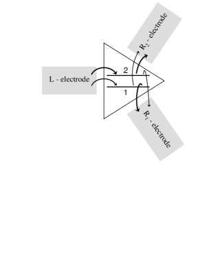
Figure 1: Schematic overview of the Y-terminal system with two level splitter, which transfers electrons from the source electrode to the two drain electrodes (from the left to the right hand side).

Let us consider a three-terminal system with a two-level QD as a splitter (presented schematically in Fig.1). The electronic transport in a sequential regime is governed by the classical master equation korotkov ; gurvitz96 ; gurvitz98

$$\frac{d}{dt}\left[\begin{array}[]{c}p_{3}\\ p_{2}\\ p_{1}\\ p_{0}\end{array}\right]=\hat{M}\left[\begin{array}[]{c}p_{3}\\ p_{2}\\ p_{1}\\ p_{0}\end{array}\right]\;,$$ (9)

where $p_{0}$, $p_{1}$, $p_{2}$ and $p_{3}$ denote probabilities of finding an empty system, a system with one electron at the level $E_{1}$ or at the level $E_{2}$, and a probability of a system with two electrons, respectively. The matrix $\hat{M}$ is given by

$$\hat{M}=\left[\begin{array}[]{cccc}-\Gamma^{31}-\Gamma^{32}&\Gamma^{23}&\Gamma^{13}&0\\ \Gamma^{32}&-\Gamma^{20}-\Gamma^{23}&0&\Gamma^{02}\\ \Gamma^{31}&0&-\Gamma^{10}-\Gamma^{13}&\Gamma^{01}\\ 0&\Gamma^{20}&\Gamma^{10}&-\Gamma^{01}-\Gamma^{02}\\ \end{array}\right]\;,$$ (14)

where $\Gamma^{nm}$ is the tunneling rate, which changes the occupation of the splitter from the state $n$ to $m$, $\Gamma^{nm}=\sum_{\alpha}\Gamma^{nm}_{\alpha}$, and $\Gamma^{nm}_{\alpha}=f_{\alpha,n}^{\pm}\gamma^{nm}_{\alpha}$ denotes the total tunneling rate from the $\alpha$ electrode ($\alpha=L$, $R_{1}$, $R_{2}$). $\gamma^{nm}_{\alpha}$ is the net tunneling rate through the $\alpha$ tunnel junction, $f^{\pm}_{\alpha,n}=1/\{1+\exp[\pm(E_{n}-\mu_{\alpha})/k_{B}T]\}$, the sign $+$ (or $-$) is for a transfer an electron from (or to) the electrode, and $\mu_{\alpha}$ denotes the chemical potential in the ${\alpha}$ electrode. We assume that the energy levels $E_{1}<E_{2}$, and when two electrons occupy the splitter, the corresponding energy is $E_{3}=E_{1}+E_{2}+U_{12}$, which includes the electron-electron repulsion energy $U_{12}$.

The current from the $\alpha$-th electrode is given by

$$I_{\alpha}\equiv I_{\alpha}^{+}-I_{\alpha}^{-}=e\sum_{n<m}(\Gamma^{nm}_{\alpha}p_{m}-\Gamma^{mn}_{\alpha}p_{n})\;.$$ (15)

(The electronic charge in our notation is taken as $e$.) The probabilities $p_{n}$ at the stationary state are determined from the master equation (9)-(14) with the left hand side equal to zero.

In the sequential regime, it is assumed that tunneling events are independent, corresponding tunneling resistances $R^{nm}_{\alpha}\gg R_{Q}=h/2e^{2}$, and the electronic transport is dominated by sequential tunneling processes averin ; schon , whereas higher order processes (cotunneling) are neglected. Moreover, it is assumed that the resonant current peak for each energy level (described by the Breit-Wigner formula) is strongly broadened by temperature; i.e., $h\gamma^{nm}_{\alpha}\ll k_{B}T$. Comparing our results on the shot noise with an experiment, one has to extract a thermal noise contribution, which is always present in any conductor (e.g., see [dicarlo, ] for thermal calibration procedure of an experimental setup).

Fluctuations in the system are studied within the generation-recombination approach for multi-electron channels. vliet ; korotkov The Fourier transform of the correlation function of the quantity $X$ and $Y$ can be expressed as korotkov

$$S_{XY}(\omega)\equiv 2\int_{-\infty}^{\infty}dte^{i\omega t}\left[\langle X(t)Y(0)\rangle-\langle X\rangle\langle Y\rangle\right]=4\sum_{n,m=0,1,2,3}X_{n}\left[P_{nm}(\omega)-\frac{p_{n}}{i\omega}\right]Y_{m}p_{m}\;,$$ (16)

where $p_{n}$ is the stationary value, $X_{n}$, and $Y_{n}$ are the values of $X$ and $Y$ at this state. The conditional probability $P(n,m;t)$ to find the system in the state $n$ at time $t$, if it was in the initial state $m$ at $t=0$, satisfies the master equation (9), vliet ; korotkov and its Fourier transform is given by $P(n,m;\omega)=[i\omega\hat{1}-\hat{M}]^{-1}_{nm}$. The elements of the Green’s function

$$G(n,m;\omega)\equiv[i\omega\hat{1}-\hat{M}]^{-1}_{nm}-p_{n}/i\omega$$ (17)

can be determined directly by matrix inversion. It is useful to perform spectral decomposition, and analyze fluctuations corresponding to characteristic eigenfrequencies. Therefore, the Green function (17) is represented by its eigenvalues $\lambda_{\nu}$ and the corresponding matrix of eigenvectors $\hat{R}$ as

$$\hat{G}=\sum_{\lambda_{\nu}}\hat{R}^{-1}\frac{-\lambda_{\nu}\hat{1}}{\omega^{2}+\lambda_{\nu}^{2}}\hat{R}\;.$$ (18)

The correlation function between the currents $I_{\alpha}$ and $I_{\alpha^{\prime}}$ can be written in the form korotkov

$$S_{\alpha\alpha^{\prime}}(\omega)=\delta_{\alpha,\alpha^{\prime}}S^{Sch}_{\alpha}+S^{c}_{\alpha\alpha^{\prime}}(\omega)\;,$$ (19)

where

$$S^{Sch}_{\alpha}\equiv 2e(I^{+}_{\alpha}+I^{-}_{\alpha})=2e^{2}\sum_{n<m}(\Gamma^{nm}_{\alpha}p_{m}+\Gamma^{mn}_{\alpha}p_{n})\;$$ (20)

is the high frequency ($\omega\to\infty$) limit of the shot-noise (the Schottky noise). The frequency-dependent part is expressed as korotkov

$$S^{c}_{\alpha\alpha^{\prime}}(\omega)=\pm 2e^{2}\{\sum_{n,m}[\Gamma^{mm+1}_{\alpha}-\Gamma^{mm-1}_{\alpha}]G_{mn}(\omega)[\Gamma^{n-1n}_{\alpha^{\prime}}p_{n-1}-\Gamma^{n+1n}_{\alpha^{\prime}}p_{n+1}]$$

$$+\sum_{n,m}[\Gamma^{mm+1}_{\alpha^{\prime}}-\Gamma^{mm-1}_{\alpha^{\prime}}]G_{mn}(-\omega)[\Gamma^{n-1n}_{\alpha}p_{n-1}-\Gamma^{n+1n}_{\alpha}p_{n+1}]\}\;,$$ (21)

where the sign ($+$) is for the cross-correlation function between the currents in the source and the drain electrode, the sign ($-$) is for the case with both currents in the drain electrodes or in the source electrode.

All results for the currents and the correlation functions can be derived analytically using a symbolic mathematical program. A problem is presentation of the results, because the formulae can be very complex. Below, we present the results for few interesting cases from a physical point of view.

II.2 Medium voltage range - Two levels in the voltage window

We consider the case of a moderate source-drain voltage $V$, for which two energy levels $E_{1}$ and $E_{2}$ lie in the voltage window, but the level $E_{3}$ is beyond the voltage window range and it does not participate in transport. Electrons can be transferred only from the left to the right hand side in Fig.1 and backflow is ignored. Nonzero elements for the total tunneling rates are: $\Gamma^{01}_{L}=\gamma^{01}_{L}$, $\Gamma^{02}_{L}=\gamma^{02}_{L}$, $\Gamma^{10}_{R_{1}}=\gamma^{10}_{R_{1}}$, $\Gamma^{20}_{R_{1}}=\gamma^{20}_{R_{1}}$, $\Gamma^{10}_{R_{2}}=\gamma^{10}_{R_{2}}$, $\Gamma^{20}_{R_{2}}=\gamma^{20}_{R_{2}}$. We ignore smearing of the Fermi distribution function $f^{\pm}_{\alpha,n}$ and they are taken equal to 1 or 0, respectively, in the expressions for the total tunneling rates $\Gamma^{nm}_{\alpha}$. In this voltage regime the Schottky term $S^{Sch}_{\alpha}$ [Eq.(20)] is equal to the Poissonian value. However, for lower voltages or higher temperatures, when backflow is allowed, $S^{Sch}_{\alpha}$ increases and can lead to the super-Poissonian shot noise.bb99 ; bb00 ; safonov In this paper we focus only on dynamical processes, which can lead to an enhancement of shot noise seen in the term $S^{c}_{\alpha\alpha^{\prime}}(\omega)$ [Eq.(II.1)]. Therefore, our studies are restricted to the case $h\gamma^{nm}_{\alpha}\ll k_{B}T\ll eV$. In this regime one can find analytical solutions and can easily extract various processes contributing to shot noise.

Let us begin with a simplest case, when the transfer rates to/from the states $E_{1}$ and $E_{2}$ are equal, i.e. $\gamma^{01}_{L}=\gamma^{02}_{L}=\gamma_{L}$, $\gamma^{10}_{R_{1}}=\gamma^{20}_{R_{1}}=\gamma_{R_{1}}$, $\gamma^{10}_{R_{2}}=\gamma^{20}_{R_{2}}=\gamma_{R_{2}}$. The current and the correlation functions at $\omega=0$ can be expressed as

$$I_{R_{1}}=\frac{2e\gamma_{L}\gamma_{R_{1}}}{2\gamma_{L}+\gamma_{R_{1}}+\gamma_{R_{2}}}\;,$$ (22)

$$S_{R_{1},R_{1}}(0)=2e|I_{R_{1}}|\;\left[1-\frac{4\gamma_{L}\gamma_{R_{1}}}{(2\gamma_{L}+\gamma_{R_{1}}+\gamma_{R_{2}})^{2}}\right]\;,$$ (23)

$$S_{R_{1},R_{2}}(0)=\frac{-16e^{2}\gamma_{L}^{2}\gamma_{R_{1}}\gamma_{R_{2}}}{(2\gamma_{L}+\gamma_{R_{1}}+\gamma_{R_{2}})^{3}}\;.$$ (24)

As one could expect anti-bunching processes dominate in this system. The auto-correlation function $S_{R_{1},R_{1}}(0)$, for the currents in the drain electrodes, is always reduced, and the cross-correlation function $S_{R_{1},R_{2}}(0)$ is always negative.

Now we consider an ideal splitter, i.e. the case when an electron can be transferred only from the level $E_{1}$ to the $R_{1}$ electrode, but transfer from this level to the $R_{2}$ electrode is forbidden, and similarly, for transfers from the level $E_{2}$, which can be realized to the $R_{2}$ electrode only. Thus, the nonzero tunneling rates are: $\gamma^{10}_{R_{1}}=\gamma_{R_{1}}$, $\gamma^{20}_{R_{2}}=\gamma_{R_{2}}$ and the transfer rates from the source electrode are still kept the same $\gamma^{01}_{L}=\gamma^{02}_{L}=\gamma_{L}$. The current, the auto- and the cross-correlation function are expressed as

$$I_{R_{1}}=I_{R_{2}}=\frac{e\gamma_{L}\gamma_{R_{1}}\gamma_{R_{2}}}{\gamma_{L}\gamma_{R_{1}}+\gamma_{L}\gamma_{R_{2}}+\gamma_{R_{1}}\gamma_{R_{2}}}\;,$$ (25)

$$S_{R_{1},R_{1}}(0)=2e|I_{R1}|\left\{1-\frac{2\gamma_{L}\gamma_{R_{1}}[\gamma_{R_{2}}(\gamma_{L}+\gamma_{R_{2}})-\gamma_{L}\gamma_{R_{1}}]}{(\gamma_{L}\gamma_{R_{1}}+\gamma_{L}\gamma_{R_{2}}+\gamma_{R_{1}}\gamma_{R_{2}})^{2}}\right\}\;,$$ (26)

$$S_{R_{1},R_{2}}(0)=\frac{-2e^{2}\gamma_{L}^{2}\gamma_{R_{1}}\gamma_{R_{2}}[\gamma_{R_{1}}\gamma_{R_{2}}(\gamma_{R_{1}}+\gamma_{R_{2}})-\gamma_{L}(\gamma_{R_{1}}-\gamma_{R_{2}})^{2}]}{(\gamma_{L}\gamma_{R_{1}}+\gamma_{L}\gamma_{R_{2}}+\gamma_{R_{1}}\gamma_{R_{2}})^{3}}\;.$$ (27)

At $\omega=0$ the current conservation is fulfilled and one can derive all other correlation functions using Eq.(25)-(27), e.g. $S_{R_{1}L}(0)=S_{R_{1}R_{1}}(0)+S_{R_{1}R_{2}}(0)$.

Although the tunneling rates $\gamma_{R_{1}}$ and $\gamma_{R_{2}}$ are different, the currents (25) in both the drain electrodes are the same (as it should be for an ideal splitter). The effect is due to dynamical Coulomb blockade, the process which distributes electrons to both the electrodes with the same probability. From Eq.(26) one can determine a condition $\gamma_{L}(\gamma_{R_{1}}-\gamma_{R_{2}})>\gamma_{R_{2}}^{2}$ for the super-Poissonian shot noise in the $R_{1}$ electrode. Positive cross-correlation between the currents in the drain electrodes $R_{1}$ and $R_{2}$ are for $\gamma_{L}(\gamma_{R_{1}}-\gamma_{R_{2}})^{2}>\gamma_{R_{1}}\gamma_{R_{2}}(\gamma_{R_{1}}+\gamma_{R_{2}})$. Both conditions are fulfilled for large asymmetry between the outgoing channels, i.e. for tunneling rates $\gamma_{R_{1}}\gg\gamma_{R_{2}}$.

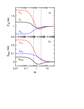
Figure 2: (Color online) Frequency dependence of the Fano factors $F_{L}$, $F_{R_{1}}$, $F_{R_{2}}$ (black, red, blue curves) - Fig.a, and the current cross-correlation functions $S_{R_{1}R_{2}}$, $S_{LR_{1}}$, $S_{LR_{2}}$ (black, red, blue curves) - Fig.b, for a medium voltage window in the Y-terminal system with an ideal two level splitter [for the transfer rates $\gamma_{L}=5$, $\gamma_{R_{1}}=1$, $\gamma_{R_{2}}=0.5$, for which the inverse of the relaxation time is $1/\tau=0.74$ and 10.75 (vertical dashed lines)]. The electron charge is taken as $e=-1$ in all our presentations.

In order to have an insight into dynamical processes leading to super-Poissonian shot noise and positive cross correlations we perform a frequency analysis of the auto- and cross-correlation functions. Fig.2 presents the results for a large asymmetry between the tunneling rates in the outgoing channels. The zero-frequency of the Fano factors $F_{R_{1}}(0)$, $F_{L}(0)>1$ and the cross-correlations $S_{R_{1}R_{2}}(0)$, $S_{LR_{1}}(0)$, $S_{LR_{2}}(0)$ are positive. It is clearly seen that all correlation functions have two contributions corresponding to two dynamical processes with characteristic frequencies $\lambda_{1}=0.74$ and $\lambda_{2}=10.75$. For most of the correlation functions the low frequency process leads to an enhancement of the auto- and the cross-correlation function, whereas the high frequency process gives a negative contribution. An exception is $S_{L,R_{2}}(\omega)$, for which the lower frequency component is negative and the high frequency contribution is positive. It means that various dynamical processes can occur in a system with electron-electron interactions, which can lead to bunching or anti-bunching. The bunching process is generally for lower frequency fluctuations, but in some cases higher frequency fluctuations can lead to bunching as well.

II.3 Three levels in the voltage window

Now we consider a large voltage regime, for which three energy levels $E_{1}$, $E_{2}$ and that one $E_{3}=E_{1}+E_{2}+U_{12}$ for two electrons in QD, are in the voltage window and all of them participate in transport. The results are presented for an ideal splitter, i.e. when an electron can be only transferred from $E_{1}$ to the $R_{1}$ electrode, from $E_{2}$ to the $R_{2}$ electrode and transfer from the $L$ electrode to all three levels is with the same tunneling rate. For this case the nonzero tunneling rates are: $\gamma^{10}_{R_{1}}=\gamma^{32}_{R_{1}}=\gamma_{R_{1}}$, $\gamma^{20}_{R_{2}}=\gamma^{31}_{R_{2}}=\gamma_{R_{2}}$ and $\gamma^{01}_{L}=\gamma^{02}_{L}=\gamma^{13}_{L}=\gamma^{23}_{L}=\gamma_{L}$. The current and the correlation functions are expressed by

$$I_{R_{1}}=\frac{e\gamma_{L}\gamma_{R_{1}}}{\gamma_{L}+\gamma_{R_{1}}}\;,$$ (28)

$$S_{R_{1},R_{1}}(\omega)=2e|I_{R_{1}}|\left[1-\frac{2\gamma_{L}\gamma_{R_{1}}}{\omega^{2}+(\gamma_{L}+\gamma_{R_{1}})^{2}}\right]\;,$$ (29)

$$S_{R_{1},R_{2}}(\omega)=0\;.$$ (30)

The current $I_{R_{2}}$ can be derived from (28) exchanging $\gamma_{R_{1}}$ and $\gamma_{R_{2}}$, and $I_{L}=I_{R_{1}}+I_{R_{2}}$. Eq.(28) suggests that $I_{R_{1}}$ is independent of the tunneling rate $\gamma_{R_{2}}$ and of the current $I_{R_{2}}$ in the second drain electrode. Indeed both the currents are independent, which one can see from Eq.(30) for the cross-correlation function $S_{R_{1},R_{2}}(\omega)=0$. These formulae (28)-(30) are much simpler than those (25)-(27) for the two levels in the voltage window (when double occupancy of the splitter is forbidden). From comparison of these two cases and one see a role of strong correlations in bunching of electrons and enhancement of the auto- and the cross-correlation functions.

Naively one could expect that shot noise should increase for the splitter with an increase of a number of levels, due to an increase of fluctuations through new tunneling channels. A spectral decomposition analysis helps us to understand a relation between fluctuations and their contribution to the correlations functions. Using (18) for the Green function we can express

$$S_{R_{1},R_{1}}(\omega)=2e|I_{R_{1}}|\left[1-\sum_{\lambda_{\nu}}\frac{s_{R_{1},R_{1}}(\lambda_{\nu})}{\omega^{2}+\lambda_{\nu}^{2}}\right]\;,$$ (31)

where the eigenfrequencies are: $\lambda_{1}=\gamma_{L}+\gamma_{R_{1}}$, $\lambda_{2}=\gamma_{L}+\gamma_{R_{2}}$, and $\lambda_{3}=2\gamma_{L}+\gamma_{R_{1}}+\gamma_{R_{2}}$. The coefficients are $s_{R_{1},R_{1}}(\lambda_{1})=2\gamma_{L}\gamma_{R_{1}}$, and $s_{R_{1},R_{1}}(\lambda_{2})=s_{R_{1},R_{1}}(\lambda_{3})=0$. We separate tunneling processes through the level $E_{1}$ and $E_{3}$ in the current $I_{R_{1}}(t)=I_{R_{1}}^{(1)}(t)+I_{R_{1}}^{(3)}(t)$. The coefficients are written in the form

$$s_{R_{1},R_{1}}(\lambda_{\nu})=s^{(11)}_{R_{1},R_{1}}(\lambda_{\nu})+2s^{(13)}_{R_{1},R_{1}}(\lambda_{\nu})+s^{(33)}_{R_{1},R_{1}}(\lambda_{\nu})\;,$$ (32)

where $s^{(nm)}_{R_{1},R_{1}}(\lambda_{\nu})$ are the coefficients corresponding to the current-current correlation functions through the levels $n,m=1,3$. Derivations are not complex, and we get $s^{(11)}_{R_{1},R_{1}}(\lambda_{1})=\gamma_{R_{1}}\gamma_{R_{2}}^{2}\gamma_{L}/(\gamma_{R_{2}}+\gamma_{L})^{2}$, $s^{(11)}_{R_{1},R_{1}}(\lambda_{2})=-\gamma_{R_{1}}\gamma_{R_{2}}\gamma_{L}^{2}/[(\gamma_{R_{1}}+\gamma_{L})(\gamma_{R_{2}}+\gamma_{L})]$, $s^{(11)}_{R_{1},R_{1}}(\lambda_{3})=\gamma_{R_{1}}\gamma_{R_{2}}\gamma_{L}^{2}(\gamma_{R_{1}}+\gamma_{R_{2}}+2\gamma_{L})/[(\gamma_{R_{1}}+\gamma_{L})(\gamma_{R_{2}}+\gamma_{L})^{2}]$, $s^{(13)}_{R_{1},R_{1}}(\lambda_{1})=\gamma_{R_{1}}\gamma_{R_{2}}\gamma_{L}^{2}/(\gamma_{R_{2}}+\gamma_{L})^{2}$, $s^{(33)}_{R_{1},R_{1}}(\lambda_{1})=\gamma_{R_{1}}\gamma_{L}^{3}/(\gamma_{R_{2}}+\gamma_{L})^{2}$. Moreover, the coefficients $s^{(11)}_{R_{1},R_{1}}(\lambda_{2})=-s^{(13)}_{R_{1},R_{1}}(\lambda_{2})=s^{(33)}_{R_{1},R_{1}}(\lambda_{2})$ and $s^{(11)}_{R_{1},R_{1}}(\lambda_{3})=-s^{(13)}_{R_{1},R_{1}}(\lambda_{3})=s^{(33)}_{R_{1},R_{1}}(\lambda_{3})$ for the eigenfrequencies $\lambda_{2}$ and $\lambda_{3}$, respectively. This analysis shows that for $\lambda_{2}$ and $\lambda_{3}$ the inter-level cross-correlation functions have opposite sign to the auto-correlation parts and they compensate each other. The nonzero contribution to the shot noise (29) is from the components $s^{(11)}_{R_{1},R_{1}}(\lambda_{1})$, $s^{(13)}_{R_{1},R_{1}}(\lambda_{1})$ and $s^{(33)}_{R_{1},R_{1}}(\lambda_{1})$, only. A similar analysis of the cross-correlation function $S_{R_{1},R_{2}}(\omega)$ shows total compensation of various partial correlation functions for the currents through all three levels.

II.4 Different potentials in drain electrodes

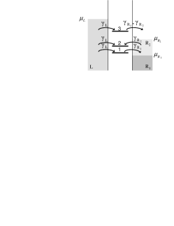
Figure 3: Schematic presentation of tunneling for the Y-terminal system with a three-level splitter and with different chemical potentials $\mu_{\alpha}$ in the $R_{1}$ and $R_{2}$ electrode. The tunneling rates, which participate in transport are presented.

In the Y-terminal system one can apply different voltages to the drain electrodes and get two different voltage windows for electron transport. Fig.3 presents a situation with a large voltage window for the $R_{1}$ electrode and a medium voltage window for the second drain electrode. Thus, an electron can tunnel from QD to the $R_{1}$ electrode from $E_{3}$ and $E_{1}$. Tunneling to the $R_{2}$ electrode can be only from $E_{3}$ (only when two electrons occupy QD); tunneling from the single electron state $E_{2}$ is forbidden because it lies below $\mu_{R_{2}}$. The tunneling rates are assumed to be the same as for an ideal splitter, for which the nonzero tunneling rates are: $\gamma^{01}_{L}=\gamma^{02}_{L}=\gamma^{13}_{L}=\gamma^{23}_{L}=\gamma_{L}$, $\gamma^{10}_{R_{1}}=\gamma^{32}_{R_{1}}=\gamma_{R_{1}}$, $\gamma^{02}_{R_{2}}=\gamma^{31}_{R_{2}}=\gamma_{R_{2}}$. The currents and the cross-correlation functions are expressed by

$$I_{R_{1}}=\frac{e\gamma_{L}\gamma_{R_{1}}}{\gamma_{L}+\gamma_{R_{1}}}\;,$$ (33)

$$I_{R_{2}}=\frac{e\gamma_{L}^{2}\gamma_{R_{2}}}{(\gamma_{L}+\gamma_{R_{1}})(\gamma_{L}+\gamma_{R_{2}})}\;,$$ (34)

$$S_{R_{1},R_{2}}(0)=-\frac{2e^{2}\gamma_{L}^{2}\gamma_{R_{1}}\gamma_{R_{2}}(\gamma_{L}-\gamma_{R_{1}})}{(\gamma_{L}+\gamma_{R_{1}})^{3}(\gamma_{L}+\gamma_{R_{2}})}\;,$$ (35)

$$S_{R_{1},R_{1}}(0)=2e|I_{R_{1}}|\left[1-\frac{2\gamma_{L}\gamma_{R_{1}}}{(\gamma_{L}+\gamma_{R_{1}})^{2}}\right]\;,$$ (36)

$$S_{R_{2},R_{2}}(0)=2e|I_{R_{2}}|\Bigl{\{}1-2\gamma_{R_{2}}\bigl{[}\gamma_{R_{1}}^{3}(\gamma_{L}+\gamma_{R_{2}})^{2}+\gamma_{L}^{4}(\gamma_{R_{2}}+2\gamma_{L})+\gamma_{L}^{3}\gamma_{R_{1}}(\gamma_{R_{2}}+3\gamma_{L})$$

$$+\gamma_{R_{1}}^{2}\gamma_{L}(2\gamma_{R_{2}}^{2}+4\gamma_{R_{2}}\gamma_{L}+3\gamma_{L}^{2})\bigr{]}/\bigl{[}\gamma_{L}(\gamma_{L}+\gamma_{R_{1}})^{2}(\gamma_{L}+\gamma_{R_{2}})^{2}(2\gamma_{L}+\gamma_{R_{1}}+\gamma_{R_{2}})\bigr{]}\Bigr{\}}\;.$$ (37)

The current $I_{R_{1}}$ and the auto-correlation function $S_{R_{1},R_{1}}(0)$ [Eq.(33) and (35)] are the same as for the case of three levels in the voltage window [Eq.(28)-(29)] considered in the previous section. The cross-correlation function $S_{R_{1},R_{2}}(0)$ is positive for $\gamma_{R_{1}}>\gamma_{L}$. Performing spectral decomposition (18) one can see contribution of relaxation processes with characteristic eigenfrequencies: $\lambda_{1}=\gamma_{L}+\gamma_{R_{1}}$, $\lambda_{2}=\gamma_{L}+\gamma_{R_{2}}$, $\lambda_{3}=2\gamma_{L}+\gamma_{R_{1}}+\gamma_{R_{2}}$. The frequency-dependent correlation functions are

$$S_{R_{1},R_{2}}(\omega)=\frac{2e^{2}\gamma_{L}\gamma_{R_{1}}\gamma_{R_{2}}}{(\gamma_{R_{1}}-\gamma_{R_{2}})(\gamma_{R_{1}}+\gamma_{R_{2}})(2\gamma_{L}+\gamma_{R_{1}}+\gamma_{R_{2}})}$$

$$\times\left[\frac{\gamma_{R_{1}}(\gamma_{R_{1}}^{2}-\gamma_{R_{1}}\gamma_{R_{2}}+\gamma_{L}\gamma_{R_{1}}-2\gamma_{L}^{2}-3\gamma_{L}\gamma_{R_{2}})}{\omega^{2}+(\gamma_{L}+\gamma_{R_{1}})^{2}}+\frac{\gamma_{R_{2}}(\gamma_{L}+\gamma_{R_{2}})(2\gamma_{L}-\gamma_{R_{1}}+\gamma_{R_{2}})}{\omega^{2}+(\gamma_{L}+\gamma_{R_{2}})^{2}}\right]\;,$$ (38)

$$S_{R_{1},R_{1}}(\omega)=2e|I_{R_{1}}|\left[1-\frac{2\gamma_{L}\gamma_{R_{1}}}{\omega^{2}+(\gamma_{L}+\gamma_{R_{1}})^{2}}\right]\;,$$ (39)

$$S_{R_{2},R_{2}}(\omega)=2e|I_{R_{2}}|\biggl{\{}1-\frac{2\gamma_{R_{2}}}{\gamma_{L}(\gamma_{R_{1}}-\gamma_{R_{2}})(2\gamma_{L}+\gamma_{R_{1}}+\gamma_{R_{2}})}$$

$$\times\biggl{[}\frac{\gamma_{R_{1}}^{2}(\gamma_{L}+\gamma_{R2})(2\gamma_{L}+\gamma_{R_{1}})}{\omega^{2}+(\gamma_{L}+\gamma_{R_{1}})^{2}}$$

$$-\frac{\gamma_{R_{1}}^{2}(\gamma_{L}+\gamma_{R_{2}})^{2}-\gamma_{L}^{2}\gamma_{R_{2}}(2\gamma_{L}+\gamma_{R_{2}})+\gamma_{L}\gamma_{R_{1}}(\gamma_{R_{2}}^{2}+2\gamma_{L}\gamma_{R_{2}}+2\gamma_{L}^{2})}{\omega^{2}+(\gamma_{L}+\gamma_{R_{2}})^{2}}\biggr{]}\biggr{\}}\;.$$ (40)

One can see that fluctuations corresponding to the eigen-frequencies $\lambda_{1}$ and $\lambda_{2}$ only contribute to the current correlation functions. A fluctuation process with the characteristic frequency $\lambda_{3}$ is absent in these correlation functions.

III Y-terminal system with a quantum dot splitter

III.1 Mediate voltage range

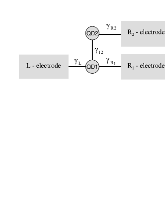
Figure 4: Schematic presentation of the Y-terminal system with two quantum dots. The net transfer rates between the quantum dots and the electrodes are shown.

Now, we consider the dynamical Coulomb blockade process in a three-terminal system connected by two quantum dots (presented schematically in Fig.4). The system is similar to two capacitatively coupled quantum dots michalek and an experimental setup zhang (see the second part of the paper [zhang, ] with a Y-terminal structure), where the sub and super-Poissonian shot noise were studied. Similarly as in the previous section, we consider sequential electronic transport, which is governed by the classical master equation korotkov ; gurvitz96 ; gurvitz98

$$\frac{d}{dt}\left[\begin{array}[]{c}p_{2}\\ p_{1}\\ p_{0}\end{array}\right]={\hat{M}}\;\left[\begin{array}[]{c}p_{2}\\ p_{1}\\ p_{0}\end{array}\right],$$ (47)

where

$$\hat{M}=\left[\begin{array}[]{ccccc}-\gamma_{R_{2}}&\gamma_{12}&0\\ 0&-\gamma_{12}-\gamma_{R_{1}}&\gamma_{L}\\ \gamma_{R_{2}}&\gamma_{R_{1}}&0&-\gamma_{L}\end{array}\right]\;.$$ (51)

Here, $p_{0}$, $p_{1}$ and $p_{2}$ denote probabilities finding an empty system, a system with one electron either at the quantum dot (QD1) or (QD2). The applied voltage difference to the left and the right electrodes is assumed to be moderate, and therefore, electron transfers are only from left to right and given by the net transfer rates shown in Fig.4. Moreover, it is assumed that only one electron can be at the splitter, either at QD1, or QD2, and $p_{2}+p_{1}+p_{0}=1$.

The currents flowing into the right electrodes are given by

$$I_{R_{1}}=e\gamma_{R_{1}}p_{1}=\frac{e\gamma_{L}\gamma_{R_{1}}\gamma_{R_{2}}}{w}\;,$$ (52)

$$I_{R_{2}}=e\gamma_{R_{2}}p_{2}=\frac{e\gamma_{L}\gamma_{12}\gamma_{R_{2}}}{w}\;,$$ (53)

where $w=\gamma_{L}\gamma_{12}+\gamma_{L}\gamma_{R_{2}}+\gamma_{12}\gamma_{R_{2}}+\gamma_{R_{1}}\gamma_{R_{2}}$. For $\gamma_{12}=\gamma_{R_{1}}$ the current $I_{R_{1}}=I_{R_{2}}$ and the system of two QD acts as an ideal splitter (for any value of $\gamma_{R_{2}}$ and $\gamma_{L}$).

The current-current correlation functions can be written as korotkov

$$S_{\alpha,\alpha^{\prime}}(\omega)=\delta_{\alpha,\alpha^{\prime}}2eI_{\alpha}+S^{c}_{\alpha,\alpha^{\prime}}(\omega)\;,$$ (54)

where the frequency dependent parts are

$$S^{c}_{LL}(\omega)=4e^{2}\;\gamma_{L}\mathrm{Re}[G_{01}(\omega)]\gamma_{L}p_{0}\;,$$ (55)

$$S^{c}_{R_{1}R_{1}}(\omega)=4e^{2}\;\gamma_{R_{1}}\mathrm{Re}[G_{10}(\omega)]\gamma_{R_{1}}p_{1}\;,$$ (56)

$$S^{c}_{R_{2}R_{2}}(\omega)=4e^{2}\;\gamma_{R_{2}}\mathrm{Re}[G_{20}(\omega)]\gamma_{R_{2}}p_{2}$$ (57)

for the auto-correlation functions and

$$S_{LR_{1}}(\omega)=2e^{2}\left\{\gamma_{L}\mathrm{Re}[G_{00}(\omega)]\gamma_{R_{1}}p_{1}+\gamma_{R_{1}}\mathrm{Re}[G_{11}(\omega)]\gamma_{L}p_{0}\right\}\;,$$ (58)

$$S_{LR_{2}}(\omega)=2e^{2}\left\{\gamma_{L}\mathrm{Re}[G_{00}(\omega)]\gamma_{R_{2}}p_{2}+\gamma_{R_{2}}\mathrm{Re}[G_{21}(\omega)]\gamma_{L}p_{0}\right\}\;,$$ (59)

$$S_{R_{1}R_{2}}(\omega)=2e^{2}\left\{\gamma_{R_{1}}\mathrm{Re}[G_{10}(\omega)]\gamma_{R_{2}}p_{2}+\gamma_{R_{2}}\mathrm{Re}[G_{20}(\omega)]\gamma_{R_{1}}p_{1}\right\}\;.$$ (60)

for the cross-correlation functions. From Eqs.(55)-(57) one can see that the autocorrelation functions $S_{\alpha\alpha}$ are proportional to the current $I_{\alpha}$ [Eq.(52)-(53)]. The factor $F_{\alpha}=S_{\alpha\alpha}/2eI_{\alpha}$ is known as the Fano factor. The cross-correlation functions $S_{\alpha\alpha^{\prime}}$ [Eq.(58)-(60)] have two terms proportional to the current $I_{\alpha}$ and $I_{\alpha^{\prime}}$, respectively. One can not extract a single factor proportional neither to the current $I_{\alpha}$, nor $I_{\alpha^{\prime}}$, nor $\sqrt{I_{\alpha}I_{\alpha^{\prime}}}$. It is not possible to define the Fano factor for the cross-correlation functions [see also Eq.(64) for $S_{R_{1}R_{2}}$ presented below]. In the literature  cottetprb ; sanchez ; vaseghi different normalizations of the cross-correlation noise were used and they were called the Fano factor, but in our opinion they have no physical meaning.

At the zero frequency limit the Fano factors for the auto-correlation functions are given by

$$F_{L}=1+2\gamma_{L}^{2}\gamma_{12}\gamma_{R_{1}}/w^{2}-2\gamma_{L}\gamma_{R_{2}}\bigl{[}\gamma_{12}(\gamma_{L}+\gamma_{12}+\gamma_{R_{1}}+\gamma_{R_{2}})+\gamma_{R_{1}}\gamma_{R_{2}}\bigr{]}/w^{2}\;,$$ (61)

$$F_{R_{1}}=1+2\gamma_{L}\gamma_{R_{1}}(\gamma_{L}\gamma_{12}-\gamma_{R_{2}}^{2})/w^{2}\;,$$ (62)

$$F_{R_{2}}=1-2\gamma_{L}\gamma_{12}\gamma_{R_{2}}(\gamma_{L}+\gamma_{12}+\gamma_{R_{1}}+\gamma_{R_{2}})/w^{2}\;.$$ (63)

In these formulae (61)-(63) we extracted positive and negative terms responsible for the super-Poissonian and the sub-Poissonian shot noise. From Eq.(62) one can easily see that $F_{R_{1}}$ is in the super-Poissonian regime, if the transfer rate $\gamma_{R_{2}}$ is small, and when one can expect a large charge accumulation at QD2. Fig.5a presents that the Fano factor $F_{L}$ is also larger than unity at small $\gamma_{R_{2}}$. The factor $F_{R_{2}}<1$ for any transfer rates. It is clear that dynamical Coulomb blockade does not occur in the $R_{2}$ channel and shot noise is always the sub-Poissonian type. The reduction of $F_{R_{2}}$ can be substantial, and it can drop to the minimal value $F_{R_{2}}=1/3$ for $\gamma_{L}=\gamma_{12}=\gamma_{R_{2}}$ and $\gamma_{R_{1}}\to 0$ [see Eq.(63)]. It is well known that the Fano factor in sequential transport through a quantum dot may be reduced to its minimal value $F=1/2$. korotkov92 ; hershfield ; korotkov ; blanter In the present case, however, the system is with two quantum dots connected in series. In the Appendix we show that the shot noise reduction can be even larger for a system with a large number of quantum dots. The exact calculations show that in a system of $N$ quantum dots connected in series the Fano factor can be reduced to the value $F=1/(N+1)$.

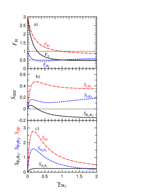
Figure 5: (Color online) Plot of the Fano factors $F_{\alpha}$ (for the $L$-, $R_{1}$ and $R_{2}$ electrodes - black, red and blue curve, respectively) – Fig.a; the current cross-correlation functions $S_{\alpha\alpha^{\prime}}$ ($S_{R_{1}R_{2}}$ - black, $S_{LR_{1}}$ - red and $S_{LR_{2}}$ - blue) – Fig.b; and the potential correlation functions $S_{\phi_{1}\phi_{1}}$, $S_{\phi_{2}\phi_{2}}$ (black and blue) as well as the polarization correlation function $S_{pp}$ (red) – Fig.c, as a function of the transfer rate $\gamma_{R_{2}}$ at the zero-frequency $\omega=0$. The other transfer rates are: $\gamma_{L}=\gamma_{12}=\gamma_{R_{1}}=1$.

Using the formulae (58)-(60) one can derive the cross-correlations functions. Below we present the function

$$S_{R_{1}R_{2}}(0)=-2I_{R_{1}}I_{R_{2}}(\gamma_{L}+\gamma_{12}+\gamma_{R_{1}}+2\gamma_{R_{2}})/w+2e^{2}\gamma_{L}^{3}\gamma_{12}^{2}\gamma_{R_{1}}\gamma_{R_{2}}/w^{3}\;.$$ (64)

At $\omega=0$ the current conservation is fulfilled and we can derive all other cross-correlation functions using Eq.(61)-(64), e.g. $S_{LR_{1}}(0)=S_{R_{1}R_{1}}(0)+S_{R_{2}R_{1}}(0)$, $S_{LR_{2}}(0)=S_{R_{1}R_{2}}(0)+S_{R_{2}R_{2}}(0)$. Fig.5b presents the results for the cross-correlation functions. All of them show a peak at a small $\gamma_{R_{2}}$. Increasing the tunneling rate $\gamma_{R_{2}}$ the correlation function $S_{R_{1}R_{2}}$ decreases and changes its sign. It suggests that bunching processes weaken their intensity and antibunching becomes dominating.

Bunching effects and super-Poissonian noise are caused by dynamical Coulomb blockade, which should be seen in charge and potential fluctuations in the system (especially at QD2). If we denote a local potential $\phi_{i}(t)=\phi_{0}+en_{i}(t)$ depending on fluctuation of the number of electrons $n_{i}(t)$ at the i-th quantum dot, then using Eq.(16) one can write the potential-potential correlation function

$$S_{\phi_{i}\phi_{i}}(0)\equiv 4\sum_{n,m}\phi_{i}(n)\mathrm{Re}[G_{nm}(0)]\phi_{i}(m)p_{m}=4e^{2}\mathrm{Re}[G_{ii}(0)]p_{i}\;.$$ (65)

Fig.5c shows that the potential fluctuations $S_{\phi_{2}\phi_{2}}$ at QD2 are large in the region of small values of $\gamma_{R_{2}}$. In Fig.5c we plotted the correlation function $S_{pp}$ for the polarization $p(t)=\phi_{2}(t)-\phi_{1}(t)$ between the charges localized at QD1 and QD2. The corresponding curve (red) presents very large fluctuations in the same region of the parameters as the super-Poissonian shot noise. Note that $S_{\phi_{1}\phi_{1}}$ monotonically increases and it does not show activation of any potential fluctuations at small $\gamma_{R_{2}}$.

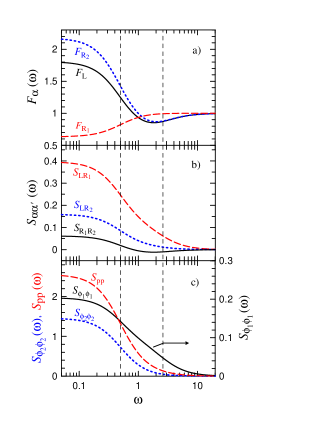
Figure 6: (Color online) Frequency dependence of the Fano factors $F_{L}$, $F_{R_{1}}$, $F_{R_{2}}$ (black, red, blue curves) - Fig.a; the current cross-correlation functions $S_{R_{1}R_{2}}$, $S_{LR_{1}}$, $S_{LR_{2}}$ (black, red, blue curves) - Fig.b; and the potential correlation functions $S_{\phi_{1}\phi_{1}}$, $S_{\phi_{2}\phi_{2}1}$ and the polarization correlation function $S_{pp}$ (black, blue and red curves) - Fig.c. The transfer rates are: $\gamma_{L}=\gamma_{12}=\gamma_{R_{1}}=1$, $\gamma_{R_{2}}=0.1$, for which the eigen-frequency is $\lambda=0.5$ and 2.6 (vertical dashed lines).

These results suggest that a charge accumulated at QD2 influences the transport through QD1. In order to get more information on dynamics of this feedback process we perform a frequency analysis. One can do a spectral decomposition of all studied correlation functions and determine components corresponding to eigen-frequencies of the system (see eg.[bb00, ]). For the case presented in Fig.6 one gets $\lambda_{1}=0.5$ and $\lambda_{2}=2.6$. Its inverse $\tau_{\nu}=1/\lambda_{\nu}$ is a relaxation time for eigen-fluctuations in the system. A role of the corresponding relaxation processes in the range of the super-Poissonian noise is presented in Fig.6. The Fano factors $F_{L}$ and $F_{R_{2}}$ are higher than unity in the low frequency range, whereas $F_{R_{1}}$ is always below unity. It means that for $F_{L}$ and $F_{R_{2}}$ their low frequency components lead to super-Poissonian shot noise, whereas high frequency contributions reduce shot noise. For given parameters the low frequency part can dominate the high frequency contribution and a measurement should show a super-Poissonian value of a zero-frequency power spectrum. Fig.6b shows frequency-dependent plots of the cross-correlation functions. The function $S_{R_{1}R_{2}}$ clearly shows two components: low and high frequency ones. Low frequency components are positive and they dominate. It means that the low frequency process leads to the positive cross-correlation function $S_{R_{1}R_{2}}$ for outgoing electrons.

Fig.6c presents fluctuations of the polarization $S_{pp}$ and the charge fluctuations $S_{\phi_{2}\phi_{2}}$ at QD2, which occur only in the low frequency regime. The plot of the function $S_{\phi_{1}\phi_{1}}$ is different and shows that the high frequency component is also relevant in the potential fluctuations at QD1. Applying the spectral decomposition procedure we can assign the lower eigen-frequency to the polarization fluctuations. It means also that the dynamical Coulomb blockade leads to the bunching effect for electrons.

III.2 Large voltage window

In Sec.II.3, we showed that if two electron states participate in transport through a multi-level splitter, then the dynamical Coulomb blockade effect is reduced, and in a special case the cross-correlation function can be $S_{R_{1}R_{1}}(\omega)=0$. One can expect also a reduction of shot noise for the quantum dot splitter at higher voltages. In this section we consider a situation with a large voltage window when energy of second electron overcomes the Coulomb repulsion energy and the electron is introduced on an empty QD. The master equation is

$$\frac{d}{dt}\left[\begin{array}[]{c}p_{12}\\ p_{2}\\ p_{1}\\ p_{0}\end{array}\right]={\hat{M}}\;\left[\begin{array}[]{c}p_{12}\\ p_{2}\\ p_{1}\\ p_{0}\end{array}\right],$$ (74)

where

$$\hat{M}=\left[\begin{array}[]{cccc}-\gamma_{R_{1}}-\gamma_{R_{2}}&\gamma_{L}&0&0\\ \gamma_{R_{1}}&-\gamma_{L}-\gamma_{R_{2}}&\gamma_{12}&0\\ \gamma_{R_{2}}&0&-\gamma_{12}-\gamma_{R_{1}}&\gamma_{L}\\ 0&\gamma_{R_{2}}&\gamma_{R_{1}}&-\gamma_{L}\end{array}\right]\;,$$ (79)

and $p_{12}$ is the probability to find simultaneously two electrons at QD1 and QD2. The currents flowing into the right electrodes are

$$I_{R_{1}}=\frac{e\gamma_{L}\gamma_{R_{1}}(\gamma_{R_{1}}\gamma_{R_{2}}+\gamma_{R_{2}}^{2}+\gamma_{L}\gamma_{12}+\gamma_{L}\gamma_{R_{2}})}{w}\;,$$ (80)

$$I_{R_{2}}=\frac{e\gamma_{L}\gamma_{12}\gamma_{R_{2}}(\gamma_{L}+\gamma_{R_{1}}+\gamma_{R_{2}})}{w}\;,$$ (81)

where $w=\gamma_{R_{2}}(\gamma_{R_{1}}+\gamma_{L})(\gamma_{R_{1}}+\gamma_{R_{2}}+\gamma_{L})+\gamma_{12}[\gamma_{R_{2}}^{2}+\gamma_{R_{2}}\gamma_{L}+\gamma_{L}^{2}+\gamma_{R_{1}}(\gamma_{R_{2}}+\gamma_{L})]$. When the two electron state $(1,1)$ participates in transport the currents increase [compare Eq.(80)-(81) with Eq.(52)-(53)], but their enhancement is different for the different drain electrodes. In previous section we have seen that the system acts as an ideal current splitter (with $I_{R_{1}}=I_{R_{2}}$) for $\gamma_{12}=\gamma_{R_{1}}$. Now, because single and two electron states are in the voltage window, ideal current redistribution is broken (in general, $I_{R_{1}}\neq I_{R_{2}}$).

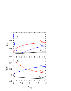
Figure 7: (Color online) Plot of the Fano factors $F_{\alpha}$ (for the $L$-, $R_{1}$ and $R_{2}$ electrodes - black, red and blue curve, respectively) – Fig.a, and the current cross-correlation functions $S_{\alpha\alpha^{\prime}}$ ($S_{R_{1}R_{2}}$ - black, $S_{LR_{1}}$ - red and $S_{LR_{2}}$ - blue) – Fig.b, as a function of the transfer rate $\gamma_{R_{2}}$ at $\omega=0$ and in the high voltage regime, when single and two electron states participate in transport. The parameters are the same as in Fig.5.

The current-current correlation functions are derived analytically in the same way as previously. Because the formulae are rather complex, we present plots of the auto- and cross-correlation functions in Fig.7. All Fano factors are in the sub-Poissonian regime. The factors $F_{L}$ and $F_{R_{2}}$ show strong reduction, which can be even below the value $F=1/2$ for a single quantum dot system. The cross-correlation function $S_{R_{1}R_{2}}$ is always negative. These results are different than those presented in Fig.5 for a mediate voltage regime, when the two electron state is outside the voltage window. Now the correlation functions do not show bunching effects – antibunching processes dominate in shot noise.

IV Summary and concluding remarks

Our study addresses dynamical aspects in current shot noise in the Y-terminal system with a multilevel splitter. We showed that the zero-frequency current-current auto- and cross-correlation functions increase because of the dynamical Coulomb blockade effect. Furthermore, the spectral decomposition analysis indicates that the dynamic Coulomb blockade effect is caused by charge fluctuations corresponding to an electron accumulated at the level with a lowest outgoing tunneling rate. This process exhibits itself a large asymmetry in the tunneling rates and strong Coulomb interactions. In the section II.B, we present the case for the Y-terminal system with an ideal two-level splitter, when an electron is transferred from a given level to only one of two drain electrodes, and with a further assumption of a single electron occupancy of the splitter. An increase of the voltage changes the situation dramatically. For a large voltage, when three levels are in the voltage window and double electron occupancy is allowed, electrons transferred to the drain electrodes behave like independent particles with the cross-correlation function $S_{R_{1},R_{2}}(\omega)=0$ (for any frequency $\omega$). Having separated the currents into the partial currents, flowing through each energy level, and using the spectral analysis, we were able to decompose the correlation functions, and determine a role of each individual component for any eigenfrequency. The partial auto-correlation functions compensate the partial cross-correlation functions, leading to $S_{R_{1},R_{2}}(\omega)=0$, and reduce the auto-correlation function $S_{R_{1},R_{1}}(\omega)$ [see Eq.(33)]. For the situation considered, bunching and antibunching scattering processes compensate each other perfectly. We also considered the case with different voltages applied to the drain electrons, with the voltage windows of different sizes (with three and one level in the window, respectively). The current fluctuations are then compensated only partially. For example, the cross-correlations can be positive and negative, depending on the tunneling rates for incoming and outgoing channels.

We suggest to perform an experiment to see these correlation effects on a multilevel QD system. A direct observation of the bunching process on a two-terminal multilevel QD was performed by Gustavsson et al. gustavssonprl ; gustavssonprb using a quantum point contact system acting as a charge sensor. Our proposal is different because the system should be three-terminal one with asymmetric tunnel contacts, and current cross correlation measurements should be performed. In the experiment, one has to change the voltage window, from the low to the strong voltage regime, in order to change the number of levels and the number of electrons participating in transport.

We also considered the Y-terminal system with two quantum dots, which is the model corresponding to the experimental setup recently studied by Zhang et al. zhang . In the experiment zhang , one can control all the parameters of the system, and verify our theoretical predictions. Our studies show that the dynamical Coulomb blockade effect leads to electron bunching, and the effect manifests itself with strong charge fluctuations at the side quantum dot (QD2). In order to activate the effect, one has to apply the gate voltage, and reduce the tunneling rate $\gamma_{R_{2}}$ from QD2 to the electrode. We predict an increase of the Fano factor $F_{R_{1}}$ to the super-Poissonian regime and positive cross-correlations $S_{R_{1}R_{2}}$ for $\gamma_{R_{2}}\to 0$. When the bias voltage increases, we expect that the two electron state will become a participant in transport, and shot noise will significantly be reduced to the sub-Poissonian regime. We also predict that in a system consisting of N quantum dots connected in series, a minimal value of the Fano factor is $F=1/(N+1)$.

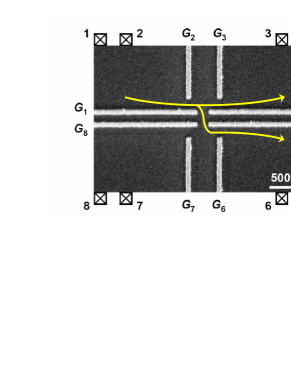
Figure 8: An experimental setup for two coupled quantum wires, which can be used for studies of shot noise and electron bunching (adapted from [bird, ]). By tuning voltages applied to the gates G$2$, G₃ and G₆, one can change tunneling transfer rates for the incoming and outgoing channels in the splitter, and test the dynamical Coulomb blockade processes in the current-current cross correlations.

We could not point out a microscopic origin of an enhancement of shot noise in the experiments on a quantum point contact chen ; zarchin . We also could not find a source of local or spatial charge (potential) fluctuations, which lead to bunching in a such simple experimental setup with a quantum point contact. We hope that dynamical Coulomb blockade is again responsible for bunching in this case. Therefore, we propose shot noise measurements in a similar system presented in Fig.8. In this case, two ballistic channels are coupled with each other, and current can be split into two electrodes, similar to the experiments in [chen, ; zarchin, ]. This experimental setup allows control of output channels by the gate electrodes G₃ and G₆, which can also control charge fluctuations in the system. We speculate that dynamical Coulomb blockade leads to bunching in coherent electron transport as well. To our best knowledge, there is no research in the coherent transport regime showing electron bunching. While there are related papers noisekondo on shot noise in the coherent regime, which take into account electron-electron interactions and the Kondo resonance, but their shot noise is in the sub-Poissonian regime.

Appendix A Current noise in quantum dots connected in series

We consider a system of $N$-quantum dots connected in series in a high voltage limit, in which electrons can only hop from left to right. The master equation can be written as

$$\frac{d}{dt}\left[\begin{array}[]{c}p_{N}\\ \vdots\\ p_{2}\\ p_{1}\\ p_{0}\end{array}\right]=\left[\begin{array}[]{cccccc}-\gamma_{NR}&\gamma_{N-1N}&...&0&0&0\\ \vdots&\vdots&\ddots&\vdots&\vdots&\vdots\\ 0&0&...&-\gamma_{23}&\gamma_{12}&0\\ 0&0&...&0&-\gamma_{12}&\gamma_{L1}\\ \ \gamma_{NR}&0&...&0&0&-\gamma_{L1}\\ \end{array}\right]\;\left[\begin{array}[]{c}p_{N}\\ \vdots\\ p_{2}\\ p_{1}\\ p_{0}\end{array}\right],$$ (97)

where we have assumed a single electron in the system, i.e. $\sum_{n}p_{n}=1$. Here, we present the analytical results for the $N=3$ system. The current is expressed as

$$I=e\frac{\gamma_{L1}\gamma_{12}\gamma_{23}\gamma_{3R}}{\gamma_{L1}\gamma_{12}\gamma_{23}+\gamma_{L1}\gamma_{12}\gamma_{3R}+\gamma_{L1}\gamma_{23}\gamma_{3R}+\gamma_{12}\gamma_{23}\gamma_{3R}}\;.$$ (98)

The zero-frequency current shot noise is given by

$$S_{LL}=S_{RR}=S_{LR}=2eI\frac{\gamma_{L1}^{2}\gamma_{12}^{2}\gamma_{23}^{2}+\gamma_{L1}^{2}\gamma_{12}^{2}\gamma_{3R}^{2}+\gamma_{L1}^{2}\gamma_{23}^{2}\gamma_{3R}^{2}+\gamma_{12}^{2}\gamma_{23}^{2}\gamma_{3R}^{2}}{(\gamma_{L1}\gamma_{12}\gamma_{23}+\gamma_{L1}\gamma_{12}\gamma_{3R}+\gamma_{L1}\gamma_{23}\gamma_{3R}+\gamma_{12}\gamma_{23}\gamma_{3R})^{2}}\;.$$ (99)

It is clear that the Fano factor $F=S/2eI\leq 1$ and its lowest value $\min\{F\}=1/4$ is reached for $\gamma_{L1}=\gamma_{12}=\gamma_{23}=\gamma_{3R}$. Generalization for any $N$ can be straightforward performed by a mathematical induction, showing that $\min\{F\}=1/(N+1)$.

This result is a generalization of the Fano factor derived for a single QD in a sequential tunneling regime, when $\min\{F\}=1/2$. korotkov92 ; hershfield ; korotkov ; blanter

References

- (1) I.O. Kulik and A.N. Omel’yanchuk, Fiz. Nizk. Temp. 10, 305 (1984) [Sov. J. Low Temp. Phys. 10, 158 (1984)].
- (2) V. A. Khlus, Zh. Eksp. Teor. Fiz. 93, 2179 (1987) [Sov. Phys. JETP 66, 1243 (1987)].
- (3) G.B. Lesovik, Pis’ma Zh. Eksp. Teor. Fiz. 49, 513 (1989) [JETP Lett. 49, 592 (1989)].
- (4) M. Büttiker, Phys. Rev. Lett. 65, 2901 (1990).
- (5) C.W.J. Beenakker and M. Büttiker, Phys. Rev. B 46, 1889 (1992).
- (6) H.U. Baranger and P.A. Mello, Phys. Rev. Lett. 73, 142 (1994).
- (7) R.A. Jalabert, J.-L. Pichard and C.W.J. Beenakker, Europhys. Lett. 27, 255 (1994).
- (8) A. N. Korotkov, D. V. Averin, K. K. Likharev and S. A. Vasenko, in Single-Electron Tunneling and Mesoscopic Devices, H. Koch, H. Lübbig (Eds.), Springer Series in Electronics and Photonics, Vol. 31, Springer, Berlin, 1992, p. 45.
- (9) S. Hershfield, J.H. Davies, P. Hyldgaard, C.J. Stanton and J.W. Wilkins, Phys. Rev. B 47, 1967 (1993).
- (10) A.N. Korotkov, Phys. Rev. B 49, 10 381 (1994).
- (11) Ya.M. Blanter and M. Büttiker, Phys. Rep. 336, 1 (2000).
- (12) G. Iannaccone, G. Lombardi, M. Macucci, and B. Pellegrini, Phys. Rev. Lett. 80, 1054 (1998); Nanotechnology 10, 97 (1999).
- (13) V.V. Kuznetsov, E.E. Mendez, J.D. Bruno, J.T. Pham, Phys. Rev. B 58, R10159 (1998).
- (14) B.R. Bułka, J. Martinek, G. Michałek and J. Barnaś, Phys. Rev. B 60, 12 246 (1999).
- (15) S.S. Safonov, A.K. Savchenko, D.A. Bagrets, O.N. Jouravlev, Y.V. Nazarov, E.H. Linfield, and D.A. Ritchie, Phys. Rev. Lett. 91, 136801 (2003).
- (16) B. R. Bułka, Phys. Rev. B 62, 1186 (2000).
- (17) G. Michałek and B.R. Bułka, Eur. Phys. J. B 28, 121 (2002).
- (18) R. Guerrero, F. G. Aliev, Y. Tserkovnyak, T. S. Santos, and J. S. Moodera, Phys. Rev. Lett. 97, 266602 (2006).
- (19) S. Garzon, Y. Chen and R.A. Webb, Physica E 40, 133 (2007).
- (20) D.T. McClure, L. DiCarlo, Y. Zhang, H.-A. Engel, C.M. Marcus, M.P. Hanson and A.C. Gossard, Phys. Rev. Lett. 98, 056801 (2007).
- (21) Y. Zhang, L. DiCarlo, D. T. McClure, M. Yamamoto, S. Tarucha, C.M. Marcus, M. P. Hanson, and A.C. Gossard, Phys. Rev. Lett. 99, 036603 (2007).
- (22) E.V. Sukhorukov, G. Burkard, and D. Loss, Phys. Rev. B 63, 125315 (2001).
- (23) A. Thielmann, M.H. Hettler, J. König, and G. Schön, Phys. Rev. Lett. 95, 146806 (2005).
- (24) R.P. Feynman, R.B. Leighton, and M. Sands, The Feynman Lectures (Addison-Wesley, Reading, 1965), Vol. 3.
- (25) R. Hanbury Brown, R.Q. Twiss, Nature 177, 27 (1956).
- (26) R.C. Liu, B. Odom, Y. Yamamoto and S. Tarucha, Nature 391, 263 (1998).
- (27) W.D. Oliver, J. Kim, R.C. Liu, and Y. Yamamoto, Science 284, 299 (1999).
- (28) M. Henny, S. Oberholzer, C. Strunk, T. Heinzel, K. Ensslin, M. Holland, C. Schönenberger, Science 284, 296 (1999).
- (29) R. Loudon, Phys. Rev. A 58, 4904 (1998).
- (30) C. Texier, M. Büttiker, Phys. Rev. B 62, 7454 (2000).
- (31) T. Martin and R. Landauer, Phys. Rev. B 45, 1742 (1992).
- (32) S. Oberholzer, E. Bieri, and C. Schönenberger, M. Giovannini and J. Faist, Phys. Rev. Lett. 96, 046804 (2006).
- (33) G. Burkard, D. Loss, and E. V. Sukhorukov, Phys. Rev. B 61, R16303 (2000).
- (34) A. Cottet, W. Belzig and C. Bruder, Phys. Rev. B 70, 115315 (2004).
- (35) A. Cottet, W. Belzig, C. Bruder, Phys. Rev. Lett. 92, 206801 (2004).
- (36) A. Cottet and W. Belzig, Europhys. Lett. 66, 405 (2004).
- (37) S. Gustavsson, R. Leturcq, B. Simovic, R. Schleser, T. Ihn, P. Studerus, and K. Ensslin, D. C. Driscoll and A.C. Gossard, Phys. Rev. Lett. 96, 076605 (2006).
- (38) S. Gustavsson, R. Leturcq, B. Simovic, R. Schleser, P. Studerus, T. Ihn, K. Ensslin, D.C. Driscoll and A.C. Gossard, Phys. Rev. B 74, 195305 (2006).
- (39) S.-T. Wu and S. Yip, Phys. Rev. B 72, 153101 (2005).
- (40) V. Rychkov and M. Büttiker, Phys. Rev. Lett. 96, 166806 (2006).
- (41) Y. Chen and R.A. Webb, Phys. Rev. Lett. 97, 066604 (2006).
- (42) O. Zarchin, Y.C. Chung, M. Heiblum, D. Rohrlich and V. Umansky, Phys. Rev. Lett. 98, 066801 (2007)
- (43) S. A. Gurvitz and Ya. S. Prager, Phys. Rev. B 53, 15932 (1996).
- (44) S. A. Gurvitz, Phys. Rev. B 57, 6602 (1998).
- (45) D.V. Averin, A.N. Korotkov, K.K. Likharev, Phys. Rev. B 44, 6199 (1991)
- (46) G. Schön, in Quantum Transport and Dissipation, edited by T. Dittrich, P. Hänggi, G.-L. Ingold, B. Kramer, G. Schön, W. Zwerger, Chap. 3 (Wiley-VCH Verlag, New York, 1998)
- (47) L. DiCarlo, Y. Zhang, D. T. McClure, C. M. Marcus, L. N. Pfeiffer and K. W. West, Rev. Sci. Instrum. 77, 073906 (2006).
- (48) K. M. van Vliet and J. R. Faset in Fluctuation Phenomena in Solids, edited by R. E. Burgess (Academic Press, New York, 1965), p.267.
- (49) D. Sánchez and R. López, Phys. Rev. B 71, 035315 (2005).
- (50) S.V. Vaseghi, Advanced Digital Signal Processing and Noise Reduction, John Willey and Sons Ltd (2000), ch.3.4.7.
- (51) Y. Yoon, L. Mourokh,T. Morimoto, N. Aoki, Y. Ochiai, J. L. Reno, and J. P. Bird, Phys. Rev. Lett. 99, 136805 (2007).
- (52) see for example: S. Hershfield, Phys. Rev. B 46, 7061 (1992); F. Yamaguchi and K. Kawamura, J. Phys. Soc. Japan 63, 1258 (1994); M. Hamasaki, Phys. Rev. B 69, 115313 (2004); D. Sanchez and R. Lopez, Phys. Rev. B 71, 035315 (2005); A. Golub, Phys. Rev. B 73, 233310 (2006); T. L. Schmidt, A. Komnik, and A. O. Gogolin, Phys. Rev. Lett. 98, 056603 (2007); and references therein.