Controlled impact of a disk on a water surface: Cavity dynamics.

Abstract

In this paper we study the transient surface cavity which is created by the controlled impact of a disk of radius $h_{0}$ on a water surface at Froude numbers below 200. The dynamics of the transient free surface is recorded by high speed imaging and compared to boundary integral simulations. An excellent agreement is found between both. The flow surrounding the cavity is measured with high speed particle image velocimetry and is found to also agree perfectly with the flow field obtained from the simulations.
We present a simple model for the radial dynamics of the cavity based on the collapse of an infinite cylinder. This model accounts for the observed asymmetry of the radial dynamics between the expansion and contraction phase of the cavity. It reproduces the scaling of the closure depth and total depth of the cavity which are both found to scale roughly as $\propto\text{Fr}^{1/2}$ with a weakly Froude number dependent prefactor. In addition, the model accurately captures the dynamics of the minimal radius of the cavity, the scaling of the volume $V_{bubble}$ of air entrained by the process, namely $V_{bubble}/h_{0}^{3}\propto(1+0.26\text{Fr}^{1/2})\text{Fr}^{1/2}$, and gives insight into the axial asymmetry of the pinch-off process.

1 Introduction

A spectacular example of free surface flow is the impact of an object on a liquid: The impact creates a splash and a transient cavity. This surface cavity then violently collapses under the influence of the hydrostatic pressure. At the singularity where the walls of the cavity collide, two powerful jets develop, one downwards and the other one upwards up to several meters high, making this fast event an impressive scene. Research into the physics of these transient surface cavities started at the beginning of the twentieth century when A.M. Worthington published his famous work ”A study of splashes” (Worthington (1908)). His photographs revealed a wealth of phenomena of unanticipated complexity (Worthington & Cole (1897)). Although much has been contributed to the understanding of these phenomena, many of the intriguing questions posed by Worthington’s photographs resonate still today (Rein (1993); Fedorchenko & Wang (2004)).

All investigations since Worthington’s studies entailed experiments with a freely falling object impacting on the free surface. To gain further insight into such impact events, we built a setup in which we attach the impacting object to a linear motor. In this way we gain full control over the impact velocity, which now turns from a response observable into the key control parameter of the system.

The dynamics of a surface cavity are of enormous practical importance in many natural and industrial processes: Raindrops falling onto the ocean entrain air (Oguz & Prosperetti (1990); Oguz et al. (1995); Prosperetti & Oguz (1997)) and it is this mechanism which is one of the major sinks of carbon dioxide from the atmosphere. Droplet impact and the subsequent void collapse are also a significant source of underwater sound (Prosperetti et al. (1989)) and a thorough understanding is therefore crucial in sonar research. High speed water impacts and underwater cavity formation are moreover of relevance to military operations (Gilbarg & Anderson (1948); Lee et al. (1997); Duclaux et al. (2007)). In the context of industrial applications, drop impact and the subsequent void formation are crucial in pyrometallurgy (Liow et al. (1996); Morton et al. (2000)), in the food industry, and in the context of ink-jet printing (Le (1998); Chen & Basaran (2002); de Jong et al. (2006a); de Jong et al. (2006b)). A similar series of events as in water can even be observed when a steel ball impacts on very fine and soft sand (Thoroddsen & Shen (2001); Lohse et al. (2004); Royer et al. (2005); Caballero et al. (2007)).

Although in some of the literature the deceleration of the impacting body was minimized by choosing the properties of the body such that the velocity of the impactor remained roughly constant during the time the cavity dynamics were observed (Glasheen & McMahon (1996); Gaudet (1998)), the velocity of the body nevertheless remained a response parameter set by the system. Our use of a linear motor to accurately control the position, velocity, and acceleration of the impacting object constitutes the key difference between our work (see also Bergmann et al. (2006); Gekle et al. (2008)) and all previous literature.

In this article, we will use observations from experiments and boundary integral simulations to construct a model which accurately describes the radial dynamics of the cavity.
In Section 2 we present results from our controlled experiment and compare them to the boundary integral simulations. More specifically, in subsection 2.3 we discuss the dynamics of the free surface and continue in subsection 2.4 with the topology and magnitude of the flow surrounding the cavity obtained by particle image velocimetry.
In Section 3 we will derive a model which captures the radial dynamics of the cavity. We will use the model to investigate the following key characteristics of the transient surface cavity: First, the depth at which the pinch-off will occur is discussed in subsection 4.1. Then, in subsection 4.2 the amount of air entrained by the cavity collapse is studied. The article is concluded in Section 5. The results from our earlier paper Bergmann et al. (2006) that are relevant to the present study are reviewed in Appendix A, together with some additional information on the time evolution of the neck radius and the cavity. Finally, Appendix B discusses the dynamics of the minimal radius within the context of the model.

2 Experimental and numerical results

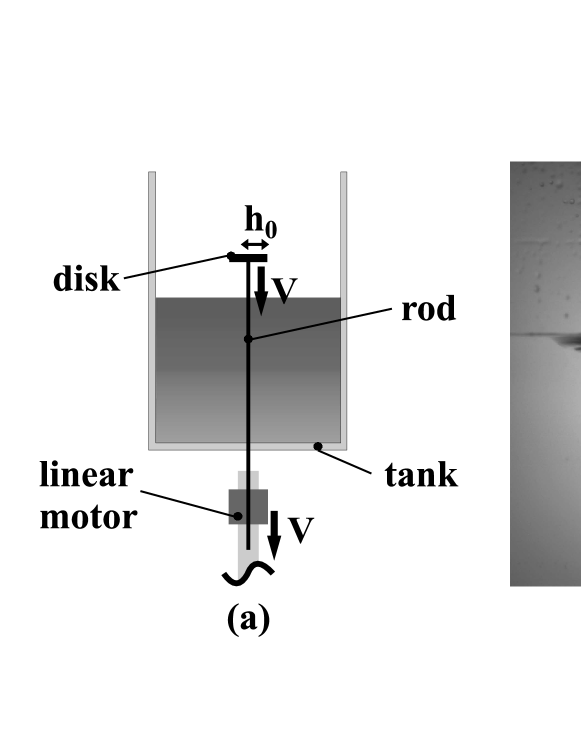
Figure 1: (a) Schematic figure of the experimental setup with the linear motor controlling the rod and disk. The vertical rod runs through a seal in the bottom of the glass water tank and is pulled down by the linear motor in order to impact the disk on the water surface. Here, $h_{0}$ is the radius and $V$ the controlled and constant velocity of the disk. (b) The formation of an upward and downward jet after the cavity has closed. In the present study we will focus on the cavity dynamics until pinch-off, just before the jet formation.

2.1 Experimental setup and procedure

A sketch of the setup is seen in Fig. 1a. A disk of radius $h_{0}$ is mounted on top of a thin rod ($\varnothing$ 6 mm). This rod runs through a seal in the bottom of a large tank (500 mm$\times$500 mm$\times$1000 mm) and is connected at the lower end to a Thrusttube linear motor which is used to determine and control the velocity and acceleration of the disk. The position of the motor (and thus of the disk) along the vertical axis is measured with a spatial accuracy of 5 $\mu$m over a range of 1 m, the large acceleration of the motor (up to 30 $g$, with $g$ the gravitational acceleration) makes it possible to perform impact experiments with constant velocities up to 5 m/s.

The effect of the small diameter of the rod on the global flow and dynamics of the cavity is assumed to be negligible. As the minimum radius for the disk used in the experiments is 10 mm, the ratio of the cross–sectional area of the rod and the surface of the disk is always smaller than 9%. Since the rod is mounted in the center of the disk, where stagnation would normally occur, the influence on the radially outward flow below the disk is presumably small.

Using the flat plate approximation, we can also estimate the direct contribution of the boundary layer of the rod to the axial flow. The boundary layer thickness $\delta$ for a flat plate is given by Blasius’ solution $\delta\approx 5\sqrt{\nu\Delta t}$, where $\nu$ is the kinematic viscosity of water and $\Delta t$ the time the boundary layer has to develop. We will equate the time $\Delta t$ to the duration of the experiment, namely to the time interval starting from the impact of the disk until the collapse of the void, which in our experiments is found to scale as $\Delta t\approx 2.5\sqrt{h_{0}/g}$, as will be discussed in detail in subsection 4.1. For the largest disk size in the experiment $h_{0}=40$ mm, this result predicts a maximum boundary layer thickness of 1.8 mm. Under most experimental conditions of this study it is considerably thinner.

In our experiments we pull the disk down with a constant velocity $V$. Making this main control parameter dimensionless, we obtain the Froude number $\text{Fr}=V^{2}/(gh_{0})$. The liquid properties are expressed in terms of the Reynolds number $\text{Re}=Vh_{0}/\nu$ and the Weber number $\text{We}=\rho V^{2}h_{0}/\sigma$, where $\sigma$ denotes the surface tension and $\rho$ the fluid density. Since the Reynolds number and the Weber number are considerable on the large scales of Fig. 1, the viscosity and the surface tension do not seem to play a role. To be more precise, in our experiment the Reynolds number ranges between 500 and $1.6\cdot 10^{4}$ and the Weber number ranges between 34 and $8.8\cdot 10^{3}$. Note however that under only slightly different conditions, namely replacing the disk by a cylinder submerged in water to avoid the splash, capillary waves do play a role (see Gekle et al. (2008)). For the impact of a disk we find the only important dimensionless parameter to be the Froude number, i.e., the ratio of kinetic to gravitational energy, which ranges from $0.6$ to $200$ in our experiments. It is convenient to use the amount of time $\tau$ remaining until cavity collapse which is given by $\tau=t-t_{coll}$ with $t_{coll}$ the collapse time.

2.2 Numerical method

The numerical calculations are performed using a boundary integral method (Prosperetti (2002); Power & Wrobel (1995); Oguz & Prosperetti (1993)) based on potential flow. This assumption excludes viscous effects and vorticity, which due to the short duration of the phenomenon and the high Reynolds number seems reasonable.
Our code uses an axisymmetric geometry thus reducing the surface integrals to one-dimensional line integrals. For the time-stepping an iterative Crank-Nicholson scheme is employed. The size of each time step is calculated as $t_{step}=f\cdot\min(t_{node})$ with $t_{node}=\Delta s/v_{node}$, where $\Delta s$ is the distance to the neighboring node and $v_{node}$ the local velocity. With the safety factor $f$ chosen to be 5% this procedure reliably prevents collisions of two nodes which would lead to serious disturbances in the numerical scheme.
The number of nodes is variable in time, with the node density at any particular point on the surface being a function of the local curvature. This procedure guarantees that in regions with large curvatures, especially around the pinch-off point, the node density is always high enough to resolve the local details of the surface shape. At the same time, no computation power is wasted on an exceedingly high node density in flat regions towards infinity (which in our simulations is chosen to be 100 disk radii away from the central axis). To avoid numerical disturbances, we employ a regridding scheme in which at every second time-step the surface nodes are completely redistributed placing the new nodes exactly half-way between the old nodes.

A particularly sensitive issue is the modeling of the crown splash created when the disk impacts the water surface. After first shooting upwards in a ring shape, the splash quickly breaks up into a large number of drops (which are ring-shaped due to the imposed axial symmetry). These drops do not further influence the cavity behavior and therefore need not be accounted for in our numerical code. In most simulations presented in this work, the crown-splash evolves normally until drop pinch-off. As this happens, the surface is reconnected at the pinch-off location and the drop is discarded.

2.3 Interface

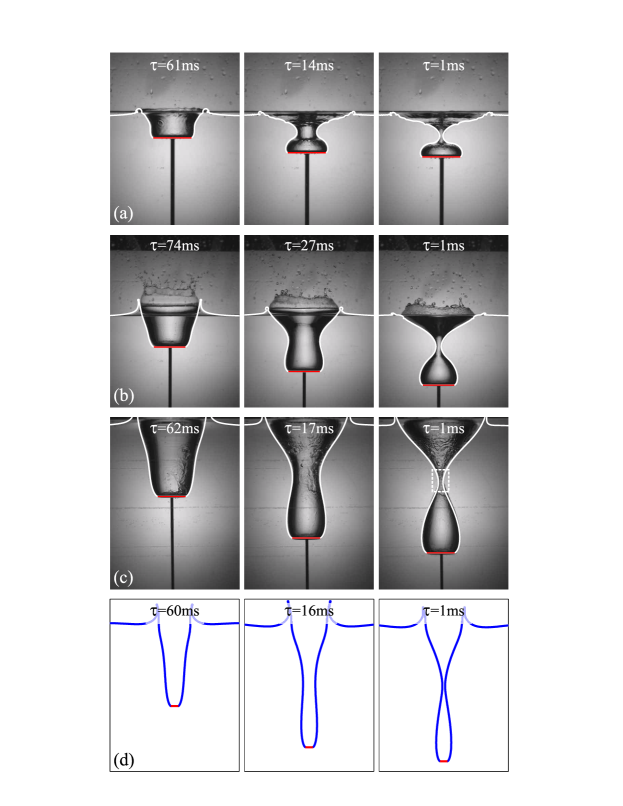
Figure 2: Snapshots of the formation and collapse of a surface void in the plunger experiment: A linear motor pulls down a disk of radius $h_{0}$ = 30 mm through the water surface at a constant velocity (a) $V=0.5$ m/s (Fr = 0.85); (b) $V=1.0$ m/s (Fr = 3.4); (c) $V=2.0$ m/s (Fr = 13.6); and (d) Fr = 200. The collapse of the void is imaged at 1000 frames per second. The lines (overlay) are the void profiles obtained from boundary integral simulations. Without the use of any free parameter, neither in time nor in space, an excellent agreement between the simulation and experiment is found in (a) and (b). Due to a (mild) surface seal there is a discrepancy between the simulations and the experiment in sequence (c), both in the top region near the splash and in the pinch-off region. The region of the dashed box is shown enlarged in Fig. 3. The experimental data for (d) (not shown) is severely dominated by a strong surface seal, which is an air effect and not the focus of the present study.

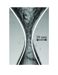
Figure 3: Enlargement of the region around the pinch off point at $\tau=$ 1 ms from the sequence Fig. 2c (Fr = 13.6). A significant discrepancy can be seen for the depth of the pinch–off between the boundary integral simulation (white line) and the experimental recording. The origin of this discrepancy is the airflow in the cavity as will be elaborated elsewhere.

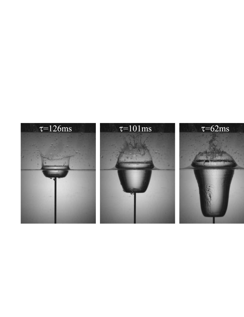
Figure 4: Snapshots of the surface seal which occurs for a disk of radius $h_{0}$ = 30 mm impacting the water surface at a constant velocity of $V=2.0$ m/s (Fr = 13.6), i.e., under the same conditions as Fig. 2c.

The series of events typical for the experimental range of $1<\text{Fr}<100$ is seen in the snapshots of Figs. 2a, b, and c. Upon impact a splash, an outward moving crown of water, is formed. A void is created which collapses due to the hydrostatic pressure and a singularity arises when the collapsing walls of the void collide with each other. Two jets emerge in this experiment: One upwards straight into the air, and one downwards into the entrained air bubble (see Fig. 1b).

In each of Figs. 2a, b, and c the experimental sequence is overlaid with the results of our boundary integral simulation. For Fr=0.85 and Fr=3.4 (Figs. 2a and b), the cavity dynamics is found to be captured extremely well by the numerical result, represented by the overlaid lines. Note that this is a one-to-one comparison between simulation and experiment, without any rescaling in time or space. Due to the axisymmetry of the code it is not possible to capture the full details of the splash and since our focus is on the cavity dynamics we chose to simply take out any droplets which are released from the splash. Surface tension however still expresses itself in small capillary waves in the region of the splash. These waves are most notable in Fig. 2a. As was mentioned before, similar capillary waves (but from a different origin) are found to have a significant influence on the closure of the cavity for a submerging cylinder (Gekle et al. (2008)). For the impacting disk discussed in this paper however they do not affect the closure.

The results for Fr=0.85 in Fig. 2a illustrate the effect of the relative importance of gravity. In the last frame of Fig. 2a it can be seen that the cavity is less symmetric in axial direction around the closure point compared to the experiment performed at Fr=3.4 shown in Fig. 2b. In the third sequence at Fr=13.6 (Fig. 2c), which goes beyond the experimental Froude number range described in Bergmann et al. (2006), significant deviations between the experiment and the numerical cavity shape are found, most notably in the enlargement of Fig. 3 at the depth of the cavity closure. The closure of the cavity is found to be somewhat deeper in the numerics as compared to the experiments. This deviation can be attributed to a secondary effect due to the surrounding air, called the surface seal (see Fig. 4). This phenomenon was first reported by Worthington (1908) and later investigated in more detail by Gilbarg & Anderson (1948). Note that the impact experiment of Fig. 4 is performed under the same conditions as Fig. 2c. The surface seal is the entrainment of the initially outward moving splash by the air rushing into the expanding cavity. If the airflow is strong enough, the splash will close on the axis of symmetry and completely seal off the top of the cavity above the height of the undisturbed water surface.

The surface seal is found to become more pronounced at higher impact velocity, where the surface seal occurs earlier and more liquid is involved in this closure. Accordingly, there is also a larger influence on the shape of the cavity at higher impact velocity. Since this article aims to treat the purely pressure driven collapse of the cavity, without the contributions of the surrounding air, our experimental range is limited by the occurrence of the surface seal. In the simulations we therefore intentionally do not include the air. This explains the discrepancy of Fig. 2c (enlarged in Fig. 3), since contrary to the experiments, no surface seal occurs in the numerics due to the absence of air. In Fig. 2d we go far beyond the experimentally available range by performing simulations at a Froude number of 200.

It is instructive to compare the present boundary integral simulation results with those reported by Gaudet (1998), who reported a bulging contraction of the cavity at the surface level. He found this contraction to close for $\text{Fr}\geq 200$ and interpreted it as a surface seal in the absence of air. We found no evidence for such a surface seal in our simulations, even for considerably larger Froude numbers, and surmise that the effect reported by Gaudet (1998) may be connected to using an insufficient number of nodes in the splash region caused by the limited amount of computational power available at that time.

2.4 Flow field

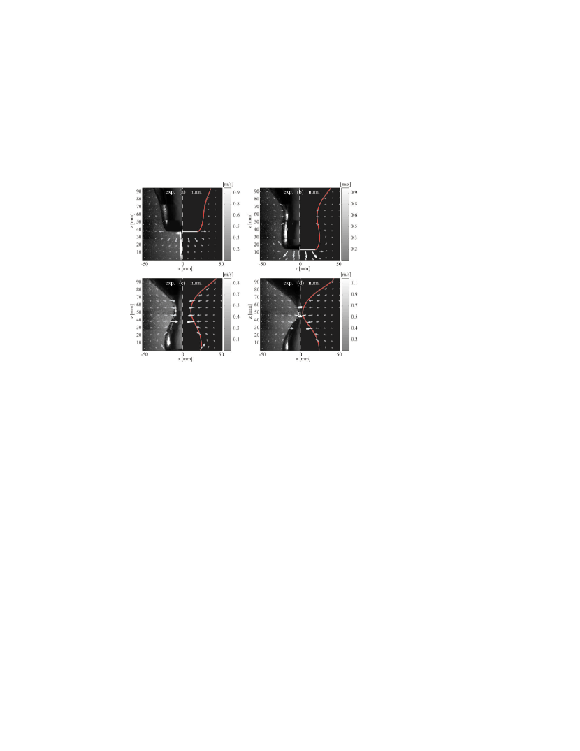
Figure 5: Comparison of the flow field obtained from experiments and boundary integral simulations for a disk of radius $h_{disk}$ = 20 mm which impacts with a velocity of $V=1.0$ m/s (Fr = 5.1). The figures show the flow field at $\tau=$ (a) 49 ms; (b) 25 ms; (c) 7 ms; and (d) 1 ms. The left side of each image shows the flow field (overlaid vectors) obtained from the experiment by four high-speed PIV recordings at 6000 frames per second. The four separate recordings were taken at different depths and combined to give the flow field at high resolution. The recordings on the left side of each image also illustrate the degree of reproducibility of the experiment, as the match between the four PIV recordings at different depths obtained from four repetitions of the same experiment (see main text) is perfect. For clarity only 0.7% of the measured vectors is shown. The right side of each of the images shows the void profile and the corresponding flow field (overlaid vectors) obtained from the boundary integral calculations.

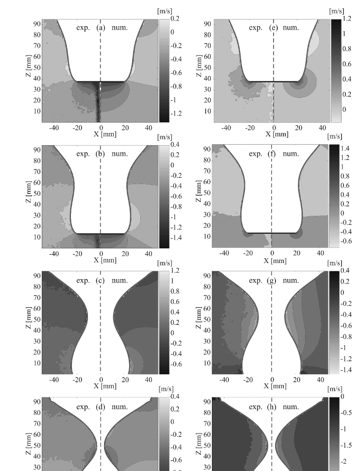
Figure 6: The axial (left figures) and radial (right figures) components of the flow field, representing the same velocity data as in Fig. 5 and taken at the same times $\tau=49$ ms (a,e), 25 ms (b,f), 7 ms (c,g), and 1 ms (d,h). The four images to the left (a-d) compare a contour plot of the axial flow component from the experiment (left side of each image) with that of the numerics (right side of each image). The four images on the right (e-h) show a similar comparison in a contour plot of the radial flow component from the experiment (left side of each image) and numerics (right side of each image). Apart from the region where the rod is pulling down the disk in the experiment, which is absent in the simulation, both components of the flow field show excellent agreement between the experiments and numerical calculations. Again this is a one-to-one comparison of experimental and numerical data without any free parameter, neither in velocity, space, nor time.

In the previous subsection we found the experimental shape of the impact cavity to be well described by our boundary integral simulations if no surface seal occurs. The question we will address in this subsection is whether the simulations also give an accurate description of the surrounding flow field. To this end we will measure the velocity field around the transient cavity through high speed particle image velocimetry (PIV). These experiments are crucial to check the validity of the boundary integral simulations, as the presence of a solid boundary, namely the impacting object, will induce vorticity in the flow. We will compare the experimental flow field to the boundary integral results and finally investigate the radial flow at the depth of closure in more detail.

To perform the PIV measurements, the fluid is seeded with small DANTEC Dynamics polyamid tracer particles of radius $25$ $\mu$m and density $1030$ kg/m³ which follow the flow. A laser sheet shines from the side through the fluid, creating an illuminated plane through the symmetry axis of the cavity. The light scattered by the particles is captured by a high speed camera at a frame rate of 6000 frames per second and a resolution of 1024x512 pixels. The series of recorded images is then correlated by multipass algorithms, using DaVis PIV software by LaVision, in order to determine the flow field in a plane in the liquid. The correlation was performed in two passes at sub-pixel accuracy, using 64$\times$64 pixels and 32$\times$32 pixels interrogation windows. The windows overlap by 50%, resulting in one velocity vector every 16$\times$16 pixels.

In order to obtain high resolution PIV measurements of the flow around the cavity, we made use of the reproducibility of the experiment. The left side of each of the images of Fig. 5 shows the flow around the expanding void by combining the results of four separate PIV measurements at different depths. In this fashion PIV experiments were performed for a field of view of 96 mm $\times$ 56 mm at a spatial resolution of 0.9 mm (In Fig. 5 only 0.7% of the measured vector field is shown). This high resolution makes it possible to simultaneously compare the global flow, as well as the smaller flow structures at the pinch–off depth and the disk’s edge.

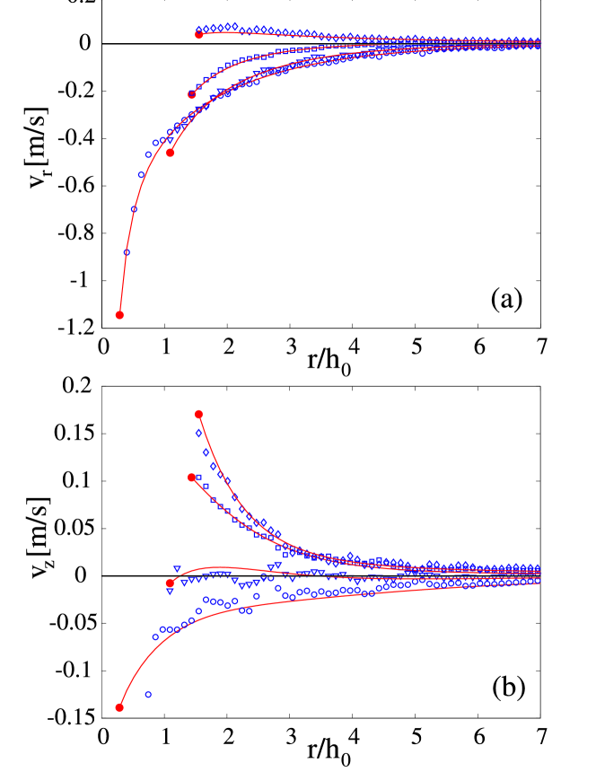
Figure 7: Radial (a) and axial (b) component of the flow at the depth of closure $z_{coll}$ for a disk of radius $h_{disk}$ = 10 mm which impacts at a velocity of $V=1.0$ m/s (Fr = 10.2). The symbols show the result obtained from the PIV measurements at different times, $\lozenge:\tau=$ 30.5 ms; $\square:\tau=$ 20.5 ms; $\triangledown:\tau=$ 10.5 ms; and $\circ:\tau=$ 0.5 ms, and the solid red lines are the corresponding numerical results from the BI simulation. Note that these lines end on the cavity surface (solid red dots). The PIV data is an average of 6 subsequent measurements obtained from the high speed PIV recordings at 6000 frames per second. In consequence, the $v_{r}$ and $v_{z}$ velocity components shown here are the average over one millisecond.

The right side of each image of Fig. 5 shows the numerically obtained cavity profile and flow field. At first sight there appears to be a good agreement, but one would like to obtain a more quantitative comparison between experiment and simulation. This is provided in Fig. 6, which shows contour plots of the axial flow component (Fig. 6a-d) and the radial flow component (Fig. 6e-f) obtained from the PIV measurements (at the left side of each image) and boundary integral simulations (at the the right side of each image). From this figure it is clear that the magnitude as well as the topology of the flow are in excellent agreement. Figures 5 and 6 are a one–to–one comparison between simulation and experiment, and we stress once more, without the use of any free parameter.

In addition to the above, the experimental pictures of Fig. 6 reveal that our initial assumption to neglect the influence of the rod on the flow (see Section 2) is correct. The rod itself is clearly visible in the experimental snapshot of Fig. 5a and the PIV software has correctly detected its downward movement, as can be seen in Figs. 6a–b. From the same figures we also conclude that outside a thin region around the rod the flow remains unchanged. Most importantly, the outward flow at the edges of the disk in Fig. 6e, which is responsible for the expansion of the void, is unaffected by the presence of the rod. This can be understood from the fact that below the disk the radial flow component decays quickly towards the center of the disk whereas the vertical component in the center is equal to the disk speed. As the fluid in the central region hardly moves with respect to the disk, the presence of the rod has a negligible effect on the flow field. We conclude that the boundary layer of the rod makes no contribution whatsoever to the flow field around the cavity.

In Fig. 7 the experimental flow at the closure depth is compared with numerics up to 7 disk radii in radial direction in order to obtain a more quantitative measure of the magnitude of the deviations between the numerical and experimental flow field. We find this deviation to be typically of the order of 0.01 m/s, but it can be slightly larger if the flow velocity is small. This larger inaccuracy at low flow velocities is generic to the PIV method and can most clearly be seen to occur for $\tau=10.5$ ms in Fig. 7b. Overall, a very good agreement is found between the far field flow in the numerics and experiments.

Both in the experiment and simulation we observe that during the expansion of the void the magnitude of the outward radial flow falls off with the distance to the symmetry axis (Fig. 7a). However, once the cavity starts to collapse inward there will be a region around the cavity where the (radial) direction of the flow is reversed and there will be an axisymmetric curved plane (manifold) where the radial flow component vanishes. Here this happens between $\tau=30.5$ ms and $\tau=20.5$ ms (cf. Fig. 7a). In subsection 3.2 we will discuss in detail how this reversal of the radial flow expresses itself in the radial dynamics of the cavity.

3 Modeling the cavity dynamics

In this section we will first derive a simple analytical model for the radial dynamics of the transient cavity. Secondly, we will investigate the surrounding flow, which enters the model through two of the free parameters and causes an asymmetry of the collapse. In the last part of this section we compare the model to the radial dynamics of the cavity observed in experiment and simulation.

3.1 A model for the radial cavity dynamics

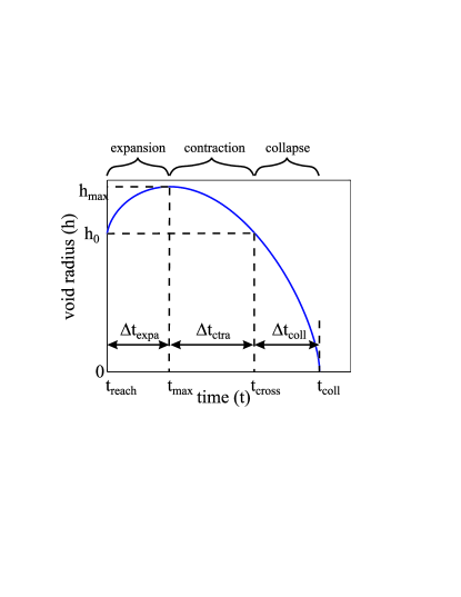
Figure 8: Schematic representation of the three stages in the radial dynamics of the cavity at a constant depth $z$. The first two stages (corresponding to the time interval $\Delta t_{expa}+\Delta t_{ctra}$) are governed by a forcing of the flow by hydrostatic pressure. We can distinguish an expansion and a contraction phase for which the model parameter $h_{\infty}$ differs considerably. In the third stage (corresponding to $\Delta t_{coll}$) the collapsing void accelerates towards the singularity (pinch-off) in which inertia takes over as the driving factor.

The full analytical modeling of a cylindrical symmetric collapse of the transient cavity presents the difficulty of a coupling between the free surface and the flow surrounding the cavity. To tackle this difficulty we propose the convenient simplification of dividing the problem up into a set of quasi two–dimensional problems. If the axial component of the flow is small compared to the horizontal flow components, we can approximate the flow as to be confined to the horizontal plane. In this way an equation for the collapse of a two–dimensional bubble will suffice to describe the cavity dynamics at an arbitrary depth.

To derive such an equation we will closely follow a derivation given in Oguz & Prosperetti (1993) and Lohse et al. (2004). The argument starts by writing the Euler equation in cylindrical coordinates, thereby neglecting the vertical flow component and its derivatives. This means that we assume the flow to be quasi two-dimensional at any depth along the cavity. The azimuthal components can be ignored due to the axial symmetry, leaving the following equation

$$\frac{\partial v_{r}}{\partial t}+v_{r}\frac{\partial v_{r}}{\partial r}=-\frac{1}{\rho}\frac{\partial p}{\partial r}\,,$$ (1)

where $\rho$ denotes the density of the liquid. Under the above assumption of negligible $v_{z}$ and thus $\partial v_{z}/\partial z$, the continuity equation and the boundary conditions on the surface of the void lead to a second equation

$$rv_{r}(r,t)=h(t)\dot{h}(t)\,.$$ (2)

Here, $h(t)$ is the radius of the cavity and its derivative $\dot{h}(t)$ the velocity of the cavity wall at any depth $z$ below the surface. Substituting Eq. (2) into Eq. (1) gives

$$\frac{\partial}{\partial t}\left(\frac{h\dot{h}}{r}\right)+\frac{\partial}{\partial r}\left(\frac{1}{2}v_{r}^{2}+\frac{p}{\rho}\right)=0.$$ (3)

We can integrate this equation over $r$ from the cavity wall $h$ to a reference point $h_{\infty}$, where the flow is taken to be quiescent. This integration yields a Rayleigh-like equation for the void radius at a fixed depth $z$,

$$\Bigg{[}\frac{d(h\dot{h})}{dt}\Bigg{]}\log{h\over h_{\infty}}+{1\over 2}{\dot{h}}^{2}=gz\,.$$ (4)

Here, we have used the fact that the pressure ($p_{\infty}$) driving the collapse of the cavity is provided by the hydrostatic pressure $\rho gz$, where $z$ denotes the depth below the fluid surface. Close to the collapse, the quantity $h_{\infty}$ can be interpreted as the length scale related to the matching of an inner and outer flow region. In the (inner) region near the neck the induced flow looks like a collapsing cylinder as described by Eq. (4), whereas in the (outer) region far from the neck, the flow resembles that of a dipole (plus its image in the free surface). A complete description of the flow would require the matching of these two regions, where $h_{\infty}$ would be determined in the process as the cross–over length scale. $h_{\infty}$ would thus be expected to be of the order of a typical length scale of the process, such as the distance of the cavity surface to the plane where the radial flow vanishes (see Fig. 7a). Therefore, strictly speaking, $h_{\infty}$ is a function of the Froude number and time. In the model presented below we follow a different, simplified route and set $h_{\infty}$ to a constant value (a time averaged value of its dynamics).

We will now use Eq. (4) to analyze the radial dynamics from the initial impact of the disk $t_{0}$ to the time of closure of the cavity $t_{coll}$ at arbitrary depth $z$. In order to obtain an analytical approximate solution, we decompose the cavity dynamics into three different stages, depicted schematically in Figure 8. In this figure the time intervals corresponding to the different stages are denoted as $\Delta t_{expa}$, $\Delta t_{ctra}$, and $\Delta t_{coll}$ respectively. In the first two stages, during $\Delta t_{expa}$ and $\Delta t_{ctra}$, the dynamics is dominated by the hydrostatic pressure forcing. In these stages we observe that the water is first pushed aside by the passing disk, creating an expanding void. At the maximum radius $h_{max}$, the expansion is halted and the void starts to contract. $h_{max}$ is typically of the order of $h_{0}$, e.g., for Fr = 3.4 and Fr = 200 we find respectively $h_{max}\approx 1.3h_{0}$ and $h_{max}\approx 2.4h_{0}$. Since $\dot{h}(t_{max})=0$, we can assume that $\dot{h}(t)$ is small during this expansion and contraction and we can neglect the second term in Eq. (4) leading to

$$\Bigg{[}\frac{d(h\dot{h})}{dt}\Bigg{]}\log{h\over h_{\infty}}=gz\,.$$ (5)

Since $\log(h/h_{\infty})$ varies very slowly in the first regimes, we equate $\log(h/h_{\infty})\approx\log(h(t_{max})/h_{\infty})$ and we solve Eq. (5) using $h(t_{max})=h_{max}$ and $\dot{h}(t_{max})=0$, leading to a parabolic approximation for $h^{2}$,

$$h^{2}(z,t)=h^{2}_{max}-\frac{gz}{\beta}(t-t_{max})^{2}\,,$$ (6)

with $\beta\equiv-\log(h_{max}/h_{\infty}$). The above equation holds for both the expansion stage, the time it takes for the void to grow from $h_{0}$ to $h_{max}$, and the contraction stage, the time it takes to shrink back to $h_{0}$.

In the third stage, during $\Delta t_{coll}$, the collapsing void accelerates towards the singularity and inertia takes over as the dominant factor driving the dynamics of the cavity. This stage can be described using a different approximation to Eq. (4). Near the collapse, $h$ approaches zero, $h_{\infty}$ is typically very large and thus the logarithm diverges. The only way Eq. (4) can remain valid is when the prefactor of the logarithm vanishes. This means that

$$\frac{d(h\dot{h})}{dt}=\frac{1}{2}\frac{d^{2}\left(h^{2}\right)}{dt^{2}}=0\,.$$ (7)

Integration gives the power law of the two-dimensional Rayleigh collapse (cf. Bergmann et al. (2006))

$$h(t)=\sqrt{C}(t_{coll}-t)^{1/2}\,.$$ (8)

In subsection 3.3 the integration constant $\sqrt{C}$ will be determined from continuity of $h$ and $\dot{h}$.

3.2 The influence of the flow on $h_{\infty}$

As an intermezzo in the exposition of the model we now turn to an important point, namely that there is a significantly different quality to the flow in the expansion and the contraction stage. This difference already became clear in our discussion of Figure 7 where we found that in the expansion phase the outward radial flow simply decays with the radial distance, whereas in the contraction phase the radial flow becomes zero at some finite distance at which it changes direction. This is due to the fact that the fluid flows outward until the cavity reaches its maximum radius $h_{max}$, from where it will start to move inward, creating a reversed-flow region around the cavity wall which grows in time. Although in both stages hydrostatic pressure is the dominant factor driving the dynamics of the cavity, there is this dissimilarity in the surrounding flow which needs to be incorporated into the model. To investigate the dynamics of this dissimilarity in detail, we turn to the simulations from which we can obtain the flow field with an arbitrarily fine resolution.

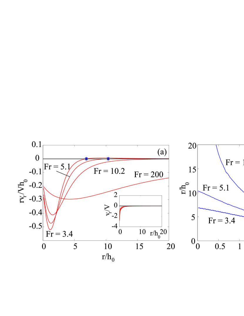
Figure 9: (a) The radial velocity component $v_{r}$ at the moment and depth of closure multiplied by the radial distance $r$ as a function of the same radial distance for different Froude numbers. The inset shows the original radial velocity data. The distance where the radial velocity is zero and the flow is stagnant in radial direction is indicated by the blue stars. The flow can be seen to resemble a radial sink flow more with increasing Froude number as the minimum of $v_{r}r$ decreases with increasing Froude number.
(b) The distance of the point where the radial flow reverses sign to the symmetry axis, determined at the depth of closure as a function of the normalized time remaining till closure $\tau=t_{coll}-t$. Below the curves the flow is directed inwards, above them it is directed outwards. The radial distances of the flow reversal point at $\tau=0$ in this figure correspond to the blue stars of figure (a). The distance of the point of flow reversal is related to the length scales $h_{\infty}^{ctra}$ and $h_{\infty}^{expa}$, which are therefore expected to behave similarly in time.

Figure 9a shows the radial flow component $v_{r}$ multiplied by the radial distance $r$ to the axis of symmetry at the depth and moment of pinch-off. Since the flow at the neck resembles locally a two dimensional sink, whose strength falls off with $1/r$, multiplying $v_{r}$ with $r$ eliminates this geometrical contribution to the flow. For the lower Froude numbers of 3.4 and 5.1 the radial flow component reverses direction at closure depth and time at some distance $r$ (blue stars). At the higher Froude numbers (10.2 and 200) no such point is observed within the numerical domain, which extends to 100 disk radii in the radial direction. This does not mean that such a flow reversal point is absent during the complete time of the collapse, as can be seen in Fig. 9b where we plot the location of the flow reversal point as a function of time: The radial flow reversal point comes into existence at the wall of the void at the moment that the expanded cavity starts to collapse and the flow direction is reversed inward. From then onwards, this point travels away from the axis of symmetry as the collapse is approached ($\tau\rightarrow 0$). In the same figure we also observe that for a higher Froude number the radial flow reversal point travels outward much faster during the cavity collapse as compared to the low Fr case.

The reversed-flow region can be characterized by a stagnation point (or saddle point) in the ($r$,$z$)-plane, corresponding to a circle in three dimensions, where both the axial and the radial velocity components change sign. In Fig. 10 the path of this stagnation point is shown for Fr = 3.4 (a) and Fr = 10.2 (b). For both simulations the stagnation point not only moves away from the axis of symmetry as the pinch-off is approached, but it is also seen to move down in the axial direction and at some point even to cross the depth of closure. A similar path of the stagnation point is observed for all the simulations of Fig. 9 and only at one instant during the collapse of the cavity does the radial flow reversal point at closure depth truly coincide with the stagnation point.

The above leads us to three observations which are relevant for our model of the cavity collapse: (i) Since radial flow reversal at closure depth occurs when the cavity starts to collapse, the topology of the flow differs between the expansion and contraction stage. Since $h_{\infty}$ is the radial distance at which the flow can be assumed to be quiescent ($\mathbf{v}=0$ and $p=p_{\infty}=\rho gz$) it is related to the structure of the surrounding flow, and it is therefore justified to assume different values of $h_{\infty}$ in the respective stages. We will take $h_{\infty}\equiv h_{\infty}^{expa}$ in the expansion stage and $h_{\infty}\equiv h_{\infty}^{ctra}$ in the contraction stage of the model. Just like $h_{\infty}$ in subsection 3.1, $h_{\infty}^{expa}$ and $h_{\infty}^{ctra}$ are set to a constant value, representing the time averaged behavior of $h_{\infty}$ in each respective stage. (ii) As the distance of the radial flow reversal during the contraction moves away faster at higher Froude number, presumably a higher value for $h_{\infty}^{ctra}$ needs to be taken for larger Froude numbers. (iii) In Bergmann et al. (2006) we found that there are two scaling regimes for the neck radius, a first regime where the neck radius scales as a pure power law of time (as in Eq. 8), and a second regime, where a logarithmic correction of time has to be taken into account. The crossover between both regimes is given by the length scale $h_{max}^{2}/h_{\infty}^{ctra}$. As we find from Fig. 9b, for all Froude numbers the distance of the radial flow reversal increases as the pinch-off is approached. Although in theory we assume $h_{\infty}^{ctra}$ to be constant, in reality $h_{\infty}^{ctra}$ thus increases as the pinch–off is approached. This means the cross–over length scale $h_{max}^{2}/h_{\infty}^{ctra}$ decreases with time.
Therefore the time needed for the collapsing neck to decrease to $h_{max}^{2}/h_{\infty}^{ctra}$ will be longer as compared to the assumption of a constant (initial) value for $h_{\infty}^{ctra}$ and may even never reach this second regime. The effect is stronger for increasing Froude number, since the radial flow reversal point at closure depth moves away faster and further at higher Froude number.

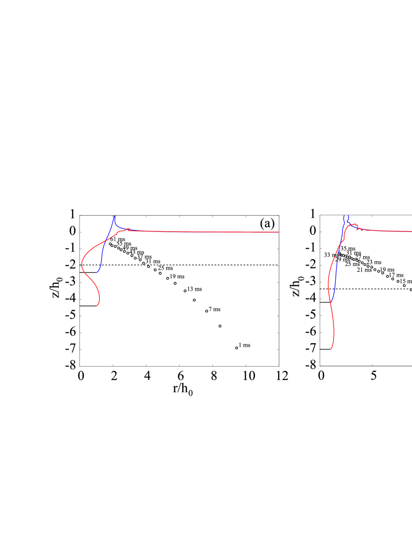
Figure 10: The open circles show the path of the stagnation point of the flow for Froude 3.4 (a) and 10.2 (b). For (a) the first observation of the stagnation point is made at $\tau=61$ ms until 1 ms before closure at intervals of 3 ms. In (b) the first observation is made at $\tau=35$ ms until 7 ms before closure at intervals of 1 ms. For clarity the time till closure is indicated only for every second observation. Further more, the void profiles at the time of the first (blue) and last (red) observation are shown. The depth of closure is indicated by the dotted line.

3.3 The free parameters of the model

In this subsection we continue our derivation of a simplified model for the radial cavity dynamics started in subsection 3.1. As argued in the previous subsection it is justified to assume different (constant) values for $h_{\infty}$ during the expansion and contraction stage of the void. We therefore introduce different values for $\beta$ in Eq. (6), depending on whether we are in the expansion or in the contraction stage

$$\beta=\Big{\{}\begin{array}[]{cc}\beta_{expa}\equiv-\log(h_{max}(z)/h_{\infty,expa})&t<t_{max}\\ \beta_{ctra}\equiv-\log(h_{max}(z)/h_{\infty,ctra})&t>t_{max}\\ \end{array}\,.$$ (11)

Note that with this definition $\beta_{expa}$ and $\beta_{ctra}$ are positive quantities as for both holds $h_{\infty,expa},h_{\infty,ctra}\gg h_{max}$. Secondly, the fact that $\beta$ depends only logarithmically on $h_{\infty}$ furthermore justifies approximating the time-dependent quantity $h_{\infty}(t)$ by its time-average $h_{\infty}$.

Now, to determine $h_{max}$, or rather the time it will take to get there from the time the disk passes at $t=t_{reach}$, we need the radial velocity of the initial expansion at $t=t_{reach}$ (see Fig. 8). A reasonable assumption (and similar to the proposition of Duclaux et al. (2007)) is that the disk displaces water from underneath itself to the sides at a velocity directly proportional to its downward velocity. Therefore, we have

$$\dot{h}(t_{reach})=\alpha_{expa}V\,.$$ (12)

For the velocity at the end of the contraction phase at $t_{cross}=t_{reach}+\Delta t_{expa}+\Delta t_{ctra}$, we write in a similar fashion

$$\dot{h}(t_{cross})=-\alpha_{ctra}V\,.$$ (13)

Clearly, both $\alpha_{expa}$ and $\alpha_{ctra}$ are again positive quantities.

The analytical model for the radial cavity dynamics given by Eq. (6) and Eq. (8) thus has four unknown parameters $\alpha_{expa}$, $\beta_{expa}$, $\alpha_{ctra}$, and $\beta_{ctra}$. The value of C in Eq. (8) follows from the fact that the trajectory and its derivative in Fig. 8 should be continuous. We assume the collapse regime to start at the end of the contraction phase, where we have $h(t_{cross})=h_{0}$ and $\dot{h}(t_{cross})=-\alpha_{ctra}V$. From these conditions, the value of $C$ is readily obtained,

$$C=2h_{0}\alpha_{ctra}V\,.$$ (14)

However, for given $\alpha_{expa}$, $\beta_{expa}$, and $\beta_{ctra}$, the constant $\alpha_{ctra}$ is also uniquely determined by the continuity of the trajectory and its derivative at $h(t_{max})=h_{max}$ , which gives

$$\alpha_{ctra}=\alpha_{expa}\sqrt{\beta_{expa}/\beta_{ctra}}\,,$$ (15)

and leaves only $\alpha_{expa}$, $\beta_{expa}$, and $\beta_{ctra}$ to be determined.

Summarizing, the time evolution of the cavity at depth $z$ is described by the following three equations

$$h(z,t)= \sqrt{h^{2}_{max}-\frac{gz}{\beta_{expa}}(t-t_{max})^{2}} \qquad\text{for }t_{reach}<t\leq t_{max}\,,$$ (16)

$$h(z,t)= \sqrt{h^{2}_{max}-\frac{gz}{\beta_{ctra}}(t-t_{max})^{2}} \qquad\text{for }t_{max}<t\leq t_{cross}\,,$$ (17)

$$h(z,t)= \sqrt{2h_{0}\alpha_{ctra}V}\sqrt{t_{coll}-t} \qquad\text{for }t_{cross}<t\leq t_{coll}\,,$$ (18)

where the times $t_{reach}$, $t_{max}$, $t_{cross}$, and $t_{coll}$ are readily related to the impact time $t=0$ (which will be done explicitly in section 4) and $h_{max}$ is given by

$$h_{max}(z)=h_{0}\sqrt{1+\alpha_{expa}^{2}\beta_{expa}\frac{V^{2}}{gz}}\,,$$ (19)

as can be easily derived, e.g., from Eq. 16 together with its boundary conditions $h(z,t_{reach})=h_{0}$ and $\dot{h}(z,t_{reach})=\alpha_{expa}V$.

3.4 Validation of the model

We will now compare the dynamics of the radius of the void at closure depth with the theoretical prediction of Eq. (6) and Eq. (8) to validate the model and quantify the influence of the flow reversal on $\beta_{expa}$ and $\beta_{ctra}$.

The parameter $\alpha_{ctra}$ is eliminated by the relation Eq. (15), leaving three parameters to match Eqs. (16)–(18) to the radial dynamics from the boundary integral simulations. At first sight, one could assume that the initial outward velocity $\alpha_{expa}V$ could be easily obtained from simulation or experiment, since it is observed as the angle at which the free surface leaves the disk. However, when this angle is investigated in closer detail, it is found to strongly depend on the distance from the disk’s edge over which it is measured. In the numerics, close enough to the disk’s edge, the free surface even becomes nearly parallel with the disk. This means that although $\alpha_{expa}V$ is useful as a (theoretical) concept, it is not directly measurable and should therefore be determined by a fitting routine.

The three parameters $\alpha_{expa}$, $\beta_{expa}$, and $\beta_{ctra}$ are determined by a least square fit to the radial dynamics of the cavity at closure depth obtained from the simulations. Fig. 11a shows the comparison between these fits of Eqs. (16)–(18) (red dashed line) and the simulations (blue solid line) at two different Froude numbers of 3.4 and 200. The approximation is found to be in excellent agreement throughout the collapse, faithfully reproducing the maximum expansion of the cavity and the complete time of collapse.

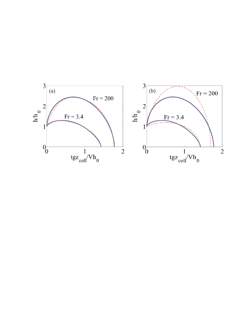
Figure 11: (a) The time evolution of the radius of the cavity at closure depth for different Froude numbers. The solid blue lines represent the simulation results and the dashed red lines correspond to a least square fit of the approximation given by Eqs. (16)-(18). (b) The same numerical time evolution data as in (a) (solid blue lines) are now approximated by the model proposed by Duclaux et al. (2007), which consists of Eqs. (16)–(17) with $\beta_{expa}$ and $\beta_{ctra}$ set to 1, again from a least squares fit (dashed red lines). In both (a) and (b) time has been rescaled by a factor $Vh_{0}/gz_{coll}$ in order to show the results for the two Froude numbers in a single plot.

In Figure 12a we find the parameters $\alpha_{expa}$, $\beta_{expa}$, and $\beta_{ctra}$ as a function of the Froude number, determined by repeating the fitting routine described above for many impact velocities. All are found to weakly depend on the Froude number (note that a logarithmic scale has been used for Fr). For completeness we also plot the derived quantity $\alpha_{ctra}$, calculated from Eq. 15.

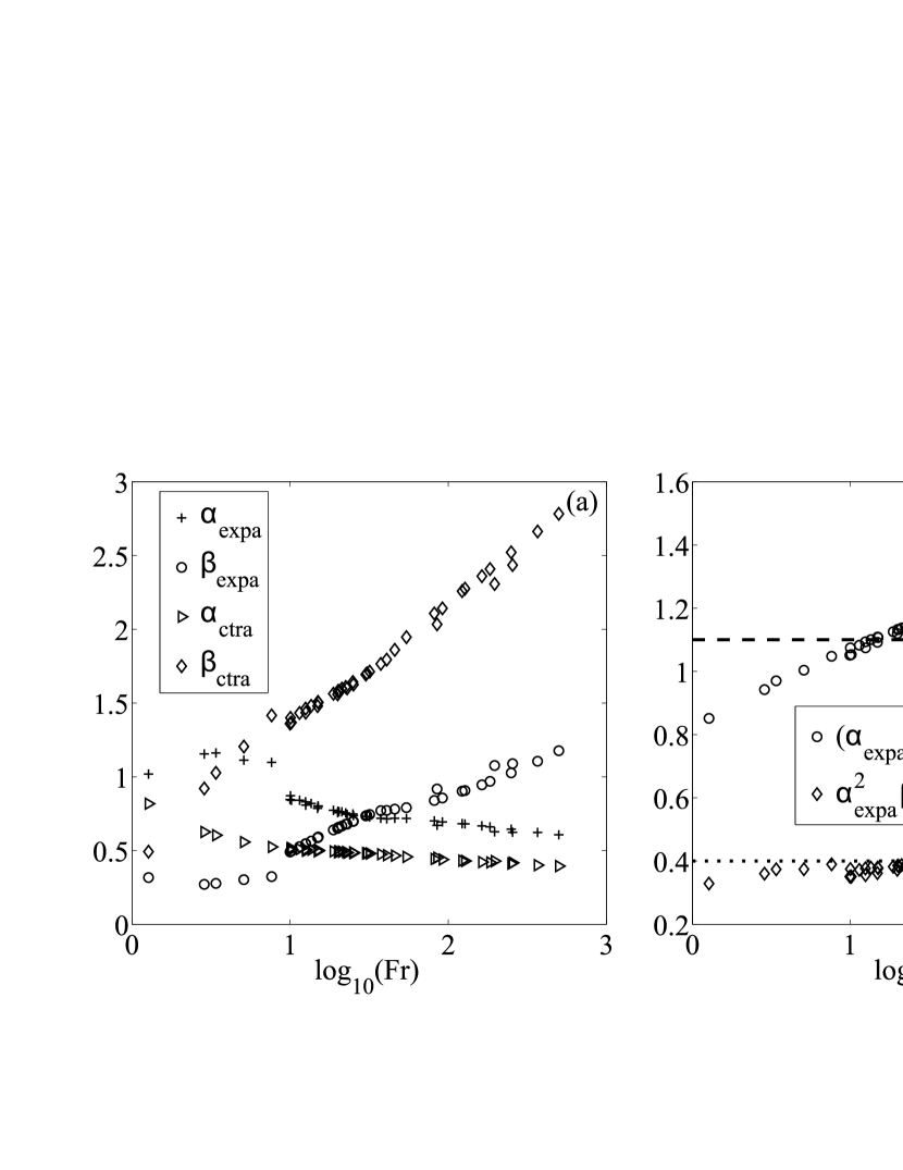
Figure 12: (a) The parameters $\alpha_{expa}$, $\beta_{expa}$, $\alpha_{ctra}$, and $\beta_{ctra}$ obtained from the fitting routine used in Fig. 11a. All are found to weakly depend on the Froude number (note the logarithmic scale for Fr). (b) The quantities $\sqrt{\alpha_{expa}\beta_{expa}+\alpha_{ctra}\beta_{ctra}}$ and $\alpha_{expa}^{2}\beta_{expa}$ calculated from (a). Whereas $\sqrt{\alpha_{expa}\beta_{expa}+\alpha_{ctra}\beta_{ctra}}$ is found to weakly depend on the Froude number, $\alpha_{expa}^{2}\beta_{expa}$ has a nearly constant value of 0.40. (horizontal dotted line). In comparison with $\sqrt{\alpha_{expa}\beta_{expa}+\alpha_{ctra}\beta_{ctra}}$, the horizontal dashed line indicates the value $C_{1}=1.10$ obtained from a best fit to the closure depth data of Fig. 13.

If in Eqs. (16)–(17) the constants $\beta_{expa}$ and $\beta_{ctra}$ are set to 1 and therefore by Eq. (15), $\alpha_{ctra}=\alpha_{expa}$, we arrive at the cavity dynamics proposed by Duclaux et al. (2007) for impacting spheres and cylinders. These dynamics are shown in Fig. 11b with the only free parameter $\alpha_{expa}$ also determined by a least square fit to the data. This approximation is seen to qualitatively reproduce the trend for the maximum expansion and collapse time, but fails to capture the exact values. It is also conceptually different, as Duclaux et al. (2007) propose the cavity dynamics to be symmetric around the maximum expansion, while our model captures the asymmetry around this point in time that is also found in experiment and simulation. Our solution Eqs. (16)–(17) is explicitly not symmetric, since it allows for different values of $\beta$ at $t<t_{max}$ and $t>t_{max}$.

To conclude this section we return to the first two observations we made at the end of subsection 3.2 on the motion of the stagnation point and the plausible consequences for $h_{\infty}$. (i) The flow reversal which occurs when the cavity starts to collapse indeed introduces an asymmetry in the behavior around the maximum expansion. This is clearly observed in the radial dynamics of Fig. 11, especially for $\text{Fr}=3.4$. (ii) As the distance of the radial flow reversal during the collapse moves away faster at higher Froude number (see Fig. 9b), we indeed have to introduce a larger $h_{\infty}^{ctra}$ (corresponding to a larger $\beta_{ctra}$) for higher Froude number in the fit of Fig. 11a to account for this effect.

4 Characteristics of the Transient Cavity

Now that we derived a simplified model for the radial dynamics of the cavity, we will use it, together with the simulations and experiments, to investigate the following key characteristics of the transient cavity: (i) the depth of the pinch-off and the depth of the disk at the moment of pinch–off (subsection 4.1), and (ii) the amount of air entrained through the cavity collapse (subsection 4.2). Besides this we elaborate on our previous findings from Bergmann et al. (2006) in the Appendix A. There we revisit the dynamics of the cavity at closure depth (Appendix A.1) and the cavity shape around the minimal radius (Appendix A.2). Finally, in Appendix B we discuss the time evolution of the vertical position of the minimal cavity radius and place it within the context of the model.

4.1 Closure depth

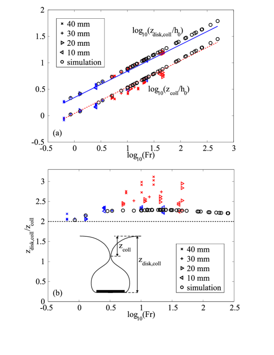
Figure 13: (a) Double logarithmic plot of the depth at which the void collapses $z_{coll}$ and the depth $z_{disk,\,coll}$ of the disk at collapse time for experiments with four different disk radii (see legend) and for the boundary integral simulations (open circles), all as a function of the Froude number. Experiments in which a surface seal occurs during the collapse are indicated by red symbols, the experiments without a surface seal by blue symbols. Here, a surface seal is said to occur if at some point in time due to air suction the splash closes onto itself and the cavity is completely sealed off. The experiments without a surface seal are found to agree well with the numerically obtained values (open circles) and the theoretical prediction for the scaling of $z_{coll}/h_{0}=C_{1}Fr^{1/2}$ (red dashed line) and $z_{disk,\,coll}/h_{0}=2C_{1}Fr^{1/2}$ (blue solid line), with $C_{1}=1.10$ obtained from a fit to the data of $z_{coll}$. The experiments for which a surface seal occurs are seen to slightly deviate from this prediction.
(b) The ratio of the depth of the disk at the time of pinch-off $z_{disk,\,coll}$ and the pinch-off depth $z_{coll}$ for different disk radii as a function of the Froude number. The experiments without a surface seal (blue symbols) agree well with the numerical results (open circles). The ratio for the numerical result and experiments without a surface seal lie close to the predicted value of 2 indicated by the black dashed line. The experiments in which a surface seal occurs are again indicated by the red symbols and found to deviate more with increasing Froude number for a fixed disk size. The inset shows the definition of the depths $z_{coll}$ and $z_{disk,coll}$ at the closure time.

Following Glasheen & McMahon (1996), Gaudet (1998), and Duclaux et al. (2007) we will characterize the shape of the cavity at pinch–off by the depth of closure $z_{coll}$, i.e., the depth at which the pinch–off takes place. To capture more information on the full shape of the void, we will also investigate how $z_{coll}$ relates to the total depth of the cavity $z_{disk}(t_{coll})=z_{disk,\,coll}$ at the time of collapse (or closure) (see the inset of Fig. 13).

A comprehensive argument for the scaling of $z_{coll}$ can be obtained by following a similar procedure to the one outlined in Lohse et al. (2004) for the determination of the closure depth after the impact of a steel ball on soft sand. The difference is that whereas in sand one can assume that due to the compressibility of the material there is hardly any outwards motion of the sand, here we are dealing with an incompressible fluid and the outward expansion of the cavity needs to be taken into account.

The time interval between impact of the disk and collapse of the cavity $\Delta t=t_{coll}-t_{0}$ at any depth $z$ consists of two main parts: First, the disk needs an amount of time $\Delta t_{reach}$ to reach the depth $z$. Second, just after the disk passes there is the time $\Delta t_{void}$ it takes for the void to form, expand, and collapse

$$\Delta t=\Delta t_{reach}+\Delta t_{void}\,.$$ (20)

The first term equals $\Delta t_{reach}=z/V$ since the velocity of the disk is constant in the experiment and simulation. In Section 3 $\Delta t_{void}$ was decomposed into three stages as is schematically depicted in Fig. 8. The collapse time can thus be written as,

$$\Delta t=\Delta t_{reach}+\underbrace{\Delta t_{expa}+\Delta t_{ctra}+\Delta t_{coll}}_{\Delta t_{void}}\,.$$ (21)

To estimate these last three timescales at arbitrary depth $z$, we turn to our model for the cavity dynamics Eqs. (16)-(18).

If we combine the conditions Eq. (12) and Eq. (13) with the time derivative of Eqs. (16) and (17), we readily obtain

$$\Delta t_{expa}=\alpha_{expa}\beta_{expa}\frac{h_{0}V}{gz}\,,$$

$$\Delta t_{ctra}=\alpha_{ctra}\beta_{ctra}\frac{h_{0}V}{gz}\,.$$ (22)

Recall that $\alpha_{ctra}=\alpha_{expa}(\beta_{expa}/\beta_{ctra})^{1/2}$. The radial collapse during $\Delta t_{coll}$ is in turn described by the approximation of Eq. (18). Since $h(t_{cross})=h_{0}$ we find for this time interval

$$\Delta t_{coll}=t_{coll}-t_{cross}=\frac{1}{2\alpha_{ctra}}\frac{h_{0}}{V}\,.$$ (24)

Collecting all the above time intervals, within the model the total amount of time that passed from the impact of the disk until the collapse of the cavity at depth $z$ is given by

$$\Delta t = \Delta t_{reach}+\Delta t_{expa}+\Delta t_{ctra}+\Delta t_{coll}$$ (25)

$$= \frac{z}{V}+(\alpha_{expa}\beta_{expa}+\alpha_{ctra}\beta_{ctra})\frac{h_{0}V}{gz}+\frac{1}{2\alpha_{ctra}}\frac{h_{0}}{V}\,.$$

Now, to find the closure depth $z_{coll}$, we need to determine at what depth the collapse will occur first, which we can do by solving

$$\frac{d\Delta t}{dz}=0\,.$$ (26)

This gives

$$\frac{z_{coll}}{h_{0}}=\sqrt{\alpha_{expa}\beta_{expa}+\alpha_{ctra}\beta_{ctra}}\text{Fr}^{1/2}\,.$$ (27)

In addition, the total depth of the disk at the time of collapse, $z_{disk}(t_{coll})=z_{disk,\,coll}$, can be obtained by inserting Eq. (27) into Eq. (25) to give $z_{disk,\,coll}=V\Delta t$, or

$$\frac{z_{disk,\,coll}}{h_{0}}=2\sqrt{\alpha_{expa}\beta_{expa}+\alpha_{ctra}\beta_{ctra}}\text{Fr}^{1/2}+\frac{1}{2\alpha_{ctra}}\,.$$ (28)

When we compare these expressions with the experiments without a surface seal (blue symbols) and the numerical calculations (black circles) in Fig. 13a we find a very good agreement with the prediction of Eq. (27). A fit to the data of $z_{coll}$ gives $z_{coll}/h_{0}=C_{1}\text{Fr}^{1/2}$, with $C_{1}=1.10$. The agreement of the experiments in which a surface seal occurs (red symbols) deteriorates for a fixed disk size with increasing Froude number, since the surface seal becomes more disruptive at higher impact velocities.
In the same figure we find the experimental and numerical results for the total depth of the disk at closure $z_{disk,\,coll}$. From the apparent power-law scaling it is clear that the constant $1/(2\alpha_{ctra})$ in Eq. (28) has no significant contribution. The total depth of the void is found to scale as $z_{disk,\,coll}/h_{0}=C_{2}\text{Fr}^{1/2}$, with $C_{2}=2.49$ close to the expected value of $C_{2}=2C_{1}=2.2$ that follows from Eqs. (27) and (28). The fact that the closure depth and the total depth have the same power-law scaling $\text{Fr}^{1/2}$ indicates that the time from the initial impact of the disk to the time of closure of the cavity does not depend on the velocity of the impact, since $\Delta t=z_{disk,\,coll}/V=C_{2}\sqrt{h_{0}/g}$.

This is in agreement with the findings of Glasheen & McMahon (1996), who experimentally observed a similar scaling for the impact of a disk on a water surface, although with a slightly different prefactor of $C_{2}\approx 2.3$. Duclaux et al. (2007) also found the scaling of $\Delta t$ ($\propto\sqrt{h_{0}/g}$) for impacting spheres and furthermore reported $z_{disk,\,coll}/h_{0}=2z_{coll}/h_{0}\propto\text{Fr}^{1/2}$ in agreement with our observations.

To investigate the data of Fig. 13a more closely it is convenient to take the ratio of $z_{coll}/z_{disk,\,coll}$ (see Fig. 13b). According to Eq. (27) and Eq. (28), this ratio should scale as

$$z_{coll}/z_{disk,\,coll}=2+\frac{1}{2\alpha_{ctra}\sqrt{\alpha_{expa}\beta_{expa}+\alpha_{ctra}\beta_{ctra}}}\text{Fr}^{-1/2}\approx 2\,$$ (29)

in the limit of large Froude number. In Fig. 13b the ratio of $z_{coll}/z_{disk,\,coll}$ in the experiments without a surface seal (blue symbols) and the numerical calculations (black circles) are indeed close to the constant value of 2 (dashed black line), but at lower Froude number it decreases slightly contrary to the proposed scaling by the second term in Eq. (29). Although the second term of the ratio of Eq. (29) should become relevant when the Froude number is considerably small, this is not observed in Fig. 13b. This can be understood by noting that in the limit of small Froude number our assumption of non-interacting fluid layers from Eq. (4) breaks down as gravity becomes more important and thus Eq. (29) is no longer valid. In Fig. 13b it is again illustrated that the experiments with a surface seal (red symbols) deviate more and more from the simulations without air as the Froude number increases.

The fits to the trajectories discussed in subsection 3.4 provide us with the parameters $\alpha_{expa}$, $\beta_{expa}$, and $\beta_{ctra}$ (recall that $\alpha_{ctra}$ is given by Eq. (15)), and therewith with an independent way of determining the proportionality constant $\sqrt{\alpha_{expa}\beta_{expa}+\alpha_{ctra}\beta_{ctra}}$ of Eq. 27. Repeating this fitting procedure for many impact velocities results in Fig. 12b, where $\sqrt{\alpha_{expa}\beta_{expa}+\alpha_{ctra}\beta_{ctra}}$ is plotted as a function of $\log_{10}\text{Fr}$. A weak (logarithmic) dependence on the Froude number is revealed. It can also be seen that the value $C_{1}\approx 1.10$ of the proportionality constant in Eq. (27) found from the fit to the closure depth data in Fig. 13 is consistent with the data when one wants to disregard the Fr dependence.

4.2 Air Entrainment

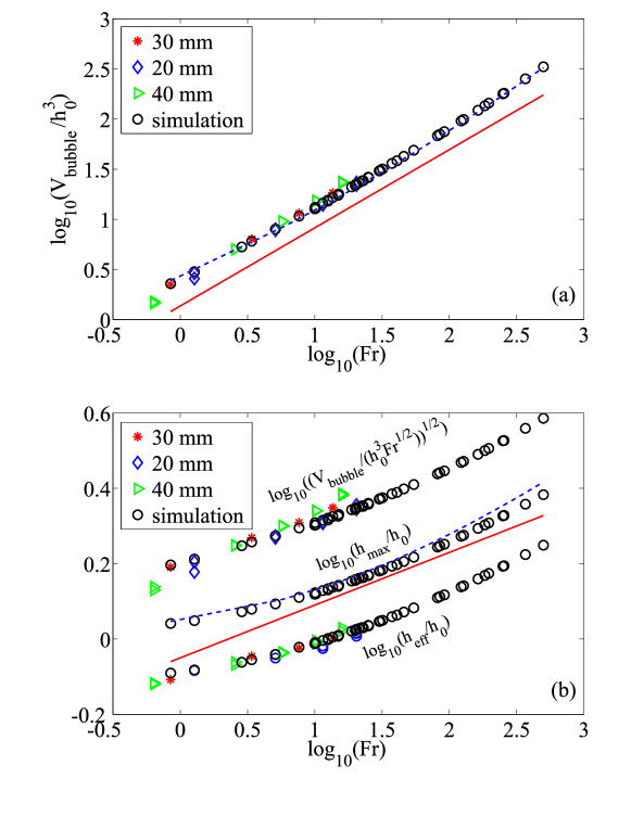
Figure 14: (a) The volume of the bubble $V_{bubble}$ entrained during the collapse of the cavity from experiments (colored symbols) and simulations (black open circles), normalized by the cubed disk radius $h_{0}^{3}$, as a function of the Froude number in a double logarithmic plot. The data suggest a power-law scaling $V_{bubble}/h_{0}^{3}\propto\text{Fr}^{\lambda}$ where a linear best fit through the data between $\text{Fr}=2.5$ and $250$ gives $\lambda\approx 0.78$ (solid red line, shifted for clarity). The dashed blue line corresponds to the model prediction Eq. (32).
(b) Double logarithmic plot of three quantities that measure the radial length scale of the entrapped air bubble. From bottom to top: the effective (or average) radius $h_{\textit{eff}}$ of the bubble at pinch–off (Eq. (33)), the maximum radius of the bubble $h_{max,\,coll}$ at pinch–off, and the square root of the bubble volume compensated for the expected scaling of its vertical extension $[V_{bubble}/h_{0}\text{Fr}^{1/2}]^{1/2}$, all compensated with the disk radius $h_{0}$. The dashed blue line is the model prediction Eq. (31) and the solid red line represents a power law with the scaling exponent $\lambda=0.14$ expected from Eq. (30).

After pinch-off, an air bubble is entrapped, as is clearly visible in Figs. 1b and 2. The (rescaled) volume of this bubble $V_{bubble}/h_{0}^{3}$ is not only found to solely depend on the Froude number, but also to exhibit close to power-law scaling behavior: The scaling law for the volume of the bubble observed in experiment and simulation is found to be $V_{bubble}/h_{0}^{3}\propto\text{Fr}^{\lambda}$, with $\lambda=$ 0.78 (see Fig. 14a).
This is surprising, since for the impact of a liquid mass on a free surface the volume of air entrained in the process scales with a different exponent $V_{bubble}\propto\text{Fr}^{1.0}$ (Prosperetti & Oguz (1997)). In this section we will try to shed light onto the origin of this scaling behavior using our findings of Section 4.1.

In Section 4.1 it was found that the axial length of the enclosed bubble at pinch–off scales roughly as $(z_{coll}-z_{disk,\,coll})/h_{0}\approx 1.10\,\text{Fr}^{1/2}$, if we ignore the weak Froude number dependence of the prefactor $\sqrt{\alpha_{expa}\beta_{expa}+\alpha_{ctra}\beta_{ctra}}$ (see Fig. 12b). Therefore, the scaling of the axial length $z_{coll}-z_{disk,\,coll}$ of the enclosed bubble cannot by itself account for the observed scaling of $V_{bubble}$. The radial length scale $h_{rad}$ of the bubble must therefore be Froude number dependent and should scale as

$$\frac{h_{rad}}{h_{0}}\propto\left[\frac{V_{bubble}}{h_{0}^{2}(z_{disk,coll}-z_{coll})}\right]^{1/2}\propto\left[\frac{\text{Fr}^{0.78}}{\text{Fr}^{0.50}}\right]^{1/2}=\text{Fr}^{0.14}\,.$$ (30)

Now what would we expect based on our simplified model? The maximum radial expansion of the cavity at any depth $z$ is given by $h_{max}(z)$, see Eq. (19). As the depth $z_{max}$ at which the radial size of the bubble is maximal is somewhere between the closure depth $z_{coll}$ and the depth of the disk at closure $z_{disk,\,coll}$, we have $z_{max}\approx(z_{coll}+z_{disk,\,coll})/2=(3/2)\sqrt{\alpha_{expa}\beta_{expa}+\alpha_{ctra}\beta_{ctra}}\text{Fr}^{1/2}$. If we insert this depth into $h_{max}(z)$, Eq. (19), we find

$$h_{rad} \propto h_{max}(z_{max})\approx h_{0}\sqrt{1+\frac{2\alpha_{expa}^{2}\beta_{expa}}{3\sqrt{\alpha_{expa}\beta_{expa}+\alpha_{ctra}\beta_{ctra}}}\text{Fr}^{1/2}}$$ (31)

$$\approx h_{0}\sqrt{1+0.26\,\text{Fr}^{1/2}}\,.$$

In the last (approximate) equation we have used that $\sqrt{\alpha_{expa}\beta_{expa}+\alpha_{ctra}\beta_{ctra}}\approx 1.10$ and $\alpha_{expa}^{2}\beta_{expa}\approx 0.40$ (cf. Fig. 12b). If a power-law fit $h_{rad}/h_{0}$ vs. Fr is enforced on this dependence in the regime $2.5<\text{Fr}<250$ one obtains the observed effective exponent $0.14$, $h_{rad}/h_{0}\propto\text{Fr}^{0.14}$. Alternatively, by taking the square of Eq. (31) and multiplying with the vertical extension $(z_{coll}-z_{disk,\,coll})$ of the bubble we find the following prediction for the bubble volume

$$V_{bubble}\propto h_{0}^{3}\left(1+0.26\,\text{Fr}^{1/2}\right)\text{Fr}^{1/2}\,.$$ (32)

Clearly, the model predicts power-law scaling only in the limit of large Froude numbers. Moreover, as in this limit $V_{bubble}\propto\text{Fr}$, the scaling prediction is in agreement with the Prosperetti & Oguz (1997) result. Again, in the regime $2.5<\text{Fr}<250$ the effective exponent is $0.78$.

We test the above prediction by looking at three different quantities that capture the radial expansion of the cavity in experiment and numerics. The first is the effective, or average, radius $h_{\textit{eff}}$ of the bubble which is computed directly from the experimental and numerical cavity profiles (i.e., without any scaling assumption of the axial length scale) at the pinch-off time by

$$h_{\textit{eff}}^{2}=\frac{1}{\left(z_{disk,\,coll}-z_{coll}\right)}\int_{z_{disk,\,coll}}^{z_{coll}}h^{2}(z)dz\,.$$ (33)

The second quantity we look at is the maximal radius of the bubble $h_{max,\,coll}$ at the time of pinch–off which is a more direct measure of the expansion of the cavity. $h_{max,\,coll}$ can be directly observed from the cavity profile at the time of pinch–off as the maximal radius for a depth between $z_{disk,\,coll}$ and $z_{coll}$.

In Figure 14b we compare these two quantities $h_{\textit{eff}}/h_{0}$ and $h_{max,\,coll}/h_{0}$ with a third, namely the measured $V_{bubble}$ compensated for the expected scaling behavior of its axial extension $z_{disk,coll}-z_{coll}\propto h_{0}\text{Fr}^{1/2}$, i.e., $V_{bubble}/h_{0}^{3}\text{Fr}^{1/2}$. All of these three quantities follow the same trend, which is well described by the prediction Eq. (31) from the model (the blue dashed line in Fig. 14b), and close to the expected $\text{Fr}^{0.14}$ scaling which is indicated by the solid red line. Finally, comparing the measured bubble volume $V_{bubble}/h_{0}^{3}$ with the model prediction Eq. (32) in Fig. 14a (dashed blue line), we find excellent agreement.

5 Conclusions

In this article we investigate the purely gravitationally induced collapse of a surface cavity created by the controlled impact of a disk on a water surface. We find excellent agreement between experiments and boundary integral simulations for the dynamics of the interface, as well as for the flow surrounding the cavity. The topology and the magnitude of the flow in the simulations agree perfectly with the PIV results.
In experiments it is found that a secondary air effect, the “surface seal”, has a significant influence on the cavity shape at high Froude number. Since the surface seal phenomenon (and its influence) is more pronounced at higher impact velocities, it limits our experimental Froude number range. In the boundary integral simulations the air was intentionally excluded, thus avoiding this limitation.

Because the velocity of the impacting disk is a constant control parameter in our experiments, a simple theoretical argument based on the collapse of an infinite, hollow cylinder describes the key aspects of the transient cavity shape.

This model accurately reproduces the dynamics of the cavity including its maximal expansion and total collapse time. It also captures the scaling for the depth of closure and the total depth of the cavity at pinch–off, and predicts their ratio to be close to 2, where 2.1 is found in experiments and simulation.
There is a close similarity of this description to the cavity dynamics proposed by Duclaux et al. (2007). However, by introducing the asymmetry between the radial expansion and collapse, we find a better agreement between the theory and the radial dynamics of the cavity. The fact that the flow is qualitatively different during expansion of the cavity on the one hand and its contraction on the other is found to be responsible for the asymmetry. Our approach is also conceptually different, as Duclaux et al. (2007) take $\alpha_{expa}$ to be independent of the Froude number, while we allow it to be weakly dependent on Froude and, more importantly, our description includes the last stage of the collapse, which is solely driven by inertia.

We find the volume of air entrained by the impact of the disk to behave as $V_{bubble}/h_{0}^{3}\propto(1+0.26\text{Fr}^{1/2})\text{Fr}^{1/2}$. This dependence is set by the Froude dependence of two length scales, namely the axial length scale, distance between the pinch-off point and the disk, and the radial expansion of the cavity. Here we have excellent agreement between the experimental and numerical findings and the prediction of the model.

Finally, the appendices deal with the time evolution of the cavity radius we discussed previously in Bergmann et al. (2006). In this paper, and subsequent papers dealing with the universality of the last stages of the pinch-off from a theoretical point of view (Gordillo & Pérez-Saborid (2006) and Eggers et al. (2007)), the pinch-off is assumed to be symmetric around the closure depth, whereas in experiment and numerics we observe that the minimal radius of the void actually moves downward in time. As this (small) axial translation could be relevant for this universality issue, it is studied in detail in Appendix B, where we find that it can be included within the model presented in this paper, as a secondary effect.

Appendix A Revisiting Bergmann et al. (2006)

In this appendix we will review the results which were presented in Bergmann et al. (2006) as far as they are necessary for the understanding of the material in Appendix B, together with some additional results.

A.1 Neck radius at closure depth

The most prominent length scale describing the cavity dynamics close to pinch-off is the neck radius. It can be taken either at its minimum (see also Appendix B) or at the constant depth of closure at each instant of time. In this Appendix we will deal with the latter, closely following the discussion in our earlier letter (Bergmann et al. (2006)).

The neck radius $h_{coll}$ over the time $\tau$ is found to obey a power law scaling (see Fig. 15a), where the exponent is observed to vary between 0.55-0.62, depending on the Froude number (Fig. 15b). So, for all Froude numbers the scaling exponents are above the value of 1/2 that is expected from Eq. (8). This result is consistent with the recent careful experiments of Thoroddsen et al. (2007), for the somewhat different experiment in which an air bubble pinches off from an underwater nozzle.

The deviation can be partly understood by considering the full two-dimensional Rayleigh-type equation Eq. (4) instead of only the first term as was done in the derivation of Eq. (18). The procedure is described in Bergmann et al. (2006) and Gordillo et al. (2005) and introduces a logarithmic correction to the neck radius,

$$h_{coll}(t)\cdot\left(-\log(h_{coll})\right)^{1/4}\sim\tau^{1/2}\,.$$ (34)

However, even though this result improves the description of the experiments and numerics, small deviations are still seen in the dynamics of $h_{coll}(t)$ for small Froude numbers. These deviations, which depend on the Froude number, show the influence of the initial conditions on the early stage of the pinch-off.

As was described in Bergmann et al. (2006), these deviations suggest that the neck radius is not the only relevant length scale for the cavity shape around the pinch-off point. As the cavity shape in axial direction is approximately parabolic, the second characteristic length scale can conveniently be chosen as the radius of curvature $R$ in the $z$ direction, which is defined as

$$1/R(t)=d^{2}r/dz^{2}|_{z=z_{min}}.$$ (35)

We found the time dependence of the radius of curvature to also follow a power-law with a Froude-dependent exponent $\alpha_{R}$. The scaling exponents of the neck radius and the radius of curvature differ significantly from one another at small Froude number, but tend to converge to $1/2$ for higher Fr (see Fig. 15a and b).

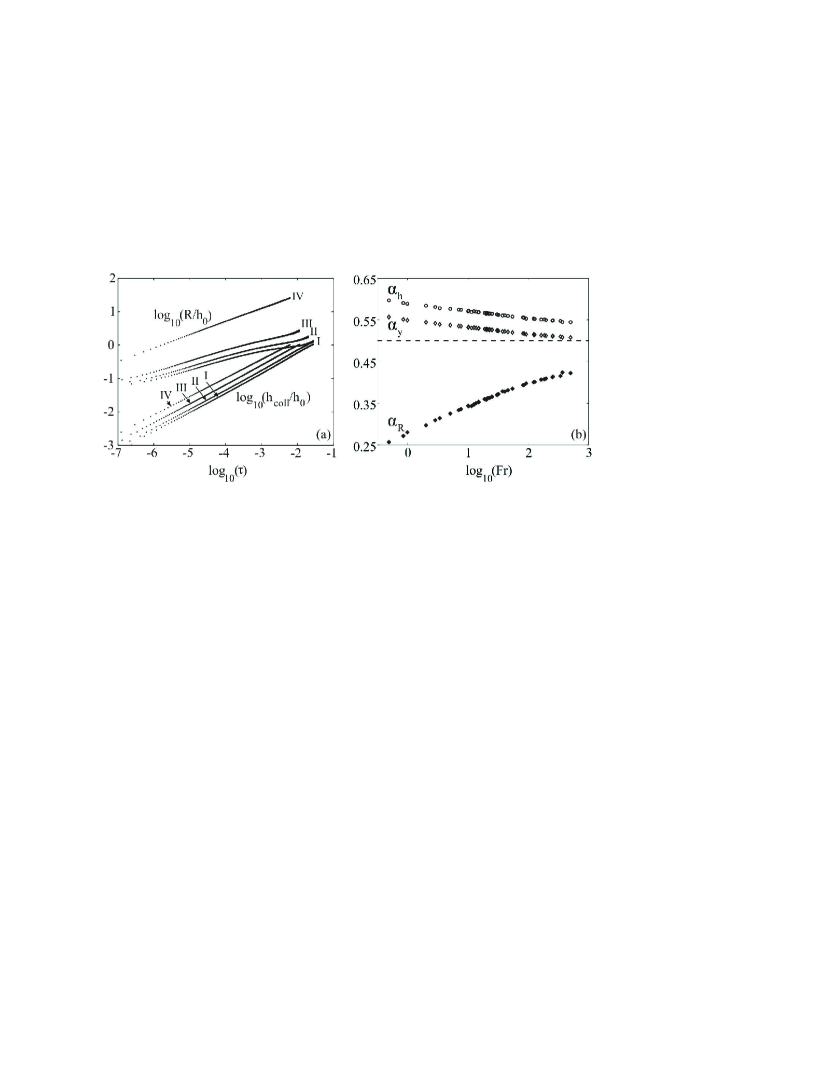
Figure 15: (a) Time-evolution of the neck radius at closure depth $h_{coll}(tau)$ and the radius of curvature $R(\tau)$ in the axial direction for $\text{Fr}=3.4$, $5.1$, $10.2$, and $200$. Both are found to follow a power law with respective exponents $\alpha_{h}$ and $\alpha_{R}$. (b) Power-law exponents $\alpha_{h}$ and $\alpha_{R}$ of the neck radius and radius of curvature as a function of the Froude number. Here we have added the exponents $\alpha_{y}$ which are corrected for the logarithmic factor in Eq. (34). In the large Fr limit, all exponents approach the Rayleigh-value of 1/2 [cf. Eq. (18)].

A.2 Cavity shape at pinch-off

If the pinch off would be self-similar, the free-surface profiles near the closure point at different times (Fig. 16a) would superpose when rescaled by any one characteristic length, e.g., the neck radius $h(\tau)$. Due to the different time-dependence of the neck radius and the radius of curvature, however, such an operation fails to collapse the void profiles onto a single shape. To characterize the free-surface shapes, one thus needs to consider the neck radius $h_{coll}(t)$ and the radius of curvature $R(t)$.

As was argued in Bergmann et al. (2006), if the radial dimension $r$ is scaled by $h_{coll}$, it follows from the locally parabolic shape and Eq. (35) that the axial dimension $z$ should be scaled by $\sqrt{h_{coll}R}$. Instead of using the actual length scales to rescale the profiles in Fig. 16b, we use the power laws that were obtained from the numerical simulations to collapse all experimental profiles onto a single curve. This signals once more the excellent agreement between the simulations and the experiment, as the scaling exponents are obtained from the simulations and the profiles from experiment.

As will be discussed in Appendix B, the axial position of the minimum radius $z_{min}$ moves down somewhat as the collapse progresses and it is therefore necessary to translate the profiles in the vertical direction to match the position of the minimum radius. For the inertially driven pinch off of a bubble from an underwater nozzle Thoroddsen et al. (2007) also find that two length scales are necessary to collapse the free surface profiles.

Recent theoretical calculations by Gordillo & Pérez-Saborid (2006) and Eggers et al. (2007) for the symmetric inertial pinch off of a single bubble (either initiated by surface tension or a straining flow) indicate that the scaling law for $h_{coll}(\tau)$ has an exponent which slowly varies with time, i.e., strictly speaking it does not scale. Our findings so far cannot confirm or disprove this theory, since our experiments and boundary integral simulations do not have sufficient temporal range to find the small deviations in the exponent. To escape the limitation of the experimental range set by the viscosity, surface tension, and air, the experiment should be scaled up to an unrealistic size (with a container size of over $10^{3}$ meters) to match the needed precision of at least 10 decades in time presented in the numerical calculations of Eggers et al. (2007).

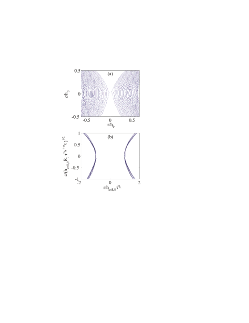
Figure 16: The profiles of the void obtained by experiments for $h_{0}=$ 30 mm and $V=1.0$ m/s (Fr $=3.4$). (a) Void profile obtained at different instances in time. (b) Void profile in which the radial and axial coordinates were rescaled with the powerlaws of $h_{coll}(t)$ and $\sqrt{h_{coll}(t)R(t)}$ respectively. Here, the numerically determined power–laws were used for the neck radius $h_{coll}(\tau)$ and the radius of curvature $R(\tau)$ (see main text).

Appendix B Minimal neck radius

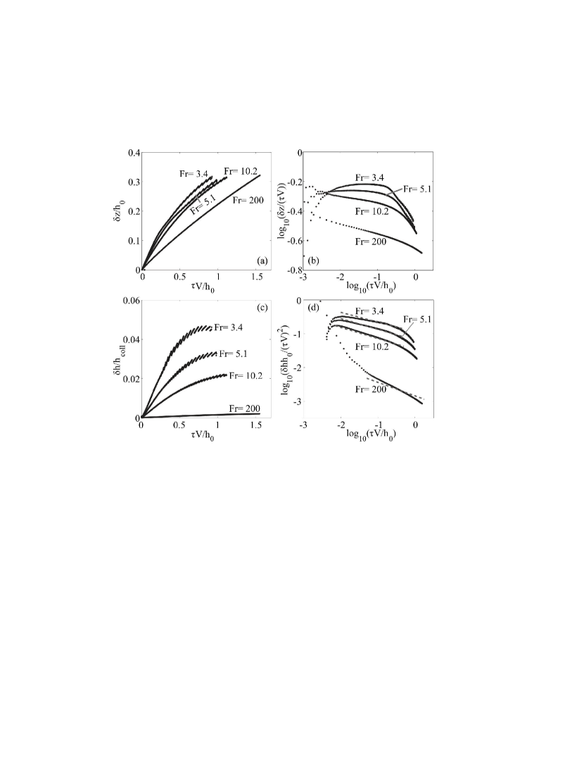
Figure 17: (a) The difference $\delta z(\tau)$ between the depth of the minimal radius $z_{min}(\tau)$ and the depth of closure $z_{coll}$ (both normalized by the disk radius $h_{0}$) as a function of the time interval $\tau$ (normalized by $h_{0}/V$) remaining until pinch–off for different Froude numbers. Each data series is obtained from the boundary integral simulations and starts when the minimal radius equaled the disk radius $h_{0}$. (b) Doubly logarithmic plot of the same data as (a), only now $\delta z$ is compensated by $\tau$ revealing an interval in which $\delta z$ is proportional to $\tau$ (showing as a horizontal line in the plot). (c) The difference $\delta h(\tau)=h_{coll}(\tau)-h_{min}(\tau)$ of the radius at closure depth $h_{coll}(\tau)$ and the minimal radius $h_{min}(\tau)$ of the cavity, normalized by $h_{coll}(\tau)$, as a function of $\tau$ (normalized by $h_{0}/V$) for different Froude numbers. Clearly, $\delta h/h_{coll}$ is smaller for increasing Froude number which results from the fact that the cavity shape becomes more cylindrical for high Fr. (d) Doubly logarithmic plot of the same data as in (c), only now $h_{coll}-h_{min}$ is compensated by $\tau^{2}$ to reveal the resultant scaling $\tau^{-\alpha_{R}}$ (see text). The dashed red lines are the scaling exponents $\alpha_{R}(\text{Fr})$ found by determining the time evolution of the radius of curvature in the axial direction through the procedure outlined in Bergmann et al. (2006) ($\alpha_{R}(\text{Fr=3.4})=0.29;\alpha_{R}(\text{Fr=5.1})=0.32;\alpha_{R}(\text{Fr=10.2})=0.33$; and $\alpha_{R}(\text{Fr=200})=0.40)$). The jumps in the data of Figures (a) and (c) are a result of the regridding routine in our boundary integral simulation and have no physical meaning.

Recently, a lot of attention has been given to the time evolution of the minimal cavity radius $h_{min}(\tau)$ at the closure depth and the (non-)universality of its scaling behavior approaching the pinch-off, see Gordillo et al. (2005), Bergmann et al. (2006), Gordillo & Pérez-Saborid (2006), and Eggers et al. (2007) (cf. also Appendix A). Especially in the theoretical analysis of Gordillo & Pérez-Saborid (2006) and Eggers et al. (2007) it is a key assumption that the dynamics is symmetric around the pinch-off point. In this Appendix we will show that in our setup this assumption is not satisfied, as the position of the minimum neck radius actually moves downwards in time.

In Figure 17a the difference $\delta z(\tau)$ between the depth at which the cavity radius is minimal $z_{min}(\tau)$ and the depth of closure $z_{coll}$ is plotted as a function of the time interval $\tau$ remaining until pinch–off for four different Froude numbers. Each data series is obtained from the boundary integral simulations and, as we focus on the behavior close to pinch–off, starts when the minimal radius is equal to the disk radius $h_{0}$.

We observe that the dynamics near pinch–off can be reasonably well described by a simple proportionality $\delta z\propto\tau$. This becomes even more clear if we compensate $\delta z$ by $\tau$ in a double logarithmic plot of the same data (Fig. 17b), which reveals a plateau in which $\delta z/\tau$ becomes independent of time, especially for the lower three Froude numbers.

As the pinch-off is approached, not only the depth of the minimal radius $z_{min}(\tau)$ converges to the depth of closure $z_{coll}$, but naturally also the minimal radius itself $h_{min}(\tau)$ approaches the radius at the depth of closure $h_{coll}(\tau)$ as can be seen in Fig. 17c. The relative difference $\delta h(\tau)$ between $h_{min}$ and $h_{coll}$ is seen to be smaller for increasing Froude number due to the cavity taking a more cylindrical shape at higher Froude number.

Since the cavity profile is locally parabolic close to the pinch–off point the approach of $h_{min}$ to $h_{coll}$ is described as:

$$\delta h(\tau)=\frac{[\delta z(\tau)]^{2}}{2R(\tau)}\,,$$ (36)

where $R(\tau)$ is the radius of curvature in the axial direction at the minimum neck radius.

This radius of curvature was found to exhibit power-law scaling in time with a Froude-dependent exponent $R(\tau)\propto\tau^{\alpha_{R}}$ (cf. Bergmann et al. (2006) and Appendix A, Fig. 15)which we can combine with the linear time dynamics found for $\delta z$ in Fig. 17. This leads to $h_{min}$ approaching $h_{coll}$ as

$$\delta h\propto\tau^{2-\alpha_{R}}.$$ (37)

Indeed, in Fig. 17d this scaling is confirmed for the lower Froude numbers. For the highest Froude number ($\text{Fr}=200$) the data seem to deviate from this scaling due to small deviations from $\delta z\propto\tau$ which are observed for this Froude number in Fig. 17b.

The final question we want to address in this section is whether it is possible to understand the relation $\delta z\propto\tau$ from the model. We start from Eq. (18) with $t_{coll}=\Delta t$ given by Eq. (25), i.e., for $t_{cross}<t<t_{coll}$

$$h(z,t)=\sqrt{2h_{0}\alpha_{ctra}V}\sqrt{\Delta t\small{(z)}\,\,-\,\,t\,\,}\,.$$ (38)

To find the depth of minimal radius we now have to compute the derivative of $h(z,t)$ to $z$ and equate to zero, or, equivalently

$$\frac{\partial}{\partial z}[h(z,t)^{2}]=2h_{0}\alpha_{ctra}V\left[\frac{\partial\Delta t}{\partial z}\right] = 0\qquad\Rightarrow$$ (39)

$$\frac{1}{V}-(\alpha_{expa}\beta_{expa}+\alpha_{ctra}\beta_{ctra})\frac{h_{0}V}{gz^{2}} = 0\,,$$ (40)

which leads to the conclusion that the depth of the minimal radius is always equal to the closure depth, i.e., independent of time (cf. Eq. (27)). Clearly this is in disagreement with the observations. This was to be expected as the translation of the depth of the minimal radius is quite small, typically an order of magnitude smaller than other length scales, e.g., the closure depth). We will therefore have to look for a second order effect.

To take the discussion one step further, we return to Fig. 12a, where we find that $\alpha_{ctra}$ slightly decreases with increasing Froude number. From this we can infer (at least qualitatively) that $\alpha_{ctra}$ also very slightly decreases with depth. This stands to reason, as $\alpha_{ctra}$ shows the same trend (in Fr) as $\alpha_{expa}$, which is the ratio of the initial expansion velocity of the cavity and the disk velocity. As at greater depth the hydrostatic pressure is larger it is expected that $\alpha_{expa}$ should decrease with depth.

Now letting $\alpha_{ctra}$ (and the other parameters $\alpha_{expa}$, $\beta_{expa}$, and $\beta_{ctra}$) depend on $z$ we have

$$\frac{\partial}{\partial z}[h(z,t)^{2}]=2h_{0}V\left(\frac{\partial\alpha_{ctra}}{\partial z}\right)\,\tau+2h_{0}V\alpha_{ctra}\small{(z)}\left(\frac{\partial\Delta t\small{(z)}}{\partial z}\right)=0\,.$$ (41)

For any fixed Froude number $\text{Fr}_{0}$ we can now Taylor expand $\partial\Delta t/\partial z$ around the closure depth $z_{coll}$ which leads to

$$\frac{\partial\Delta t}{\partial z}=\left(\frac{\partial\Delta t}{\partial z}\right)_{z_{coll}}+\,\,\,(\delta z)\left(\frac{\partial^{2}\Delta t}{\partial z^{2}}\right)_{z_{coll}}=\,\,\,(\delta z)\left(\frac{\partial^{2}\Delta t}{\partial z^{2}}\right)_{z_{coll}}\,,$$ (42)

as within the model the closure depth is defined by the condition $(\partial\Delta t/\partial z)_{z_{coll}}=0$ (see subsection 4.1). Recall that $\delta z=z-z_{coll}$. Combining the above two equations then leads to the following relation between $\delta z$ and $\tau$

$$\delta z=-\left[\frac{1}{\alpha_{ctra}}\left(\frac{\partial\alpha_{ctra}}{\partial z}\right)\left(\frac{\partial^{2}\Delta t}{\partial z^{2}}\right)^{-1}\right]_{z_{coll}}\tau\,,$$ (43)

where it is good to note that $\Delta t$ does not only directly depend on $z$, but also indirectly, through the parameters $\alpha_{ctra}$, $\alpha_{expa}$, $\beta_{expa}$, and $\beta_{ctra}$.

From the data presented in Fig. 12a we can perform a local second order fit to $\alpha_{ctra}$ as a function of $\sqrt{\text{Fr}}$ around $\sqrt{\text{Fr}_{0}}$. Assuming that the relation between closure depth and Froude number also holds near the closure depth, i.e., $z/h_{0}=C_{1}\sqrt{\text{Fr}}$ with $C_{1}\approx 1.10$ (see again subsection 4.1) we can translate this into a quadratic expression in $\delta z$

$$\alpha_{ctra}\approx\alpha_{ctra,\,0}+k_{1}\frac{\delta z}{h_{0}}+k_{2}\frac{(\delta z)^{2}}{h_{0}^{2}}\,,$$ (44)

and similarly for the other parameters $\alpha_{expa}$, $\beta_{expa}$, and $\beta_{ctra}$.

As an example we take $\text{Fr}_{0}=5.1$ for which we find $\alpha_{ctra,\,0}=0.56$, $k_{1}=-0.087$, and $k_{2}=0.038$. After a straightforward but quite lengthy calculation we evaluated the prefactor in Eq. (43) to give $\delta z/h_{0}\approx 0.20\tau V/h_{0}$. This is in the same direction and of the same order of magnitude as the result from our boundary integral simulation where we find $\delta z/h_{0}\approx 0.51\tau V/h_{0}$ (see Fig. 17a and b). Repeating this procedure for $\text{Fr}=10.2$ $\text{Fr}=200$ yields proportionality constants of $0.16$ and $0.074$ respectively, which correctly predict the downward trend with increasing Froude number that is also observed in the numerical simulation, where we find $0.42$ and $0.25$ respectively. Considering the large number of approximations made in this calculation and the subtlety of the effect the agreement is remarkable.

References

- Bergmann et al. (2006) Bergmann, R., Stijnman, M., Sandtke, M., van der Meer, D., Prosperetti, A. & Lohse, D. 2006 Giant bubble collapse. Phys. Rev. Lett. 96, 154505/1–4.
- Caballero et al. (2007) Caballero, G., Bergmann, R., van der Meer, D., Prosperetti, A. & Lohse, D. 2007 Role of air in granular jet formation. Phys. Rev. Lett. 99, 018001/1–4.
- Chen & Basaran (2002) Chen, A. & Basaran, O. 2002 A new method for significantly reducing drop radius without reducing nozzle radius in drop-on-demand drop production. Phys. Fluids 14, L1.
- Duclaux et al. (2007) Duclaux, V., Caillé, F., Duez, C., Ybert, C., Bocquet, L. & Clanet, C. 2007 Dynamics of transient cavities. J. Fluid Mech. 591, 1–19.
- Eggers et al. (2007) Eggers, J., Fontelos, M., Leppinen, D. & Snoeijer, J. 2007 Theory of the collapsing axisymmetric cavity. Phys. Rev. Lett. 98, 094502/1–4.
- Fedorchenko & Wang (2004) Fedorchenko, A. & Wang, A.-B. 2004 On some common features of drop impact on liquid surfaces. Phys. Fluids 16, 1349–1365.
- Gaudet (1998) Gaudet, S. 1998 Numerical simulation of circular disks entering the free surface of a fluid. Phys. Fluids 10, 2489–2499.
- Gekle et al. (2008) Gekle, S., van der Bos, A., Bergmann, R., van der Meer, D. & Lohse, D. 2008 Noncontinuous froude number scaling for the closure depth of a cylindrical cavity. Phys. Rev. Lett. 100, 084502/1–4.
- Gilbarg & Anderson (1948) Gilbarg, D. & Anderson, R. A. 1948 Influence of atmospheric pressure on the phenomena accompanying the entry of spheres into water. J. Appl. Phys. 19, 127–139.
- Glasheen & McMahon (1996) Glasheen, J. W. & McMahon, T. A. 1996 A hydrodynamic model of locomtion in the basilisk lizard. Nature 380, 340 – 342.
- Gordillo & Pérez-Saborid (2006) Gordillo, J. & Pérez-Saborid, M. 2006 Axisymmetric breakup of bubbles at high reynolds numbers. J. Fluid Mech. 562, 303–312.
- Gordillo et al. (2005) Gordillo, J., Sevilla, A., Rodriguez-Rodriguez, J. & Martinez-Bazan, C. 2005 Axisymmetric bubble pinch-off at high reynolds numbers. Phys. Rev. Lett. 95, 194501/1–4.
- de Jong et al. (2006a) de Jong, J., de Bruin, G., Reinten, H., van den Berg, M., Wijshoff, H., Versluis, M. & Lohse, D. 2006a Air entrapment in piezo-driven inkjet printheads. J. Acoust. Soc. Am. 120, 1257–1265.
- de Jong et al. (2006b) de Jong, J., Jeurissen, R., Borel, H., van den Berg, M., Wijshoff, H., Reinten, H., Versluis, M., Prosperetti, A. & Lohse, D. 2006b Entrapped air bubbles in piezo-driven inkjet printing: Their effect on the droplet velocity. Phys. Fluids 18, 121511–121517.
- Le (1998) Le, H. P. 1998 Progress and trends in ink-jet printing technology. J. Imag. Sci. Tech 42, 49–62.
- Lee et al. (1997) Lee, M., Longoria, R. & Wilson, D. 1997 Cavity dynamics in high-speed water entry. Phys. Fluids 9, 540–550.
- Liow et al. (1996) Liow, J.-L., Morton, D., Guerra, A. & Gray, N. 1996 In Howard Worner Inr. Symp. on injection in pyrometallurgy (ed. M. Nilmani & T. Lehner). Pennsylvania.
- Lohse et al. (2004) Lohse, D., Bergmann, R., Mikkelsen, R., Zeilstra, C., van der Meer, D., Versluis, M., van der Weele, K., van der Hoef, M. & Kuipers, H. 2004 Impact on soft sand: Void collapse and jet formation. Phys. Rev. Lett. 93, 198003/1–4.
- Morton et al. (2000) Morton, D., Liow, J.-L. & Rudman, M. 2000 An investigation of the flow regimes resulting from splashing drops. Phys. Fluids 12, 747–763.
- Oguz & Prosperetti (1990) Oguz, H. & Prosperetti, A. 1990 Bubble entrainment by the impact of drops on liquid surfaces. J. Fluid Mech. 219, 143–179.
- Oguz & Prosperetti (1993) Oguz, H. N. & Prosperetti, A. 1993 Dynamics of bubble-growth and detachment from a needle. J. Fluid Mech. 257, 111–145.
- Oguz et al. (1995) Oguz, H. N., Prosperetti, A. & Kolaini, A. R. 1995 Air entrapment by a falling water mass. J. Fluid Mech. 294, 181–207.
- Power & Wrobel (1995) Power, H. & Wrobel, L. C. 1995 Boundary integral methods in fluid mechanics. WIT Press (UK).
- Prosperetti (2002) Prosperetti, A. 2002 Drop surface interactions. Springer, CISM courses and lectures Nr. 456.
- Prosperetti et al. (1989) Prosperetti, A., Crum, L. & Pumphrey, H. 1989 Underwater noise of rain. J. Geophys. Res. 94, 3255–3259.
- Prosperetti & Oguz (1997) Prosperetti, A. & Oguz, H. 1997 Air entrainment upon liquid impact. Phil. Trans. R. Soc. Lond. A 355, 491–506.
- Rein (1993) Rein, M. 1993 Phenomena of liquid drop impact on solid and liquid surfaces. Fluid Dyn. Res. 12, 61–93.
- Royer et al. (2005) Royer, J., Corwin, E., Flior, A., Cordero, M.-L., Rivers, M., Eng, P. & Jaeger, H. 2005 Formation of granular jets observed by high-speed x-ray radiography. Nat. Phys. 1, 164–167.
- Thoroddsen & Shen (2001) Thoroddsen, S. & Shen, A. 2001 Granular jets. Phys. Fluids 13, 4–6.
- Thoroddsen et al. (2007) Thoroddsen, S. T., Etoh, T. G. & Takehara, K. 2007 Experiments on bubble pinch-off. Phys. Fluids 19, 042101–042129.
- Worthington (1908) Worthington, A. M. 1908 A study of splashes. London: Longman and Green.
- Worthington & Cole (1897) Worthington, A. M. & Cole, R. S. 1897 Impact with a liquid surface, studied by the aid of instantaneous photography. Phil. Trans. R. Soc. Lond. A 189, 137.