Abstract

We calculate all the four-photon helicity amplitudes at the one-loop level in a massive theory using multiple-cut methods. The amplitudes are derived in scalar QED, QED and $\textrm{QED}^{{\cal N}=1}$ theories. We will see the origin of rational terms. We extend the calculation to the simplest six-photon helicity amplitude where all photons have the same helicity.

1 Introduction

The light-by-light scattering is a good laboratory to find efficient methods to compute a massive loop multi-leg amplitude, because gauge invariance and IR/UV finiteness lead to enormous cancellations when we sum all the Feynman diagram. The first calculation of the four-photon amplitude in massive QED was done by Karplus and al. [1]. They straightforwardly calculated each Feynman diagram. Then B. de Tollis [2] computed the four-photon amplitude with Cutkosky rules. Ten years ago, Bern and Morgan calculated the four-gluon helicity amplitudes with a massive loop [3]. They used the two-cut unitarity methods in $n$ dimensions. Recently, Bern et al. calculated the two loop corrections QCD and QED to light-by-light scattering by fermion loops in the ultrarelativistic limit [4]. Then Binoth and al. [5] calculated the four-photon helicity amplitudes in QED, scalar QED, supersymmetric $\textrm{QED}^{{\cal N}=1}$ and $\textrm{QED}^{{\cal N}=2}$ in massless theory. They used a n-dimensional projection method. Two years ago, Brandhuber and al. calculated the four-gluon one loop helicity amplitudes with generalized unitarity cuts [6].

Here we want to compute the four-photon amplitude, in massive QED, with a recent method: the generalized unitarity cuts. Even at the energy of LHC, 14 TeV, the mass of heavy quark $t$ can have a significant effect. This article aims at explaining how to use new unitarity-cut methods in the case of massive theories. Here we apply this new technology for a $2\rightarrow 2$ process. However, the future project is to calculate easily some $2\rightarrow 4$ QCD processes, like $gg\rightarrow\overline{t}t\overline{t}t$ with heavy quarks, present in the background of LHC. The knowledge of the background is very important to detect new particles like Higgs.

In this paper, we calculate the four-photon amplitude at one loop order in three massive QED theories: scalar QED, QED and supersymmetric $\textrm{QED}^{{\cal N}=1}$. Our result agree with [4, 5]. We call $A^{scalar}_{4}$ (respectively $A^{spinor}_{4}$ and $A^{{\cal N}=1}_{4}$ ) the four-photon amplitude in scalar QED (respectively QED and supersymmetric $\textrm{QED}^{{\cal N}=1}$). We obtain very compact expressions contrary to Karplus and we can deduce easily the origin of the rational terms. Actually, we can link easily these three amplitudes with a supersymmetric decomposition. All diagrams of the four-photon amplitude in QED have the same pattern: four external photons coupled to a fermion loop. However, using the fact that degrees of freedom for internal lines can be added and subtracted [9, 10], we write the internal fermion as a supersymmetric contribution and a scalar:

$$f\ =\ -2\ s+(f+2s)\ \ \Rightarrow\ \ A^{fermion}_{4}\ =\ -2\ A^{scalar}_{4}+A^{{\cal N}=1}_{4}.$$ (1)

This formula is true for massless and massive theories. Moreover we point out that this formula $\left(\ref{supersymmetricdecomposition}\right)$ is true for any number of photons.

We calculate all $A^{scalar}_{4}$ helicity amplitudes with generalized unitarity cuts in sections $\ref{amplitudescalar++++},\ref{amplitudescalar-+++},\ref{amplitudescalar--++}$. Then, we use extensively the supersymmetric decomposition $\left(\ref{supersymmetricdecomposition}\right)$ to calculate the QED amplitude $A^{fermion}_{4}$ in section 4 and the amplitude $A^{{\cal N}=1}_{4}$ in section 6. Indeed, if we write the four-photon amplitude in QED, the supersymmetric decomposition imposes the pattern of the supersymmetric amplitude $A^{{\cal N}=1}_{4}$ function of magnetic moments. We don’t need to calculate all the supersymmetric diagrams. After, we discuss about the origin of the rational terms and the different cut-techniques in section 5. Finally we derive the most simple helicity amplitude of the six-photon amplitudes in Section 7.

But first, some notations and explanations on generalized unitary cuts will be introduced.

2 Notations and explanations

2.1 The structure of the amplitude $\gamma_{1}+\gamma_{2}+\gamma_{3}+\gamma_{4}\rightarrow 0$

We study the process $\gamma_{1}+\gamma_{2}+\gamma_{3}+\gamma_{4}\rightarrow 0$. The momenta of the ingoing photon called $i$ is $p_{i}^{\mu}$. In this paper we suppose that all the photons are on-shell, so we have the first relation $\forall i\in[1..4],\ p_{i}^{2}=0$. Diagrams at tree order are impossible and the first non vanishing order is one-loop order.

The QED Lagrangian contains one vertex, whereas the scalar QED Lagrangian gives us two vertices. We recall them in Appendix A. Therefore in QED we have six one-loop diagrams whereas in scalar QED we have twenty one one-loop diagrams. As we have only four external particles entering in the loop, the power counting tells us that individual diagrams are UV divergent. So we regularized the divergence in calculating loops in $n=4-2\epsilon$ dimensions. Nevertheless, thanks to gauge invariance, the sum over all diagrams has no UV divergences. So we have to observe compensations. Moreover, as we suppose that the four photons are on-shell, therefore we decide to decompose the amplitudes $A^{spinor}_{4}$, $A^{scalar}_{4}$ and $A^{{\cal N}=1}_{4}$ on a basis of master integrals in $n$ and $n+2$ dimensions:

$$A_{4}=\sum_{i\in{1,2,3,4}}\left(a_{i}{I_{4}^{n+2}}_{i}+b_{i}{I_{3}^{n}(\textrm{1mass})}_{i}+c_{i}{I_{2}^{n}(\textrm{1mass})}_{i}\right)+\textrm{rational terms},$$ (2)

where $I_{4}^{n+2}$ is the no external mass box in $n+2$ dimensions, $I_{3}^{n}(\textrm{1mass})$ is the three-point function with one external mass and $I_{2}^{n}(\textrm{{1mass}})$ is the two-point function with one external mass. The exact definition of $I_{4}^{n+2}$, $I_{3}^{n}(\textrm{1mass})$ and $I_{2}^{n}$ can be found, for example in [3, 6, 7, 8]; nevertheless to be self consistent we recall them in Appendix C. The interest of this basis of master integrals, is to separate IR/UV, rational and analytic terms. But this basis is not unique. $I_{4}^{n+2}$ has an analytic structure with polylogarithms whereas the IR divergences, in massless theories are carried by the function $I_{3}^{n}(1m)$ and the UV one, in massless and massive theories by the function $I_{2}^{n}$. Each diagram is UV divergent so each diagram has scalar bubbles $I_{2}^{n}$, but the amplitude (sum of diagrams) is UV finite so we expect to have compensations between the different scalar bubbles to eliminate the divergences.

The amplitude is totally defined by the coefficients $a_{i},b_{i},c_{i}$ and the rational terms. To calculate all these coefficients, we use the spinor formalism and the method of the helicity amplitudes.

2.2 Spinor formalism and helicity amplitudes

We use the spinor helicity formalism developed in  [11]. For the spinorial product, we introduce the following notation:

$$\langle p_{a}-|p_{b}+\rangle =\langle ab\rangle$$ (3)

$$\langle p_{a}+|p_{b}-\rangle =[ab]$$ (4)

$$\langle p_{a}-|\mbox{$\not{\!p_{b}}$}|p_{c}-\rangle =\langle abc\rangle=[cba]=\langle p_{c}+|\mbox{$\not{\!p_{b}}$}|p_{a}+\rangle=[p_{c}p_{b}]\langle p_{b}p_{a}\rangle$$ (5)

$$\langle p_{a}+|\mbox{$\not{\!p_{b}}$}\mbox{$\not{\!p_{c}}$}|p_{d}-\rangle =[abcd]=-[dcba]=-\langle p_{d}+|\mbox{$\not{\!p_{c}}$}\mbox{$\not{\!p_{b}}$}|p_{a}-\rangle.$$ (6)

Moreover we introduce the classical Mandelstam variables :

$$s\ =\ s_{12}\ =\ \langle 12\rangle[21]\quad t\ =\ s_{14}\ =\ \langle 14\rangle[41]\quad u\ =\ s_{13}\ =\ \langle 13\rangle[31].$$ (7)

All coefficients $a_{i},b_{i},c_{i}$ and rational terms are described as products of spinor and Mandelstam variables.

We calculate all helicity amplitudes. A photon has two helicity states $\sigma=\pm$. The amplitude is the sum of all helicity states.

$$A_{4}\ =\ \displaystyle\sum_{\sigma_{1}=\pm,\sigma_{2}=\pm,\sigma_{3}=\pm,\sigma_{4}=\pm}A_{4}\left(\sigma_{1},\sigma_{2},\sigma_{3},\sigma_{4}\right).$$ (8)

As we have two helicity states per external photons and four external photons, so the amplitude $A_{4}$ is the sum of $2^{4}=16$ helicity states. However they are not all independent. In fact we have only three independent helicity states $A_{4}(++++),A_{4}(-+++)$ and $A_{4}(--++)$. Others are obtained by permutations and parity.

It is necessary to introduce the polarisation vectors of the external photons. The advantage of the helicity amplitudes is that we can express easily all the photon-polarisation vectors with spinors. Those expressions come from [11]:

$${\varepsilon_{1}^{+}}^{\mu}\ =\ \frac{\langle R\gamma^{\mu}1\rangle}{\sqrt{2}\langle R1\rangle}\quad\quad{\varepsilon_{1}^{-}}^{\mu}\ =\ \frac{[r\gamma^{\mu}1]}{\sqrt{2}[1r]},$$ (9)

where $|R\rangle$ and $|r\rangle$ are two arbitrary light-like vectors. Before giving results on $A_{4}^{scalar}$, we give explanations and notations on regularization, propagators and integrals.

2.3 The regularization scheme and notation of integrals

All diagrams have the same pattern and all are UV divergent. To regularize, we put the loop momentum $Q^{\mu}$ in $n=4-2\epsilon$ dimensions. Capital letters describe vectors in $n$ dimensions whereas small letters describe vectors in four dimensions. So we decompose the loop momentum $Q^{\mu}=q^{\mu}+\mu^{\mu}$ with $q^{\mu}$ the four-dimensional part and $\mu^{\mu}$ the $-2\epsilon$ part. The four-dimensional space and the $-2\epsilon$-dimensional space are orthogonal so one has: $Q^{2}=q^{2}-\mu^{2}$. And we operate in the “four-dimensional helicity scheme”, in which all external momenta are in four dimensions. In $n$ dimensions, we take the prescription where the propagators are defined by:

fermion $$\quad\quad i\frac{\mbox{$\not{\!Q}$}+m}{Q^{2}-m^{2}+i\lambda}\ =\ i\frac{\mbox{$\not{\!Q}$}+m}{q^{2}-\mu^{2}-m^{2}+i\lambda}\ =\ i\frac{\mbox{$\not{\!Q}$}+m}{D^{2}_{q}},$$ (10)

scalar $$\quad\quad i\frac{1}{Q^{2}-m^{2}+i\lambda}\ =\ i\frac{1}{q^{2}-\mu^{2}-m^{2}+i\lambda}\ =\ i\frac{1}{D^{2}_{q}}.$$ (11)

The formulas $\left(\ref{propagatorfermions},\ref{propagatorscalar}\right)$ show that the running particle seems to have a mass: $m^{2}+\mu^{2}$. We will observe this phenomena in the analytic expression of the amplitude $A_{4}$. The generalized unitarity-cut imposes the calculation of some trees in $n$ dimensions, where the running particle enters with a mass $m^{2}+\mu^{2}$. The $n$-dimensional calculation introduces some integrals with powers of $\mu$ in the numerator; those integrals are called extra-dimension integrals. We express, in Appendix D.2, those integrals in terms of higher dimension loop scalar integrals. But here we give the definitions of some scalar integrals and extra-dimension scalar integrals, used in this paper [3]:

$$I_{N}^{n}\ =\ \frac{1}{i\pi^{n/2}}\int d^{n}Q\frac{1}{D_{1}^{2}...D_{N}^{2}},$$ (12)

$$J_{N}^{n}\ =\ \frac{1}{i\pi^{n/2}}\int d^{n}Q\frac{m^{2}+\mu^{2}}{D_{1}^{2}...D_{N}^{2}},$$ (13)

$$K_{N}^{n}\ =\ \frac{1}{i\pi^{n/2}}\int d^{n}Q\frac{\left(m^{2}+\mu^{2}\right)^{2}}{D_{1}^{2}...D_{N}^{2}}.$$ (14)

We explain in Section 5.2 the origin of those extra scalar integrals. In our convention, we ignore a factor $K=i(4\pi)^{-n/2}$ in front of each scalar integral of the amplitude, and we reintroduce it, in the final result. In the following, we often add arguments to the integral to denote the order of photons entering the loop. We give the definition of those arguments:

$$I_{4}^{n}(abcd)\ =\ I_{4}^{n}\left(s_{ab},s_{ad}\right)\ =\ \parbox{56.9055pt}{\includegraphics[width=56.9055pt]{definitionI4.eps}}$$

$$I_{3}^{n}(s_{cd})\ =\ \parbox{56.9055pt}{\includegraphics[width=56.9055pt]{definitionI3.eps}}$$

$$I_{2}^{n}(s_{cd})\ =\ I_{2}^{n}(s_{ab})\ =\ \parbox{56.9055pt}{\includegraphics[width=56.9055pt]{definitionI2.eps}}$$ (15)

In Appendix C, we give some analytic expressions in terms of polylogarithms of those massive and massless scalar integrals.

We decide to express the amplitude $A^{fermion/scalar/{\cal N}=1}$ as a combination of master integrals $\left(\ref{decomposition}\right)$. To calculate the different coefficients in front of each master integral, we use the generalized unitarity-cut in $n$ dimensions, which we recall in the next subsection.

2.4 Generalized unitarity-cuts

The unitarity cut method come from the Cutkosky rules [12]. In the last ten years, there has been an intense development around the unitarity-cuts and several generalizations have been made. The first generalization of those rules is that we can cut not only two propagators but also three [13, 14] or four propagators [15, 16, 17]. But we will see that the more we cut propagators, the more we loose information. However, the more we cut propagators, the more the amplitude is simple to calculate. The second generalization is to evaluate the loop integral in $n=4-2\epsilon$ dimensions [3], which was improved in [18]. The four-dimension cuts are very efficient to calculate coefficients in front of structures but the extra-dimensional cuts are powerful to calculate the rational terms. We will see a link between extra-dimensions and rational terms [19, 20]. But the generalization of this link is not so obvious for a general amplitude. Another extension, which has recently be done, is the generalization of the unitarity cuts to massive theories. In [3], we find the calculation of four-gluon amplitudes at one loop in massive theory with the two-cut techniques. And recently, the unitarity-cut techniques in massive theories was generalized to three and four-cut techniques [21]. Finally, a few months ago, Papadopoulos and al. gave a general method to calculate each coefficient in front of the master integrals [22], extended by Forde [23, 24].

The Cutkosky rules [12] require to consider an invariant or a channel, constituted of several consecutive legs. Consider a loop amplitude, called $A$. One first computes the discontinuities across branch cuts (imaginary parts) by evaluating a phase space integral. The imaginary part of the amplitude is the sum over all the discontinuities:

$$2\ \textrm{Im}\left(A_{4}^{scalar}(++++)\right)\ =\ \sum_{i\in\textrm{channel}}\textrm{Disc}_{s_{i}}A.$$ (16)

The discontinuity in a channel can be computed by replacing the propagators separating the set of legs by delta functions:

$$\frac{i}{D_{i}^{2}}\ \rightarrow\ 2\pi\ \delta^{(+)}\left(D_{i}^{2}\right).$$ (17)

The real part is then reconstructed via a dispersion relation. The existence of a linear combination of scalar integrals allows us to avoid this reconstruction explicitly. We perform the cut calculation a bit differently. Consider the loop amplitude, with a cut in the channel: $s_{12}$ $\left(\textrm{Fig.}\ref{Figure1}\right)$. We compute the discontinuity $\textrm{Disc}_{s_{12}}\left(A\right)$. It is convenient to replace the phase-space integral with an unrestricted loop momentum integral which has the correct branch cuts $\left(\ref{feynmancoupure}\right)$. In this integral $\left(\ref{feynmancoupure}\right)$, the tree-amplitudes are kept on-shell. Then we decompose the discontinuity $\textrm{Disc}_{s_{12}}\left(A\right)$ as a linear combination of scalar cut-integrals in this channel $\left(\ref{decompositioncoupure}\right)$. The reconstruction of the amplitude is hidden in the rebuilding of the scalar integrals.

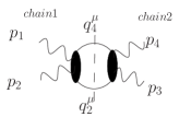
Figure 1: Fermion loop with a cut in the channel $s_{12}$.

$$\textrm{Disc}_{s_{12}}\left(A\right) \ =\ \left(2\pi\right)^{2}\int\frac{d^{n}Q}{\left(2\pi\right)^{n}}\ \delta^{(+)}(D_{2}^{2})\ A_{tree}(2)\ \delta^{(+)}(D_{4}^{2})\ A_{tree}(1)$$ (18)

$$\ =\ \int\frac{d^{n}Q}{\left(2\pi\right)^{n}}\frac{i}{D_{2}^{2}}A_{tree}(2)\left.\frac{i}{D_{4}^{2}}A_{tree}(1)\right|_{s_{12}}$$ (19)

$$\ =\ \sum_{i}c_{i}\left.I_{i}^{n}\right|_{s_{12}}=\sum_{i}c_{i}\ \textrm{Disc}_{s_{12}}\left(I_{i}^{n}\right).$$ (20)

From this, we can write:

$$A\ =\ \sum_{i}c_{i}\ I_{i}^{n}+\Delta.$$ (21)

In the term $\Delta$, there is a combination of scalar integrals which cannot have a cut in the channel $s_{12}$. To obtain the coefficient in front of all scalar integrals, we have to consider cutting amplitudes in all channels $\left(s_{12},s_{13},s_{14}\right)$. In the following, we note:

$$2\pi\delta^{\left(+\right)}\ \equiv\ \delta.$$ (22)

We introduce a notation to label the number of cuts and the channels.“$\textrm{Disc}_{2,s}$” means cutting the two internal lines in channel “$s$”. Cutting a third internal in all possible ways leads to “$\textrm{Disc}_{3,s}$”, while cutting the two remaining lines leads to “$\textrm{Disc}_{4}$”, in which there is no need to specify the channel. We denote $\textrm{Disc}_{N}=\sum_{i\in\textrm{channel}}\textrm{Disc}_{N,s_{i}},N=2,3$.

We are going to calculate all the helicity amplitudes with two, three and four-cut techniques in $n=4-2\epsilon$ dimensions for massive theories, and then we compare all those techniques. Now, as we have given the definition of all objects used in this paper, we are going to calculate the first helicity amplitude $A_{4}^{scalar}(1^{+},2^{+},3^{+},4^{+})$ in the next section.

3 $A_{4}^{scalar}$ helicity amplitudes

3.1 $A_{4}^{scalar}(1^{+},2^{+},3^{+},4^{+})$ helicity amplitude

3.1.1 Four-cut technique

The four-cut technique [15, 16, 17] says that we cut all four propagators $D_{i}^{2},\ i=[1..4]$. We have:

$$\textrm{Disc}_{4}\left(A_{4}^{scalar}(++++)\right)=\frac{1}{4}\sum_{\sigma(1,2,3,4)}\parbox{56.9055pt}{\includegraphics[width=56.9055pt]{4++++4cuts.eps}}.$$

We define the loop momenta of propagators as $Q_{i}=Q_{i-1}+p_{i}$ and $Q_{0}=Q_{4}$. Using Feynman rules, we compute the discontinuity $\textrm{Disc}\left(A_{4}^{scalar}(++++)\right)$:

$$\textrm{Disc}_{4}\left(A_{4}^{scalar}(++++)\right)=\displaystyle\frac{(-2ie)^{4}}{\sqrt{2}^{4}} \sum_{\sigma(2,3,4)}\int d^{n}Q\frac{\langle RQ_{1}1\rangle}{\langle R1\rangle}\frac{\langle RQ_{2}2\rangle}{\langle R2\rangle}$$

$$\frac{\langle RQ_{3}3\rangle}{\langle R3\rangle}\frac{\langle RQ_{4}4\rangle}{\langle R4\rangle}\delta\left(D_{1}^{2}\right)\delta\left(D_{2}^{2}\right)\delta\left(D_{3}^{2}\right)\delta\left(D_{4}^{2}\right).$$ (23)

As the four-dimensional and the $-2\epsilon$-dimensional spaces are orthogonal, therefore, the spinor product can be simplified: $\langle RQ_{2}2\rangle=\langle Rq_{2}2\rangle+\langle R\mu 2\rangle=\langle Rq_{2}2\rangle$. In the following, we do this simplification each time it is possible and then we use the fact that all propagators are on-shell to simplify eq. $\left(\ref{M++++scamasse4cuts}\right)$. We use the first on-shell tree computed in Appendix F. This tree has only two photons, so we split the integrand into two groups of photons $\left(p_{1},p_{2}\right)$ and $\left(p_{3},p_{4}\right)$, and we apply the formula $\left(\ref{arbre1++}\right)$ for the two groups of photons. The discontinuity $\left(\ref{M++++scamasse4cuts}\right)$ directly becomes:

$$\textrm{Disc}_{4}\left(A_{4}^{scalar}(++++)\right) =\displaystyle(e\sqrt{2})^{4}\sum_{\sigma(2,3,4)}\frac{[12][34]}{\langle 12\rangle\langle 34\rangle}\int d^{n}Q\left(\mu^{2}+m^{2}\right)^{2}\delta\left(D_{1}^{2}\right)\delta\left(D_{2}^{2}\right)\delta\left(D_{3}^{2}\right)\delta\left(D_{4}^{2}\right)$$ (24)

$$=\displaystyle(e\sqrt{2})^{4}\sum_{\sigma(2,3,4)}\frac{[12][34]}{\langle 12\rangle\langle 34\rangle}\textrm{Disc}_{4}\left(\int d^{n}Q\frac{\left(\mu^{2}+m^{2}\right)^{2}}{D_{1}^{2}D_{2}^{2}D_{3}^{2}D_{4}^{2}}\right)$$ (25)

$$=\displaystyle(e\sqrt{2})^{4}\sum_{\sigma(2,3,4)}\frac{[12][34]}{\langle 12\rangle\langle 34\rangle}\textrm{Disc}_{4}\left(K_{4}^{n}(1234)\right).$$ (26)

3.1.2 Three-cut technique

The three-cut technique imposes three propagators on-shell. So in the case of the four-photon amplitudes, we have four branch cuts per four-point diagram, only one branch cut per three-point diagram and zero branch cut per two-point diagram. But actually, as the four photons are on-shell, we have only two invariants per four-point diagrams, and therefore only two independent branch cuts. So we divide the result by two. Moreover we collect diagrams to construct set of gauge invariant trees, so we divide again per two. The discontinuity $\textrm{Disc}_{3}\left(A_{4}^{scalar}(++++)\right)$ is:

$$\textrm{Disc}_{3}\left(A_{4}^{scalar}(++++)\right)= \ \frac{1}{2}\frac{1}{2}\frac{1}{4}\sum_{\sigma(1,2,3,4)}\left(\parbox{56.9055pt}{\includegraphics[width=56.9055pt]{4++++3cuts1.eps}}+\parbox{56.9055pt}{\includegraphics[width=56.9055pt]{4++++3cuts2.eps}}\right)$$

$$+\frac{1}{2}\frac{1}{2}\frac{1}{4}\sum_{\sigma(1,2,3,4)}\left(\parbox{56.9055pt}{\includegraphics[width=56.9055pt]{4++++3cuts3.eps}}+\parbox{56.9055pt}{\includegraphics[width=56.9055pt]{4++++3cuts4.eps}}\right).$$

In the first group, for example, $D_{1}^{2}$ is the propagator between the two photons $p_{1}$ and $p_{2}$ but we should not forget the diagram with the four-point vertex. There are three diagrams in each group. Thanks to permutations, all groups of cut-diagrams are the same, so the discontinuity becomes:

$$\textrm{Disc}_{3}\left(A_{4}^{scalar}(++++)\right)=\frac{1}{4}\sum_{\sigma(1,2,3,4)}\parbox{56.9055pt}{\includegraphics[width=56.9055pt]{4++++3cuts.eps}}.$$ (27)

So using the Feynman rules, the discontinuity $\textrm{Disc}_{3}\left(A_{4}^{scalar}(++++)\right)$ is:

$$\textrm{Disc}_{3}\left(A_{4}^{scalar}(++++)\right)=\displaystyle\frac{(-i\sqrt{2}e)^{4}}{4}\sum_{\sigma(1,2,3,4)} \int d^{n}Q\left(\sum_{\sigma(1,2)}\frac{\langle Rq_{1}1\rangle}{\langle R1\rangle}\frac{i}{D_{1}^{2}}\frac{\langle Rq_{2}2\rangle}{\langle R2\rangle}\right)$$

$$\left(\frac{\langle Rq_{3}3\rangle}{\langle R3\rangle}\frac{\langle Rq_{4}4\rangle}{\langle R4\rangle}\right)\delta\left(D_{2}^{2}\right)\delta\left(D_{3}^{2}\right)\delta\left(D_{4}^{2}\right).$$ (28)

We use the expression of the on-shell tree $\left(\ref{arbre1++}\right)$ for the second group $(p_{3},p_{4})$. For the first group of photons $(p_{1},p_{2})$, the propagators around this group are on shell, but the propagator joining the two photons are not on-shell, so we use $\left(\ref{arbre2++}\right)$:

$$\sum_{\sigma(1,2)}\frac{\langle Rq_{1}1\rangle}{\langle R1\rangle}\frac{i}{D_{1}^{2}}\frac{\langle Rq_{2}2\rangle}{\langle R2\rangle}\ =\ -\left(\mu^{2}+m^{2}\right)\frac{[12]}{\langle 12\rangle}\sum_{\sigma(1,2)}\frac{i}{D_{1}^{2}}.$$ (29)

Inserting $\left(\ref{arbre1++}\right)$ and $\left(\ref{arbre2++++scamasse3cuts}\right)$ in $\left(\ref{M++++scamasse3cuts}\right)$, the discontinuity $\textrm{Disc}_{3}\left(A_{4}^{scalar}(++++)\right)$ becomes:

$$\textrm{Disc}_{3}\left(A_{4}^{scalar}(++++)\right) =\frac{(e\sqrt{2})^{4}}{4}\displaystyle\sum_{\sigma(1,2,3,4)}\frac{[12][34]}{\langle 12\rangle\langle 34\rangle}\int d^{n}Q\left(\mu^{2}+m^{2}\right)^{2}\sum_{\sigma(1,2)}\frac{i}{D_{1}^{2}}\delta\left(D_{2}^{2}\right)\delta\left(D_{3}^{2}\right)\delta\left(D_{4}^{2}\right)$$ (30)

$$=\displaystyle(e\sqrt{2})^{4}\sum_{\sigma(2,3,4)}\frac{[12][34]}{\langle 12\rangle\langle 34\rangle}\left(\textrm{Disc}_{3,s_{12}}\left(K_{4}^{n}\left(1234\right)\right)+\textrm{Disc}_{3,s_{14}}\left(K_{4}^{n}(1234)\right)\right)$$ (31)

$$=\displaystyle(e\sqrt{2})^{4}\sum_{\sigma(2,3,4)}\frac{[12][34]}{\langle 12\rangle\langle 34\rangle}\textrm{Disc}_{3}\left(K_{4}^{n}\left(1234\right)\right).$$ (32)

In the last step we have gathered the two branch cuts of the scalar integrals $K_{4}^{n}$ to rebuild the entire discontinuity. Indeed the computation could be more simple. Consider a discontinuity with several branch cuts. The self consistency of the unitarity says that we find the same coefficients in front of all branch cuts of each scalar integral of this discontinuity. Actually, we need to calculate only the coefficient in front of one branch cut of each scalar integral of the discontinuity.

3.1.3 Two-cut technique

This time, only two propagators are on-shell. As we have on-shell photons, we have only two channels per diagram. Therefore we have two branch cuts and the imaginary part of the amplitude is the sum of the discontinuity of the two branch cuts. So, for each diagram, we decide to cut the propagators $D_{2}^{2},D_{4}^{2}$ and then we cut the propagators $D_{1}^{2},D_{3}^{2}$. Finally regrouping diagrams with the same cuts to make trees, we obtain:

$$2\ \textrm{Im}\left(A_{4}^{scalar}(++++)\right)=\textrm{Disc}_{2}\left(A_{4}^{scalar}(++++)\right)=\frac{1}{4}\sum_{\sigma(2,3,4)}\left(\parbox{56.9055pt}{\includegraphics[width=56.9055pt]{4++++2cuts.eps}}+\parbox{56.9055pt}{\includegraphics[width=56.9055pt]{4++++2cuts2.eps}}\right).$$ (33)

The numerical factor $\frac{1}{4}$ comes from the fact that we have gathered diagrams to create gauge invariant trees. We point out, thanks to permutations, the two groups of cut-integrals are the same. Therefore the discontinuity $\textrm{Disc}_{2}\left(A_{4}^{scalar}(++++)\right)$ is written:

$$\textrm{Disc}_{2}\left(A_{4}^{scalar}(++++)\right)=\displaystyle\frac{1}{2}\sum_{\sigma(2,3,4)}(-i\sqrt{2}e)^{4}\int d^{n}Q \left(\sum_{\sigma(1,2)}\frac{\langle Rq_{1}1\rangle}{\langle R1\rangle}\frac{i}{D_{1}^{2}}\frac{\langle Rq_{2}2\rangle}{\langle R2\rangle}\right)$$

$$\displaystyle*\left(\sum_{\sigma(3,4)}\frac{\langle Rq_{3}3\rangle}{\langle R3\rangle}\frac{i}{D_{3}^{2}}\frac{\langle Rq_{4}4\rangle}{\langle R4\rangle}\right)\delta\left(D_{2}^{2}\right)\delta\left(D_{4}^{2}\right).$$ (34)

Using $\left(\ref{arbre2++}\right)$, to simplify the two trees in $\left(\ref{M++++scamasse2cuts}\right)$, the discontinuity $\textrm{Disc}_{2}\left(A_{4}^{scalar}(++++)\right)$ becomes:

$$\textrm{Disc}_{2}\left(A_{4}^{scalar}(++++)\right) =\frac{(e\sqrt{2})^{4}}{2}\displaystyle\sum_{\sigma(2,3,4)}\frac{[12][34]}{\langle 12\rangle\langle 34\rangle}\int d^{n}Q\left(\mu^{2}+m^{2}\right)^{2}\sum_{\sigma(1,2)}\frac{i}{D_{1}^{2}}\sum_{\sigma(3,4)}\frac{i}{D_{3}^{2}}\delta\left(D_{2}^{2}\right)\delta\left(D_{4}^{2}\right)$$ (35)

$$=\displaystyle 2(e\sqrt{2})^{4}\sum_{\sigma(2,3,4)}\frac{[12][34]}{\langle 12\rangle\langle 34\rangle}\textrm{Disc}_{2,s_{12}}\left(K_{4}^{n}\left(1234\right)\right).$$ (36)

We have one branch cut of the scalar integrals. But we want to reconstruct the entire discontinuity of the scalar integral $K_{4}^{n}$. Using the conservation of energy-momentum of external moments, $\frac{[12][34]}{\langle 12\rangle\langle 34\rangle}$ is invariant by permutation. So we can split the amplitude in two equal terms. We transform, thanks to permutations, one of this term to obtain the second branch cut, and the discontinuity of the scalar integral appears:

$$\textrm{Disc}_{2}\left(A_{4}^{scalar}(++++)\right) =(e\sqrt{2})^{4}\sum_{\sigma(2,3,4)}\frac{[12][34]}{\langle 12\rangle\langle 34\rangle}\left(\textrm{Disc}_{2,s_{12}}\left(K_{4}^{n}\left(1234\right)\right)+\textrm{Disc}_{2,s_{14}}\left(K_{4}^{n}\left(1234\right)\right)\right)$$ (37)

$$=(e\sqrt{2})^{4}\sum_{\sigma(2,3,4)}\frac{[12][34]}{\langle 12\rangle\langle 34\rangle}\textrm{Disc}_{2}\left(K_{4}^{n}\left(1234\right)\right).$$ (38)

With this last discontinuity we reconstruct directly the helicity amplitude $A_{4}^{scalar}(++++)$ by transform the discontinuity of each scalar integral to the scalar integral. We multiply the result by the factor $K=i(4\pi)^{-n/2}$:

$$A^{scalar}_{4}(++++)=i\frac{(e\sqrt{2})^{4}}{(4\pi)^{n/2}}\sum_{\sigma(2,3,4)}\frac{[12][34]}{\langle 12\rangle\langle 34\rangle}K_{4}^{n}\left(1234\right)=\displaystyle 4i\alpha^{2}\sum_{\sigma(2,3,4)}\frac{[12][34]}{\langle 12\rangle\langle 34\rangle}K_{4}^{n}\left(1234\right),$$ (39)

where $\alpha=e^{2}/4\pi$. The reconstruction of scalar integrals is automatic, we don’t need dispersive relation. There is full agreement with [3].

3.2 $A_{4}^{scalar}(1^{-},2^{+},3^{+},4^{+})$ helicity amplitude

3.2.1 Four-cut technique

The four-cut technique sets the four propagators $D_{i}^{2},\ i=[1..4]$ on-shell:

$$\textrm{Disc}_{4}\left(A_{4}^{scalar}(-+++)\right)=\frac{1}{4}\sum_{\sigma(1,2,3,4)}\parbox{56.9055pt}{\includegraphics[width=56.9055pt]{4-+++4cuts.eps}}.$$

So the discontinuity $\textrm{Disc}_{4}\left(A_{4}^{scalar}(-+++)\right)$ is:

$$\textrm{Disc}_{4}\left(A_{4}^{scalar}(-+++)\right)=(-i\sqrt{2}e)^{4}\sum_{\sigma(2,3,4)}\int d^{n}Q\frac{[rq_{1}1]}{[1r]}\frac{\langle Rq_{2}2\rangle}{\langle R2\rangle}\frac{\langle Rq_{3}3\rangle}{\langle R3\rangle}\frac{\langle Rq_{4}4\rangle}{\langle R4\rangle}\delta\left(D_{1}^{2}\right)\delta\left(D_{2}^{2}\right)\delta\left(D_{3}^{2}\right)\delta\left(D_{4}^{2}\right).$$ (40)

We split the integrand in two groups of photons: $\left(p_{1},p_{2}\right)$ and $\left(p_{3},p_{4}\right)$. As the helicity of the two photons of the first group are different, therefore we use $\left(\ref{arbre-+}\right)$ in the limit of all propagators on-shell:

$$\frac{[rq_{1}1]}{[1r]}\displaystyle\frac{\langle Rq_{2}2\rangle}{\langle R2\rangle}\ =\ \displaystyle\lim_{D_{1}^{2},D_{3}^{2}\rightarrow 0}\left(\ref{arbre-+}\right)\ =\ -\frac{1}{\langle 231\rangle}\left(\langle 1q_{2}232\rangle+\left(\mu^{2}+m^{2}\right)[231]\right),$$ (41)

and for the second group of photons, we use the relation $\left(\ref{arbre1++}\right)$. The discontinuity $\left(\ref{M-+++scamasse4cuts}\right)$ becomes:

$$\textrm{Disc}_{4} \left(A_{4}^{scalar}(-+++)\right)\ =\displaystyle\ (e\sqrt{2})^{4}\sum_{\sigma(2,3,4)}\frac{[34][231]}{\langle 34\rangle\langle 231\rangle}\int d^{n}Q\left(\mu^{2}+m^{2}\right)^{2}\delta\left(D_{1}^{2}\right)\delta\left(D_{2}^{2}\right)\delta\left(D_{3}^{2}\right)\delta\left(D_{4}^{2}\right)$$

$$\displaystyle+\ (e\sqrt{2})^{4}\sum_{\sigma(2,3,4)}\frac{[34]}{\langle 34\rangle\langle 231\rangle}\int d^{n}Q\langle 1q_{2}232\rangle\left(\mu^{2}+m^{2}\right)\delta\left(D_{1}^{2}\right)\delta\left(D_{2}^{2}\right)\delta\left(D_{3}^{2}\right)\delta\left(D_{4}^{2}\right).$$ (42)

Here, to complete the computation, we have two ways. The first way is to use the integration formula of the tensor integral $\left(\ref{annexeintegrationI4}\right)$. The second way is to use the fact that we have four on-shell propagators, which gives us four conditions. Those conditions are sufficient to define exactly the loop momentum. We explain this calculation in Appendix G. We find:

$$\textrm{Disc}_{4}\left(A_{4}^{scalar}(-+++)\right)\ =\ \displaystyle(e\sqrt{2})^{4}\sum_{\sigma(2,3,4)}\frac{[34][231]}{\langle 34\rangle\langle 231\rangle}\textrm{Disc}_{4}\left(K_{4}^{n}+\frac{ts}{2u}J_{4}^{n}\right).$$ (43)

3.2.2 Three-cut technique

We have a photon with a negative helicity. So not to break the helicity symmetry, we gather cut-diagrams in three groups rather than two or four, and we multiply by a factor $1/2$. The conservation of the symmetry allow us to rebuild easily the discontinuities with the branch cuts. In terms of cut-diagrams, the discontinuity $\textrm{Disc}_{3}\left(A_{4}^{scalar}(-+++)\right)$ is written:

$$\textrm{Disc}_{3}\left(A_{4}^{scalar}(-+++)\right)=\frac{1}{2}\sum_{\sigma(2,3,4)}\left(\parbox{56.9055pt}{\includegraphics[width=56.9055pt]{4-+++3cuts1.eps}}+\frac{1}{2}\parbox{56.9055pt}{\includegraphics[width=56.9055pt]{4-+++3cuts2.eps}}+\frac{1}{2}\parbox{56.9055pt}{\includegraphics[width=56.9055pt]{4-+++3cuts3.eps}}\right).$$

So, using the Feynman rules, the discontinuity $\textrm{Disc}_{3}\left(A_{4}^{scalar}(-+++)\right)$ is:

$$\textrm{Disc}_{3} \left(A_{4}^{scalar}(-+++)\right)=\displaystyle\ \ \frac{1}{2}\sum_{\sigma(2,3,4)}(-i\sqrt{2}e)^{4}$$

$$\int d^{n}Q\left(-\frac{[r2]\langle R1\rangle}{[1r]\langle R2\rangle}+\sum_{\sigma(1,2)}\frac{[rq_{1}1]}{[1r]}\frac{i}{D_{1}^{2}}\frac{\langle Rq_{2}2\rangle}{\langle R2\rangle}\right)\left(\frac{\langle Rq_{3}3\rangle}{\langle R3\rangle}\frac{\langle Rq_{4}4\rangle}{\langle R4\rangle}\right)\delta\left(D_{2}^{2}\right)\delta\left(D_{3}^{2}\right)\delta\left(D_{4}^{2}\right)$$

$$+\frac{1}{2}\int d^{n}Q\left(\sum_{\sigma(2,3)}\frac{\langle Rq_{2}2\rangle}{\langle R2\rangle}\frac{i}{D_{2}^{2}}\frac{\langle Rq_{3}3\rangle}{\langle R3\rangle}\right)\left(\frac{\langle Rq_{4}4\rangle}{\langle R4\rangle}\frac{[rq_{1}1]}{[1r]}\right)\delta\left(D_{1}^{2}\right)\delta\left(D_{3}^{2}\right)\delta\left(D_{4}^{2}\right)$$

$$+\frac{1}{2}\int d^{n}Q\left(\sum_{\sigma(3,4)}\frac{\langle Rq_{3}3\rangle}{\langle R3\rangle}\frac{i}{D_{3}^{2}}\frac{\langle Rq_{4}4\rangle}{\langle R4\rangle}\right)\left(\frac{[rq_{1}1]}{[1r]}\frac{\langle Rq_{1}2\rangle}{\langle R2\rangle}\right)\delta\left(D_{1}^{2}\right)\delta\left(D_{2}^{2}\right)\delta\left(D_{4}^{2}\right).$$ (44)

We calculate the first tree $-\frac{[r2]\langle R1\rangle}{[1r]\langle R2\rangle}+\sum_{\sigma(1,2)}\frac{[rq_{1}1]}{[1r]}\frac{i}{D_{1}^{2}}\frac{\langle Rq_{2}2\rangle}{\langle R2\rangle}$, imposing $|r\rangle=|2\rangle$, $|R\rangle=|1\rangle$, and using the formula $\left(\ref{arbre-+}\right)$ in the limit of the propagator $D_{3}^{2}$ on-shell, we obtain:

$$\sum_{\sigma(1,2)}\frac{[rq_{1}1]}{[1r]}\frac{i}{D_{1}^{2}}\frac{\langle Rq_{2}2\rangle}{\langle R2\rangle} =\ \ \lim_{D_{3}^{2}\rightarrow 0}\left(\ref{arbre-+}\right)$$

$$\displaystyle=\ -\frac{i}{\langle 231\rangle}\left(\frac{\langle 1q_{2}232\rangle+\left(\mu^{2}+m^{2}\right)[231]}{D_{1}^{2}}+\frac{\langle 1q_{2}312\rangle+\left(\mu^{2}+m^{2}\right)[231]}{{D_{1}^{{}^{\prime}}}^{2}}\right).$$ (45)

To evaluate the on-shell trees with the same helicities, we use $\left(\ref{arbre1++},\ref{arbre2++}\right)$. For the two last trees $\frac{\langle Rq_{4}4\rangle}{\langle R4\rangle}\frac{[rq_{1}1]}{[1r]}$ and $\frac{[rq_{1}1]}{[1r]}\frac{\langle Rq_{1}2\rangle}{\langle R2\rangle}$, we can use again the formula $\left(\ref{arbre-+}\right)$, but with very few spinor manipulations we obtain:

$$\displaystyle\frac{\langle Rq_{4}4\rangle}{\langle R4\rangle}\frac{[rq_{1}1]}{[1r]} \ =\ \left(-s_{12}+D_{2}^{2}\right)\frac{[4q_{4}1]}{\langle 421\rangle}-\left(\mu^{2}+m^{2}\right)\frac{[421]}{\langle 421\rangle},$$ (46)

$$\displaystyle\frac{[rq_{1}1]}{[1r]}\frac{\langle Rq_{1}2\rangle}{\langle R2\rangle} \ =\ \left(-s_{14}+D_{3}^{2}\right)\frac{[2q_{1}1]}{\langle 231\rangle}-\left(\mu^{2}+m^{2}\right)\frac{[231]}{\langle 231\rangle}.$$ (47)

We gather $\left(\ref{arbre1-+++scamasse3cuts},\ref{arbre4-+++scamasse3cuts},\ref{arbre5-+++scamasse3cuts}\right)$ in the discontinuity $\left(\ref{M-+++scamasse3cuts}\right)$. We obtain some linear tensor integrals, which we integrate with $\left(\ref{annexeintegrationI4},\ref{annexeintegrationJ4}\right)$. Some three-point linear-tensor integrals appear, but many of them are zero. Consider the three-point function with one external mass $s_{23}$: $I_{3}(s_{23})(q_{i}^{\mu})$. This triangle can be expressed as a linear combination of its two on-shell legs (Appendix C): $I_{3}(s_{23})(q_{i}^{\mu})=A\ p_{1}^{\mu}+B\ p_{4}^{\mu}$. As the momenta $p_{1}$ and $p_{4}$ are light-like vectors, therefore the linear tensor integral $I_{3}(s_{23})(\langle 1q_{i}^{\mu}4\rangle)$ is zero. After integrating, we have a linear combination of discontinuities of four-point, three-point and two-point scalar cut-integrals. But some of those discontinuities are spurious. Consider the invariant $s_{ij}$. $s_{ij}$ is a channel of the one external mass triangle $I_{3}(s_{kl})$ if the external mass $s_{kl}$ is equal to the channel $s_{kl}=s_{ij}$. And there is the same argument for the bubbles. Integrals which don’t respect this condition are spurious and we drop them. They appeared because we lifted a cut-integral to a Feynman integral. For the rational terms there is no problem. The reduction of the Feynman’s integrals gives some extra-scalar integrals. The development of those scalar integrals in function of $\epsilon$ create the rational terms. So we keep only the extra-scalar integrals verifying cuts. Keeping only those integrals with cuts, we rebuild the discontinuity. The discontinuity of four point scalar integrals need two branch cuts to be rebuilt, whereas, only one branch cut is sufficient to rebuild a three or two point scalar integrals. So, we obtain:

$$\textrm{Disc}_{3}\left(A_{4}^{scalar}(-+++)\right)= \displaystyle\ \frac{(e\sqrt{2})^{4}}{2}\sum_{\sigma(2,3,4)}\frac{[34][231]}{\langle 34\rangle\langle 231\rangle}\textrm{Disc}_{3}\left(K_{4}^{n}(1234)+\frac{ts}{2u}J_{4}^{n}(1234)+\frac{t}{u}J_{3}^{n}(s)-\frac{t}{u}J_{3}^{n}(t)\right)$$

$$\displaystyle\ +\frac{(e\sqrt{2})^{4}}{4}\sum_{\sigma(2,3,4)}\frac{[23][421]}{\langle 23\rangle\langle 421\rangle}\textrm{Disc}_{3,s_{23}}\left(K_{4}^{n}(1234)+\frac{ts}{u}J_{4}^{n}(1234)-\frac{2s}{u}J_{3}^{n}(t)\right)$$

$$\displaystyle\ +\frac{(e\sqrt{2})^{4}}{4}\sum_{\sigma(2,3,4)}\frac{[34][231]}{\langle 34\rangle\langle 231\rangle}\textrm{Disc}_{3,s_{12}}\left(K_{4}^{n}(1234)+\frac{ts}{u}J_{4}^{n}(1234)+\frac{2t}{u}J_{3}^{n}(s)\right).$$ (48)

Pointing out that $\frac{[34][231]}{\langle 34\rangle\langle 231\rangle}=\frac{[23][421]}{\langle 23\rangle\langle 421\rangle}$, we can gather discontinuities. We symmetrize the coefficient in front of the three-point extra-dimension integral $J_{3}^{n}$. The discontinuity $\textrm{Disc}_{3}\left(A_{4}^{scalar}(-+++)\right)$ becomes:

$$\textrm{Disc}_{3}\left(A_{4}^{scalar}(-+++)\right)=\displaystyle\ (e\sqrt{2})^{4}\sum_{\sigma(2,3,4)}\frac{[34][231]}{\langle 34\rangle\langle 231\rangle} \textrm{Disc}_{3}\left(K_{4}^{n}(1234)+\frac{st}{2u}J_{4}^{n}(1234)\right.$$

$$+\left.\left(\frac{s^{2}+t^{2}+u^{2}}{2tu}\right)J_{3}^{n}(s)\right).$$ (49)

3.2.3 Two-cut technique

Each diagram has to be cut in the two channels, corresponding to the two branch cuts. In terms of cut-diagrams, the discontinuity $\textrm{Disc}_{2}\left(A_{4}^{scalar}(-+++)\right)$ is:

$$\textrm{Disc}_{2}\left(A_{4}^{scalar}(-+++)\right)=\frac{1}{4}\sum_{\sigma(2,3,4)}\left(\parbox{56.9055pt}{\includegraphics[width=56.9055pt]{4-+++2cuts.eps}}+\parbox{56.9055pt}{\includegraphics[width=56.9055pt]{4-+++2cuts2.eps}}\right).$$

If we do permutations, we can see easily that all cut-diagrams are doubled. We gather them and the discontinuity $\textrm{Disc}_{2}\left(A_{4}^{scalar}(-+++)\right)$ is:

$$\textrm{Disc}_{2}\left(A_{4}^{scalar}(-+++)\right)=\displaystyle\frac{1}{2}\sum_{\sigma(2,3,4)}(-i\sqrt{2}e)^{4}\int d^{n}Q \left(-\frac{[r2]\langle R1\rangle}{[1r]\langle R2\rangle}+\sum_{\sigma(1,2)}\frac{[rq_{1}1]}{[1r]}\frac{i}{D_{1}^{2}}\frac{\langle Rq_{2}2\rangle}{\langle R2\rangle}\right)$$

$$\ \ \ *\left(\sum_{\sigma(3,4)}\frac{\langle Rq_{3}3\rangle}{\langle R3\rangle}\frac{i}{D_{3}^{2}}\frac{\langle Rq_{4}4\rangle}{\langle R4\rangle}\right)\delta\left(D_{2}^{2}\right)\delta\left(D_{4}^{2}\right).$$ (50)

We use $\left(\ref{arbre-+}\right)$ and $\left(\ref{arbre2++}\right)$ to calculate the trees of the discontinuity. We obtain some tensor triangles, which we integrate with the formulas $\left(\ref{annexeintegrationI4},\ref{annexeintegrationJ4}\right)$. We keep only cut-integrals which are not spurious, and we rebuild the discontinuities. Finally, the discontinuity $\left(\ref{M-+++scamasse2cuts}\right)$ is:

$$\textrm{Disc}_{2}\left(A_{4}^{scalar}(-+++)\right)=\displaystyle\ (e\sqrt{2})^{4}\sum_{\sigma(2,3,4)}\frac{[34][231]}{\langle 34\rangle\langle 231\rangle} \textrm{Disc}_{2}\left(K_{4}^{n}(1234)+\frac{st}{2u}J_{4}^{n}(1234)\right.$$

$$+\left.\left(\frac{s^{2}+t^{2}+u^{2}}{2tu}\right)J_{3}^{n}(s)\right).$$ (51)

The two-cut technique gives all information to reconstruct the helicity amplitude. We find straightforwardly:

$$A_{4}^{scalar}(-+++)\ =\ \displaystyle 4i\alpha^{2}\ \sum_{\sigma(2,3,4)}\frac{[34][231]}{\langle 34\rangle\langle 231\rangle}\left(K_{4}^{n}(1234)+\frac{st}{2u}J_{4}^{n}(1234)+\left(\frac{s^{2}+t^{2}+u^{2}}{2tu}\right)J_{3}^{n}(s)\right).$$ (52)

3.3 $A_{4}^{scalar}(1^{-},2^{-},3^{+},4^{+})$ helicity amplitude

This helicity amplitude is usually called the MHV (Maximal Helicity Violating) amplitude.

3.3.1 Four-cut technique

One of the difficulty of this helicity amplitude, is that we have two kinds of topologies of helicities. The helicities are either alternate or they are paired as shown eq. $\left(\ref{--++sca4cut}\right)$. We group diagrams according the topology of helicities and the four propagators $D_{i}^{2},\ i=[1..4]$ are on-shell so the MHV discontinuity is:

$$\textrm{Disc}_{4}\left(A_{4}^{scalar}(--++)\right)=\sum_{\sigma(1,2)}\sum_{\sigma(3,4)}\parbox{56.9055pt}{\includegraphics[width=56.9055pt]{4--++4cuts1.eps}}+\sum_{\sigma(1,2)}\parbox{56.9055pt}{\includegraphics[width=56.9055pt]{4--++4cuts2.eps}}.$$ (53)

We obtain:

$$\quad\quad\quad\textrm{Disc}_{4}\left(A_{4}^{scalar}(--++)\right)$$

$$=\ \displaystyle\ (e\sqrt{2})^{4}\sum_{\sigma(1,2)}\sum_{\sigma(3,4)}\int d^{n}Q\frac{[rq_{1}1]}{[1r]}\frac{[rq_{2}2]}{[2r]}\frac{\langle Rq_{3}3\rangle}{\langle R3\rangle}\frac{\langle Rq_{4}4\rangle}{\langle R4\rangle}\delta\left(D_{1}^{2}\right)\delta\left(D_{2}^{2}\right)\delta\left(D_{3}^{2}\right)\delta\left(D_{4}^{2}\right)$$

$$\displaystyle+(e\sqrt{2})^{4}\sum_{\sigma(1,2)}\int d^{n}Q\frac{[rq_{1}1]}{[1r]}\frac{\langle Rq_{2}3\rangle}{\langle R3\rangle}\frac{[rq_{3}2]}{[2r]}\frac{\langle Rq_{4}4\rangle}{\langle R4\rangle}\delta\left(D_{1}^{2}\right)\delta\left(D_{2}^{2}\right)\delta\left(D_{3}^{2}\right)\delta\left(D_{4}^{2}\right)$$ (54)

$$=\ \displaystyle\ \ I_{1}+I_{2}.$$ (55)

We have split the two topologies into two integrals: $I_{1}$ and $I_{2}$. Applying two times the tree formulas $\left(\ref{arbre1++},\ref{arbre1--}\right)$, the first topology $I_{1}$ is directly:

$$I_{1}\ =\ (e\sqrt{2})^{4}\sum_{\sigma(1,2)}\sum_{\sigma(3,4)}\frac{\langle 12\rangle}{[12]}\frac{[34]}{\langle 34\rangle}\textrm{Disc}_{4}\left(K_{4}^{n}(1234)\right).$$ (56)

For the second topology $I_{2}$, instead of using $\left(\ref{arbre-+}\right)$, we gather photon with the same helicity and we reduce directly:

$$\frac{[rq_{1}1]}{[1r]}\frac{[rq_{3}2]}{[2r]} =-\frac{\langle 1q_{1}q_{3}2\rangle}{[12]}=-\frac{\langle 12\rangle\left(\mu^{2}+m^{2}\right)+\langle 14q_{3}2\rangle}{[12]},$$ (57)

$$\frac{\langle Rq_{2}3\rangle}{\langle R3\rangle}\frac{\langle Rq_{4}4\rangle}{\langle R4\rangle} =-\frac{[3q_{2}q_{4}4]}{\langle 34\rangle}=-\frac{[34]\left(\mu^{2}+m^{2}\right)+[3q_{2}24]}{\langle 34\rangle}.$$ (58)

Therefore with $\left(\ref{arbre1--++scamasse4cuts},\ref{arbre2--++scamasse4cuts}\right)$, $I_{2}$ becomes a sum of four terms which we develop and integrate with the formulas $\left(\ref{annexeintegrationI4},\ref{annexeintegrationJ4}\right)$. Here as we have four cuts, all triangles and bubbles are spurious, because they don’t have four cuts. So $I_{2}$ is spelt:

$$I_{2}=2(e\sqrt{2})^{4}\frac{\langle 12\rangle[34]}{[12]\langle 34\rangle}\left(\textrm{Disc}_{4}\left(K_{4}^{n}(1324)\right)+\frac{2ut}{s}\textrm{Disc}_{4}\left(J_{4}^{n}(1324)\right)+\frac{u^{2}t^{2}}{2s^{2}}\textrm{Disc}_{4}\left(I_{4}^{n}(1324)\right)\right).$$ (59)

The amplitude contains a four-point scalar integral in $n$ dimensions $I_{4}^{n}$. This integral $\left(I_{4}^{n}\right)$ in a massless theory has IR divergences. Each diagram of the four-photon amplitudes has no IR divergence. So those divergences should be compensated by other divergent integrals like three-point scalar integrals. If we have three-point integrals in massless theory, we have probably the same in a massive theory. To simplify the problem it is better to transform the $n$-dimensional four-point scalar integral into a $(n+2)$-dimensional integral, which is no longer IR divergent. This transformation $\left(I_{4}^{n}\rightarrow I_{4}^{n+2}\right)$ is given by the formula $\left(\ref{passageJaI}\right)$. Keeping only integrals with four cuts, we have:

$$I_{2}\ =\ 2(e\sqrt{2})^{4}\frac{\langle 12\rangle[34]}{[12]\langle 34\rangle}\left(\textrm{Disc}_{4}\left(K_{4}^{n}(1324)\right)-\frac{tu}{s}\textrm{Disc}_{4}\left(I_{4}^{n+2}(1324)\right)\right).$$ (60)

So as the discontinuity $\textrm{Disc}_{4}\left(A^{scalar}(--++)\right)$ is the addition of the integral $I_{1}$, given in $\left(\ref{I1}\right)$ and the integral $I_{2}$, given in $\left(\ref{I2}\right)$, therefore we obtain:

$$\textrm{Disc}_{4}\left(A^{scalar}(--++)\right)\ =\ \displaystyle(e\sqrt{2})^{4}\frac{\langle 12\rangle}{[12]}\frac{[34]}{\langle 34\rangle}\left(-\frac{2tu}{s}\textrm{Disc}_{4}\left(I_{4}^{n+2}(1324)\right)+\sum_{\sigma(2,3,4)}\textrm{Disc}_{4}\left(K_{4}^{n}(1234)\right)\right).$$ (61)

3.3.2 Three-cut technique

The discontinuity, after grouping together diagrams with the same cuts is:

$$\textrm{Disc}_{3}\left(A^{scalar}(--++)\right)\ =\ \frac{1}{4}\sum_{\sigma(1,2)}\sum_{\sigma(3,4)}\left(\parbox{56.9055pt}{\includegraphics[width=56.9055pt]{4--++3cuts1.eps}}+\parbox{56.9055pt}{\includegraphics[width=56.9055pt]{4--++3cuts2.eps}}\right)$$

$$+\frac{1}{4}\sum_{\sigma(1,2)}\sum_{\sigma(1,3)}\sum_{\sigma(2,4)}\left(\parbox{56.9055pt}{\includegraphics[width=56.9055pt]{4--++3cuts3.eps}}+\parbox{56.9055pt}{\includegraphics[width=56.9055pt]{4--++3cuts4.eps}}\right).$$

Using Feynman rules, the discontinuity is:

$$\textrm{Disc}_{3}\left(A^{scalar}(--++)\right)=\displaystyle\frac{(-i\sqrt{2}e)^{4}}{4}\Bigg{[}$$

$$\sum_{\sigma(1,2)}\sum_{\sigma(3,4)}\int d^{n}Q\sum_{\sigma(1,2)}\left(\frac{[rq_{1}1]}{[1r]}\frac{i}{D_{1}^{2}}\frac{[rq_{2}2]}{[2r]}\right)\frac{\langle Rq_{3}3\rangle}{\langle R3\rangle}\frac{\langle Rq_{4}4\rangle}{\langle R4\rangle}\delta\left(D_{2}^{2}\right)\delta\left(D_{3}^{2}\right)\delta\left(D_{4}^{2}\right)$$

$$\displaystyle+\sum_{\sigma(1,2)}\sum_{\sigma(3,4)}\int d^{n}Q\sum_{\sigma(3,4)}\left(\frac{\langle Rq_{1}3\rangle}{\langle R3\rangle}\frac{i}{D_{1}^{2}}\frac{\langle Rq_{2}4\rangle}{\langle R4\rangle}\right)\frac{[rq_{3}1]}{[1r]}\frac{[rq_{4}2]}{[2r]}\delta\left(D_{2}^{2}\right)\delta\left(D_{3}^{2}\right)\delta\left(D_{4}^{2}\right)$$

$$\displaystyle+\sum_{\sigma(1,2)}\sum_{\sigma(1,3)}\sum_{\sigma(2,4)}\int d^{n}Q\left(-\frac{[r3]\langle R1\rangle}{[1r]\langle R3\rangle}+\sum_{\sigma(1,3)}\frac{[rq_{1}1]}{[1r]}\frac{i}{D_{1}^{2}}\frac{\langle Rq_{2}3\rangle}{\langle R3\rangle}\right)\frac{[rq_{3}2]}{[2r]}\frac{\langle Rq_{4}4\rangle}{\langle R4\rangle}\delta\left(D_{2}^{2}\right)\delta\left(D_{3}^{2}\right)\delta\left(D_{4}^{2}\right)$$

$$\displaystyle+\left.\sum_{\sigma(1,2)}\sum_{\sigma(1,3)}\sum_{\sigma(2,4)}\int d^{n}Q\sum_{\sigma(1,4)}\left(\frac{[rq_{1}1]}{[1r]}\frac{i}{D_{1}^{2}}\frac{\langle Rq_{2}4\rangle}{\langle R4\rangle}\right)\frac{[rq_{3}2]}{[2r]}\frac{\langle Rq_{4}3\rangle}{\langle R3\rangle}\delta\left(D_{2}^{2}\right)\delta\left(D_{3}^{2}\right)\delta\left(D_{4}^{2}\right)\right].$$ (62)

We are not going to develop all the computation because there is no difficulty and all trees have already been calculated in this paper. It remains some tensor integrals, which are reduced with the formulas $\left(\ref{annexeintegrationI4},\ref{annexeintegrationJ4}\right)$. Then we use the formula $\left(\ref{passageJaI}\right)$ to transform the $n$-dimensional boxes into $(n+2)$-dimensional boxes. We find:

$$\textrm{Disc}_{3}\left(A^{scalar}(--++)\right)\ =\ \displaystyle(e\sqrt{2})^{4}\frac{\langle 12\rangle}{[12]}\frac{[34]}{\langle 34\rangle}\left[-\frac{2tu}{s}\textrm{Disc}_{3}\left(I_{4}^{n+2}(1324)\right)+\sum_{\sigma(2,3,4)}\textrm{Disc}_{3}\left(K_{4}^{n}(1234)\right)\right.$$

$$+\left.\sum_{\sigma(1,2)}\left(\frac{t-u}{s}\textrm{Disc}_{3}\left(I_{2}^{n}(u)\right)+4\frac{u}{s}\textrm{Disc}_{3}\left(J_{3}^{n}(u)\right)\right)\right].$$ (63)

3.3.3 Two-cut technique

We have again two kinds of topologies. The discontinuity, in terms of cut-diagrams, is:

$$\textrm{Disc}_{2}\left(A^{scalar}(--++)\right)= \frac{1}{2}\left(\parbox{56.9055pt}{\includegraphics[width=56.9055pt]{4--++2cuts.eps}}+\parbox{56.9055pt}{\includegraphics[width=56.9055pt]{4--++2cuts2.eps}}\right)+\frac{1}{2}\sum_{\sigma(1,2)}\left(\parbox{56.9055pt}{\includegraphics[width=56.9055pt]{4--++2cuts3.eps}}+\parbox{56.9055pt}{\includegraphics[width=56.9055pt]{4--++2cuts4.eps}}\right).$$

Here, thanks to the permutations, all diagrams are doubled. So we gather diagrams and the discontinuity becomes:

$$\textrm{Disc}_{2} \left(A^{scalar}(--++)\right)=$$

$$\displaystyle\ (e\sqrt{2})^{4}\int d^{n}Q\sum_{\sigma(1,2)}\left(\frac{[rq_{1}1]}{[1r]}\frac{i}{D_{1}^{2}}\frac{[rq_{2}2]}{[2r]}\right)\sum_{\sigma(3,4)}\left(\frac{\langle Rq_{3}3\rangle}{\langle R3\rangle}\frac{i}{D_{3}^{2}}\frac{\langle Rq_{4}4\rangle}{\langle R4\rangle}\right)\delta\left(D_{2}^{2}\right)\delta\left(D_{4}^{2}\right)$$

$$\displaystyle+(e\sqrt{2})^{4}\sum_{\sigma(1,2)}\int d^{n}Q\left(-\frac{[r3]\langle R1\rangle}{[1r]\langle R3\rangle}+\sum_{\sigma(1,3)}\frac{[rq_{1}1]}{[1r]}\frac{i}{D_{1}^{2}}\frac{\langle Rq_{2}3\rangle}{\langle R3\rangle}\right)$$

$$\quad\quad\quad\quad\quad\quad\quad*\left(-\frac{[r4]\langle R2\rangle}{[2r]\langle R4\rangle}+\sum_{\sigma(2,4)}\frac{[rq_{3}2]}{[2r]}\frac{i}{D_{3}^{2}}\frac{\langle Rq_{4}4\rangle}{\langle R4\rangle}\right)\delta\left(D_{2}^{2}\right)\delta\left(D_{4}^{2}\right)$$ (64)

$$= \ \displaystyle I_{1}+I_{2}.$$ (65)

The collection of diagrams, to create gauge invariant trees, has mixed the topologies. We express the trees of $I_{1}$ with the formulas $\left(\ref{arbre2++},\ref{arbre2--}\right)$. For the on-shell trees of $I_{2}$, we can use the formula $\left(\ref{arbre-+}\right)$, but it is not the best way. We obtain directly:

$$-\frac{[r3]\langle R1\rangle}{[1r]\langle R3\rangle}+\sum_{\sigma(1,3)}\frac{[rq_{1}1]}{[1r]}\frac{i}{D_{1}^{2}}\frac{\langle Rq_{2}3\rangle}{\langle R3\rangle} =-\frac{i}{u}[3q_{4}1]^{2}\sum_{\sigma(1,3)}\frac{1}{D_{1}^{2}},$$ (66)

$$-\frac{[r4]\langle R2\rangle}{[2r]\langle R4\rangle}+\sum_{\sigma(2,4)}\frac{[rq_{3}2]}{[2r]}\frac{i}{D_{3}^{2}}\frac{\langle Rq_{4}4\rangle}{\langle R4\rangle} =-\frac{i}{u}[4q_{2}2]^{2}\sum_{\sigma(2,4)}\frac{1}{D_{3}^{2}}.$$ (67)

So the discontinuity $\textrm{Disc}_{2}\left(A^{scalar}(--++)\right)$ becomes:

$$\textrm{Disc}_{2} \left(A^{scalar}(--++)\right)\ =\displaystyle\ (e\sqrt{2})^{4}\sum_{\sigma(1,2)}\sum_{\sigma(3,4)}\frac{\langle 12\rangle}{[12]}\frac{[34]}{\langle 34\rangle}\textrm{Disc}_{2,s_{12}}\left(K_{4}^{n}(1234)\right)$$

$$\displaystyle+(e\sqrt{2})^{4}\sum_{\sigma(1,2)}\frac{i^{2}}{u^{2}}\int d^{n}Q\left([3q_{4}1]^{2}\sum_{\sigma(1,3)}\frac{1}{D_{1}^{2}}\right)\left([4q_{2}2]^{2}\sum_{\sigma(2,4)}\frac{1}{D_{3}^{2}}\right)\delta\left(D_{2}^{2}\right)\delta\left(D_{4}^{2}\right)$$ (68)

$$= \ N_{1}+N_{2}.$$ (69)

Now we simplify the second integral $N_{2}$. We first introduce two spinors $\langle 34\rangle$ and $[21]$ to build the numerator as one product of spinors. We obtain four integrals with the same numerators:

$$N_{2}\ =\ (e\sqrt{2})^{4}\sum_{\sigma(1,2)}\frac{i^{2}}{u^{2}}\int d^{n}Q\left([3q_{4}1]^{2}\sum_{\sigma(1,3)}\frac{1}{D_{1}^{2}}\right)\left([4q_{2}2]^{2}\sum_{\sigma(2,4)}\frac{1}{D_{3}^{2}}\right)\delta\left(D_{2}^{2}\right)\delta\left(D_{4}^{2}\right)$$

$$=\ (e\sqrt{2})^{4}\sum_{\sigma(1,2)}\frac{i^{2}\langle 12\rangle[34]}{u^{2}s^{2}[12]\langle 34\rangle}\int d^{n}q\langle 1q_{1}34q_{3}21q_{1}34q_{3}21\rangle\left(\frac{1}{D_{1}^{2}}+\frac{1}{{D_{1}^{{}^{\prime}}}^{2}}\right)\left(\frac{1}{D_{3}^{2}}+\frac{1}{{D_{3}^{{}^{\prime}}}^{2}}\right)\delta\left(D_{2}^{2}\right)\delta\left(D_{4}^{2}\right).$$ (70)

We have four integrals of rank four. We can use standard reduction techniques to integrate them, but it is not the most efficient method. It is better to use the property of the ”axis of cut”, which is an axis of symmetry. The distribution of helicity is symmetric in relation with this axis. To simplify the expression of the numerator of $I_{2}$, we use the on-shell conditions of external photons and we note $q_{2}=q$. We write the numerator as the product of two equal scalars, named $P$, according to the symmetry of the cut axis:

$$\langle 1q_{1}34q_{3}21q_{1}34q_{3}21\rangle\ =\ \langle 1q34q21q34q21\rangle\ =\ \langle 1q34q21\rangle\langle 1q34q21\rangle\ =\ P^{2}.$$ (71)

We want to decrease the rank of $P$ and to introduce $D_{i}^{2}$ in the numerator. Using gamma matrix relations, we obtain:

$$\langle 1q34q21\rangle\ =\ 2(q.4)\langle 1q321\rangle-2(q.3)\langle 1q421\rangle+\left(\mu^{2}+m^{2}\right)\langle 13421\rangle.$$ (72)

Now, to continue the simplification of $P$, we have to know the distribution of photons around the loop. The scalar products $2(p_{j}.q_{i})$ can be expressed as a sum of denominators and Mandelstam variables. Many tensor triangle integrals can be eliminated. A one external mass triangle integral with rank one or two can be expressed as a linear combination of one external mass scalar triangle and scalar bubbles, according to the formula $\left(\ref{reductiontriangle}\right)$. However permutations allow us to simplify many tensors. The integral $N_{2}$ $\left(\ref{I2--++}\right)$ becomes:

$$N_{2}=(-i\sqrt{2}e)^{4} \sum_{\sigma(1,2)}\frac{i^{2}\langle 12\rangle[34]}{us^{2}[12]\langle 34\rangle}\int d^{n}Q\ \ \ \delta\left(D_{2}^{2}\right)\delta\left(D_{4}^{2}\right)$$

$$\left(\frac{\langle 1q34q213q21\rangle-s\left(\mu^{2}+m^{2}\right)\langle 1q34q21\rangle}{D_{1}^{2}D_{3}^{2}}+\frac{-s\left(\mu^{2}+m^{2}\right)\langle 1q34q21\rangle}{{D_{1}^{{}^{\prime}}}^{2}D_{3}^{2}}\right.$$

$$\left.\ \ +\frac{-s\left(\mu^{2}+m^{2}\right)\langle 1q34q21\rangle}{D_{1}^{2}{D_{3}^{{}^{\prime}}}^{2}}+\frac{\langle 1q34q213q21\rangle-s\left(\mu^{2}+m^{2}\right)\langle 1q34q21\rangle}{{D_{1}^{{}^{\prime}}}^{2}{D_{3}^{{}^{\prime}}}^{2}}\right)$$ (73)

We apply, again, the development $\left(\ref{developpement}\right)$ in each terms of $\left(\ref{LLLL}\right)$ to reduce the rank of each integral. When we have only rank one terms we integrate with the formulas $\left(\ref{annexeintegrationI4},\ref{annexeintegrationJ4}\right)$. And the integral $I_{2}$ becomes:

$$N_{2}=(e\sqrt{2})^{4}\sum_{\sigma(1,2)}\frac{\langle 12\rangle[34]}{[12]\langle 34\rangle}\textrm{Disc}_{2,s_{13}} \left(-2\frac{tu}{s}I_{4}^{n+2}(1324)+4\frac{u}{s}J_{3}(u)\right.$$

$$\left.+2\left(K_{4}^{n}(1324)+K_{4}^{n}(3124)\right)-\frac{u-t}{s}I_{2}^{n}(u)\right).$$ (74)

We gather $N_{1}$ and $N_{2}$ to rebuild the discontinuity $\textrm{Disc}_{2}\left(A^{scalar}(--++)\right)$ and we obtain:

$$\textrm{Disc}_{2}\left(A^{scalar}(--++)\right)= \displaystyle(e\sqrt{2})^{4}\frac{\langle 12\rangle}{[12]}\frac{[34]}{\langle 34\rangle}\left[-\frac{2tu}{s}\textrm{Disc}_{2}\left(I_{4}^{n+2}(1324)\right)+\sum_{\sigma(2,3,4)}\textrm{Disc}_{2}\left(K_{4}^{n}(1234)\right)\right.$$

$$+\left.\sum_{\sigma(1,2)}\left(\frac{t-u}{s}\textrm{Disc}_{2}\left(I_{2}^{n}(u)\right)+4\frac{u}{s}\textrm{Disc}_{2}\left(J_{3}^{n}(u)\right)\right)\right].$$ (75)

The reconstruction of the helicity amplitude is easy and we find:

$$A_{4}^{scalar}(--++)= \displaystyle 4\ i\alpha^{2}\frac{\langle 12\rangle}{[12]}\frac{[34]}{\langle 34\rangle}\left(-\frac{2tu}{s}I_{4}^{n+2}(1324)\right.$$

$$\left.+\sum_{\sigma(1,2)}\left(\frac{t-u}{s}I_{2}^{n}(u)+4\frac{u}{s}J_{3}^{n}(u)\right)+\sum_{\sigma(2,3,4)}K_{4}^{n}(1234)\right).$$ (76)

This expression is valid to all orders in $\epsilon$. One of the reason of the compactness of the result is that we have a symmetry of the helicity structure. Moreover, thanks to the fact that we use a four-point scalar integral in $n+2$ dimensions rather a four-point scalar integral in $n$ dimensions, we don’t have any triangle except the scalar integral $J_{3}^{n}$.

3.4 Collection of the main result of the four-photon helicity amplitudes in massive scalar QED.

The helicity amplitudes of four-photon scattering are:

$$A^{scalar}_{4}(++++)=\ \displaystyle 4\ i\ \alpha^{2} \sum_{\sigma(2,3,4)}\frac{[12][34]}{\langle 12\rangle\langle 34\rangle}K_{4}^{n}\left(1234\right),$$ (77)

$$A_{4}^{scalar}(-+++)=\ \displaystyle 4\ i\ \alpha^{2} \sum_{\sigma(2,3,4)}\frac{[34][231]}{\langle 34\rangle\langle 231\rangle}\left(K_{4}^{n}+\frac{st}{2u}J_{4}^{n}(1234)+\left(\frac{s^{2}+t^{2}+u^{2}}{2tu}\right)J_{3}^{n}(s)\right),$$ (78)

$$A_{4}^{scalar}(--++)=\ \displaystyle 4\ i\ \alpha^{2} \frac{\langle 12\rangle}{[12]}\frac{[34]}{\langle 34\rangle}\left(-\frac{2tu}{s}I_{4}^{n+2}(1324)+\sum_{\sigma(2,3,4)}K_{4}^{n}(1234)\right.$$

$$\left.\quad\quad\quad\ \ +\sum_{\sigma(1,2)}\left(\frac{t-u}{s}I_{2}^{n}(u)+4\frac{u}{s}J_{3}^{n}(u)\right)\right).$$ (79)

If we compare the different cut techniques, we see that the four-cut technique is very powerful to calculate the coefficients in front the boxes. But we cannot obtain the coefficients in front of bubbles and triangles. We can point out that the three-cut technique is sufficient to reconstruct all the amplitude. I explain this fact in the subsection 5.3. In the leading order in $\epsilon$, the extra-scalar integrals are purely rational (Appendix D.2), this is the origin of the rational terms. Thanks to the spinor formalism, the results are more compact than all results of four-photon amplitude obtained in the past. In the Appendix B, I give the massless limit in the leading order in $\epsilon$ and I find the known results. Therefore, we point out that, in massless theory, only the MHV amplitude $\left(A^{scalar}_{4}(--++)\right)$ has a polylogarithm structure in the leading order in $\epsilon$. The two helicity amplitudes $A^{scalar}_{4}\left(\pm+++\right)$ are only rational terms.

4 Four-photon helicity amplitudes in QED: $A_{4}^{fermion}$

4.1 $A_{4}^{fermion}(1^{\pm},2^{+},3^{+},4^{+})$ helicity amplitudes

The two helicity amplitudes $A_{4}^{fermion}(1^{\pm},2^{+},3^{+},4^{+})$ in QED, are directly related to the scalar QED helicity amplitude $A_{4}^{scalar}(1^{\pm},2^{+},3^{+},4^{+})$ in massless and massive theories:

$$A_{4}^{fermion}(1^{\pm},2^{+},...,N^{+})\ =\ -2\ A_{4}^{scalar}(1^{\pm},2^{+},...,N^{+}).$$ (80)

This result is true diagram per diagram. To proof this result, we consider a fermion loop with N photons entering the loop. We impose, first, that all photons have a positive helicity and the same reference vector $|R\rangle$. Therefore we have $\forall(i,j)\in[1..N],\ \ \varepsilon_{i}.\varepsilon_{j}=0$. Now we develop a one-loop diagram, called $D^{fermion}$, in QED:

$$D^{fermion}\ =\ -e^{N}\int d^{n}Q\frac{tr\left(\mbox{$\not{\!\varepsilon}$}_{1}\left(\mbox{$\not{\!q}$}_{1}+m\right)...\mbox{$\not{\!\varepsilon}$}_{N}\left(\mbox{$\not{\!q}$}_{N}+m\right)\right)}{D_{1}^{2}...D_{N}^{2}}\ =\ -e^{N}\int d^{n}Q\frac{tr\left(\mbox{$\not{\!\varepsilon}$}_{1}\mbox{$\not{\!q}$}_{1}...\mbox{$\not{\!\varepsilon}$}_{N}\mbox{$\not{\!q}$}_{N}\right)}{D_{1}^{2}...D_{N}^{2}}.$$ (81)

All terms proportional to $m^{2}$ are proportional to $\varepsilon_{i}.\varepsilon_{j}=0$, and so vanish. Now if we put the explicit formula of the polarisation vectors of each photon $\left(\ref{vectorpolarisation}\right)$ in $\left(\ref{III}\right)$, then we obtain directly that the amplitude of the scalar QED diagram corresponding $D^{fermion}=-2D^{scalar}$. We add all diagram and we obtain straightforward $\left(\ref{supersymmetricdecompostion-+++}\right)$. Secondly, for $A_{4}^{fermion}(-+++)$, as we have one negative-helicity photon, we impose the reference vector of the positive-helicity photons equal to the momentum of the negative-helicity photon. In this case, we have $\forall(i,j)\in[1..N],\ \ \varepsilon_{i}.\varepsilon_{j}=0$ too, and the proof is the same as the first case.

4.2 Relation between the QED theories

We can relate the different QED theories with the Gordon relation. A development of this link was initiated in [26]. Currents, in QED, are charged whereas in scalar QED, currents are not charged. So to relate the two theories, we have to separate the QED in an uncharged part and a charged part, which is the magnetic moment of a gauge field.

We define the magnetic momenta of a gauge field, with a momentum $p$ and the helicity $\sigma$, by:

$${\mbox{$\not{\!\!M_{p}^{\sigma}}$}}\ =\ e\sigma^{\mu\nu}p_{\nu}{\varepsilon_{p}}_{\mu}^{\sigma}\ =\ \frac{ie}{2}\left[\mbox{$\not{\!\varepsilon}$}_{p}^{\sigma},\mbox{$\not{\!p}$}\right]\ =\ \frac{ie}{2}\left(\mbox{$\not{\!\varepsilon}$}_{p}^{\sigma}\mbox{$\not{\!p}$}-\mbox{$\not{\!p}$}\mbox{$\not{\!\varepsilon}$}_{p}^{\sigma}\right).$$ (82)

The spinor formulas of the polarisation vectors $\left(\ref{vectorpolarisation}\right)$, give us:

$${\mbox{$\not{\!\!M_{p}^{+}}$}}\ =\ i\ e\sqrt{2}|p-\rangle\langle p+|\ \ \ \textrm{and}\ \ \ \ {\mbox{$\not{\!\!M_{p}^{-}}$}}\ =\ -i\ e\sqrt{2}|p+\rangle\langle p-|.$$ (83)

We consider a vertex in QED between an ingoing photon with a momentum $p$ and two fermions with the momenta $k$ and $k+p$. We decomposed the sum over the two ingoing and outgoing currents of fermions in the vertex as the simple vertex of the scalar QED plus another vertex called ”the magnetic term”, just with some gamma matrix relations:

$$-ie\frac{\mbox{$\not{\!k}$}+\mbox{$\not{\!p}$}}{\left(k+p\right)^{2}}\mbox{$\not{\!\varepsilon}$}_{p}-ie\mbox{$\not{\!\varepsilon}$}_{p}\frac{\mbox{$\not{\!k}$}}{\left(k+p\right)^{2}} =-ie\left(2\mbox{$\not{\!k}$}+\mbox{$\not{\!p}$}+\mbox{$\not{\!p}$}\right)\frac{\mbox{$\not{\!\varepsilon}$}_{p}}{2\left(k+p\right)^{2}}-ie\mbox{$\not{\!\varepsilon}$}_{p}\frac{\mbox{$\not{\!k}$}}{\left(k+p\right)^{2}}$$ (84)

$$=\frac{-ie}{\left(k+p\right)^{2}}\left(\left(2k+p\right).\varepsilon_{p}-\frac{\mbox{$\not{\!\varepsilon}$}_{p}}{2}\left(2\mbox{$\not{\!k}$}+\mbox{$\not{\!p}$}\right)+\mbox{$\not{\!p}$}\frac{\mbox{$\not{\!\varepsilon}$}_{p}}{2}+\mbox{$\not{\!\varepsilon}$}_{p}\mbox{$\not{\!k}$}\right)$$ (85)

$$=\frac{-ie}{\left(k+p\right)^{2}}\left(\left(2k+p\right).\varepsilon_{p}+i\sigma^{\mu\nu}{\varepsilon_{p}}_{\mu}p_{\nu}\right)$$ (86)

$$=\frac{-ie}{\left(k+p\right)^{2}}\left(2k^{\mu}+i\sigma^{\mu\nu}p_{\nu}\right)\varepsilon_{p}^{\mu}.$$ (87)

In the left hand side of this relation, we have the QED vertex with two currents, which look like the currents of fermions. In the right hand side, we recognize the simple scalar QED vertex and the magnetic moment of the photon entering the vertex. So we are going to define an effective interaction, which describe the QED.

We define an effective interaction, described by the vertex $U_{p}$ between a photon, with the momentum $p$ and a fermion, with a momentum $k$:

$$U_{p}\ =\ -ie\left(2k^{\mu}+p^{\mu}+i\sigma^{\mu\nu}p_{\nu}\right)\varepsilon_{p}^{\mu}\ =\ -ie\left(2k^{\mu}+p^{\mu}\right)\varepsilon_{p}^{\mu}+{\mbox{$\not{\!\!M_{p}}$}}.$$ (88)

The Gordon relation is written, with this effective interaction:

$$-ie\frac{\mbox{$\not{\!k}$}+\mbox{$\not{\!p}$}}{\left(k+p\right)^{2}}\mbox{$\not{\!\varepsilon}$}_{p}-ie\mbox{$\not{\!\varepsilon}$}_{p}\frac{\mbox{$\not{\!k}$}}{\left(k+p\right)^{2}}\ =\ \frac{U_{p}}{\left(k+p\right)^{2}}.$$ (89)

We are going to show that the relation between QED and scalar QED is complete for a loop of fermion with ingoing photons.

Consider the amplitude $\gamma_{1}+\gamma_{2}+\gamma_{3}+\gamma_{4}\rightarrow 0$ in QED theory. If we note $B_{S}^{12}=2ie^{2}\eta^{\mu\nu}{\varepsilon_{1}}_{\mu}{\varepsilon_{2}}_{\nu}$ the double vertex in scalar QED, then the amplitude in QED becomes:

$$A_{4}^{fermion}=-\frac{1}{8}\sum_{\sigma(1..4)}\int d^{n}Q \ i^{4}\frac{tr\left(U_{1}U_{2}U_{3}U_{4}\right)}{D_{1}^{2}D_{2}^{2}D_{3}^{2}D_{4}^{2}}+i^{3}\frac{B_{S}^{12}tr\left(U_{3}U_{4}\right)}{D_{2}^{2}D_{3}^{2}D_{4}^{2}}+i^{3}\frac{B_{S}^{23}tr\left(U_{1}U_{4}\right)}{D_{1}^{2}D_{3}^{2}D_{4}^{2}}+i^{3}\frac{B_{S}^{34}tr\left(U_{1}U_{2}\right)}{D_{1}^{2}D_{2}^{2}D_{4}^{2}}$$

$$+i^{3}\frac{B_{S}^{41}tr\left(U_{2}U_{3}\right)}{D_{1}^{2}D_{2}^{2}D_{3}^{2}}+i^{2}\frac{B_{S}^{12}B_{S}^{34}}{D_{2}^{2}D_{4}^{2}}+i^{2}\frac{B_{S}^{23}B_{S}^{14}}{D_{1}^{2}D_{3}^{2}}.$$ (90)

To proof this relation , we consider the four-photon QED amplitude:

$$A_{4}^{fermion}=-\frac{1}{4}\sum_{\sigma(1..4)}\int d^{n}Q\ i^{4}\frac{tr\left(\mbox{$\not{\!\varepsilon}$}_{1}\left(\mbox{$\not{\!q}$}_{1}+m\right)\mbox{$\not{\!\varepsilon}$}_{2}\left(\mbox{$\not{\!q}$}_{2}+m\right)\mbox{$\not{\!\varepsilon}$}_{3}\left(\mbox{$\not{\!q}$}_{3}+m\right)\mbox{$\not{\!\varepsilon}$}_{4}\left(\mbox{$\not{\!q}$}_{4}+m\right)\right)}{D_{1}^{2}D_{2}^{2}D_{3}^{2}D_{4}^{2}}.$$ (91)

First we begin to develop the amplitude $A_{4}^{fermion}$ in $2^{4}=16$ terms. Then we apply the relation linking QED vertex and the effective interaction $\left(\ref{Gordon2}\right)$ to eliminate all $\mbox{$\not{\!q}$}_{i}$ in the numerator of each term. In the next step we use again the relation $\left(\ref{Gordon2}\right)$, which inverts the rotating direction in the loop. So, to we find the initial direction, we apply the gamma matrix relation : $tr\left(\gamma_{1}....\gamma_{N}\right)=tr\left(\gamma_{N}....\gamma_{1}\right)$. At the end we restore the symmetry to create double vertex $B_{S}^{ij}$.

This result is remarquable. QED is written like scalar QED except for the fact that the simple vertex $-ie\left(2k^{\mu}+p^{\mu}\right)$ becomes the effective interaction $U_{p}=-ie\left(2k^{\mu}+p^{\mu}+i\sigma^{\mu\nu}p_{\nu}\right)$. This result can be extended to the N-photon one-loop amplitudes. Using this trick, we are going to calculate the last helicity amplitude $A_{4}^{fermion}(1^{-},2^{-},3^{+},4^{+})$.

4.3 $A_{4}^{fermion}(1^{-},2^{-},3^{+},4^{+})$ helicity amplitude with four-cut technique

The four-cut technique assumes that all the propagators $D_{1}^{2},D_{2}^{2},D_{3}^{2},D_{4}^{2}$ are on-shell. Using the formula $\left(\ref{amplitudenew}\right)$, the discontinuity $\textrm{Disc}_{4}\left(A_{4}^{fermion}(--++)\right)$ is:

$$\textrm{Disc}_{4}\left(A_{4}^{fermion}(--++)\right)=-\frac{1}{2}\sum_{\sigma(2,3,4)}\int d^{n}Q\ tr\left(U_{1}U_{2}U_{3}U_{4}\right)\delta\left(D_{1}^{2}\right)\delta\left(D_{2}^{2}\right)\delta\left(D_{3}^{2}\right)\delta\left(D_{4}^{2}\right).$$ (92)

The effective interaction $U_{p}=-ie\left(2k^{\mu}+p^{\mu}+i\sigma^{\mu\nu}p_{\nu}\right)\varepsilon_{p}^{\mu}$ is a sum of two terms, so the development of the discontinuity gives us $2^{4}=16$ terms. But, a moment magnetic $\left(\ref{moment}\right)$ is a commutator, therefore, a trace of it is zero $tr(M_{i})=0$ and a trace with two magnetic moments with two different helicities is zero too. So the development of $\textrm{Disc}_{4}\left(A_{4}^{fermion}(--++)\right)$ has only five terms. The one, with only the QED scalar vertices, is the scalar discontinuity with the factor “-2”:

$$\textrm{Disc}_{4} \left(A_{4}^{fermion}(--++)\right)\ =\ -2\ \textrm{Disc}_{4}\left(A_{4}^{scalar}(--++)\right)$$

$$\ +\sum_{\sigma(1,2)}\sum_{\sigma(3,4)}-\frac{1}{2}(-2ie)^{2}i^{4}\int d^{n}Q\ tr\left(M_{3}M_{4}\right)\ \varepsilon_{1}.q_{1}\ \varepsilon_{2}.q_{2}\ \delta\left(D_{1}^{2}\right)\delta\left(D_{2}^{2}\right)\delta\left(D_{3}^{2}\right)\delta\left(D_{4}^{2}\right)$$

$$\ +\sum_{\sigma(1,2)}\sum_{\sigma(3,4)}-\frac{1}{2}(-2ie)^{2}i^{4}\int d^{n}Q\ tr\left(M_{1}M_{2}\right)\ \varepsilon_{3}.q_{3}\ \varepsilon_{4}.q_{4}\ \delta\left(D_{1}^{2}\right)\delta\left(D_{2}^{2}\right)\delta\left(D_{3}^{2}\right)\delta\left(D_{4}^{2}\right)$$

$$\ +\frac{1}{2}\sum_{\sigma(1,2)}\sum_{\sigma(3,4)}-\frac{1}{2}(-2ie)^{2}i^{4}\int d^{n}Q\ tr\left(M_{3}M_{4}\right)\ \varepsilon_{1}.q_{1}\ \varepsilon_{2}.q_{3}\ \delta\left(D_{1}^{2}\right)\delta\left(D_{2}^{2}\right)\delta\left(D_{3}^{2}\right)\delta\left(D_{4}^{2}\right)$$

$$\ +\frac{1}{2}\sum_{\sigma(1,2)}\sum_{\sigma(3,4)}-\frac{1}{2}(-2ie)^{2}i^{4}\int d^{n}Q\ tr\left(M_{1}M_{2}\right)\ \varepsilon_{3}.q_{2}\ \varepsilon_{4}.q_{4}\ \delta\left(D_{1}^{2}\right)\delta\left(D_{2}^{2}\right)\delta\left(D_{3}^{2}\right)\delta\left(D_{4}^{2}\right)$$

$$= \ -2\ \textrm{Disc}_{4}\left(A_{4}^{scalar}(--++)\right)+I_{1}+I_{2}+I_{3}+I_{4}.$$ (93)

The factor “2” in front of the scalar discontinuity, comes from the fact that we need two complex scalars to build a fermion and the sign “-” comes from the fact that we change a fermion-loop into a boson-loop. We find this factor in the supersymmetric decomposition $\left(\ref{supersymmetricdecomposition}\right)$. Now we have just to calculate all trees containing in $\left(\ref{M--++spimasse4cuts}\right)$ to obtain the discontinuity. We, first, compute the traces of magnetic moments using the definition $\left(\ref{moment}\right)$ and then we simplify the formula of trees in $\left(\ref{M--++spimasse4cuts}\right)$ with $\left(\ref{arbre1++}\right)$. We obtain:

$$\textrm{Disc}_{4}\left(A_{4}^{fermion}(--++)\right)= \displaystyle\ -2\ \textrm{Disc}_{4}\left(A_{4}^{scalar}(--++)\right)$$

$$+(e\sqrt{2})^{4}\frac{\langle 12\rangle[34]}{[12]\langle 34\rangle}s\left(\sum_{\sigma(2,3,4)}\textrm{Disc}_{4}\left(J_{4}^{n}(1234)\right)-2\textrm{Disc}_{4}\left(I_{4}^{n+2}(1324)\right)\right).$$ (94)

Now we use the two-cut technique to calculate the same amplitude.

4.4 $A_{4}^{fermion}(1^{-},2^{-},3^{+},4^{+})$ helicity amplitude with the two-cut technique

The QED discontinuity $\textrm{Disc}_{2}\left(A_{4}^{fermion}(--++)\right)$ is:

$$\textrm{Disc}_{2}\left(A_{4}^{fermion}(--++)\right)= -\frac{1}{2}\sum_{\sigma(2,3,4)}\int d^{n}Q\ i^{4}\frac{tr\left(U_{1}U_{2}U_{3}U_{4}\right)}{D_{1}^{2}D_{3}^{2}}\delta\left(D_{2}^{2}\right)\delta\left(D_{4}^{2}\right)+i^{4}\frac{tr\left(U_{1}U_{2}U_{3}U_{4}\right)}{D_{2}^{2}D_{4}^{2}}\delta\left(D_{1}^{2}\right)\delta\left(D_{3}^{2}\right)$$

$$+\left(i^{3}\frac{B_{S}^{34}tr\left(U_{1}U_{2}\right)}{D_{1}^{2}}+i^{3}\frac{B_{S}^{12}tr\left(U_{3}U_{4}\right)}{D_{3}^{2}}+i^{2}\frac{B_{S}^{12}B_{S}^{34}}{1}\right)\delta\left(D_{2}^{2}\right)\delta\left(D_{4}^{2}\right)$$

$$+\left(i^{3}\frac{B_{S}^{14}tr\left(U_{2}U_{3}\right)}{D_{2}^{2}}+i^{3}\frac{B_{S}^{23}tr\left(U_{1}U_{4}\right)}{D_{4}^{2}}+i^{2}\frac{B_{S}^{14}B_{S}^{23}}{1}\right)\delta\left(D_{1}^{2}\right)\delta\left(D_{3}^{2}\right).$$ (95)

The computation give us directly:

$$\textrm{Disc}_{2}\left(A_{4}^{fermion}(--++)\right)= \displaystyle-2\ \textrm{Disc}_{2}\left(A_{4}^{scalar}(--++)\right)$$

$$+(e\sqrt{2})^{4}\frac{\langle 12\rangle[34]}{[12]\langle 34\rangle}s\left(\sum_{\sigma(2,3,4)}\textrm{Disc}_{2}\left(J_{4}^{n}(1234)\right)-2\textrm{Disc}_{2}\left(I_{4}^{n+2}(1324)\right)\right).$$ (96)

4.5 Collection of the main result of the four-photon helicity amplitudes in massive QED.

With the two-cut technique or the four-cut technique, we find the same discontinuity of the MHV four-photon amplitude in massive QED. The reconstruction gives us:

$$A_{4}^{fermion}(--++)\ =\ \displaystyle-2\ A_{4}^{scalar}(--++)+4\ i\ \alpha^{2}\frac{\langle 12\rangle[34]}{[12]\langle 34\rangle}s\left(\sum_{\sigma(2,3,4)}J_{4}^{n}(1234)-2\ I_{4}^{n+2}(1324)\right).$$ (97)

If we take the formula of scalar amplitude already calculated $\left(\ref{resultat--++2cuts}\right)$, the QED amplitude is :

$$A^{fermion}(--++)\ =\ \displaystyle-8\ i\ \alpha^{2}\frac{\langle 12\rangle}{[12]}\frac{[34]}{\langle 34\rangle} \left(\frac{t^{2}+u^{2}}{s}I_{4}^{n+2}(1324)+\sum_{\sigma(1,2)}\left(\frac{t-u}{s}I_{2}^{n}(u)+4\frac{u}{s}J_{3}^{n}(u)\right)\right.$$

$$\left.+\sum_{\sigma(2,3,4)}\left(K_{4}^{n}(1234)-\frac{s}{2}J_{4}^{n}(1234)\right)\right).$$ (98)

The known massless limit is given in the Appendix B.

5 Discussions

5.1 On the analytical structures

At one loop order, the helicity amplitudes of the four-photon process have the same structure for QED or scalar QED theories. The first two are only a rational term whereas the MHV amplitude has a polylogarithm structure, carried by the scalar integrals $I_{4}^{n+2}$ and $I_{2}^{n}$.

Now we are going to prove that in massless QED and in massless scalar QED, and therefore in massless supersymmetric $\textrm{QED}^{{\cal N}=1}$, four-photon amplitudes could be decomposed without triangle. It comes from the fact in the decomposition $\left(\ref{decomposition}\right)$, the infrared divergence are carried out by scalar triangles. Consider one diagram, named $L$ of a four-photon amplitude in QED (we have exactly same proof for the scalar QED). The numerator of fermion’s propagators implies that all IR singularities vanish. Now consider a sub-diagram of $L$ by removing propagators. We have four sub-diagrams. After removing a propagator that connects two photons with on-shell momenta $p_{1}$ and $p_{2}$, the amplitude depends only on the sum of the two momenta $g=p_{1}+p_{2}$ with non zero $g^{2}\neq 0$. The two photons around the pinched propagators have the behavior of one massive photon. However, the mass of a massive entering particle regularizes IR divergences. Therefore all sub-diagrams of $L$ are not IR divergent. So as each sub-diagram is a tensor triangle and doesn’t have any IR divergences therefore each sub-diagram cannot be decomposed with scalar triangle. Finally we can not have any triangle in massless theories. But in massive theory, this argument is not exact, because, the infrared divergences exist only in massless theories. However no triangle is expected, except some extra-scalar triangles with the extra dimension term $\mu^{2}+m^{2}$.

The bubbles have two origins. The first origin is the decomposition of three-point tensors integrals and the second origin is the UV divergences of the loop. Here we have no triangle, so the contribution of bubbles coming from the reduction of triangles is zero. Now we study the UV limit of one diagram in scalar QED. We use the notations introduce in subsection 2.3. For example, we have:

$$\displaystyle\int d^{n}Q\frac{\varepsilon_{1}.q_{1}\varepsilon_{2}.q_{2}\varepsilon_{3}.q_{3}\varepsilon_{4}.q_{4}}{D_{1}^{2}D_{2}^{2}D_{3}^{2}D_{4}^{2}} \propto\displaystyle\epsilon_{1}^{\mu}\epsilon_{2}^{\nu}\epsilon_{3}^{\rho}\epsilon_{4}^{\sigma}\int d^{n}Q\frac{{q_{1}}_{\mu}{q_{2}}_{\nu}{q_{3}}_{\rho}{q_{4}}_{\sigma}}{D_{1}^{2}D_{2}^{2}D_{3}^{2}D_{4}^{2}}$$ (99)

$$\xrightarrow[UV]{}\ \displaystyle\epsilon_{1}^{\mu}\epsilon_{2}^{\nu}\epsilon_{3}^{\rho}\epsilon_{4}^{\sigma}\int d^{n}Q\frac{{q}_{\mu}{q}_{\nu}{q}_{\rho}{q}_{\sigma}}{D_{1}^{2}D_{2}^{2}D_{3}^{2}D_{4}^{2}}$$ (100)

$$\xrightarrow[UV]{}\ \displaystyle\epsilon_{1}^{\mu}\epsilon_{2}^{\nu}\epsilon_{3}^{\rho}\epsilon_{4}^{\sigma}\left(\eta^{\mu\nu}\eta^{\rho\sigma}+\eta^{\mu\rho}\eta^{\nu\sigma}+\eta^{\mu\sigma}\eta^{\nu\rho}\right)\int d^{n}Q\frac{{q^{2}}^{2}}{D_{1}^{2}D_{2}^{2}D_{3}^{2}D_{4}^{2}}.$$ (101)

The tensor integral is UV divergent, therefore the reduction creates bubbles. But, whatever the helicity amplitudes, the contraction of tensors $\epsilon_{1}^{\mu}\epsilon_{2}^{\nu}\epsilon_{3}^{\rho}\epsilon_{4}^{\sigma}\left(\eta^{\mu\nu}\eta^{\rho\sigma}+\eta^{\mu\rho}\eta^{\nu\sigma}+\eta^{\mu\sigma}\eta^{\nu\rho}\right)$ is zero. So we conclude that each diagram of the four-photon amplitude is UV finite, thanks to the gauge invariant. The UV finiteness express by compensations of the divergences of the bubbles. We clearly observe this phenomenon in the MHV amplitudes. But, for the first two helicity amplitude $A\left(\pm+++\right)$, we have at least three positive-helicity photon, so all the discontinuities, in four dimensions, are zero and it implies that the coefficients in front of each bubble for each diagram is zero.

5.2 On the origin of the rational terms

In the very simple example of the four-photon amplitudes, we point out that the rational terms come from the extra-dimension integrals $J_{i}$ and $K_{i}$. We can discuss the origin of those integrals. Consider a one loop diagram of the four photon amplitude in the four-dimensional helicity scheme, described in the paragraph 2.3. We can write a diagram as:

$$A_{4}^{s}\ =\ \int d^{n}Q\frac{\textrm{Num}(Q)}{D_{1}^{2}D_{2}^{2}D_{3}^{2}D_{4}^{2}},$$ (102)

where $\textrm{Num}(Q)=\varepsilon_{1}.Q_{1}\varepsilon_{2}.Q_{2}\varepsilon_{3}.Q_{3}\varepsilon_{4}.Q_{4}$. However the regularization scheme imposes that the vertices are in four dimensions. And the $4$-dimensional space and the $-2\epsilon$-dimensional space are orthogonal therefore, $\varepsilon_{1}.Q_{1}=\varepsilon_{1}.q_{1}$. The numerator is actually a function of the four dimensional part of the loop momentum: $\textrm{Num}(Q)\rightarrow\textrm{Num}(q)$. Moreover the denominator of a propagator is spelt: $D_{i}^{2}=q_{i}^{2}-\mu^{2}-m^{2}$. During the reduction some squares of momenta appear, like $q_{i}^{2}$, in the numerator. To rebuild a denominator, we subtract and add the mass: $m^{2}+\mu^{2}$:

$$q_{i}^{2}\ =\ D_{i}^{2}+\left(m^{2}+\mu^{2}\right).$$ (103)

The integrals with $\mu^{2}$ are only rational, this is the origin of the rational terms. In this case, it is very simple to find the rational terms. We have just to shift the mass of the scalar:

$$m^{2}\ \rightarrow\ m^{2}+\mu^{2}.$$ (104)

The four-photon amplitudes are a special case where the particle in the loop is a scalar or a fermion. Consider the case where we have a photon propagator in the loop. The internal photon is in $n$ dimensions and its propagator, proportional to the metric $\eta^{\mu\nu}$. The contraction of this metric in $n$ dimensions with loop momenta $Q_{\mu}$ creates some $\mu^{2}$ terms because there are not enough vertices to reduce all the propagators in four dimensions. In this case, we cannot associate the $\mu^{2}$ terms with a mass.

The four-photon amplitudes have no ultraviolet and infrared divergences so the amplitudes don’t depend on the scheme of regularization. In the case where the amplitude have divergences, which are not regularized, then the rational terms depend on the scheme. In [25], we have methods to change the scheme of regularization without much effort, just by adding or subtracting a rational term.

5.3 On the multi-cut techniques

In this work we apply three kind of unitarity-cut techniques with two, three or four cut propagators. We first note that, the more there are cuts, the more we have on-shell conditions and the simpler is the computation. But the more we have cuts, less coefficients in front of the scalar integrals could be calculated. Actually the four-cut technique is very powerful to calculate the coefficient in front of the four-point scalar integrals. The three-cut technique is sufficient to calculate the coefficient in front of scalar triangles, scalar boxes and scalar bubbles.

However, the fact that we can calculate the coefficient in front of bubbles with three-cut technique, is a peculiarity of the four-on-shell-photon amplitudes. Consider one four-photon diagram which is made by four photons ingoing into a fermion loop. We assume that we apply the two-cut technique to it. We call the axis of cut, the main cut. This axis shares the four photons in two trees of two photons. Each group is the same invariant. Then we add a cut. So we cut one tree with two photons into two trees with one photon. As one on-shell photon cannot constitute an invariant, therefore when we cut, we don’t divide an invariant into two invariants. So it remains only one invariant, which is the one of the two cut technique. Therefore, we don’t touch the analytic information contents in the branch cut and don’t loose information when we extend the two-cut technique to the three cut technique. This fact explains why the two-point functions, which respect the main cut, are not spurious in the three-cut technique.

6 Supersymmetric amplitude $A_{4}^{{\cal N}=1}$

We use the supersymmetric decomposition $\left(\ref{supersymmetricdecomposition}\right)$ to extract directly the supersymmetric amplitude $A_{4}^{{\cal N}=1}$. Since the $A_{4}^{fermion}$ obeys to the supersymmetric decomposition $\left(\ref{supersymmetricdecomposition}\right)$, that means that we can identify the $A_{4}^{{\cal N}=1}$, without computing all diagrams. So, with the formula $\left(\ref{supersymmetricdecompostion-+++}\right)$, we can identify the $A_{4}^{{\cal N}=1}(\pm+++)$ and, with the formula $\left(\ref{supersymmetricdecompostion--++}\right)$, we can identify $A_{4}^{{\cal N}=1}(--++)$. We obtain:

$$A_{4}^{{\cal N}=1}(++++) \ =\ 0,$$ (105)

$$A_{4}^{{\cal N}=1}(-+++) \ =\ 0,$$ (106)

$$A_{4}^{{\cal N}=1}(--++) \ =\ 4\ i\ \alpha^{2}\frac{\langle 12\rangle[34]}{[12]\langle 34\rangle}s\left(\sum_{\sigma(2,3,4)}J_{4}^{n}(1234)-2I_{4}^{n+2}(1324)\right).$$ (107)

In massless case, in the limit $\epsilon\ \rightarrow\ 0$, we have:

$$A_{4}^{{\cal N}=1}(++++) \ =\ 0,$$ (108)

$$A_{4}^{{\cal N}=1}(-+++) \ =\ 0,$$ (109)

$$A_{4}^{{\cal N}=1}(--++) \ =\ -8\ i\ \alpha^{2}\frac{\langle 12\rangle[34]}{[12]\langle 34\rangle}sI_{4}^{n+2}(1324)+O\left(\epsilon\right).$$ (110)

There is full agreement with [5]. With a massless or massive loop momentum, the supersymmetric amplitudes have no rational term, no bubble, and no triangle, only boxes.

We are going to prove that diagrams of the four-photon amplitudes in supersymmetric QED : ${\cal N}=1$ are UV finite. We identify the decomposition of a fermion loop $\left(\ref{amplitudenew}\right)$ and the formula of the supersymmetric decomposition $\left(\ref{supersymmetricdecomposition}\right)$. As the trace of one magnetic moment is zero, therefore we see that all the terms belonging to the supersymmetric amplitude have at least two magnetic moments. So we can do the power counting of one of those terms. We define $r$ the power of the loop momentum of the $N$-photons amplitude. We have:

$$r\ =\ n-1+N-2-2N\ =\ 1-2\epsilon-N.$$ (111)

So, if $N\geq 3$, therefore the loop is not UV divergent and so diagrams of the four-photon amplitude in supersymmetric $\textrm{QED}^{{\cal N}=1}$ are UV finite.

In the last section, we show that the diagrams in $\textrm{QED}^{{\cal N}=1}$ have no IR divergence and therefore no triangle. The bubbles in the supersymmetric amplitude could come only from the UV structure. But we see that each diagram has no UV divergence, so they are no bubble in each diagram. We can observe it with standard reduction of the four-photon amplitude. There are some interferences in the loop between bosons and fermions, which reduce the UV power and eliminate all bubbles. The interferences create magnetic moments, which are gauge invariants. Interferences increase the power of the gauge invariance.

In the next section, we calculate, the most simple helicity configuration of six-photon amplitude in massive theories.

7 The first helicity amplitude $A_{6}(++++++)$

In [27, 28], the six-photon helicity amplitudes in massless and massive loop were numerically computed. Here we obtain an analytic expression of the most simple helicity amplitude, all the six photons have a positive helicity for a massive loop.

A six-photon one-loop diagram is not IR/UV divergent, so in this part, the dimensional regularization is not needed here and the integrals are in four dimensions. With standard techniques, we show that this amplitude has neither bubble, nor rational term and nor triangle with one and two external mass. We verify it explicitly by the computation.

Thanks to the supersymmetric decomposition $\left(\ref{supersymmetricdecompostion-+++}\right)$, the scalar amplitude gives us directly the fermionic amplitude and the supersymmetric amplitude. Now consider a diagram and we apply the two-cut method. There are two kinds of discontinuity. The first kind of discontinuities separate the six photons in two groups of three photons, whereas the second kind of discontinuities separate the six photons in a group with four photons and a group with two photons. We don’t have bubble contributions so the second kind of discontinuity is better because with only one cut we can have the coefficient in front of all kind of the scalar integrals. The problem of the first kind of discontinuities is that we cannot have the coefficient in front of triangle with three external mass. Let us cut the diagrams in the channel $s_{56}$:

$$\textrm{Disc}_{2,s_{56}}\left(A^{scalar}_{6}(++++++)\right)=(-2ie)^{6}i^{6}\int d^{4}q\ A_{tree}\left(1^{+},2^{+},3^{+},4^{+}\right)A_{tree}\left(5^{+},6^{+}\right)\delta\left(D_{4}^{2},D_{6}^{2}\right).$$ (112)

In this part, to reduce, we note $\delta\left(D_{4}^{2},D_{6}^{2}\right)=\delta\left(D_{4}^{2}\right)\delta\left(D_{6}^{2}\right)$. We need on-shell trees with two photons and four photons. The computation give us:

$$A_{tree}\left(5^{+},6^{+}\right) =\displaystyle\sum_{\sigma(5,6)}\frac{\varepsilon_{5}^{+}.q_{5}\varepsilon_{6}^{+}.q_{6}}{D_{5}^{2}}=-m^{2}\frac{[56]}{2\langle 56\rangle}\sum_{\sigma(5,6)}\frac{1}{D_{5}^{2}},$$ (113)

$$A_{tree}\left(1^{+},2^{+},3^{+},4^{+}\right) =\displaystyle\sum_{\sigma(1,2,3,4)}\frac{\varepsilon_{1}^{+}.q_{1}\varepsilon_{2}^{+}.q_{1}\varepsilon_{3}^{+}.q_{3}\varepsilon_{4}^{+}.q_{4}}{D_{1}^{2}D_{2}^{2}D_{3}^{2}}$$ (114)

$$=\displaystyle m^{4}\sum_{\sigma(1,2,3,4)}\frac{[12][34]}{4\langle 12\rangle\langle 34\rangle}\frac{1}{D_{1}^{2}D_{2}^{2}D_{3}^{2}}+m^{4}\sum_{\sigma(1,2,3,4)}\frac{[4(4+3+2+1)q_{0}1]}{4\langle 12\rangle\langle 23\rangle\langle 34\rangle}\frac{1}{D_{1}^{2}D_{2}^{2}D_{3}^{2}}.$$ (115)

We can find some quivalent formulae in [29]. We put those trees $\left(\ref{arbre1++++++scamasse2cuts},\ref{arbre2++++++scamasse2cuts}\right)$ in the amplitude $\left(\ref{M++++++scamasse2cuts}\right)$. We have to integrate tensor hexagons rank one, which give only four point scalar integrals. So we are going to calculate the coefficient in front of each scalar box. We begin to calculate the discontinuity of the two adjacent mass four point scalar function :

$$\parbox{142.26378pt}{\includegraphics[width=142.26378pt]{4pt2ma.eps}},$$

where we have two invariants $s_{12},s_{56}$ :

$$\textrm{Disc}_{4,s_{12},s_{56}}\left(A^{scalar}_{6}\right) \ =\ \int d^{4}q\ A_{tree}\left(1^{+},2^{+}\right)\prod_{i=3}^{4}\varepsilon_{i}.q_{i}\ A_{tree}\left(5^{+},6^{+}\right)\delta\left(D_{2}^{2},D_{3}^{2},D_{4}^{2},D_{6}^{2}\right)$$ (116)

$$\ =\ -(e\sqrt{2})^{6}m^{6}\frac{[12][34][56]}{\langle 12\rangle\langle 34\rangle\langle 56\rangle}\textrm{Disc}_{4,s_{12},s_{56}}\left(I_{6}^{n}\right).$$ (117)

We use the trees $\left(\ref{arbre1++++++scamasse2cuts}\right)$, the computation is straightforward and the reconstruction too. All information of the two adjacent mass four point functions is hold in the hexagon. Now, we compute the coefficient in front of the one mass four point function:

$$\parbox{142.26378pt}{\includegraphics[width=142.26378pt]{4pt1m.eps}}.$$

The discontinuity is:

$$\textrm{Disc}_{4,s_{123}}\left(A^{scalar}_{6}\right)\ =\ \int d^{4}q\ A_{arbre}\left(1^{+},2^{+},3^{+}\right)\varepsilon_{4}^{+}.q_{4}\varepsilon_{5}^{+}.q_{5}\varepsilon_{6}^{+}.q_{6}\ \delta\left(D_{3}^{2},D_{4}^{2},D_{5}^{2},D_{6}^{2}\right).$$ (118)

To not break the symmetry, we use the four-photon scalar trees $\left(\ref{arbre2++++++scamasse2cuts}\right)$. The trees with a even number of photons are simpler than the trees with a odd number of photons. We simplify thanks to the permutations and after reductions, we obtain:

$$\sum_{\sigma(1,2,3,4)}\textrm{Disc}_{4,s_{123}}\left(A^{s}_{6}\right)\ =\ -(e\sqrt{2})^{6}m^{6}\frac{[12][34][56]}{\langle 12\rangle\langle 34\rangle\langle 56\rangle}\sum_{\sigma(1,2,3,4)}\textrm{Disc}_{4,s_{123}}\left(I_{6}^{n}\right)$$

$$-(e\sqrt{2})^{6}m^{4}\frac{[56]}{\langle 56\rangle}\sum_{\sigma(1,2,3,4)}\int d^{4}q\frac{[4\mbox{$\not{\!\!M}$}q_{6}1]}{\langle 12\rangle\langle 23\rangle\langle 34\rangle}\frac{1}{D_{1}^{2}}\delta\left(D_{3}^{2},D_{4}^{2},D_{5}^{2},D_{6}^{2}\right),$$ (119)

where $M=p_{1}+p_{2}+p_{3}$ is the momentum of the external mass. Rotating the gammas matrix, and using the on-shell conditions, the numerator becomes:

$$\langle 54\mbox{$\not{\!\!M}$}q_{6}165\rangle\ =\ D_{1}^{2}\langle 54\mbox{$\not{\!\!M}$}65\rangle+M^{2}\langle 54165\rangle-\langle 54\mbox{$\not{\!\!M}$}\mbox{$\not{\!q}$}_{3}165\rangle.$$ (120)

So the discontinuity is :

$$\textrm{Disc}_{4,s_{123}}\left(A^{scalar}_{6}\right)\ =\ \ \ -(e\sqrt{2})^{6}m^{6}\frac{[12][34][56]}{\langle 12\rangle\langle 34\rangle\langle 56\rangle}\textrm{Disc}_{4,s_{123}}\left(I_{6}^{n}\right)$$

$$\ \ +(e\sqrt{2})^{6}m^{4}\frac{\langle 54\mbox{$\not{\!\!M}$}65\rangle}{2\langle 12\rangle\langle 23\rangle\langle 34\rangle\langle 45\rangle\langle 56\rangle\langle 61\rangle}\textrm{Disc}_{4,s_{123}}\left(I_{4,1}^{n}\left(s_{123}\right)\right).$$ (121)

Finally the compute the discontinuity of the two opposite mass four point scalar integral:

$$\parbox{142.26378pt}{\includegraphics[width=142.26378pt]{4pt2mo.eps}},$$

and the discontinuity is:

$$\textrm{Disc}_{4,s_{12},s_{45}}\left(A^{scalar}_{6}\right)\ =\ \int d^{4}q\ A_{tree}\left(1^{+},2^{+}\right)\varepsilon_{3}^{+}.q_{3}A_{tree}\left(4^{+},5^{+}\right)\varepsilon_{6}^{+}.q_{6}\ \delta\left(D_{2}^{2},D_{3}^{2},D_{5}^{2},D_{6}^{2}\right).$$ (122)

To not break the symmetry of the scalar integral we use the three photon scalar trees:

$$A_{tree}\left(1^{+},2^{+},3^{+}\right) \ =\ -\frac{m^{2}}{\sqrt{2}^{3}}\sum_{\sigma(1..3)}\frac{1}{\langle 12\rangle\langle 23\rangle}\frac{[3q_{3}(1+2+3)1]}{D_{1}^{2}D_{2}^{2}}.$$ (123)

We apply twice this formula and, thanks to the permutations, the discontinuity gives:

$$\ \sum_{\sigma(1,2,3)\sigma(4,5,6)}\textrm{Disc}_{4,s_{12},s_{45}}\left(A^{scalar}_{6}\right)$$

$$= \ (e\sqrt{2})^{6}m^{4}\sum_{\sigma(1,2,3)\sigma(4,5,6)}\int d^{4}q\frac{[3\mbox{$\not{\!q}$}_{3}21][6\mbox{$\not{\!q}$}_{6}54]}{\langle 12\rangle\langle 23\rangle\langle 45\rangle\langle 56\rangle D_{1}^{2}D_{4}^{2}}\delta\left(D_{2}^{2},D_{3}^{2},D_{5}^{2},D_{6}^{2}\right).$$ (124)

We simplify the numerator by rotating the gammas matrix:

$$[3\mbox{$\not{\!q}$}_{3}21][6\mbox{$\not{\!q}$}_{6}54]\ = \ -\frac{[3216543]}{\langle 16\rangle\langle 43\rangle}+D_{1}^{2}D_{4}^{2}\frac{[3(1+2)5(5+4)3]}{\langle 16\rangle\langle 43\rangle}$$

$$+D_{1}^{2}s_{12}\frac{[36543]}{\langle 16\rangle\langle 43\rangle}-D_{1}^{2}\frac{[3(1+2)\mbox{$\not{\!q}$}_{2}6543]}{\langle 16\rangle\langle 43\rangle},$$ (125)

and we obtain directly:

$$\textrm{Disc}_{4,s_{12},s_{45}}\left(A^{scalar}_{6}\right)\ = \ -(e\sqrt{2})^{6}m^{6}\frac{[12][34][56]}{\langle 12\rangle\langle 34\rangle\langle 56\rangle}\textrm{Disc}_{4,s_{12},s_{45}}\left(I_{6}^{n}\right)$$

$$\ +(e\sqrt{2})^{6}m^{4}\frac{[3(1+2)6(5+4)3]}{2\langle 12\rangle\langle 23\rangle\langle 34\rangle\langle 45\rangle\langle 56\rangle\langle 61\rangle}\textrm{Disc}_{4,s_{12},s_{45}}\left(I_{4,2B}^{n}(s_{12},s_{45})\right).$$ (126)

In each discontinuity, we have the trace of the scalar hexagon. The entire reconstruction is immediate:

$$A_{6}^{scalar}\ = \ -i\frac{(e\sqrt{2})^{6}m^{6}}{96\pi^{2}}\sum_{\sigma(1,2,3,4,5,6)}\frac{[12][34][56]}{\langle 12\rangle\langle 34\rangle\langle 56\rangle}I_{6}^{n}$$

$$\ \ +i\frac{(e\sqrt{2})^{6}m^{4}}{96\pi^{2}}\sum_{\sigma(1,2,3,4,5,6)}\frac{[3(1+2)6(5+4)3]}{2\langle 12\rangle\langle 23\rangle\langle 34\rangle\langle 45\rangle\langle 56\rangle\langle 61\rangle}I_{4,2B}^{n}(s_{12},s_{45})$$

$$\ \ +i\frac{(e\sqrt{2})^{6}m^{4}}{96\pi^{2}}\sum_{\sigma(1,2,3,4,5,6)}\frac{\langle 54\mbox{$\not{\!\!M}$}65\rangle}{2\langle 12\rangle\langle 23\rangle\langle 34\rangle\langle 45\rangle\langle 56\rangle\langle 61\rangle}I_{4,1}^{n}(s_{123})$$ (127)

The coefficient in front of each four point scalar integral could be written as:

$$\frac{\det\left(S\right)}{\langle 12\rangle\langle 23\rangle\langle 34\rangle\langle 45\rangle\langle 56\rangle\langle 61\rangle},$$ (128)

where $S$ is the kinematical matrix of the massless scalar integrals. If we put all the fonctions in $n+2$ dimensions, therefore all three points functions vanish. Thanks to the supersymmetric decomposition $\left(\ref{supersymmetricdecompostion-+++}\right)$, we have:

$$A^{fermion}_{6}(++++++)\ =\ -2A^{scalar}_{6}(++++++),$$ (129)

$$A^{{\cal N}=1}_{6}(++++++).\ =\ 0$$ (130)

8 Conclusion

In this paper, we have calculated all the four-photon helicity amplitudes in massive and massless QED, scalar QED and supersymmetric $\textrm{QED}^{{\cal N}=1}$. To compute them, we use two very powerful methods: the unitarity-cuts and helicity amplitudes accompanied with the spinor formalism. So we don’t need any standard reduction method. Thanks to four cuts in four dimensions, we obtain the coefficients in front of boxes, thanks to three cuts we obtain the coefficients in front of triangles and bubbles. The extension in $4-2\epsilon$ dimensions of the unitarity-cuts allows us to calculate straightforward the rational terms.

In this example, we have simplifications because we have only four massless external legs. So we don’t need the two cuts methods to compute the coefficients in front of bubbles.

Moreover, the transformation of the four point scalar integrals in $n$ dimensions in four point scalar integrals in $n+2$ dimensions reduces strongly the final result. Indeed this transformation allows us to separate the infrared structure of the amplitude. This separation generates many explicite compensations.

As we have some very compact expressions of the six-photon amplitudes in the massless theories [33], we hope to obtain expressions in massive theories, by understanding of the origin of the rational terms. Thanks to the two-cut techniques, we could calculate the first of the four six-photon helicity amplitudes. In a next paper, we develop the calculation of the next six-photon helicity amplitudes.

Appendix A Vertices

The QED vertex is:

$$\parbox{56.9055pt}{\includegraphics[width=56.9055pt]{vertex1QED.eps}}=-ie\gamma^{\mu},$$ (A.1)

whereas the two scalar QED vertices are:

$$\parbox{71.13188pt}{\includegraphics[width=71.13188pt]{vertex1QEDscalar.eps}}=-ie\left\{k+(p+k)\right\}^{\mu}\ \ \ \parbox{56.9055pt}{\includegraphics[width=56.9055pt]{vertex2QEDscalar.eps}}=2ie^{2}\eta^{\mu\nu}.$$ (A.2)

Appendix B Massless limit of the four photons amplitudes

We take the massless limit in the leading order in $\epsilon$ of the results in the section 3.4. We use the Schouten Identity, and we find that $\frac{[12][34]}{\langle 12\rangle\langle 34\rangle}$, $\frac{[34][231]}{\langle 34\rangle\langle 231\rangle}$ are invariant by permutation. So the helicity amplitudes are:

$$\displaystyle A^{scalar}_{4}(++++)\ \displaystyle\xrightarrow[m^{2}\rightarrow 0]{}-4i\alpha^{2}\frac{[12][34]}{\langle 12\rangle\langle 34\rangle}+O(\epsilon),$$ (B.3)

$$\displaystyle A_{4}^{scalar}(-+++)\ \displaystyle\xrightarrow[m^{2}\rightarrow 0]{}-4i\alpha^{2}\frac{[34][231]}{\langle 34\rangle\langle 231\rangle}+O(\epsilon),$$ (B.4)

$$\displaystyle A_{4}^{scalar}(--++)\ \displaystyle\xrightarrow[m^{2}\rightarrow 0]{}4i\alpha^{2}\frac{\langle 12\rangle}{[12]}\frac{[34]}{\langle 34\rangle}\left\{1-\frac{2ut}{s}I_{4}^{n+2}(1324)+\frac{t-u}{s}\left(I_{2}^{n}(u)-I_{2}^{n}(t)\right)\right\}+O(\epsilon),$$ (B.5)

$$\displaystyle A^{fermion}_{4}(\pm+++)\ \displaystyle\xrightarrow[m^{2}\rightarrow 0]{}\ -2A^{scalar}_{4}(\pm+++),$$ (B.6)

$$\displaystyle A^{fermion}_{4}(--++)\ \displaystyle\xrightarrow[m^{2}\rightarrow 0]{}-8i\alpha^{2}\frac{\langle 12\rangle}{[12]}\frac{[34]}{\langle 34\rangle}\left\{1+\frac{t^{2}+u^{2}}{s}I_{4}^{n+2}(1324)+\frac{t-u}{s}\left(I_{2}^{n}(u)-I_{2}^{n}(t)\right)\right\}+O\left(\epsilon\right).$$ (B.7)

We find the results known in the massless limit [4, 5].

Appendix C Definition of the master integrals

In this appendix, we give the definition of the master integrals used in this paper. We write $G_{i}$ the Gram determinant and $S_{i}$ the kinematical S-matrix. Consider a scalar integral:

We define the Gram and kinematical S-matrix by:

$$G_{ij} =2p_{i}.p_{j},$$ (C.8)

$$S_{ij} =\left(q_{j}-q_{i}\right)^{2}-m_{i}^{2}-m_{j}^{2},$$ (C.9)

and we note the spatial integral:

$$r_{\Gamma}\ =\ \frac{\Gamma\left(1+\epsilon\right)\Gamma^{2}\left(1-\epsilon\right)}{\Gamma\left(1-2\epsilon\right)}.$$ (C.10)

Finally, in all formulae, the analytic prescriptions are:

$$s\rightarrow s+i\lambda\quad\quad m^{2}\rightarrow m^{2}-i\lambda.$$ (C.11)

C.1 Two-point functions

$$\parbox{56.9055pt}{\includegraphics[width=56.9055pt]{I2pappendix.eps}}\quad\quad\quad\quad\quad\quad\quad\quad s=s_{12}=s_{34}$$

In a massless theory, the two-point scalar integral in $n$ dimensions is:

$$I_{2}^{n}\left(s\right)\ =\ \displaystyle\frac{r_{\Gamma}}{\epsilon(1-2\epsilon)}\left(-s\right)^{-\epsilon}\ =\ \frac{1}{\epsilon}-\ln\left(-s\right)+2+O\left(\epsilon\right).$$ (C.12)

and in $n+2$ dimensions, the two-point scalar integral is:

$$I_{2}^{n+2}\left(s\right)\ =\ \displaystyle-\frac{r_{\Gamma}}{2\epsilon(1-2\epsilon)(3-2\epsilon)}\left(-s\right)^{1-\epsilon}.$$ (C.13)

In a massive theory, the two-point scalar integral in $n$ dimensions, in the leading order in $\epsilon$ is:

$$I_{2}^{n}(s)\ =\ m^{-2\epsilon}\frac{\Gamma(1+\epsilon)}{\epsilon}+2+f\left(\sqrt{\rho}\right)+O(\epsilon).$$ (C.14)

where $\rho=1-\frac{4m^{2}}{s}$. Thanks to the small imaginary part: $s\rightarrow s+i\lambda,m^{2}\rightarrow m^{2}-i\lambda$ and $m^{2}>0$, we have:

$$\textrm{if}\ s<0\ \textrm{then}\ f\left(\sqrt{\rho}\right)=\sqrt{\rho}\ \ln\left(\frac{\sqrt{\rho}-1}{\sqrt{\rho}+1}\right)-i\lambda$$ (C.15)

$$\textrm{if}\ s>4m^{2}\ \textrm{then}\ f\left(\sqrt{\rho}\right)=\sqrt{\rho}\ \left(\ln\left(\frac{1-\sqrt{\rho}}{\sqrt{\rho}+1}\right)-i\pi\right)$$ (C.16)

$$\textrm{if}\ s\in[0,4m^{2}]\ \textrm{then}\ f\left(\sqrt{\rho}\right)=-i\sqrt{-\rho}\ \ln\left(\frac{-i\sqrt{-\rho}-1}{-i\sqrt{-\rho}+1}\right).$$ (C.17)

The determinants are given by:

$$\det\left(S_{2}\right) =s\ \left(s-4m^{2}\right),$$ (C.18)

$$\det\left(G_{2}\right) =s.$$ (C.19)

Most of those results comes from [3, 6].

C.2 One external mass three-point functions

$$\parbox{56.9055pt}{\includegraphics[width=56.9055pt]{I3p1Mappendix.eps}}\quad\quad\quad\quad\quad\quad\quad\quad s=s_{34}$$

In a massless theory, the one external mass scalar triangle in $n$ dimensions is:

$$I_{3}^{n}\left(s\right)\ =\ \displaystyle\frac{r_{\Gamma}}{\epsilon^{2}}\frac{\left(-s\right)^{-\epsilon}}{s}\ =\ \frac{1}{s}\left(\frac{1}{\epsilon^{2}}-\ln\left(-s\right)+\frac{\ln\left(-s\right)^{2}}{2}\right)+O\left(\epsilon\right),$$ (C.20)

and in $n+2$ dimensions, this triangle is:

$$I_{3}^{n+2}\left(s\right)\ =\ \displaystyle\frac{r_{\Gamma}}{2\epsilon(1-\epsilon)(1-2\epsilon)}\left(-s\right)^{-\epsilon}.$$ (C.21)

In a massive theory, the one external mass scalar triangle in $n$-dimensions, in the leading order in $\epsilon$ is:

$$I_{3}^{n}(s)\ =\ -\frac{1}{2s}\ln^{2}\left(\frac{\rho-1}{\rho+1}\right)+O\left(\epsilon\right),$$ (C.22)

where $\rho=\sqrt{1-\frac{4m^{2}}{s}}$. The determinants are given by:

$$\det\left(S_{3}\right) \ =\ 2s^{2}m^{2},$$ (C.23)

$$\det\left(G_{3}\right) \ =\ -s^{2}.$$ (C.24)

C.3 No external mass scalar four-point function

$$\parbox{56.9055pt}{\includegraphics[width=56.9055pt]{I4p0Mappendix.eps}}\quad\quad\quad\quad\quad\quad\quad\quad\left\{\begin{array}[]{l}s=s_{12}\\ t=s_{14}\\ u=s_{13}\end{array}\right.$$

In a massless theory, the no-external-mass scalar box in $n$ dimensions is:

$$I_{4}^{n}\left(s,t\right)\ =\ \frac{2}{st}\frac{r_{\Gamma}}{\epsilon^{2}}\left\{(-s)^{-\epsilon}+(-t)^{-\epsilon}\right\}-\frac{2}{st}F_{0}(s,t),$$ (C.25)

where $F_{0}(s,t)=\displaystyle\frac{1}{2}\left\{\ln^{2}\left(\frac{s}{t}\right)+\pi^{2}\right\}$. In $n+2$ dimensions, this box is:

$$I_{4}^{n+2}\left(s,t\right)\ =\ \frac{2\sqrt{det(S_{4})}}{(n-3)det(G_{4})}F_{0}(s,t)\ =\ \frac{u}{2}\left\{\ln^{2}\left(\frac{s}{t}\right)+\pi^{2}\right\}+O\left(\epsilon\right).$$ (C.26)

In a massive theory, the no-external-mass scalar box in $n$ dimensions, in the leading order in $\epsilon$, is:

$$I_{4}^{n}(s,t)\ =\ -\frac{1}{st}\left\{H\left(-\frac{um^{2}}{st},\frac{m^{2}}{s}\right)+H\left(-\frac{um^{2}}{st},\frac{m^{2}}{t}\right)\right\}+O\left(\epsilon\right),$$ (C.27)

where:

$$H(X,Y)\ =\ \frac{2}{x_{+}-x_{-}}\left\{\ln\left(1-\frac{X}{Y}\right)\ln\left(-\frac{x_{-}}{x_{+}}\right)\right.$$

$$\left.-Li_{2}\left(\frac{x_{-}}{y-x_{+}}\right)-Li_{2}\left(\frac{x_{-}}{x_{-}-y}\right)+Li_{2}\left(\frac{x_{+}}{x_{+}-y}\right)+Li_{2}\left(\frac{x_{+}}{y-x_{-}}\right)\right\},$$ (C.28)

with $\displaystyle x_{\pm}=\frac{1}{2}\left(1\pm\sqrt{1-4X}\right)$ and $\displaystyle y=\frac{1}{2}\left(1+\sqrt{1-4Y}\right)$. The standard definition of the dilogarithm is $Li_{2}(x)=-\int_{0}^{1}dt\ \frac{\ln(1-xt)}{t}$. The determinants are given by:

$$\det\left(S_{4}\right) \ =\ ts\left[-4\ m^{2}(t+s)+ts\right],$$ (C.29)

$$\det\left(G_{4}\right) \ =\ -2st(s+t)=2stu.$$ (C.30)

Appendix D Reduction of integrals

D.1 Reduction of tensors integrals

In this appendix, we give the reduction of the linear-tensor two-point integrals, linear-tensor one-mass three-point integrals and linear-tensor no-mass four-point integrals. In the argument of each integral, we give the numerator of the tensor integrals. We can find techniques of reduction in [31].

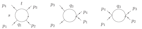
Figure 2: Kinematics of bubbles, one external mass triangle and no external mass box.

$$I_{2}^{n}\left(q_{3}^{\mu}\right) =\frac{1}{2}\left(p_{2}+p_{3}\right)^{\mu}I_{2}^{n},$$ (D.31)

$$I_{3}^{n}\left(q_{3}^{\mu}\right) =\frac{1}{t}I_{2}^{n}p_{2}^{\mu}-\left(I_{3}^{n}+\frac{1}{t}I_{2}^{n}\right)p_{3}^{\mu},$$ (D.32)

$$I_{4}^{n}(q_{1}^{\mu}) =-\frac{1}{2u}\left(tI_{4}^{n}(1234)-2I_{3}^{n}(s)+2I_{3}^{n}(t)\right)\left(p_{1}^{\mu}+p_{3}^{\mu}\right)+\frac{\left(p_{1}^{\mu}+p_{4}^{\mu}\right)}{2}I_{4}^{n}(1234),$$ (D.33)

$$I_{4}^{n}\left(\left(\mu^{2}+m^{2}\right)l_{1}^{\mu}\right) =-\frac{1}{2u}\left(tJ_{4}^{n}(1234)-2J_{3}^{n}(s)+2J_{3}^{n}(t)\right)\left(p_{1}^{\mu}+p_{3}^{\mu}\right)+\frac{\left(p_{1}^{\mu}+p_{4}^{\mu}\right)}{2}J_{4}^{n}(1234).$$ (D.34)

D.2 Reduction of extra-dimension scalar integrals

Here we give several formulas to calculate extra-dimension scalar integrals. Most of those results come from [3]. We can relate the extra scalar integral and the scalar integral in $n+2t$ dimensions:

$$\int\frac{d^{n}Q}{\left(2\pi\right)^{n}}\frac{(\mu^{2})^{t}}{D_{1}^{2}...D_{N}^{2}}\ =\ -\epsilon(1-\epsilon)....(t-1-\epsilon)(4\pi)^{t}\int\frac{d^{n+2t}Q}{\left(2\pi\right)^{n+2t}}\frac{1}{D_{1}^{2}...D_{N}^{2}}.$$ (D.35)

Using this formula we can calculate easily $J_{N}$ and $K_{N}$ function. Here we give some formula useful for this paper:

$$(-\epsilon)I_{4}^{n+2}\ =\ 0+O\left(\epsilon\right),$$ (D.36)

$$(-\epsilon)(1-\epsilon)I_{4}^{n+4}\ =\ -\frac{1}{6}+O\left(\epsilon\right).$$ (D.37)

We have:

$$J_{N}^{n}\ =\ m^{2}I_{N}^{n}+(-\epsilon)I_{N}^{n+2},$$ (D.38)

$$K_{N}^{n}\ =\ m^{4}I_{N}^{n}-2m^{2}\epsilon I_{N}^{n+2}+(-\epsilon)(1-\epsilon)I_{N}^{n+4}.$$ (D.39)

And the following relation holds between the $J_{4}$ and $I_{4}^{n+2}$ functions:

$$J_{4}^{n}(1234)\ =\ -\frac{st}{4u}I_{4}^{n}(1234)+\frac{s}{2u}I_{3}^{n}(s)+\frac{t}{2u}I_{3}^{n}(t)-\frac{1}{2}I_{4}^{n+2}(1234).$$ (D.40)

Appendix E Reduction of the pentagons and scalar hexagons

The method of reduction comes from [31]. The explicit reduction of massless scalar pentagon and massless scalar hexagon is in [7, 30, 32].

We note $I_{6}^{n}$ the hexagon in $n$ dimensions and $I_{5}^{n}\left(s_{ij}\right)$ the n-dimensional one-mass scalar pentagon. This pentagon is obtain by removing the propagator, of the scalar hexagon, between the external momentum $p_{i}$ and $p_{j}$. We note ${S_{6}}_{ij}$ the kinematical matrix of the hexagon and ${S_{5}}_{ij}$ the kinematical matrix of the pentagon.

According to [30, 31], the exact reduction of the hexagon is:

$$I_{6}^{n}\ =\ \sum_{k,l=1}^{6}{S_{6}}_{kl}^{-1}I_{5}^{n}\left(s_{l\ l+1}\right),$$ (E.41)

where the kinematical matrix is:

$${S^{6}}_{kl}=\begin{pmatrix}0&0&s_{23}&s_{234}&s_{16}&0\\ 0&0&0&s_{34}&s_{345}&s_{12}\\ s_{23}&0&0&0&s_{45}&s_{456}\\ s_{234}&s_{34}&0&0&0&s_{56}\\ s_{16}&s_{345}&s_{45}&0&0&0\\ 0&s_{12}&s_{456}&s_{56}&0&0\end{pmatrix}-2m^{2}\begin{pmatrix}1&1&1&1&1&1\\ 1&1&1&1&1&1\\ 1&1&1&1&1&1\\ 1&1&1&1&1&1\\ 1&1&1&1&1&1\\ 1&1&1&1&1&1\end{pmatrix}.$$ (E.42)

The reduction, in the leading order in $\epsilon$, of the pentagon is:

$$I_{5}^{n}(s)=\sum_{k,l=1}^{5}{S_{5,s}}_{kl}^{-1}I_{4}^{n}\left(s,s_{l\ l+1}\right)+O\left(\epsilon\right).$$ (E.43)

Where $I_{4}^{n}\left(s,s_{l\ l+1}\right)$ is the four-point scalar integral, obtain by removing the propagateur between the legs with the momentum $p_{l}$ and $p_{l+1}$ of the pentagon $I_{5}^{n}(s)$. The kinematical matrix for the pentagon $I_{5}(s_{12})$ is:

$${S_{5,s_{12}}}_{kl}=\begin{pmatrix}0&0&s_{34}&s_{345}&s_{12}\\ 0&0&0&s_{45}&s_{456}\\ s_{34}&0&0&0&s_{56}\\ s_{345}&s_{45}&0&0&0\\ s_{12}&s_{456}&s_{56}&0&0\end{pmatrix}-2m^{2}\begin{pmatrix}1&1&1&1&1\\ 1&1&1&1&1\\ 1&1&1&1&1\\ 1&1&1&1&1\\ 1&1&1&1&1\end{pmatrix}.$$ (E.44)

For another pentagon, we permute the labels. The hexagons and pentagons have no infrared divergences. We keep only the ”finite parts” of box functions. This part is usually called $F_{i}$, where the subscripts $i$ represents the number of external legs. We found those definitions in [7].

Appendix F Computation of the on-shell trees using in the paper

F.1 On-shell trees with two positive-helicity or two negative-helicity photons

Proposition 1:
Consider two positive-helicity photons with the momentum $p_{1}$ and $p_{2}$, join and connect them by an on-shell propagator, therefore we have:

$$\frac{\langle Rq_{1}1\rangle}{\langle R1\rangle}\frac{\langle Rq_{2}2\rangle}{\langle R2\rangle}=-\left(\mu^{2}+m^{2}\right)\frac{[12]}{\langle 12\rangle}.$$ (F.45)

In the case of two negative-helicity photons, we have:

$$\frac{[Rq_{1}1]}{[1R]}\frac{[Rq_{2}2]}{[2R]}=-\left(\mu^{2}+m^{2}\right)\frac{\langle 12\rangle}{[12]}.$$ (F.46)

Proof : We assume to have two photons with a positive helicity. We note $q_{0}=q_{1}-p_{1}$. And all propagators are on-shell, therefore $2(p_{1}.q_{0})=2(p_{2}.q_{2})=0$. Using this trick the amplitude is spelt:

$$\displaystyle\frac{\langle Rq_{1}1\rangle}{\langle R1\rangle}\frac{\langle Rq_{2}2\rangle}{\langle R2\rangle} =\displaystyle\frac{\langle Rq_{0}12q_{2}R\rangle}{\langle R1\rangle\langle R2\rangle\langle 12\rangle}=\displaystyle\frac{2(p_{2}.q_{2})\langle Rq_{0}1R\rangle-2(p_{1}.q_{0})\langle Rq_{2}2R\rangle+\langle R1q_{0}q_{2}2R\rangle}{\langle R1\rangle\langle R2\rangle\langle 12\rangle}$$ (F.47)

$$\displaystyle=\frac{q_{1}^{2}\langle R12R\rangle}{\langle R1\rangle\langle R2\rangle\langle 12\rangle}=\frac{\left(\mu^{2}+m^{2}\right)\langle R12R\rangle}{\langle R1\rangle\langle R2\rangle\langle 12\rangle}=-\left(\mu^{2}+m^{2}\right)\frac{[12]}{\langle 12\rangle}.$$ (F.48)

There is the same demonstration with negative-helicities photons.

Proposition 2:
Consider a chain of two positive-helicity photons with the momentum $p_{1}$ and $p_{2}$ surround with two on-shell propagators, therefore, we have:

$$\sum_{\sigma(1,2)}\frac{\langle Rq_{1}1\rangle}{\langle R1\rangle}\frac{i}{D_{1}^{2}}\frac{\langle Rq_{2}2\rangle}{\langle R2\rangle}=-\left(\mu^{2}+m^{2}\right)\frac{[12]}{\langle 12\rangle}\sum_{\sigma(1,2)}\frac{i}{D_{1}^{2}}.$$ (F.49)

If we have two negative-helicity photons, the chain is:

$$\sum_{\sigma(1,2)}\frac{[Rq_{1}1]}{[1R]}\frac{i}{D_{1}^{2}}\frac{[Rq_{2}2]}{[2R]}=-\left(\mu^{2}+m^{2}\right)\frac{\langle 12\rangle}{[12]}\sum_{\sigma(1,2)}\frac{i}{D_{1}^{2}}.$$ (F.50)

If the joined propagator is put on-shell therefore we find formula $\left(\ref{arbre1++},\ref{arbre1--}\right)$.

Proof :

$$\displaystyle\sum_{\sigma(1,2)}\frac{\langle Rq_{1}1\rangle}{\langle R1\rangle}\frac{i}{D_{1}^{2}}\frac{\langle Rq_{2}2\rangle}{\langle R2\rangle} =\displaystyle\sum_{\sigma(1,2)}\frac{i}{\langle R1\rangle\langle R2\rangle\langle 12\rangle}\frac{\langle Rq_{0}12q_{2}R\rangle}{D_{1}^{2}}$$ (F.51)

$$=\displaystyle\sum_{\sigma(1,2)}\frac{i}{\langle R1\rangle\langle R2\rangle\langle 12\rangle}\frac{2(p_{2}.q_{2})\langle Rq_{0}1R\rangle-2(p_{1}.q_{0})\langle Rq_{2}2R\rangle+\langle R1q_{0}q_{2}2R\rangle}{D_{1}^{2}}$$ (F.52)

$$=\displaystyle\sum_{\sigma(1,2)}\frac{i}{\langle R1\rangle\langle R2\rangle\langle 12\rangle}\frac{\left(D_{2}^{2}-D_{1}^{2}\right)\langle Rq_{0}1R\rangle-\left(D_{1}^{2}-D_{4}^{2}\right)\langle Rq_{2}2R\rangle+q_{1}^{2}\langle R12R\rangle}{D_{1}^{2}}$$ (F.53)

$$=\displaystyle\sum_{\sigma(1,2)}\frac{i}{\langle R1\rangle\langle R2\rangle\langle 12\rangle}\frac{\left(\mu^{2}+m^{2}\right)\langle R12R\rangle}{D_{1}^{2}}$$ (F.54)

$$=\displaystyle-\left(\mu^{2}+m^{2}\right)\frac{[12]}{\langle 12\rangle}\sum_{\sigma(1,2)}\frac{i}{D_{1}^{2}}.$$ (F.55)

Most of the reduction come from the permutation. For photons with a negative helicity, the proof is the same.

F.2 On-shell trees with one positive-helicity photon and one negative-helicity photon

Proposition 3:
Consider a diagram with a scalar line. On this scalar line with have first a chain with one on-shell negative-helicity photon and one on-shell positive-helicity photon. We assume that the momentum of negative-helicity photon (respectively positive-helicity photon) is: $p_{1}$ (respectively $p_{2}$). Moreover we assume that a third on-shell photon, with the momentum $p_{3}$, is ingoing in the scalar line just after this chain (fig. 3). The propagators around the chain are on-shell $D_{0}^{2}=0$ and $D_{2}^{2}=0$. The amplitude of this diagram is:

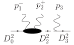
Figure 3: Chain composed with two photons, with two different helicity, following with one photon.

$$\displaystyle\frac{[r2]\langle R1\rangle}{2\langle R2\rangle[1r]}+\sum_{\sigma(1,2)}\frac{[rq_{1}1]}{[1r]}\frac{i}{D_{1}^{2}}\frac{\langle Rq_{2}2\rangle}{\langle R2\rangle}= \displaystyle-\frac{i}{\langle 231\rangle}\left(\frac{\langle 1q_{2}232\rangle-D_{3}^{2}\langle 1q_{2}2\rangle+\left(\mu^{2}+m^{2}\right)[231]}{D_{1}^{2}}\right)$$

$$-\frac{i}{\langle 231\rangle}\left(\frac{-D_{3}^{2}\langle 1q_{2}2\rangle+\langle 1q_{2}312\rangle+\left(\mu^{2}+m^{2}\right)[231]}{{D_{1}^{{}^{\prime}}}^{2}}\right).$$ (F.56)

Proof : We choose $|R\rangle=|1\rangle$ and $|r\rangle=|2\rangle$. The computation gives us:

$$\displaystyle\sum_{\sigma(1,2)}\frac{[rq_{1}1]}{[1r]}\frac{i}{D_{1}^{2}}\frac{\langle Rq_{2}2\rangle}{\langle R2\rangle}=-\frac{i\langle 1q_{2}2\rangle^{2}}{s_{12}}\sum_{\sigma(1,2)}\frac{1}{D_{1}^{2}}=\displaystyle-\frac{i}{s_{12}\langle 231\rangle}\left(\frac{\langle 1q_{2}231q_{2}2\rangle}{D_{1}^{2}}+\frac{\langle 1q_{2}231q_{2}2\rangle}{{D_{1}^{{}^{\prime}}}^{2}}\right)$$ (F.57)

$$= \displaystyle-\frac{i}{s_{12}\langle 231\rangle}\left(\frac{2(p_{1}.q_{2})\langle 1q_{2}232\rangle-2(p_{3}.q_{2})\langle 1q_{2}212\rangle+2(p_{2}.q_{2})\langle 1q_{2}312\rangle-q_{2}^{2}\langle 12312\rangle}{D_{1}^{2}}\right)$$

$$\displaystyle-\frac{i}{s_{12}\langle 231\rangle}\left(\frac{2(p_{1}.q_{2})\langle 1q_{2}232\rangle-2(p_{3}.q_{2})\langle 1q_{2}212\rangle+2(p_{2}.q_{2})\langle 1q_{2}312\rangle-q_{2}^{2}\langle 12312\rangle}{{D_{1}^{{}^{\prime}}}^{2}}\right)$$ (F.58)

$$= \displaystyle-\frac{i}{\langle 231\rangle}\left(\frac{\langle 1q_{2}232\rangle-D_{3}^{2}\langle 1q_{2}2\rangle+\left(\mu^{2}+m^{2}\right)[231]}{D_{1}^{2}}\right)-\frac{i}{\langle 231\rangle}\left(\frac{-D_{3}^{2}\langle 1q_{2}2\rangle+\langle 1q_{2}312\rangle+\left(\mu^{2}+m^{2}\right)[231]}{{D_{1}^{{}^{\prime}}}^{2}}\right).$$ (F.59)

Appendix G Four-cut technique for $A_{4}^{scalar}(-+++)$

In this appendix, we want to prove that, the integral $\left(\ref{M-+++1scamasse4cuts}\right)$ could be calculate without integration formulas, like $\left(\ref{annexeintegrationI4}\right)$. We use just the four on-shell conditions. We want to calculate the tensor integral:

$$(e\sqrt{2})^{4}\sum_{\sigma(2,3,4)}\frac{[34]}{\langle 34\rangle\langle 231\rangle}\int d^{n}Q\langle 1q_{2}232\rangle\left(\mu^{2}+m^{2}\right)\delta\left(D_{1}^{2}\right)\delta\left(D_{2}^{2}\right)\delta\left(D_{3}^{2}\right)\delta\left(D_{4}^{2}\right)$$ (G.60)

corresponding to the graph: .

The four-cut technique [15, 16, 17] says that the integrals $\left(\ref{LLL}\right)$ is:

$$(e\sqrt{2})^{4}\sum_{\sigma(2,3,4)}\frac{[34]}{\langle 34\rangle\langle 231\rangle}\frac{1}{2}\sum_{i}\langle 1{q_{2}}_{i}232\rangle\textrm{Disc}_{4}\int d^{n}Q\frac{\mu^{2}+m^{2}}{D_{1}^{2}D_{2}^{2}D_{3}^{2}D_{4}^{2}}$$ (G.61)

$$=\ (e\sqrt{2})^{4}\sum_{\sigma(2,3,4)}\frac{[34]}{\langle 34\rangle\langle 231\rangle}\frac{1}{2}\langle 1\sum_{i}{q_{2}}_{i}232\rangle\textrm{Disc}_{4}\int d^{n}Q\frac{\mu^{2}+m^{2}}{D_{1}^{2}D_{2}^{2}D_{3}^{2}D_{4}^{2}},$$ (G.62)

where ${q_{2}}_{i}$ are the solutions of:

$$D_{1}^{2} =0\ \Leftrightarrow\ \left(q_{2}-p_{2}\right)^{2}-\left(m^{2}+\mu^{2}\right)=0$$ (G.63)

$$D_{2}^{2} =0\ \Leftrightarrow\ q_{2}^{2}-\left(m^{2}+\mu^{2}\right)=0$$ (G.64)

$$D_{3}^{2} =0\ \Leftrightarrow\ \left(q_{2}+p_{3}\right)^{2}-\left(m^{2}+\mu^{2}\right)=0$$ (G.65)

$$D_{4}^{2} =0\ \Leftrightarrow\ \left(q_{2}+p_{3}+p_{4}\right)^{2}-\left(m^{2}+\mu^{2}\right)=0.$$ (G.66)

To solve this system of equations, we choose a basis of the four-dimension Minkowski space: $B=\left\{p_{2}^{\mu},p_{3}^{\mu},\langle 2\gamma^{\mu}3\rangle,\langle 3\gamma^{\mu}2\rangle\right\}$. In our case, ${q_{2}^{\mu}}_{i}$ is a four-dimension vector, therefore, we can project it on the base $B$:

$${q_{2}^{\mu}}_{i}\ =\ a_{i}\ p_{2}^{\mu}+b_{i}\ p_{3}^{\mu}+\frac{c_{i}}{2}\langle 2\gamma^{\mu}3\rangle+\frac{d_{i}}{2}\langle 3\gamma^{\mu}2\rangle.$$ (G.67)

So to know the vector ${q_{2}^{\mu}}_{i}$, we have to calculate, the four coefficients $a_{i},b_{i},c_{i}$ and $d_{i}$. The conditions $\left(\ref{equation1}\right)$ and $\left(\ref{equation2}\right)$ impose:

$$\left({q_{2}}_{i}-p_{2}\right)^{2}=m^{2}+\mu^{2}\Leftrightarrow 2\left(p_{2}.{q_{2}}_{i}\right)=0\Leftrightarrow b_{i}=0.$$ (G.68)

The conditions $\left(\ref{equation2}\right)$ and $\left(\ref{equation3}\right)$ impose:

$$\left({q_{2}}_{i}+p_{3}\right)^{2}=m^{2}+\mu^{2}\Leftrightarrow 2\left(p_{2}.{q_{2}}_{i}\right)=0\Leftrightarrow a_{i}=0.$$ (G.69)

The second condition $\left(\ref{equation2}\right)$ imposes:

$${q_{2}}_{i}^{2}=m^{2}+\mu^{2}\Leftrightarrow c_{i}d_{i}=-\frac{m^{2}+\mu^{2}}{s_{23}}.$$ (G.70)

And finally the two conditions $\left(\ref{equation3}\right)$ and $\left(\ref{equation4}\right)$ impose:

$$\left({q_{2}}_{i}+p_{3}+p_{4}\right)^{2}=m^{2}+\mu^{2}\Leftrightarrow c_{i}\langle 243\rangle+d_{i}\langle 342\rangle=-s_{34}.$$ (G.71)

So we have $a_{i}=b_{i}=0$ and the two equations $\left(\ref{condition1},\ref{condition2}\right)$ gives us $c_{i}$ and $d_{i}$. ${q_{2}}_{i}$ is totally define. Now we insert the decomposition $\left(\ref{decompositionq}\right)$ in the equation $\left(\ref{LLL1}\right)$ and we have:

$$\langle 1\sum_{i}{q_{2}}_{i}232\rangle=-t\langle 123\rangle\sum_{i}c_{i}=st\frac{\langle 123\rangle}{\langle 243\rangle}.$$ (G.72)

We input the last result in the integral $\left(\ref{LLL1}\right)$, and we obtain:

$$(e\sqrt{2})^{4}\sum_{\sigma(2,3,4)}\frac{[34]}{\langle 34\rangle\langle 231\rangle}\int d^{n}Q\langle 1q_{2}232\rangle\left(\mu^{2}+m^{2}\right)\delta\left(D_{1}^{2}\right)\delta\left(D_{2}^{2}\right)\delta\left(D_{3}^{2}\right)\delta\left(D_{4}^{2}\right)$$

$$=\ (e\sqrt{2})^{4}\sum_{\sigma(2,3,4)}\frac{[34][231]}{\langle 34\rangle\langle 231\rangle}\frac{ts}{2u}\textrm{Disc}_{4}J_{4}^{n}(1234).$$ (G.73)

This result is the result which we have obtain with the classical integration $\left(\ref{resultat-+++4cuts}\right)$.

References

- [1] R. Karplus and M. Neumann, Phys. Rev. 80 (1950) 380, 83 (1951) 776.
- [2] B. De Tollis, Nuovo Cim. 32 (1964) 757, 35 (1965) 1182.
- [3] Z.Bern and A.G.Morgan, Nucl. Phys. B 467 (1996) 479-509, [arXiv:hep-ph/9511336].
- [4] Z.Bern, A. De Freitas, L.Dixon, A.Ghinculov and H.L.Wong, JHEP 0111 (2001) 031, [arXiv:hep-ph/0109079].
- [5] T. Binoth, E. W. N. Glover, P. Marquard and J. J. van der Bij, JHEP 0205 (2002) 060, [arXiv:hep-ph/0202266].
- [6] A. Brandhuber, S. McNamara, B. J. Spence and G. Travaglini, JHEP 0510 (2005) 011, [arXiv:hep-th/0506068].
- [7] T. Binoth, J. P. Guillet, G. Heinrich and C. Schubert, Nucl. Phys. B 615 (2001) 385, [arXiv:hep-ph/0106243].
- [8] Z. Bern, L. J. Dixon and D. A. Kosower, Nucl. Phys. B 412 (1994) 751, [arXiv:hep-ph/9306240].
- [9] Z. Bern, L. Dixon and D. A. Kosower, Phys. Rev. Lett. 70 (1993) 2677-2680, [arXiv:hep-ph/9302280v1].
- [10] L. Dixon, [arXiv:hep-ph/9601359].
- [11] Z. Xu, D.H Zhang and L. Chang, Nucl. Phys. B 291 (1987) 392-428.
- [12] R.E. Cutkosky, J. Math. Phys 1 (1960) 429.
- [13] Z. Bern, L. Dixon and D.A. Kosower, Nucl.Phys. B 513 (1998) 3-86, [arXiv:hep-ph/9708239v1].
- [14] P. Mastrolia, Phys. Lett. B 644 (2007) 272, [arXiv:hep-th/0611091].
- [15] R. Britto, F. Cachazo and B. Feng, Nucl. Phys. B 725 (2005) 275, [arXiv:hep-th/0412103].
- [16] R. Britto, E. Buchbinder, F. Cachazo and B. Feng, Phys. Rev. D 72 (2005) 065012, [arXiv:hep-ph/0503132].
- [17] R. Britto, B. Feng and P. Mastrolia, Phys. Rev. D 73 (2006) 105004, [arXiv:hep-ph/0602178].
- [18] C. Anastasiou, R. Britto, B. Feng, Z. Kunszt and P. Mastrolia, Phys. Lett. B 645 (2007) 213, [arXiv:hep-ph/0612277].
- [19] Z. Bern, L. Dixon and D. A. Kosower, Ann. Rev. Nucl. Part. Sci. 46 (1996) 109-148, [arXiv:hep-ph/9602280v1].
- [20] G. Ossola, C.G. Papadopoulos and R. Pittau, JHEP 05 (2008) 004, [arXiv:0802.1876[hep-ph]].
- [21] R. Britto and B. Feng, Phys. Rev. D 75 (2007) 105006, [arXiv:hep-ph/0612089].
- [22] G. Ossola, C.G. Papadopoulos and R. Pittau, Nucl. Phys. B 763 (2007) 147-169, [arXiv:hep-ph/0609007].
- [23] D. Forde, Phys. Rev. D 75 (2007) 125019, [arXiv:hep-ph/0704.1835].
- [24] W. B. Kilgore, [arXiv:0711.5015].
- [25] S. Catani, M. H. Seymour and Z. Trocsanyi, Phys. Rev. D 55 (1997) 6819-6829, [arXiv:hep-ph/9610553].
- [26] A.G. Morgan, Phys. Lett. B 351 (1995) 249-256, [arXiv:hep-ph/9502230].
- [27] G. Ossola, C.G. Papadopoulos and R. Pittau, JHEP 07 (2007) 085, [arXiv:0704.1271 [hep-ph]].
- [28] Z. Nagy and D. E. Soper, Phys. Rev. D 74 (2006) 093006, [arXiv:hep-ph/0610028].
- [29] Z. Bern, L. Dixon, D.C. Dunbar and D.A. Kosower, Phys. Lett. B 394 (1997) 105-115, [arXiv:hep-th/9611127 v2]
- [30] Z. Bern, L. Dixon nd D.A. Kosower, Phys. Lett. B 302 (1993) 299-308; Erratum-ibid. B 318 (1993) 649, [arXiv:hep-ph/9212308v1].
- [31] T. Binoth, J. P. Guillet, G. Heinrich, E. Pilon and C. Schubert, JHEP 0510 (2005) 015, [arXiv:hep-ph/0504267].
- [32] T.Binoth, J.Ph. Guillet and G. Heinrich, Nucl. Phys. B 572 (2000) 361-386, [arXiv:hep-ph/9911342].
- [33] C.Bernicot and J.Ph. Guillet, JHEP 01 (2008) 059, [arXiv:0711.4713].