Multivariate Feller conditions in term structure models: Why do(n’t) we care?

Abstract

In this paper, the relevance of the Feller conditions in discrete time macro-finance term structure models is investigated. The Feller conditions are usually imposed on a continuous time multivariate square root process to ensure that the roots have nonnegative arguments. For a discrete time approximate model, the Feller conditions do not give this guarantee. Moreover, in a macro-finance context the restrictions imposed might be economically unappealing. At the same time, it has also been observed that even without the Feller conditions imposed, for a practically relevant term structure model, negative arguments rarely occur. Using models estimated on German data, we compare the yields implied by (approximate) analytic exponentially affine expressions to those obtained through Monte Carlo simulations of very high numbers of sample paths. It turns out that the differences are rarely statistically significant, whether the Feller conditions are imposed or not. Moreover, economically the differences are negligible, as they are always below one basis point.
Keywords: macro-finance models, affine term structure model, expected inflation, ex-ante real short rate, Monte Carlo simulations
JEL codes: E34, G13
Mathematics Subject Classification: 62P05, 62P20, 91B28

1 Introduction

This paper addresses the necessity of the so-called Feller conditions for an affine multivariate term structure model with time-varying volatility. Although already interesting from a theoretical point of view, the main motivation behind this study stems from sometimes unattractive implications of the Feller conditions in macro-finance models. A term structure model in general involves one or more driving factors, which are usually assumed unobservable. In the macro-finance models, the driving factors involve macro-economic variables, for instance the inflation rate. As these driving factors have a direct economic interpretation, the restrictions implied by the Feller conditions can be unappealing from an economic point of view. Consequently, most macro-finance term structure models assume a constant volatility for the driving factors, see for instance cv02, ap03, ab04, Dewachter, Lyrio and Maes (2004, 2006), fen05, brs05, dl06, htv06, wu06, and rw07. This however implies that interest rates are assumed symmetric, which means that either very low interest rates are predicted too often or very high interest rates not often enough. Especially for asset liability management purposes for pension funds, these characteristics can easily lead to wrong conclusions as the long duration of their liabilities makes them extremely sensitive to interest rate changes.

The Feller conditions serve several purposes in a continuous time affine term structure model with time-varying volatility. First of all, the dynamics of the factor processes involve square root terms and the conditions are sufficient to have the arguments of the square roots strictly positive. This in turn guarantees that the stochastic differential equations that describe the dynamics of the factor have a unique strong solution and that a closed form expression for the bond price can be obtained.

In practice, one often works with discrete time models, which, for instance, can be obtained by discretizing a continuous time model. For a discrete time model, existence of (strong) solutions is clearly not an issue and the Feller conditions play no role in this context. Moreover, the Feller conditions applied to a discretized model are useless to guarantee that the square roots always have nonnegative arguments. Indeed, the standard normally distributed errors, that are used as inputs in these discrete time models, imply that at each time instant there is a positive probability that one or more of the arguments of the square roots become negative, regardless whether the Feller conditions are satisfied or not. In spite of all this, it is not uncommon to impose the Feller conditions on discrete time models, as they serve as approximations of continuous time models.

In a two-dimensional setting with one volatility factor (denoted $v$), one of the Feller conditions imposes that for every point on the line $v=0$, the deterministic part of the process (the drift) is such that the volatility becomes positive again. Although it is clear that this condition is necessary in a univariate setting, its significance in a multivariate setting is not obvious as the interaction between the factors limits the part of the line $v=0$ that is actually approached. To illustrate this, Figure 1 shows a typical trajectory of a two-state factor process for a discrete time model with one volatility factor, and where the Feller conditions are not imposed. Although the line $v=0$ is crossed once, this happens in the area where the drift of the volatility process is positive, which would be impossible in a continuous time model. In other words, the fact that $v$ also assumes negative values is due to the discretization of the model, not because the Feller conditions are violated.

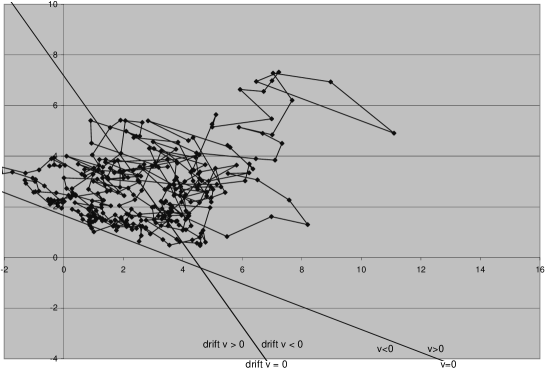
Figure 1: Example of a sample path of a discrete time ATSM for which the Feller conditions are not satisfied.

All this motivates a study that sheds some light on the necessity to impose the Feller conditions. If one assumes for a continuous time model that all volatilities are positive (which happens if the Feller conditions hold), there is an exponentially affine formula that expresses bond prices in terms of the state factor. The coefficients in this formula can be expressed in the model parameters. For a discrete time model, one can algebraically derive a similar expression, but again under the assumption that the square root factors are always positive. Since the latter does not hold (even when the Feller conditions are imposed), an exponential affine formula in discrete time has to be considered as yet another approximation for the bond price rather than an exact expression.

In order to investigate the accuracy of such an approximation, we compare them with an alternative method for validating bond prices, by making use of Monte Carlo simulations. This will be done for a multi-factor discrete time term structure model with expected inflation and the real short rate as factors. Such a model will be estimated using European data.

Since expected inflation is not observed, we use the Kalman filter combined with a likelihood approach to estimate the involved parameters. Estimation is performed for a number of cases, that will be referred to as models with independent volatilities, dependent volatilities and proportional volatilities. Each of these models will be estimated, with and without the Feller conditions imposed. In a pure latent variable model, it is usual to impose these conditions by assuming a canonical form, as in ds00. In such a canonical form the volatility factors are equal to some of the state factors. However, we cannot do this for a macro-finance model as ours, since none of the factors can be taken as a volatility factor a priori. Therefore we will extract explicit parameter restrictions from the Feller conditions for our non-latent variable model.

Having executed the estimation, we compare two consecutive approaches to validate bond prices. In the first one, we calculate the bond prices directly given the estimated parameters, using the Riccati equations (thereby ignoring the cut-off of volatility at zero). In the second approach, we perform a high number of Monte Carlo simulations of the trajectories of the factors, whereby volatility is restricted to be nonnegative. The mean of these simulations gives a second approximation of the bond price. Moreover, we can measure the approximation error with (sampled) confidence intervals. We will show that the differences between Monte Carlo results and the values obtained from the exponential affine formula are almost always negligible, both economically and statistically, whether the Feller conditions are imposed or not. From an economic point of view, the difference in implied yields between the two methods is hardly relevant, as it is at most one basis point. Statistically, the difference is only significantly different from zero for some maturities for the dependent and independent volatility models without Feller conditions. For the proportional volatility models, there is never a problem.

The rest of this paper is organized as follows. In Section 2 we review general and affine term structure models in continuous time, mainly with the aim to set the notation for the sections to follow. Moreover, we explicitly pin down the Feller conditions for a two-dimensional affine model, since the model is not given in canonical form. In Section 3 we discretize a continuous time model and show that the discretized model leads to the same expression for bond prices as a the discretized version of formula for bond prices in continuous time. In Section 4 we present and estimate our models. In Section 5 we use the estimated models of Section 4 to price bonds by Monte Carlo methods and compare the obtained results with those obtained by analytic methods. Finally in Section 6 we summarize our findings and draw some conclusions.

2 Affine term structure models in continuous time

Although we propose an affine term structure model for discrete time, we first discuss continuous time models. The reason for this is that the mathematical theory for affine term structure models was initially developed for continuous time models [Duffie and KanDuffie and Kan1996], whence in this respect it is natural to regard the equations governing the discrete time model as discretizations of the continuous time equations. In particular the Feller conditions we are interested in apply to continuous time models only. In order to understand the necessity of this condition in discrete time, we first have to understand the reason why it should be imposed for continuous time and then we can check whether these reasons still apply after discretization. Furthermore, since the Feller conditions use continuous time parameters, exact knowledge of the correspondence between discrete and continuous time parameters is required in order to impose it on the discrete time model.

2.1 Short rate term structure models

Let us first concisely recall some general theory of short rate term structure models, see Hunt, musrut or brimer for details. The formulas below will be used in subsequent sections. We assume that all relevant expressions are well defined.

In a short rate term structure model the price $D_{t,T}$ of a zero-coupon bond at time $t$ maturing at $T$ is based on the dynamics of the short rate $r$ through the formula

$$D_{t,T}=\mbox{{E}}_{\mathbb{Q}}(\exp(-\int_{t}^{T}r_{s}ds)|\mathcal{F}_{t}),$$ (1)

with $\mathbb{Q}$ the risk-neutral measure and $(\mathcal{F}_{t})$ the underlying filtration.

Typically, in a short rate model one chooses $r$ to be a function of a (possibly multi-dimensional) process $X$ which satisfies a stochastic differential equation (SDE)

$$dX_{t}=\mu(t,X_{t})dt+\sigma(t,X_{t})dW^{\mathbb{Q}}_{t},$$

with $W^{\mathbb{Q}}$ a multivariate Brownian motion under the risk-neutral measure $\mathbb{Q}$ and one writes $r_{t}=r(X_{t})$.

Under rather general conditions there exists a strong solution $X$ to this equation which is Markov. In this case the bond-price can be written as $D_{t,T}=\mbox{{E}}_{\mathbb{Q}}(\exp(-\int_{t}^{T}r(X_{s})ds)|X_{t})=:F(t,X_{t})$ for some function $F$. If $F$ is smooth enough, then it solves the fundamental partial differential equation (PDE), also called term structure equation (see [Chapter 12]musrut or vas77, where the latter terminology was introduced)

$$\frac{\partial}{\partial t}F(t,x)+\mathcal{L}F(t,x)-r(x)F(t,x)=0,\quad F(T,x)=1,$$ (2)

with

$$\mathcal{L}=\sum_{i}\mu_{i}\frac{\partial}{\partial x_{i}}+\frac{1}{2}\sum_{i,j}(\sigma\sigma^{\top})_{ij}\frac{\partial^{2}}{\partial x_{i}\partial x_{j}},$$

the generator of $X$, where $\sigma^{\top}$ means the transpose of $\sigma$.

The physical measure $\mathbb{P}$ is equivalent to the risk-neutral measure $\mathbb{Q}$ and related via a density process $L$ by $\left.L_{t}=\frac{d\mathbb{P}}{d\mathbb{Q}}\right|_{\mathcal{F}_{t}}.$ The process $L$ can often be written as an exponential process $\mathcal{E}(Y\cdot W^{\mathbb{Q}})$ for some $Y$, i.e.

$$L_{t}=\exp(\int_{0}^{t}Y^{\top}_{s}dW^{\mathbb{Q}}_{s}-\frac{1}{2}\int_{0}^{t}Y_{s}^{\top}Y_{s}ds),$$ (3)

where $Y_{s}$ is usually called the market price of risk. According to Girsanov’s theorem $W^{\mathbb{P}}_{t}=W_{t}^{\mathbb{Q}}-\int_{0}^{t}Y_{s}ds$ is a $\mathbb{P}$-Brownian motion, see [Section 3.5]Karshr for details on absolutely continuous measure transformations. Using these relations one can write the SDE for $X$ under the physical measure $\mathbb{P}$:

$$dX_{t} =(\mu(t,X_{t})+\sigma(t,X_{t})Y_{t})dt+\sigma(t,X_{t})dW^{\mathbb{P}}_{t}.$$ (4)

2.2 Affine term structure models

Affine term structure models (ATSM’s) are examples of short rate models and were introduced by dk96. We will give an overview here and explicitly point out where the Feller conditions are needed.

In an ATSM the short rate $r$ is an affine function of $X$, i.e. $r=\delta_{0}+\delta^{\top}X$ for some $\delta_{0}\in\mathbb{R}$, $\delta\in\mathbb{R}^{n}$, and $X$ satisfies under $\mathbb{Q}$ an $n$-dimensional affine square root SDE

$$dX_{t}=(aX_{t}+b)dt+\Sigma\sqrt{v(X_{t})}dW^{\mathbb{Q}}_{t}.$$ (5)

Here $W^{\mathbb{Q}}$ is an $n$-dimensional Brownian motion, $v(X_{t})$ is a diagonal matrix with on its diagonal the elements of the vector

$$\mbox{diag}[v(X_{t})]=\alpha+\beta X_{t},$$ (6)

with $\alpha\in\mathbb{R}^{n\times 1}$, $\beta\in\mathbb{R}^{n\times n}$ (so $v_{ii}(x)=\alpha_{i}+\beta_{i}x$, with $\beta_{i}$ the $i$-th row vector of $\beta$). We will call these elements volatility factors and we write $V_{t}:=v(X_{t})$ and $V_{i,t}:=v_{i}(X_{t})$. For brevity, we denote by $\sqrt{V_{t}}$ the matrix with on the diagonal the square roots $\sqrt{V_{i,t}\vee 0}$, that is the square root of the maximum of $V_{i,t}$ and 0. We will also use the notation $V_{t}\vee 0$ for the diagonal matrix with elements $V_{i,t}\vee 0$. Notice that $(\sqrt{V_{t}})^{2}=V_{t}\vee 0$.

Since the diffusion function $x\mapsto\Sigma\sqrt{v(x)}$ is not Lipschitz continuous for those $x$ for which $v(x)=0$, we cannot apply standard results to assure existence and uniqueness of a strong solution for (5), unless $V_{t}>0$ almost surely. The multivariate Feller conditions as given in dk96 and treated in section 2.3 are sufficient for this. Thus we have encountered the first reason to impose the Feller conditions.

In affine term structure models it is often desired that the process $X$ also satisfies an affine square root SDE under the physical measure $\mathbb{P}$, which considerably restricts the choice for the market price of risk $Y$. We only consider the so-called completely affine model, which means that we take $Y_{t}=\sqrt{V_{t}}\lambda$ with $\lambda\in\mathbb{R}^{n}$, and we refer to duf02 for other options. In this case the SDE (4) takes the form

$$dX_{t} =(aX_{t}+b+\Sigma(\sqrt{V_{t}})^{2}\lambda)dt+\Sigma\sqrt{V_{t}}dW^{\mathbb{P}}_{t}.$$ (7)

Under the condition that $V_{t}>0$ (elementwise on the diagonal), it holds that $(\sqrt{V_{t}})^{2}=V_{t}$ and Equation (7) reduces to

$$dX_{t} =(\widehat{a}X_{t}+\widehat{b})dt+\Sigma\sqrt{V_{t}}dW^{\mathbb{P}}_{t},$$ (8)

with $\widehat{a}=a+\Sigma(\beta\odot\lambda)$, $\widehat{b}=b+\Sigma(\alpha\odot\lambda)$. The affine structure of (8) is thus valid under the Feller conditions, which provides the second reason to have it imposed.

The third reason for imposing the Feller conditions is of more practical importance, as it concerns the closed-form expression for the bond price. Indeed, under these conditions it is possible to solve the term structure equation (2) by

$$F(t,x)=\exp(A(T-t)+B(T-t)^{\top}x),$$ (9)

for $t\in[0,T]$ and $x\in\mathcal{D}:=\{x\in\mathbb{R}^{n}:v_{i}(x)>0,\forall i\}$, where $A$ and $B$ satisfy the Riccati ordinary differential equations (ODE’s)

$$A^{\prime} =b^{\top}B+\frac{1}{2}\alpha^{\top}(\Sigma^{\top}B)^{\odot 2}-\delta_{0},\quad A(0)=0;$$ (10)

$$B^{\prime} =a^{\top}B+\frac{1}{2}\beta^{\top}(\Sigma^{\top}B)^{\odot 2}-\delta,\quad B(0)=0,$$ (11)

see dk96. However, if the bond price $D_{t,T}$ equals $F(t,X_{t})$, then it is necessary that $X_{t}\in\mathcal{D}$ almost surely, since the domain of $F$ is $[0,T]\times\mathcal{D}$. In other words, we need that $V_{i,t}>0$ almost surely, for all $i$ and $t$.

2.3 Multivariate Feller conditions in two dimensions

We will now treat the multivariate Feller conditions for positive volatility factors, as given in dk96.

Proposition 1 (dk96).

Let $X$ be a solution to the affine square root SDE (5). Then $X_{t}\in\mathcal{D},\forall t\geq 0$ holds almost surely under $\mathbb{Q}$ if the multivariate Feller conditions hold, that is for all $i$, $j$ we have

$$\beta_{i}\Sigma^{j} =0\mbox{ or $v_{i}=v_{j}+c$ for some $c\geq 0$},$$ (12)

$$\beta_{i}(ax+b) >\frac{1}{2}\beta_{i}\Sigma\Sigma^{\top}\beta_{i}^{\top}\mbox{ for all $x\in\partial\mathcal{D}^{i}$}.$$ (13)

where we write $\mathcal{D}:=\{x\in\mathbb{R}^{n}:v_{i}(x)>0,i=1,\ldots,n\}$, $\partial\mathcal{D}^{i}:=\{x\in\mathbb{R}^{n}:v_{i}(x)=0,v_{j}(x)\geq 0,\forall j\neq i\}$ and $\Sigma^{j}$ for the $j$-th column vector of $\Sigma$.

In a pure latent variable model the Feller conditions can be imposed by assuming a canonical form for SDE (5), as shown by ds00. In such a canonical form the volatility factors are equal to some of the state factors. However, we cannot do this for macro-finance models as requiring one of the factors to be the volatility factor is overly restrictive. Therefore we need to extract explicit parameter restrictions from the Feller conditions in order to impose it for a non-latent variable model. We will do this for dimension 2.

Let $X$ be a solution to the SDE (5) for $n=2$. We distinguish three cases: proportional (linear dependent) volatilities, linearly dependent but non-proportional volatilities and linearly independent volatilities. The first case is characterized by $v_{2}=kv_{1}$ for some $k\geq 0$, the second case corresponds to $v_{2}=kv_{1}+c$ with $k\geq 0$, $c>0$ and in the third case one has $\det\beta\not=0$. For the first and second case we take $k=1$, i.e. $k$ is absorbed in $\Sigma$, so that we can apply the above proposition. For future reference we also introduce $\gamma_{1}=(-\beta_{12},\beta_{11})$ and $\gamma_{2}=(\beta_{22},-\beta_{21})$, where the $\beta_{ij}$ are the elements of the matrix $\beta$.

Proportional volatilities:

Since we take $v_{2}=kv_{1}$ with $k=1$, condition (12) is automatically satisfied. Hence, for Proposition 1 to hold, we only have to impose (13). Note that $x\in\partial\mathcal{D}^{1}=\partial\mathcal{D}^{2}$ if and only if $x=-\frac{\alpha_{1}}{|\beta_{1}|^{2}}\beta_{1}^{\top}+y\gamma_{1}^{\top},\mbox{ for some }y\in\mathbb{R},$ where $|\beta_{1}|$ denotes the Euclidean norm of the vector $\beta_{1}$. Equation (13) for $i=1$ becomes $\beta_{1}(-\frac{\alpha_{1}}{|\beta_{1}|^{2}}a\beta_{1}^{\top}+ya\gamma_{1}^{\top}+b)>\frac{1}{2}\beta_{1}\Sigma\Sigma^{\top}\beta_{1}^{\top}\mbox{ for all }y\in\mathbb{R}.$ This reduces to the following set of conditions

$$-\frac{\alpha_{1}}{|\beta_{1}|^{2}}\beta_{1}a\beta_{1}^{\top}+\beta_{1}b >\frac{1}{2}\beta_{1}\Sigma\Sigma^{\top}\beta_{1}^{\top}$$ (14)

$$\beta_{1}a\gamma_{1}^{\top} =0.$$ (15)

Dependent but unproportional volatilities:

In this case $v_{2}=v_{1}+c$, with $c>0$. Then condition (12) is automatically satisfied for $i=2$, $j=1$, but for $i=1$, $j=2$ we have to impose the extra condition

$$\beta_{1}\Sigma^{2}=0.$$ (16)

Note that $\partial\mathcal{D}^{2}=\emptyset$, so for condition (13) we only have to consider the case $i=1$. The analysis is completely the same as for the case of proportional volatilities. Hence the conditions of Proposition 1 are equivalent to the set of conditions (14), (15) and (16).

Independent volatilities:

Suppose $\det\beta\not=0$, then $\beta^{-1}$ exists. Obviously neither $v_{2}=v_{1}+c$ nor $v_{1}=v_{2}+c$ holds true for some positive $c$, so for condition (12) to hold, we need to impose the restrictions

$$\beta_{1}\Sigma^{2}=0,$$ (17)

$$\beta_{2}\Sigma^{1}=0.$$ (18)

Note that $x\in\partial\mathcal{D}^{1}$, respectively $x\in\partial\mathcal{D}^{2}$, if and only if $\alpha+\beta x\in\{0\}\times\mathbb{R}_{\geq 0}$ respectively $\alpha+\beta x\in\mathbb{R}_{\geq 0}\times\{0\}$. Hence condition (13) is satisfied if and only if

$$\beta_{1}\left(a\beta^{-1}\left(\begin{pmatrix}0\\ w\end{pmatrix}-\alpha\right)+b\right) >\frac{1}{2}\beta_{1}\Sigma\Sigma^{\top}\beta_{1}^{\top},\quad\textnormal{for all }w\geq 0,$$ (19)

$$\beta_{2}\left(a\beta^{-1}\left(\begin{pmatrix}v\\ 0\end{pmatrix}-\alpha\right)+b\right) >\frac{1}{2}\beta_{2}\Sigma\Sigma^{\top}\beta_{2}^{\top},\quad\textnormal{for all }v\geq 0.$$ (20)

Since

$$\beta^{-1}=\frac{1}{\det\beta}\begin{pmatrix}\beta_{22}&-\beta_{12}\\ \\ -\beta_{21}&\beta_{11}\end{pmatrix}=\frac{1}{\det\beta}\begin{pmatrix}\gamma_{2}^{\top}&\gamma_{1}^{\top}\end{pmatrix},$$

we can reduce the restrictions (19) and (20) to

$$w\frac{\beta_{1}a\gamma_{1}^{\top}}{\det\beta}+\beta_{1}b-\beta_{1}a\beta^{-1}\alpha >\frac{1}{2}\beta_{1}\Sigma\Sigma^{\top}\beta_{1}^{\top},\quad\textnormal{for all }w\geq 0.$$

$$v\frac{\beta_{2}a\gamma_{2}^{\top}}{\det\beta}+\beta_{2}b-\beta_{2}a\beta^{-1}\alpha >\frac{1}{2}\beta_{2}\Sigma\Sigma^{\top}\beta_{2}^{\top},\quad\textnormal{for all }v\geq 0.$$

These hold true if and only if

$$\frac{\beta_{1}a\gamma_{1}^{\top}}{\det\beta} \geq 0$$ (21)

$$\frac{\beta_{2}a\gamma_{2}^{\top}}{\det\beta} \geq 0$$ (22)

$$\beta_{1}b-\beta_{1}a\beta^{-1}\alpha >\frac{1}{2}\beta_{1}\Sigma\Sigma^{\top}\beta_{1}^{\top}$$ (23)

$$\beta_{2}b-\beta_{2}a\beta^{-1}\alpha >\frac{1}{2}\beta_{2}\Sigma\Sigma^{\top}\beta_{2}^{\top}.$$ (24)

The first two are necessary since $v$ and $w$ can be chosen arbitrarily large, while the latter two follow by choosing $v=w=0$. In conclusion we can say that the requirements in Proposition 1 are met, if the conditions (17), (18) and (21)-(24) hold.

It is worth noting that $X_{t}\in\mathcal{D},\forall t\in[0,T]$ holds almost surely under $\mathbb{Q}$ if and only if it holds almost surely under $\mathbb{P}$, by the equivalence of $\mathbb{Q}$ and $\mathbb{P}$. Furthermore, $X$ solves (5) if and only if it solves (7), and under the conditions of the proposition it also solves (8). Hence one can rephrase the conditions of the proposition by using the parameters of (8) instead of those of (5), which gives the alternative to (13), but under (12) equivalent, condition

$$\beta_{i}(\widehat{a}x+\widehat{b})>\frac{1}{2}\beta_{i}\Sigma\Sigma^{\top}\beta_{i}^{\top}\mbox{ for all $x\in\partial\mathcal{D}^{i}$}.$$ (25)

Consequently, under $\mathbb{P}$ the Feller conditions are also fulfilled under restrictions (14) to (24), with $a$ and $b$ replaced by $\widehat{a}$ and $\widehat{b}$.

3 Affine term structure models in discrete time

In this section we take Equations (1), (5), (8), (9) as point of departure and transform it into their discrete time counterparts, using the Euler method [Kloeden and PlatenKloeden and Platen1999]. Next we investigate whether the resulting equations are consistent with each other and in which sense the Feller conditions are necessary in this respect.

In order not to complicate notation, we assume a discretization factor equal to one. We write $P_{n,t}$ for the bond price at time $t$ maturing at time $t+n$ (which corresponds to $D_{t,t+n})$ in continuous time). Basically, all continuous time formulas are translated to discrete-time by replacing integrals by sums and substituting $\Delta$ for $d$. By the properties of the Brownian motion we have $\Delta W^{\mathbb{Q}}_{t}=W^{\mathbb{Q}}_{t+1}-W^{\mathbb{Q}}_{t}\sim N(0,I)$ for each $t$, and all these increments are mutually independent. Therefore we write $\varepsilon^{\mathbb{Q}}_{t+1}$ instead of $dW_{t}^{\mathbb{Q}}$, with $\varepsilon^{\mathbb{Q}}_{t+1}$ i.i.d. standard normal variables under the risk neutral measure $\mathbb{Q}$. For the filtration we choose the natural filtration $\mathcal{F}_{t}=\sigma(\varepsilon^{\mathbb{Q}}_{k}:k=1,\ldots,t)$. We assume that $\mathbb{Q}$ and the physical measure $\mathbb{P}$ on $\mathcal{F}_{t}$ are related by $d\mathbb{P}=\widetilde{L}_{t}d\mathbb{Q}$, with $\widetilde{L}$ the discretized exponential process

$$\widetilde{L}_{t}=\exp(\sum_{k=0}^{t-1}\lambda^{\top}\sqrt{V_{k}}\varepsilon^{\mathbb{Q}}_{k+1}-\frac{1}{2}\sum_{k=0}^{t-1}\lambda^{\top}(V_{k}\vee 0)\lambda).$$

In the continuous time case, $W^{\mathbb{P}}$ defined by $dW^{\mathbb{P}}=dW^{\mathbb{Q}}_{t}-\sqrt{V_{t}}\lambda dt$ is a Brownian motion under $\mathbb{P}$ according to Girsanov’s theorem. Analogously, in discrete time, one can show that the $\varepsilon^{\mathbb{P}}_{t}$ defined by $\varepsilon^{\mathbb{P}}_{t+1}=\varepsilon^{\mathbb{Q}}_{t+1}-\sqrt{V_{t}}\lambda$ are i.i.d. standard normal variables under $\mathbb{P}$. So, we replace $dW^{\mathbb{P}}$ in (8) with $\varepsilon^{\mathbb{P}}$.

Application of the above substitutions enables us to transform the continuous time model into a discrete time model. The two stochastic differential equations (5) and (8) under $\mathbb{Q}$ and $\mathbb{P}$ respectively, transform into

$$X_{t+1} =(I+a)X_{t}+b+\Sigma\sqrt{V_{t}}\varepsilon^{\mathbb{Q}}_{t+1}$$ (26)

$$X_{t+1} =(I+\widehat{a})X_{t}+\widehat{b}+\Sigma\sqrt{V_{t}}\varepsilon^{\mathbb{P}}_{t+1}.$$ (27)

The bond price formula (1) becomes

$$P_{n,t} =\mbox{{E}}_{\mathbb{Q}}(\exp(-\sum_{k=0}^{n-1}r_{t+k})|\mathcal{F}_{t}).$$ (28)

Finally, the closed form expression (9) for the bond price in continuous time corresponds to $\widetilde{F}(n,x)=\exp(A_{n}+B_{n}^{\top}x)$ in discrete time, with $n=T-t$ and $A_{n}$ and $B_{n}$ the Euler discretizations of the solutions of the ODE’s (10) and (11). The latter means that $A_{n}$ and $B_{n}$ satisfy the Riccati recursions

$$A_{n+1} =A_{n}+b^{\top}B_{n}+\frac{1}{2}\alpha^{\top}(\Sigma^{\top}B_{n})^{\odot 2}-\delta_{0},\qquad A_{0}=0;$$ (29)

$$B_{n+1} =(I+a)^{\top}B_{n}+\frac{1}{2}\beta^{\top}(\Sigma^{\top}B_{n})^{\odot 2}-\delta,\qquad B_{0}=0,$$ (30)

which are equivalent to

$$A_{n+1} =A_{n}+(\widehat{b}-\Sigma(\alpha\odot\lambda))^{\top}B_{n}+\frac{1}{2}\alpha^{\top}(\Sigma^{\top}B_{n})^{\odot 2}-\delta_{0},\quad A_{0} =0;$$ (31)

$$B_{n+1} =(I+\widehat{a}-\Sigma(\beta\odot\lambda))^{\top}B_{n}+\frac{1}{2}\beta^{\top}(\Sigma^{\top}B_{n})^{\odot 2}-\delta,\quad B_{0} =0.$$ (32)

Now that we have derived the discrete time equations, it is important to note that it is impossible to prevent the volatility factors $V_{t,i}$ from becoming negative, since the noise variables are normally distributed. So in this respect it is useless to impose the Feller conditions. Does the possibility of negative volatility factors lead to any consistency problems for our discrete time model? We saw that in continuous time there were three reasons to have positive volatility factors. The first reason concerned existence and uniqueness of a strong solution for the SDE, which is not an issue in discrete time. The second reason was for writing $(\sqrt{V_{t}})^{2}$ as $V_{t}$, which enabled us to write (7) as (8), an affine square root SDE under the physical measure. Since in discrete time $V_{t}$ can always become negative, in this case it does not hold true that $(\sqrt{V_{t}})^{2}=V_{t}$, which implies that the dynamics of $X$ given by (26) and (27) are not consistent with each other. Recalling the definition of $\varepsilon^{\mathbb{P}}$, we see that there are two possibilities to solve this problem, either we keep (26) and replace (27) by

$$X_{t+1} =(I+a)X_{t}+b+\Sigma(V_{t}\vee 0)\lambda+\Sigma\sqrt{V_{t}}\varepsilon^{\mathbb{P}}_{t+1},$$ (33)

or we keep (27) and replace (26) by

$$X_{t+1} =(I+\widehat{a})X_{t}+\widehat{b}-\Sigma(V_{t}\vee 0)\lambda+\Sigma\sqrt{V_{t}}\varepsilon^{\mathbb{Q}}_{t+1}.$$ (34)

We opt for the latter, because an attractive expression under the physical measure is preferable in view of estimation of the parameters.

The third reason why we needed positive volatility factors in continuous time was to solve the term structure equation (2) in order to obtain a closed form expression $F$ for the bond price. There is no discrete time analogue of a term structure equation. However, using induction and the properties of a log-normal variable, we can algebraically derive a closed form expression for the bond price in discrete time, and, just as in continuous time, we need positiveness of the volatility factors for this, see Proposition 2 below. Remarkable is that this leads to the same expression as $\widetilde{F}$, the discretization of the closed form expression $F$ in continuous time. This is summarized in Figure 2 in a commutative diagram.

Proposition 2.

Let $X$ satisfy (26). Then for $P_{n,t}$ given by (28) it holds that

$$P_{n,t}\geq\widetilde{F}(n,t)=\exp(A_{n}+B_{n}^{\top}X_{t}),$$ (35)

with equality iff $V_{t}\geq 0$ almost surely for all $t$. The scalars $A_{n}$ and vectors $B_{n}$ satisfy the Riccati recursions (29) and (30).

• We give a proof by induction. For $n=0$ it holds that $P_{n,t}=P_{0,t}=1$, so the statement holds true with $A_{0}=B_{0}=0$. Now suppose $P_{n-1,t}\geq\exp(A_{n-1}+B_{n-1}^{\top}X_{t})$ for all $t$ and for a certain $n\in\mathbb{N}$. We write

  $$P_{n,t}=\mbox{{E}}_{\mathbb{Q}}\left[\exp\left(\left.-\sum_{k=0}^{n-1}r_{t+k}\right)\right|\mathcal{F}_{t}\right]=\mbox{{E}}_{\mathbb{Q}}\left[P_{n-1,t+1}e^{-r_{t}}|\mathcal{F}_{t}\right],$$

  and use the induction hypothesis to get

  $$P_{n,t} \geq\mbox{{E}}_{\mathbb{Q}}[\exp(A_{n-1}+B_{n-1}^{\top}X_{t+1}-\delta_{0}-\delta^{\top}X_{t})|\mathcal{F}_{t}]$$

  $$=\mbox{{E}}_{\mathbb{Q}}[\exp(A_{n-1}+B_{n-1}^{\top}((I+a)X_{t}+b+\Sigma\sqrt{V_{t}}\varepsilon^{\mathbb{Q}}_{t+1})-\delta_{0}-\delta^{\top}X_{t})|\mathcal{F}_{t}]$$

  $$=\exp(A_{n-1}+B_{n-1}^{\top}b-\delta_{0}+((I+a)^{\top}B_{n-1}-\delta)^{\top}X_{t})\mbox{{E}}_{\mathbb{Q}}[\exp(B_{n-1}^{\top}\Sigma\sqrt{V_{t}}\varepsilon^{\mathbb{Q}}_{t+1})|\mathcal{F}_{t}]$$

  $$\geq\exp(A_{n-1}+B_{n-1}^{\top}b-\delta_{0}+((I+a)^{\top}B_{n-1}-\delta)^{\top}X_{t}+\frac{1}{2}B_{n-1}^{\top}\Sigma V_{t}\Sigma^{\top}B_{n-1})$$

  $$=\exp\bigg{(}\underbrace{A_{n-1}+B_{n-1}^{\top}b-\delta_{0}+\frac{1}{2}\alpha^{\top}(\Sigma^{\top}B_{n-1})^{\odot 2}}_{\displaystyle A_{n}}$$

  $$\qquad\qquad\qquad\qquad\qquad\qquad+\underbrace{((I+a)^{\top}B_{n-1}-\delta+\frac{1}{2}\beta^{\top}(\Sigma^{\top}B_{n-1})^{\odot 2}}_{\displaystyle B_{n}})^{\top}X_{t}\bigg{)},$$

  where we have used that (with $\ell=\Sigma^{\top}B_{n-1}$)

  $$\mbox{{E}}_{\mathbb{Q}}[\exp(\ell^{\top}\sqrt{V_{t}}\varepsilon^{\mathbb{Q}}_{t+1})|\mathcal{F}_{t}]=\exp(\frac{1}{2}\ell^{\top}(V_{t}\vee 0)\ell)\geq\exp(\frac{1}{2}\ell^{\top}V_{t}\ell)$$ (36)

  and

  $$\ell^{\top}V_{t}\ell =\ell^{\top}(\alpha\odot\ell)+\ell^{\top}(\beta X_{t}\odot\ell)=\alpha^{\top}(\ell\odot\ell)+(\beta X_{t})^{\top}(\ell\odot\ell)=\alpha^{\top}\ell^{\odot 2}+X_{t}^{\top}\beta^{\top}\ell^{\odot 2}$$

  $$=\alpha^{\top}\ell^{\odot 2}+(\beta^{\top}\ell^{\odot 2})^{\top}X_{t}.$$

  If $V_{t}\geq 0$ then the inequality in (36) is an equality. This proves the assertion. $\Box$

Figure 2: Commutative diagram for calculating the bond-price in discrete time

Of course, the probability that $V_{t}$ gets negative is positive for all $t$, so $P_{n,t}$ is not equal to $\widetilde{F}(n,X_{t})$. Note also that the above proposition is inapplicable for our model, as $X$ solves (34) instead of (26). However, from a heuristic point of view, if $V_{t}$ gets negative with very small probability, (34) and (26) are “almost” equivalent and the inequality in (36) is “almost” an equality. This suggests that $\widetilde{F}$ might be a good approximation for $P$.

A priori though, it is not clear whether a model with parameters that satisfy the Feller conditions yields a better approximation than a model without parameter restrictions, as we do not know how the Feller conditions affect the probability for negative $V_{t}$ in discrete time. In fact, in the introduction we already saw an example in discrete time in which the relative frequency of negative $V_{t}$ was rather small, without having the Feller conditions imposed.

In the remaining sections we implement and estimate the discrete time model for dimension 2 using real data and we investigate how well in this case $\widetilde{F}$ approximates $P$. This is done by comparing $\widetilde{F}$ with Monte Carlo computations for the bond price $P$, based on (28) and (34).

4 Implementation and estimation of the discrete time ATSM

In this section, we investigate a two-factor model with the ex-ante real short term rate and expected inflation as state variables, the nominal short rate being the sum of these two factors. The interaction between interest rates and inflation is important, for instance for pension funds, as most of them have the intention to give indexation, whereas index linked bonds are hardly available. For the Netherlands, another important motivation for modeling this link is that supervision is geared toward nominal guarantees.

4.1 Specification of the model

Let $X_{1,t}$ denote the ex-ante real short term rate at time $t$ and $X_{2,t}$ the expected inflation. We use our dynamic model for quarterly data, so time is measured in quarters. Consequently, $r_{t}$ as used in the pricing formulas for bonds, is given in ordinary fractions per time unit, in our case per quarter. For numerical and readability reasons however, we want to express $X$ in percentages per year. Therefore, we have $r_{t}=(X_{1,t}+X_{2,t})/400$.

With respect to inflation, we are primarily interested in the ex-ante expectation and not so much in past realizations. Let $\pi_{t+1}$ denote the inflation rate from $t$ to $t+1$ (also in percentages per year), and $X_{2,t}$ its ex-ante expectation at date $t$. The observed processes are the short nominal rate $r_{t}$ and $\pi_{t}$. Since the inflation rate exhibits a seasonal pattern, we also include a seasonal contribution $S_{t}$ in the model.

Apart from the dynamics of the state process $X$ as given in Equation (27), our model is described by the following equations, that relate the state variables to the observations.

$$r_{t} =(X_{1,t}+X_{2,t})/400$$ (37a)

$$\pi_{t+1} =X_{2,t}+S_{t+1}+\omega_{\pi}\sqrt{V_{2,t-1}}\xi_{\pi,t+1}$$ (37b)

$$S_{t+1} =-S_{t}-S_{t-1}-S_{t-2}+\omega_{s}\sqrt{V_{2,t-1}}\xi_{s,t+1},$$ (37c)

where $\xi_{\pi,t}$ and $\xi_{s,t}$ are standard normally distributed error terms, that are independent under the physical measure of $\varepsilon_{t}^{\mathbb{P}}$ (which is the error term in the equation for $X_{t}$).

The data we are using for estimation are the observed longer maturity yields (denoted $r_{n,t}$, measured in fractions per quarter). These are modeled by the exponential affine expression for the bondprice plus a measurement error, which is assumed to be independently identically distributed among maturities:

$$r_{n,t}:=-\left(A_{n}+B_{n}X_{t}\right)/n+\left(\nu_{0}+\nu_{1}\sqrt{V_{1,t-1}}+\nu_{2}\sqrt{V_{2,t-1}}\right)\xi_{n,t},$$ (38)

under the restrictions $\nu_{i}\geq 0$, and where $\xi_{n,t}\sim N(0,I)$.

Having fully specified the model, we turn to the estimation procedure. A complicating matter is that both factors are not observed. Therefore, the extended Kalman filter [HarveyHarvey1989] is used to estimate the models. In principle, all parameters can be estimated simultaneously. In practice however, a one-step procedure tends to lead to unrealistic expected inflation predictions as the best fit for the bond prices are not necessarily achieved for the most realistic expected inflation estimates. As an appropriate modeling of the time series dynamics of interest rates and inflation is considered more important than the lowest measurement error for bond prices, we prefer a two-step procedure. In the first step, the parameters for system (37) are estimated, combined with the dynamics (27) for $X_{t}$ and its volatility (6). In the second step, the system is augmented by the equations for the long-term yields (38), and we estimate $\lambda$ and $\nu$, using the Riccati recursions (31) and (32), conditional on the first-step parameters.

4.2 Estimation results

The models are estimated with quarterly German data over the sample period 1959 to 2007. In order to estimate the dynamics between interest rates and inflation correctly, a long sample period is preferred. On the other hand, prices of zero coupon bonds are only available for a relatively short sample period, especially for longer maturities. Therefore, an unbalanced panel was used, with the short rate and inflation data starting in the last quarter of 1959, 1, 2, 4, 7 and 10-year rates starting the third quarter of 1972, the 15 year rate from 1986:II, and the 30-year rate from 1996:I on.

Table 1: Estimation results without the Feller conditions imposed

	Proportional volatilities	Dependent volatilities	Independent volatilities
$\begin{array}[]{c}\left(-\widehat{a}^{-1}\widehat{b}\right)^{\top}\end{array}$	$\left[\begin{array}[]{cc}2.36&3.05\\ (2.9)&(4.5)\end{array}\right]$	$\left[\begin{array}[]{cc}2.39&3.03\\ (3.0)&(6.3)\end{array}\right]$	$\left[\begin{array}[]{cc}2.33&3.12\\ (2.0)&(5.2)\end{array}\right]$
$I+\widehat{a}$	$\left[\begin{array}[]{cc}0.926&0.087\\ (26.5)&(1.7)\\ -0.002&0.938\\ (0.1)&(24.0)\end{array}\right]$	$\left[\begin{array}[]{cc}0.948&0.111\\ (26.3)&(2.8)\\ -0.026&0.950\\ (0.9)&(25.5)\end{array}\right]$	$\left[\begin{array}[]{cc}0.946&0.102\\ (24.4)&(2.2)\\ -0.006&0.940\\ (0.2)&(24.3)\end{array}\right]$
$\begin{array}[]{c}\alpha^{\top}\end{array}$	$\left[\begin{array}[]{cc}-0.377&-0.377\\ (2.3)&(2.3)\end{array}\right]$	$\left[\begin{array}[]{cc}-0.373&-0.165\\ (12.2)&(1.4)\end{array}\right]$	$\left[\begin{array}[]{cc}-0.377&-0.081\\ (3.2)&(1.5)\end{array}\right]$
$\begin{array}[]{c}\beta\end{array}$	$\left[\begin{array}[]{cc}0.105&0.230\\ (2.3)&(2.9)\\ 0.105&0.230\\ (2.3)&(2.9)\end{array}\right]$	$\left[\begin{array}[]{cc}0.108&0.194\\ (4.7)&(10.4)\\ 0.108&0.194\\ (4.7)&(10.4)\end{array}\right]$	$\left[\begin{array}[]{cc}0.117&0.193\\ (2.9)&(3.3)\\ 0.015&0.091\\ (1.4)&(2.6)\end{array}\right]$
$\Sigma$	$\left[\begin{array}[]{cc}1&0\\ (-)&(-)\\ -0.257&0.639\\ (1.5)&(5.3)\end{array}\right]$	$\left[\begin{array}[]{cc}1&-0.260\\ (-)&(1.7)\\ 0.052&0.547\\ (0.5)&(4.2)\end{array}\right]$	$\left[\begin{array}[]{cc}1&-0.526\\ (-)&(3.0)\\ 0.041&1\\ (0.3)&(-)\end{array}\right]$
$\begin{array}[]{c}\lambda^{\top}\end{array}$	$\left[\begin{array}[]{cc}0.105&-0.129\\ (0.7)&(1.3)\end{array}\right]$	$\left[\begin{array}[]{cc}0.108&-0.136\\ (0.6)&(1.4)\end{array}\right]$	$\left[\begin{array}[]{cc}0.0524&-0.209\\ (0.3)&(1.1)\end{array}\right]$

Estimation sample 1959:IV - 2007:II

Absolute two-step consistent t-values in parenthesis.

Table 1 shows the estimation results for the models without the Feller conditions imposed. As only the conditional covariance matrix of the noise terms, which is given by $\Sigma(V_{t}\vee 0)\Sigma^{\top}$, is identifiable, we fix $\Sigma_{11}=1$ in all models, we choose $\beta_{1}=\beta_{2}$ in the proportional and dependent models, we take $\Sigma_{12}=0$ in the proportional model, and $\Sigma_{22}=1$ in the independent model.

The mean real short rate is about 2.4% per year, whereas the mean inflation rate is just over 3%, the values in the top row of Table 1. With respect to the interaction between the short real rate and expected inflation, the lagged response ($\widehat{a}$) is in accordance with economic theory. Higher expected inflation leads to higher real rates, whereas higher real rates depress future inflation. The latter effect is far from significant though. With respect to volatility ($\alpha$ and $\beta$), both higher real rates and higher expected inflation lead to significantly higher variances.

Table 2: Estimation results with Feller conditions imposed

	Proportional volatilities	Dependent volatilities	Independent volatilities
$\begin{array}[]{c}\left(-\widehat{a}^{-1}\widehat{b}\right)^{\top}\end{array}$	$\left[\begin{array}[]{cc}2.34&3.04\\ (2.4)&(4.3)\end{array}\right]$	$\left[\begin{array}[]{cc}2.36&3.04\\ (1.9)&(3.3)\end{array}\right]$	$\left[\begin{array}[]{cc}2.91&2.83\\ (2.4)&(3.8)\end{array}\right]$
$I+\widehat{a}$	$\left[\begin{array}[]{cc}0.924&0.083\\ (25.0)&(1.5)\\ 0.016&0.925\\ (0.9)&(25.0)\end{array}\right]$	$\left[\begin{array}[]{cc}0.933&0.061\\ (22.2)&(1.2)\\ 0.021&0.936\\ (1.1)&(28.7)\end{array}\right]$	$\left[\begin{array}[]{cc}0.974&-0.009\\ (52.4)&(0.4)\\ 0&0.958\\ (-)&(47.9)\end{array}\right]$
$\begin{array}[]{c}\alpha^{\top}\end{array}$	$\left[\begin{array}[]{cc}-0.412&-0.412\\ (2.3)&(2.3)\end{array}\right]$	$\left[\begin{array}[]{cc}-0.098&-0.062\\ (5.7)&(1.4)\end{array}\right]$	$\left[\begin{array}[]{cc}0.020&-0.108\\ (0.7)&(4.5)\end{array}\right]$
$\begin{array}[]{c}\beta\end{array}$	$\left[\begin{array}[]{cc}0.108&0.252\\ (2.2)&(2.9)\\ 0.108&0.252\\ (2.2)&(2.9)\end{array}\right]$	$\left[\begin{array}[]{cc}0.028&0.049\\ (1.5)&(1.6)\\ 0.028&0.049\\ (1.5)&(1.6)\end{array}\right]$	$\left[\begin{array}[]{cc}0.071&-0.044\\ (2.6)&(1.2)\\ 0&0.100\\ (-)&(5.7)\end{array}\right]$
$\Sigma$	$\left[\begin{array}[]{cc}1&0\\ (-)&(-)\\ -0.292&0.640\\ (1.8)&(5.6)\end{array}\right]$	$\left[\begin{array}[]{cc}1&-1.620\\ (-)&(3.1)\\ 1.116&0.915\\ (1.9)&(2.0)\end{array}\right]$	$\left[\begin{array}[]{cc}1&0.615\\ (-)&(3.4)\\ 0&1\\ (-)&(-)\end{array}\right]$
$\begin{array}[]{c}\lambda^{\top}\end{array}$	$\left[\begin{array}[]{cc}0.0050&-0.124\\ (0.0)&(1.1)\end{array}\right]$	$\left[\begin{array}[]{cc}-0.153&0.667\\ (1.3)&(1.6)\end{array}\right]$	$\left[\begin{array}[]{cc}-0.397&-0.125\\ (1.2)&(0.1)\end{array}\right]$

Estimation sample 1959:IV - 2007:II

Absolute two-step consistent t-values in parenthesis.

Table 2 shows the results for the models that are restricted to fulfill the Feller conditions. In the independent volatility model, initially obtained estimates for $\Sigma_{21},\beta_{21}$ and $\widehat{a}_{21}$ were practically zero. Therefore, a zero value was subsequently imposed to increase accuracy of the other parameters. In this model, higher inflation now has a negative (though not significant) impact ($\hat{a}_{12}$) on future short term interest rates, which is contrary to economic theory, whereas in the previous case when the Feller conditions were not imposed, we found for this coefficient a positive value. In the other models, the impact of inflation on lagged real rates ($\widehat{a}_{21}$) is now positive, which is also in contrast with economic theory.

5 Monte Carlo results

Figure 3 shows the approximation errors made by the analytical expressions, in terms of yields, for each of the six cases as presented in Tables 1 and 2. The Monte Carlo simulations are based one million sample paths (containing 200 quarters) for the state variables. The yields are computed assuming the initial state variables are at their equilibrium values, which were a real short rate of about 2.4% and expected inflation of just over 3%.

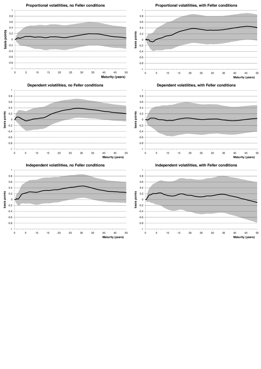
Figure 3: Mean and 99% confidence interval of the difference between simulated and analytical yields if starting state variables are in equilibrium

Ignoring the fact that volatilities are cut-off at zero does not seem to be important. Indeed, the 99% confidence band for the maximum approximation error in terms of yields stays within plus and minus one basis point (0.01%) for all models. It does not make much difference whether the Feller conditions are imposed (second column) or not (first column). Zero is almost always included in the confidence band, except for some maturities for the dependent and independent volatility models without Feller conditions imposed. For the proportional volatility model, there is never a problem, whether the Feller conditions are imposed or not.

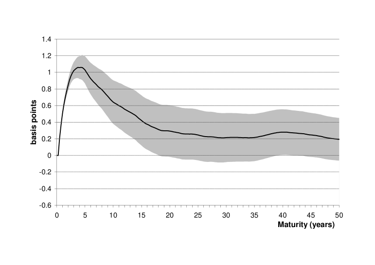
Figure 4: Mean and 99% confidence interval of the difference between simulated and analytical yields. Dependent volatility model without Feller conditions, starting from a volatility of zero.

It might be the case that these good approximations are due to the fact the approximation errors are calculated for the equilibrium yield curve. If the initial state variables imply a volatility closer to zero, ignoring the cut-off at $v=0$ might be more serious. Therefore, we also calculated the approximation errors for those state variables for which volatility was the lowest in the past. Figure 4 shows the worst result we found. Indeed, for maturities up to 15 years, the simulated yields are significantly higher than the analytical ones. The reason is that for the initial state variables, the volatility is cut-off at zero. As the state variables evolve according to (34), whereas the formulas underlying the formulas assume (26), systematic differences arise. Moreover, as the simulated yields are almost deterministic for short maturities, the confidence band is extremely small. In economic terms, the approximation error is still negligible though (at most one basis point).

Finally, as the Feller conditions do not guarantee positive volatilities in the discrete time model, imposing them does not preclude statistically significant approximation errors from arising either. Indeed for both the dependent and independent volatility models with Feller conditions we found starting conditions for which significant negative approximation errors for maturities up to 17 years occur. However, as the maximum magnitude of these errors is at most 0.5 basis point, the economic relevance is again negligible.

6 Conclusions

The Feller conditions are imposed on a continuous time multivariate square root process in order to have well defined strong solutions to the stochastic differential equations and to ensure that the roots have nonnegative arguments. For a discrete time approximate model, the Feller conditions loose part of their relevance. Existence of strong solutions is not an issue anymore and since the noise involves standard normal errors, there is always a positive probability that arguments of square roots become negative. Nevertheless, keeping in mind the idea that a discrete time model is an approximation of a continuous time model, it is natural to still impose the Feller conditions. On the other hand, it has also been observed that even without the Feller conditions imposed, for a practically relevant model, negative arguments rarely occur.

We have investigated the relevance of imposing the Feller conditions for a two-factor affine term structure model, where the factors (ex-ante real short term interest rate and expected inflation) are modelled as a square root process. As we want to allow volatilities to depend on both state variables, the models are not estimated in canonical form. Therefore we also explicitly presented the Feller conditions for square root models not in canonical form.

Three different models have been used, that have been referred to as models with proportional, dependent and independent volatilities, either with or without the Feller conditions on the parameters. The parameters of each of the underlying models have been estimated using quarterly German data. The restrictions involved in imposing the Feller conditions resulted in unappealing economic results. In the proportional and dependent volatility models, the restrictions imply a positive impact of interest rates on inflation, whereas in the independent volatility model, inflation now leads to lower interest rates. Both elements are contrary to the accepted economic theory.

For these six cases we have compared the resulting yields, that are either obtained by (approximate) analytic exponentially affine expressions or those obtained through Monte Carlo simulations of very high numbers of sample paths. It turned out that the approximation errors in analytical yields were rarely statistically significant, and never economically relevant, as they were always below one basis point. In particular a proportional volatility model without the Feller conditions imposed already gave very good results.

References

- [\citeauthoryearAng and BekaertAng and Bekaert2004] Ang, A. and K.G. Bekaert (2004), ‘The term structure of real rates and expected inflation’, CEPR Discussion Paper 4518.
- [\citeauthoryearAng and PiazzesiAng and Piazzesi2003] Ang, A. and M. Piazzesi (2003), ‘A no-arbitrage vector autoregression of term structure dynamics with macroeconomic and latent variables’, Journal of Monetary Economics 50(4), 745–787.
- [\citeauthoryearBackus, Foresi, and TelmerBackus et al.2001] Backus, D., S. Foresi, and C. Telmer (2001, 02), ‘Affine term structure models and the forward premium anomaly’, Journal of Finance 56(1), 279–304.
- [\citeauthoryearBernanke, Reinhart, and SackBernanke et al.2005] Bernanke, B., V. Reinhart, and B. Sack (2005), ‘Monetary policy alternatives at the zero bound: An empirical assessment’, Brookings Papers on Economic Activity, 2, 1–78.
- [\citeauthoryearBolderBolder2001] Bolder, D.J. (2001), ‘Affine term-structure models: Theory and implementation’, Working Paper 2001-15, Bank of Canada.
- [\citeauthoryearBrigo and MercurioBrigo and Mercurio2006] Brigo, D. and F. Mercurio (2006), Interest rate models—theory and practice (Second ed.), Springer Finance, Berlin: Springer-Verlag, With smile, inflation and credit.
- [\citeauthoryearCampbell and ViceiraCampbell and Viceira2002] Campbell, J.Y. and L.M. Viceira (2002), Strategic Asset Allocation, Clarendon Lectures in Economics: Oxford University Press.
- [\citeauthoryearChen and ScottChen and Scott2003] Chen, R.R. and L. Scott (2003), ‘Multi-factor Cox-Ingersoll-Ross models of the term structure: Estimates and tests from a Kalman filter model’, Journal of Real Estate Finance and Economics 27(2), 143–172.
- [\citeauthoryearDai, Le, and SingletonDai et al.2005] Dai, Q., A. Le, and K.J. Singleton (2005), ‘Discrete-time dynamic term structure models with generalized market prices of risk’, Manuscript, Stanford University.
- [\citeauthoryearDai and SingletonDai and Singleton2000] Dai, Q. and K.J. Singleton (2000), ‘Specification analysis of affine term structure models’, Journal of Finance 55(5), 1943–1978.
- [\citeauthoryearDe JongDe Jong2000] De Jong, F. (2000), ‘Time-series and cross-section information in affine term structure models’, Journal of Business and Economic Statistics, 18, 300–314.
- [\citeauthoryearDe RossiDe Rossi2006] De Rossi, G. (2006), ‘Unit roots and the estimation of multifactor Cox-Ingersoll-Ross models’, Manuscript, Cambridge University.
- [\citeauthoryearDewachter and LyrioDewachter and Lyrio2006] Dewachter, H. and M. Lyrio (2006), ‘Macro factors and the term structure of interest rates’, Journal of Money, Credit, and Banking 38(1), 119–140.
- [\citeauthoryearDewachter, Lyrio, and MaesDewachter et al.2004] Dewachter, H., M. Lyrio, and K. Maes (2004), ‘The effect of monetary unification on German bond markets’, European Financial Management 10(3), 487–509.
- [\citeauthoryearDewachter, Lyrio, and MaesDewachter et al.2006] Dewachter, H., M. Lyrio, and K. Maes (2006), ‘A joint model for the term structure of interest rates and the macroeconomy’, Journal of Applied Econometrics, 21, 439–462.
- [\citeauthoryearDuan and SimonatoDuan and Simonato1999] Duan, J.C. and J.G. Simonato (1999), ‘Evaluating an alternative risk preference in affine term structure models’, Review of Quantitative Finance and Accounting, 13, 111–135.
- [\citeauthoryearDuffeeDuffee2002] Duffee, G.R. (2002), ‘Term premia and interest rate forecasts in affine models’, Journal of Finance 57(1), 405–443.
- [\citeauthoryearDuffee and StantonDuffee and Stanton2004] Duffee, G.R. and R.H. Stanton (2004), ‘Estimation of dynamic term structure models’, Manuscript, Haas School of Business.
- [\citeauthoryearDuffie and KanDuffie and Kan1996] Duffie, D. and R. Kan (1996), ‘A yield-factor model of interest rates’, Mathematical Finance 6(4), 379–406.
- [\citeauthoryearFendelFendel2005] Fendel, R. (2005), ‘An affine three-factor model of the German term structure of interest rates with macroeconomic content’, Applied Financial Economics Letters 1(3), 151–156.
- [\citeauthoryearHarveyHarvey1989] Harvey, A.C. (1989), Forecasting, structural time series models and the Kalman filter. Cambridge University Press.
- [\citeauthoryearHördahl, Tristani, and VestinHördahl et al.2006] Hördahl, P., O. Tristani, and D. Vestin (2006), ‘A joint econometric model of macroeconomic and term-structure dynamics’, Journal of Econometrics 131(1-2), 405–444.
- [\citeauthoryearHunt and KennedyHunt and Kennedy2000] Hunt, P. and J. Kennedy (2000), Financial Derivatives in Theory and Practice. Wiley Series in Probability and Statistics.
- [\citeauthoryearKaratzas and ShreveKaratzas and Shreve1991] Karatzas, I. and S. Shreve (1991), Brownian Motion and Stochastic Calculus. Springer-Verlag.
- [\citeauthoryearKloeden and PlatenKloeden and Platen1999] Kloeden, P.E. and E. Platen (1999), Numerical Solution of Stochastic Differential Equations. Springer.
- [\citeauthoryearLundLund1997] Lund, J. (1997), ‘Econometric analysis of continuous-time arbitrage-free models of the term structure of interest rates’, Working Paper, Aarhus School of Business.
- [\citeauthoryearMusiela and RutkowskiMusiela and Rutkowski1997] Musiela, M. and M. Rutkowski (1997), Martingale methods in financial modelling, Volume 36 of Applications of Mathematics (New York), Berlin: Springer-Verlag.
- [\citeauthoryearRudebusch and WuRudebusch and Wu2007] Rudebusch, G.D. and T. Wu (2007), ‘Accounting for a shift in term structure behavior with no-arbitrage and macro-finance models’, Journal of Money, Credit, and Banking, forthcoming.
- [\citeauthoryearSpencerSpencer2004] Spencer, P. (2004), ‘Affine macroeconomic models of the term structure of interest rates: The US treasury market 1961-99’, Discussion Papers in Economics 2004/16, The University of York.
- [\citeauthoryearVasicekVasicek1977] Vasicek, O.A. (1977), ‘An equilibrium characterization of the term structure’, Journal of Financial Economics, 5, 177–188.
- [\citeauthoryearWuWu2006] Wu, T. (2006), ‘Macro factors and the affine term structure of interest rates’, Journal of Money, Credit, and Banking 38(7), 1847–1875.