On the Spectral Properties of Matrices Associated with Trend Filters

On the Spectral Properties of Matrices Associated with Trend Filters

Abstract

This paper is concerned with the spectral properties of matrices associated with linear filters for the estimation of the underlying trend of a time series. The interest lies in the fact that the eigenvectors can be interpreted as the latent components of any time series that the filter smooths through the corresponding eigenvalues. A difficulty arises because matrices associated with trend filters are finite approximations of Toeplitz operators and therefore very little is known about their eigenstructure, which also depends on the boundary conditions or, equivalently, on the filters for trend estimation at the end of the sample.

Assuming reflecting boundary conditions, we derive a time series decomposition in terms of periodic latent components and corresponding smoothing eigenvalues. This decomposition depends on the local polynomial regression estimator chosen for the interior. Otherwise, the eigenvalue distribution is derived with an approximation measured by the size of the perturbation that different boundary conditions apport to the eigenvalues of matrices belonging to algebras with known spectral properties, such as the Circulant or the Cosine. The analytical form of the eigenvectors is then derived with an approximation that involves the extremes only.

A further topic investigated in the paper concerns a strategy for a filter design in the time domain. Based on cut-off eigenvalues, new estimators are derived, that are less variable and almost equally biased as the original estimator, based on all the eigenvalues. Empirical examples illustrate the effectiveness of the method.

Keywords

Smoothing, Toeplitz matrices, Spectral analysis, Boundary conditions, Matrix algebras, Approximate asymmetric filters, Bias-Variance trade-off.

1 Introduction

The smoothing problem has a long and well established tradition in statistics and has a wide range of applications in time series analysis; see Anderson (1971, ch. 3), Kendall (1973), Kendall, Stuart and Ord (1983) and Cleveland and Loader (1996). In its simplest form, it aims at providing a measure of the underlying tendency from noisy observations, and takes the name of signal extraction in engineering, trend estimation in econometrics, and graduation in actuarial sciences. This paper is concerned with local polynomial regression methods, that developed as an extension of least squares regression and result in estimates that are linear combinations of the available information. These linear combinations are often termed filters and their analysis provides useful insight into what the method does.

The properties of linear filters are traditionally studied on different, complementary viewpoints. In the time domain, the analysis of the filter weights provides information on the amount of bias introduced and variance left in the input data from the smoothing procedure. In the frequency domain, the basic assumption is that a time series can be decomposed as a linear combination of trigonometric functions. The variability and the dependence relation among the variables are then evaluated in terms of the contribution of such components with respect to some frequency or periodicity, usually measured in radians.

An alternative approach consists of analysing the matrices associated with linear filters. Though smoothers have been introduced in a time series framework, with the works of Whittaker (1923) on spline smoothing and of Henderson (1916, 1924) on graduation by averages, they have been mainly analysed in the context of linear regression and in generalised additive models, following the approach of Buja, Hastie and Tibshirani (1989, section 2) and Hastie and Tibshirani (1990, section 3.7), based on the smoother matrices associated with linear estimators. In these references, the attention is concentrated on symmetric matrices that arise as the solutions of penalised least squares problems, such as the cubic smoothing spline estimators (see Whaba, 1990, and Green and Silverman, 1994). The spectral properties of smoother matrices are analysed and inferential procedures based on eigenvalues and eigenvectors are developed. The authors remark that eigenanalysis is no longer useful for non symmetric smoother matrices because of complex eigenvalues and eigenvectors and argue that the spectral analysis of a smoother matrix is closely related to the study of the transfer function of the associated linear filter for time series.

These two remarks motivated the present paper. In considering local polynomial regression methods for the estimation of the underlying trend of a time series, symmetry is in general lost and replaced by centrosymmetry. At the same way, the interpretation that can be ascribed to the eigenvalues and eigenvectors of time series smoothing matrices (let us suppose for the moment that we are capable to lead the problem to the real or to the symmetric case) provides useful information on the estimation method. In fact, the eigenvectors of matrices associated with local polynomial regression estimators can be interpreted as the latent components of any time series that the filter smooths through the corresponding eigenvalues. This interpretation allows a decomposition of a time series in periodic latent components that depend on the estimation method and opens the way to eigenvalue-based inferential procedures. Furthermore, it is possible to establish a formal connection between the spectrum of a smoothing matrices and the transfer function of the associated filter.

This paper analyses the spectral properties of matrices associated with trend filters. In referring to spectral properties in a time series setting, we shall distinguish between two accomplished theories: the spectral analysis of a linear filter, where the filter properties are studied in the frequency domain, and the spectral properties of the associated matrix, i.e. the study of its eigenvalues and eigenvectors. Both these techniques are related to the concept of spectrum, to be intended as a latent characteristic that cannot be directly observed. The spectral properties of linear filters have been widely investigated in time series analysis, where classical references are the books by Jenkins and Watts (1968), Priestley (1981), Bloomfield (2000). On the other hand, the spectral properties of the associated matrices have not been explored. One reason is certainly due to the lack of attention surrounding time series smoothing matrices. Another justification relies on the fact that the mathematics of these matrices is rather problematical. In fact, they can be interpreted as finite approximations of infinite symmetric banded Toeplitz operators. The latter have been extensively explored, but their finite counterparts subject to boundary conditions are much more difficult to analyse (see Böttcher and Grudsky, 2005; see also Gray, 2006). Established results hold for tridiagonal matrices, but when the span of the filter increases, the algebra becomes extremely complicated and, except for some cases, only approximate results can be obtained. The size of the approximation essentially depends on the boundary conditions on the finite matrix. Furthermore, the boundary conditions determine the asymmetric filters for the estimation of the trend at the extremes of the series. Specifically, two-sided symmetric filters cannot be applied since future (or past) observations are not available. It should be remarked that the estimates at the end of the sample are crucial in current analysis.

We derive approximate results on the eigenvalues and eigenvectors of matrices associated with trend filters by interpreting the latter as perturbations of matrices belonging to the circulant and to the reflecting algebras, for which eigenvalues and eigenvectors can be known exactly even in finite dimensions. The underlying hypothesis is that of a circular and of a reflecting process, respectively. The key result is a perturbation theorem that draws some conclusions on the distribution of the eigenvalues of the original smoothing matrices. We then relate the absolute eigenvalue distribution to the gain function of the corresponding symmetric filter. To illustrate these results, we consider a class of asymmetric filters that approximate a given symmetric estimator with a minimum mean square revision error strategy, subject to polynomial constraints. This class encompasses the local polynomial regression filters that automatically adapt at the boundaries and that under mild assumptions on the trend are unbiased estimators. Concerning the eigenvectors, we show that filters that are unbiased with respect to polynomial trends of order $p$ have $p+1$ eigenvectors that describe polynomial functions up to the degree $p$. The analytical form of the remaining eigenvectors is derived with an approximation which involves the extremes only. A further topic investigated in the paper concerns a strategy for a filter design in the time domain. Based on cut-off eigenvalues, it is possible to obtain new estimators that, in the interior, have less variance and almost equal bias than the original estimator. The effectiveness of this method is illustrated with empirical examples. We would like to remark that even if these results are derived in a time series setting, they apply to any non symmetric banded smoother matrix.

The paper is organised as follows. Section 2 reviews the derivation of linear smoothers for trend extraction, both in the interior and at the boundaries (section 2.1), providing examples that will be used for the applications of the methods developed later on in the paper. In section 3, time series smoothing matrices are introduced and their properties are illustrated. Section 4 contains the major results of the paper, i.e. the spectrum analysis of matrices associated with trend filters. Specifically, two sets of boundary conditions are are considered, circulant (section 4.2) and reflecting (section 4.3). Furthermore, we provide the interpretation of the eigenvectors as analytical periodic functions of the time. In section 5, a strategy for a filter design based on a selected number of latent components is derived, based on a suitably chosen cut-off eigenvalue. The bias-variance trade off between old and new estimators is evaluated (section 5.1) and the new filters are applied to real data (section 5.2). Section 6 summarises and comments on the results. Proofs and other technical details are given in section 7.

2 Local polynomial regression methods

Time series analysis is often based on additive models like

$$y_{t}=\mu_{t}+\epsilon_{t},t=1,\ldots,n,$$ (1)

where $y_{t}$ is the observed time series, $\mu_{t}$ is the trend component, also termed the signal, and $\epsilon_{t}$ is the noise, or irregular, component. The signal $\mu_{t}$ can be a random or deterministic smooth function of time whereas the most common assumption for the noise $\epsilon_{t}$ is that it follows a zero mean stochastic process, such as a White Noise or/and Gaussian. Let us assume that in (1) $\mu_{t}$ is an unknown deterministic function of time, so that $\mbox{E}(y_{t})=\mu_{t}$, and that equally spaced observations $y_{t+j},j=0,\pm 1,2,\ldots,h,$ are available in a neighbourhood of time $t$. Our interest lies in estimating the level of the trend at time $t$, $\mu_{t}$, using the available observations. If $\mu_{t}$ is differentiable, using the Taylor-series expansion it can be locally approximated by a polynomial of degree $p$ of the time distance, $j$, between $y_{t}$ and the neighbouring observations $y_{t+j}$. Hence, $\mu_{t+j}\approx m_{t+j}$, with

$$m_{t+j}=\beta_{0}+\beta_{1}j+\cdots+\beta_{p}j^{p},j=0,\pm 1,\ldots,\pm h.$$

The degree of the polynomial is crucial in determining the accuracy of the approximation. Another essential quantity is the size $h$ of the neighbourhood around time $t$; for $t=h+1,...,n-h+1$, the neighbourhood consists of $2h+1$ consecutive and regularly spaced time points at which observations $y_{t+j}$ are made. At the boundaries, asymmetric neighborhood will be considered. The parameter $h$ is the bandwidth, for which we assume $p\leq 2h$ throughout.

Replacing $\mu_{t+j}$ by its approximation gives the local polynomial model:

$$y_{t+j}=\sum_{k=0}^{p}\beta_{k}j^{k}+\epsilon_{t+j},\;\;\;j=0,\pm 1,\ldots,\pm h.$$ (2)

Assuming that $\epsilon_{t+j}\sim\mbox{NID}(0,\sigma^{2})$, then (2) is a linear Gaussian regression model with explanatory variables given by the powers of the time distance $j^{k},k=0,\ldots,p$ and unknown coefficients $\beta_{k}$, which are proportional to the $k$-th order derivatives of $\mu_{t}$. Working with the linear Gaussian approximating model, we are faced with the problem of estimating $m_{t}=\beta_{0}$, i.e. the value of the approximating polynomial for $j=0$, which is the intercept $\beta_{0}$ of the approximating polynomial.

The model (2) can be rewritten in matrix notation as follows:

$$\mathbf{y}=\mathbf{X}\mbox{\boldmath$\beta$}+\mbox{\boldmath$\epsilon$},\;\;\;\mbox{\boldmath$\epsilon$}\sim\mbox{N}(\mbox{\bf{0}},\sigma^{2}\mathbf{I})$$ (3)

where $\mathbf{y}=\left[y_{t-h},\cdots,y_{t},\cdots,y_{t+h}\right]^{\prime}$, $\mbox{\boldmath$\epsilon$}=\left[\epsilon_{t-h},\cdots,\epsilon_{t},\cdots,\epsilon_{t+h}\right]^{\prime}$,

$$\mathbf{X}=\left[\begin{array}[]{cccc}1&-h&\cdots&(-h)^{p}\\ 1&-(h-1)&\cdots&[-(h-1)]^{p}\\ \vdots&\vdots&\cdots&\vdots\\ 1&0&\cdots&0\\ \vdots&\vdots&\cdots&\vdots\\ 1&h-1&\cdots&(h-1)^{p}\\ 1&h&\cdots&h^{p}\\ \end{array}\right],\mbox{\boldmath$\beta$}=\left[\begin{array}[]{l}\beta_{0}\\ \beta_{1}\\ \vdots\\ \beta_{p}\end{array}\right].$$

Provided that $p\leq 2h$, the $p+1$ unknown coefficients $\beta_{k},k=0,\ldots,p,$ can be estimated by the method of weighted least squares which consists of minimising with respect to the $\beta_{k}$’s the objective function:

$$S(\hat{\beta}_{0},\ldots,\hat{\beta}_{p})=\sum\limits_{j=-h}^{h}\kappa_{j}\left(y_{t+j}-\hat{\beta}_{0}-\hat{\beta}_{1}j-\hat{\beta}_{2}j^{2}-\cdots-\hat{\beta}_{p}j^{p}\right)^{2},$$

where $\kappa_{j}\geq 0$ is a set of weights that define, either explicitly or implicitly, a kernel function. In general, kernels are chosen to be symmetric and non increasing functions of $j$, in order to weight the observations differently according to their distance from time $t$; in particular, larger weight may be assigned to the observations that are closer to $t$. As a result, the influence of each individual observation is controlled not only by the bandwidth $h$ but also by the kernel. Defining $\mathbf{K}=\mbox{diag}(\kappa_{h},\ldots,\kappa_{1},\kappa_{0},\kappa_{1},\ldots,\kappa_{h})$, the WLS estimate of the coefficients is $\hat{\mbox{\boldmath$\beta$}}=(\mathbf{X}^{\prime}\mathbf{K}\mathbf{X})^{-1}\mathbf{X}^{\prime}\mathbf{K}\mathbf{y}$. In order to obtain $\hat{m}_{t}=\hat{\beta}_{0}$, we need to select the first element of the vector $\hat{\mbox{\boldmath$\beta$}}$. Hence, denoting by $\mathbf{e}_{1}$ the $p+1$ vector $\mathbf{e}_{1}^{\prime}=[1,0,\ldots,0]$,

$$\hat{m}_{t}=\mathbf{e}_{1}^{\prime}\hat{\mbox{\boldmath$\beta$}}=\mathbf{e}_{1}^{\prime}(\mathbf{X}^{\prime}\mathbf{K}\mathbf{X})^{-1}\mathbf{X}^{\prime}\mathbf{K}\mathbf{y}=\mathbf{w}^{\prime}\mathbf{y}=\sum_{j=-h}^{h}\mbox{w}_{j}y_{t-j},$$

which expresses the estimate of the trend as a linear combination of the observations with coefficients

$$\mathbf{w}^{\prime}=\mathbf{e}_{1}^{\prime}(\mathbf{X}^{\prime}\mathbf{K}\mathbf{X})^{-1}\mathbf{X}^{\prime}\mathbf{K}.$$ (4)

The linear combination yielding the trend estimate is the local polynomial two-sided filter. It satisfies $\mathbf{X}^{\prime}\mathbf{w}=\mathbf{e}_{1}$. As a consequence, the filter $\mathbf{w}$ is said to preserve a deterministic polynomial of order $p$. Moreover, the filter weights are symmetric ($\mbox{w}_{j}=\mbox{w}_{-j}$), which follows from the symmetry of the kernel weights $\kappa_{j}$, and the assumption that the available observations are equally spaced.

As an example that we shall adopt in the following, we consider the Henderson filter (Henderson, 1916; see also Kenny and Durbin, 1982, Loader, 1999, Ladiray and Quenneville, 2001) that arises as the weighted least squares estimator of a local cubic trend at time $t$ using the kernel $\kappa_{j}=[(h+1)^{2}-j^{2}][(h+2)^{2}-j^{2}][(h+3)^{2}-j^{2}]$. These weights minimise the variance of the third differences of the estimated trend (maximum smoothness criterion), subject to the cubic reproducing property.

2.1 Asymmetric filters for the estimation at the boundaries

The derivation of the two-sided symmetric filter has assumed the availability of $2h+1$ observations centred at $t$. Obviously, for a given finite sequence $y_{t},t=1,\ldots,n$, it is not possible to obtain the estimates of the signal for the (first and) last $h$ time points, which is inconvenient, since we are typically most interested at the most recent estimates.

We can envisage three fundamental approaches to the estimation of the signal at the extremes of the sample period:

1. the construction of asymmetric filters that result from fitting a local polynomial to the available observations $y_{t}$, $t=n-h+1,n-h+2,\ldots,n$;

2. the application of the symmetric two sided filter $\mathbf{w}$ to the series extended by $h$ forecasts $\hat{y}_{n+l|n},l=1,\ldots,h$, (and backcasts $\hat{y}_{1-l|n}$);

3. the derivation of the asymmetric filter which minimises the revision mean square error subject to polynomial reproducing constraints.

The trend estimates for the last $h$ data points, $\hat{m}_{n-h+1|n},\ldots,\hat{m}_{n|n}$, use respectively $2h,2h-1,\ldots,h+1$ observations. It is thus inevitable that the last $h$ estimates of the trend will be subject to revision as new observations become available. In the sequel we shall denote by $q$ the number of future observations available at time $t$ (the period which our estimate is referred to), $q=0,\ldots,h$, and by $\hat{m}_{t|t+q}$ the estimate of the signal at time $t$ using the information available up to time $t+q$, with $0\leq q\leq h$; $\hat{m}_{t|t}$ is usually known as the real time estimate since it uses only the past and current information.

We now review the first strategy, which results from the automatic adaptation of the local polynomial filter to the available sample; we then interpret the results in terms of the other two strategies. The approximate model $y_{t+j}=m_{t+j}+\epsilon_{t+j}$ is assumed to hold for $j=-h,-h+1,\ldots,q$, and the estimators of the coefficients $\hat{\beta}_{k}$, $k=0,\ldots,d$, minimise

$$\begin{array}[]{lll}S(\hat{\beta}_{0},\ldots,\hat{\beta}_{d})&=&\sum\limits_{j=-h}^{q}\kappa_{j}\left(y_{t+j}-\hat{\beta}_{0}-\hat{\beta}_{1}j-\hat{\beta}_{2}j^{2}-\cdots-\hat{\beta}_{d}j^{d}\right)^{2}.\end{array}$$

Let us partition the matrices $\mathbf{X}$, $\mathbf{K}$ and the vector $\mathbf{y}$ as follows:

$$\mathbf{X}=\left[\begin{array}[]{c}\mathbf{X}_{p}\\ \mathbf{X}_{f}\end{array}\right],\;\;\;\mathbf{y}=\left[\begin{array}[]{c}\mathbf{y}_{p}\\ \mathbf{y}_{f}\end{array}\right],\;\;\;\mathbf{K}=\left[\begin{array}[]{cc}\mathbf{K}_{p}&\mbox{\bf{0}}\\ \mbox{\bf{0}}&\mathbf{K}_{f}\end{array}\right],$$

where $\mathbf{y}_{p}$ denotes the set of available observations, whereas $\mathbf{y}_{f}$ is missing and $\mathbf{X}$ and $\mathbf{K}$ are partitioned accordingly. The local polynomial regression (LPR) filters arising as the solution to the above weighted least squares problem are written in matrix notation as:

$$\mathbf{w}_{a}=\mathbf{K}_{p}\mathbf{X}_{p}(\mathbf{X}_{p}^{\prime}\mathbf{K}_{p}\mathbf{X}_{p})^{-1}\mathbf{e}_{1}.$$ (5)

Equivalently

$$\mathbf{w}_{a}=\mathbf{w}_{p}+\mathbf{K}_{p}\mathbf{X}_{p}(\mathbf{X}_{p}^{\prime}\mathbf{K}_{p}\mathbf{X}_{p})^{-1}\mathbf{X}_{f}^{\prime}\mathbf{w}_{f},$$ (6)

that is obtained by partitioning the two-sided symmetric filter in two groups, $\mathbf{w}=[\mathbf{w}_{p}^{\prime},\mathbf{w}_{f}^{\prime}]^{\prime}$, where $\mathbf{w}_{p}$ contains the weights attributed to the past and current observations and $\mathbf{w}_{f}$ those attached to the future unavailable observations. The proof of (6) can be found in Proietti and Luati (2007), where detailed proofs of other results that will be used in this section, such as (8), are also available. Equation (6) represents the fundamental relationship which states how the asymmetric LPR filter weights are obtained from the symmetric ones. Premultiplying both sides by $\mathbf{X}_{p}^{\prime}$, we can see that the asymmetric filter weights satisfy the polynomial reproduction constraints $\mathbf{X}_{p}^{\prime}\mathbf{w}_{a}=\mathbf{X}_{p}^{\prime}\mathbf{w}_{p}+\mathbf{X}_{f}^{\prime}\mathbf{w}_{f}=\mathbf{X}^{\prime}\mathbf{w}.$ Thus, the bias in estimating an unknown function of time has the same order of magnitude as in the interior of time support.

The filter resulting from the automatic adaptation of the local polynomial fit can be equivalently derived using the second strategy, assuming that the future observations are generated according to a polynomial function of time of degree $p$, so that the optimal forecasts are generated by the same polynomial model.

The third strategy consists in determining the asymmetric filter $\mathbf{v}$ minimising the mean square revision error subject to constraints. Let us rewrite the regression model (3) as

$$\mathbf{y}=\mathbf{U}\mbox{\boldmath$\gamma$}+\mathbf{Z}\mbox{\boldmath$\delta$}+\mbox{\boldmath$\epsilon$},\mbox{\boldmath$\epsilon$}\sim\mbox{N}(\mbox{\bf{0}},\mathbf{D}),$$

where we have partitioned the columns of the design matrix $\mathbf{X}=[\mathbf{U}|\mathbf{Z}]$, in order to separate the polynomial constraints imposed to the filter from those assumed for the trend. Specifically, the constraints are specified as follows: $\mathbf{U}_{p}^{\prime}\mathbf{v}=\mathbf{U}^{\prime}\mathbf{w},$ where $\mathbf{U}=[\mathbf{U}_{p}^{\prime},\mathbf{U}_{f}^{\prime}]^{\prime}$. Writing $\mathbf{D}=\mbox{diag}(\mathbf{D}_{p},\mathbf{D}_{f})$, the set of asymmetric weights minimises with respect to $\mathbf{v}$ the following objective function

$$\varphi(\mathbf{v})=(\mathbf{v}-\mathbf{w}_{p})^{\prime}\mathbf{D}_{p}(\mathbf{v}-\mathbf{w}_{p})+\mathbf{w}_{f}^{\prime}\mathbf{D}_{f}\mathbf{w}_{f}+\left[\mbox{\boldmath$\delta$}^{\prime}(\mathbf{Z}_{p}^{\prime}\mathbf{v}-\mathbf{Z}^{\prime}\mathbf{w})\right]^{2}+2\mbox{\boldmath$l$}^{\prime}(\mathbf{U}_{p}^{\prime}\mathbf{v}-\mathbf{U}^{\prime}\mathbf{w}).$$ (7)

The revision error arising in estimating the signal $m_{t}$ is $\hat{m}_{t|t}-\hat{m}_{t}=\mathbf{v}^{\prime}\mathbf{y}_{p}-\mathbf{w}^{\prime}\mathbf{y}$. Replacing $\mathbf{y}_{p}=\mathbf{U}_{p}\mbox{\boldmath$\gamma$}+\mathbf{Z}_{p}\mbox{\boldmath$\delta$}+\mbox{\boldmath$\epsilon$}_{p}$, and $\mathbf{y}=\mathbf{U}\mbox{\boldmath$\gamma$}+\mathbf{Z}\mbox{\boldmath$\delta$}+\mbox{\boldmath$\epsilon$}$, and using $\mathbf{U}_{p}^{\prime}\mathbf{v}=\mathbf{U}^{\prime}\mathbf{w}=\mbox{\bf{0}}$, we obtain $\hat{m}_{t|t}-\hat{m}_{t}=(\mathbf{v}^{\prime}\mathbf{Z}_{p}-\mathbf{w}^{\prime}\mathbf{Z})\mbox{\boldmath$\delta$}+\mathbf{v}^{\prime}\mbox{\boldmath$\epsilon$}_{p}-\mathbf{w}^{\prime}\mbox{\boldmath$\epsilon$}$, where $\mbox{\boldmath$\epsilon$}=[\mbox{\boldmath$\epsilon$}_{p}^{\prime},\mbox{\boldmath$\epsilon$}_{f}^{\prime}]^{\prime}$. Hence, the first three summands of (7) represent the mean square revision error, which is broken down into the revision error variance (the first two terms) and the squared bias term $\left[\mbox{\boldmath$\delta$}^{\prime}(\mathbf{Z}_{p}^{\prime}\mathbf{v}-\mathbf{Z}^{\prime}\mathbf{w})\right]^{2}$. The vector $l$ is a vector of Lagrange multipliers. The solution is

$$\mathbf{v}=\mathbf{w}_{p}+\mathbf{L}\mathbf{U}_{f}^{\prime}\mathbf{w}_{f}+\mathbf{M}\mathbf{Z}_{p}\mbox{\boldmath$\delta$}\mbox{\boldmath$\delta$}^{\prime}\mathbf{Z}_{f}^{\prime}\mathbf{w}_{f},$$ (8)

with

$$\mathbf{M}=\mathbf{Q}^{-1}-\mathbf{Q}^{-1}\mathbf{U}_{p}[\mathbf{U}_{p}^{\prime}\mathbf{Q}^{-1}\mathbf{U}_{p}]^{-1}\mathbf{U}_{p}^{\prime}\mathbf{Q}^{-1},\mathbf{L}=\mathbf{Q}^{-1}\mathbf{U}_{p}[\mathbf{U}_{p}^{\prime}\mathbf{Q}^{-1}\mathbf{U}_{p}]^{-1}.$$

The matrices $\mathbf{M}$ and $\mathbf{L}$ have the following properties: $\mathbf{U}_{p}^{\prime}\mathbf{M}=\mbox{\bf{0}},\mathbf{U}_{p}^{\prime}\mathbf{L}=\mathbf{I}.$ It should be noticed that the LPR filters arise in the case $\mathbf{D}=\mathbf{K}^{-1}$ and $\mathbf{U}=\mathbf{X}$, so that the bias term is zero.

The merits of the class of filters (8), relative to the LPR asymmetric filters, lie in the bias-variance trade-off. In particular, the bias can be sacrificed for improving the variance properties of the corresponding asymmetric filter.

3 Matrices associated with local polynomial regression estimators

Any linear operator acting on an $n$-dimensional time series $\mathbf{y}$ to produce smooth estimates of the underlying trend can be represented in matrix form as

$$\mathbf{Sy}=\hat{\mathbf{m}}$$

where $\mathbf{S}$ is the $n\times n$ smoothing matrix representative of a weighted average to be applied to the observations in moving manner and $\mathbf{y}$ is, from now on, the $n-$dimensional vector containing all the observations. In practice, $\mathbf{S}$ can be constructed as the matrix canonically associated with the linear transformation $s$, so that its columns contain the coordinates of the $s$-transformed vectors of the canonical basis $\mathcal{E}=\{\mathbf{e}_{1},\mathbf{e}_{1},\ldots\mathbf{e}_{n}\}$, where $\mathbf{e}_{j}$ is the vector with all zeros except for the $j$-th element, equal to one, taken with respect to the canonical basis itself, i.e. $\mathbf{S}=\left[s(\mathbf{e}_{1})_{\mathcal{E}}\cdots s(\mathbf{e}_{n})_{\mathcal{E}}\right]$.

The rows of $\mathbf{S}$, denoted by $\mathbf{w}_{t}^{\prime}$, are the filters and the generic element $\mbox{w}_{tj}$ is the weight to be assigned to the observation $y_{j}$ to get the estimated value $\hat{m_{t}}$. The weights are null outside a bandwidth whose length, a function of $h$, depends on the local estimation method. In general, the $n-2h$ central values are estimated by applying $2h+1$ symmetric weights to consecutive observations centred in $t$ whereas the first and last $h$ trend estimates are obtained by applying asymmetric filters of variable length to the available observations at the boundaries of the series. Thus it follows that $\mathbf{S}$ is a banded matrix with the following structure

$$\mathbf{S}=\left[\begin{array}[]{ccc}\mathbf{S}_{\left(h\times 2h\right)}^{a}&&\mathbf{O}_{\left(h\times n-2h\right)}\\ &\mathbf{S}_{\left(n-2h\times n\right)}^{s}&\\ \mathbf{O}_{\left(h\times n-2h\right)}&&\mathbf{S}_{\left(h\times 2h\right)}^{a\ast}\end{array}\right]$$ (9)

where $\mathbf{S}^{s}$ is the submatrix whose rows are the symmetric filters, while $\mathbf{S}^{a}$ and $\mathbf{S}^{a\ast}$ contain the asymmetric filters to be applied to the first and last observations, respectively; the number into parentheses indicate the dimension of the submatrices.

$\mathbf{S}$ is centrosymmetric, in that $\mbox{w}_{tj}=\mbox{w}_{n+1-t,n+1-j}$; $\mathbf{S}^{s}$ is rectangular centrosymmetric, whereas $\mathbf{S}^{a}$ and $\mathbf{S}^{a\ast}$, are one t-transform of one another, where t is a linear transformation that consists in the pre- and post-multiplication of a matrix by the exchange matrix $\mathbf{E}_{k}\in\mathbb{R}^{k\times k}$ having ones on the cross diagonal (bottom left to top right) and zeros elsewhere (Dagum and Luati, 2004). For example, t$(\mathbf{S}^{a\ast})=\mathbf{E}_{h}\mathbf{S}^{a}\mathbf{E}_{2h}$. Centrosymmetric matrices are invariant with respect to t and preserve their structure under matrix multiplication, thus allowing the convolution of linear filters to be a linear filter as well. On the other hand, they are in general not symmetric, with the consequence that their eigenvalues and eigenvectors are complex. In dealing with real data, such as time series, this is inconvenient. Moreover, very little is known about the analytical form of such quantities, except that eigenvectors are either symmetric or skew symmetric (Weaver, 1985), i.e. invariant or equal to their opposite if premultiplied by $\mathbf{E}_{n}$. For symmetric matrices, some results can be found in Cantoni and Butler (1976) and Makhoul (1981).

The rest of the paper deals with the spectral analysis of matrices like $\mathbf{S}$. In the next section, we will define the problem and review some asymptotic results that hold in the ideal case of doubly infinite samples. Then, the main results on the eigenvalues and eigenvectors in finite dimension will be derived.

4 Spectral analysis

The scalar $\lambda$ is an eigenvalue of $\mathbf{S}$ if there exists a non null vector $\mathbf{x}$ such that $\mathbf{Sx}=\lambda\mathbf{x}$ and $\mathbf{x}$ is the eigenvector of $\mathbf{S}$ corresponding to $\lambda$. If we could virtually take an infinite time series and apply the two-sided symmetric filter to all the observations, then we would have an infinite smoothing matrix structured like a symmetric banded Toeplitz (SBT), with real eigenvalues and eigenvectors. Let us suppose that the eigenvalues can be ordered in a numerable decreasing sequence, $\lambda_{1}\geq\lambda_{2}\geq...\geq\lambda_{n}\geq...$. Hence, the eigenvectors $\mathbf{x}_{1},\mathbf{x}_{2},...,\mathbf{x}_{n},...,$ can be interpreted as time series that the filter expands, $\lambda_{i}>1$, leaves unchanged, $\lambda_{i}=1$, shrinks, $\lambda_{i}<1$, or suppresses, $\lambda_{i}=0,i=1,2,...,n,...$ . We may ask how do these series behave and how are they modified by the corresponding eigenvalues.

Because of their symmetric or skew symmetric nature, the eigenvectors are likely to be interpreted as polynomials or as periodic components. Thus, since we are dealing with matrices associated with trend filters, what we expect is that low frequency components associated with smooth variations of the underlying process are represented by long period eigenvectors and associated with eigenvalues close to unity. On the other hand, we expect that high frequency components associated with erratic fluctuations will be represented by short period eigenvectors associated with eigenvalues close to zero. Hence the eigenvectors of $\mathbf{S}$ can be interpreted as the periodic latent components of any time series, modified by the filter through multiplication by the corresponding eigenvalues. In fact, let us consider the linear combination

$$\mathbf{y}=\alpha_{1}\mathbf{x}_{1}+\alpha_{2}\mathbf{x}_{2}+...+\alpha_{n}\mathbf{x}_{n}+...$$

then

$$\mathbf{Sy}=\sum_{i=1}^{k}\lambda_{i}\alpha_{i}\mathbf{x}_{i}+\sum_{i=k+1}^{\infty}\lambda_{i}\alpha_{i}\mathbf{x}_{i},$$

where the $\alpha$ depend on the series $\mathbf{y}$, in that they re-scale the amplitude of each periodic component, and the $\lambda$ depend on the smoothing matrix $\mathbf{S}$, i.e. on the filter. It follows that, independently of the $\alpha$, there will be $k$ components that the filter leaves unchanged or smoothly shrinks, and these account for the signal, and $\infty-k$ components that will be almost suppressed, and these account for the noise.

The choice of $k$ turns out to be a filter design problem in time domain. There is a mathematically elegant exact solution, which occurs if $\mbox{rank}(\mathbf{S})=k$ that is $\hat{\mathbf{m}}$ belongs to the column space $\mathcal{C}(\mathbf{S})$ and $\epsilon$ lies in the null space $\mathcal{N}(\mathbf{S})$. In practice, even if many of the eigenvalues are close to zero, $\mathbf{S}$ is full rank and therefore we may only look for an approximate solution that consists of choosing a cut-off time or a cut-off eigenvalue. To do this, it is necessary to know the analytical form, at least with some approximations or restrictions, of the eigenvalues and eigenvectors of $\mathbf{S}$.

4.1 Infinite dimension

In the ideal case of a doubly infinite sample, the matrix $\mathbf{S}$ is a SBT operator whose non null elements are the Fourier coefficients of the trigonometric polynomial (the symbol of the matrix, see Grenander and Szegö, 1958)

$$H(\nu)=\sum_{d=-h}^{h}\mbox{w}_{d}e^{\imath\nu d}$$

and

$$\lim_{n\rightarrow\infty}\frac{1}{n}\sum_{i=1}^{n}\lambda_{i}=\frac{1}{2\pi}\int_{0}^{2\pi}H(\nu)d\nu$$

with

$$\lambda_{1}\leq\max H(\nu),\lambda_{n}\geq\min H(\nu).$$

$H(\nu)$ is the transfer function of the filter evaluated at the frequency $\nu$, expressed in radians. The fundamental eigenvalue distribution theorem states that the spectrum of an infinite SBT matrix is dense on the set of values that the transfer function of the symmetric filter can assume and no revisions or phase shifts intervene in the estimation process.

In finite dimension, the analytical form of eigenvalues and eigenvectors is known only for few classes of matrices, which are the tridiagonal SBT and matrices belonging to some algebras, namely the Circulant, the Hartley and the generalised Tau. All these matrix algebras are associated with discrete transforms such as, respectively, the Fourier, the Hartley and the various versions of the Sine or Cosine; see, respectively, Davis (1979), Bini and Favati (1993), Bozzo and Di Fiore (1995) and the survey paper by Kailath and Sayed (1995). In our setting, any algebra undertakes different hypotheses on the future behaviour of the series. Interpreting a smoothing matrix as the sum of a matrix belonging to one of these algebras plus a perturbation occurring at the boundaries, approximate results on the eigenvalues of $\mathbf{S}$ can be derived. The size of the perturbation depends on the matrix algebra and on the boundary conditions. In the following, we consider the circulant and the reflecting algebras as well as asymmetric filters that approximate a given two sided symmetric filter according to a minimum mean square revision error criterion subject to constraints.

4.2 Circular boundary conditions

The circularity assumption, that is the future behaviour of the process is equal to its initial path, represents the ideal situation when the transfer function of any asymmetric filter is equal to that of the symmetric filter and no phase shifts affect the process, like in the infinite case. However, the circularity assumption has the limitation of being restrictive in the presence of nonstationary trends.

In the sequel, given a two sided symmetric filter $\{\mbox{w}_{-h},...,\mbox{w}_{0},...,\mbox{w}_{h}\}$, we will denote by $\mathbf{S}$ the $n\times n$ associated smoothing matrix, with boundary conditions determined by approximate asymmetric filters, and by $\mathbf{W}$ the corresponding circulant matrix (Davis, 1979) structured like a finite SBT plus circular corrections in the top-right and bottom-left corners,

$$\mathbf{W}=\sum_{d=0}^{h}\mbox{w}_{d}\mathbf{C}^{d}+\sum_{d=-h}^{-1}\mbox{w}_{d}\mathbf{C}^{n+d}$$

where $\mathbf{C}$ is the circulant matrix (basis) whose first row is the $n$-dimensional vector $[0,1,0,0,...,0]$. Note that $\mathbf{W}$ is symmetric, as follows by the symmetry of the filter weights. For a square matrix $\mathbf{A}$ we will denote its spectrum by $\sigma(\mathbf{A})$ and its $2$-norm by $\|\mathbf{A}\|_{2}=\sqrt{\rho(\mathbf{A}^{\prime}\mathbf{A})}$ where $\rho(\mathbf{A})$ is the spectral radius of $\mathbf{A}$, which is the maximum modulus of its eigenvalues. With this preliminary notation, we are able to state the following result on the eigenvalues of a trend filter matrix. The proof is in the appendix.

Theorem 1 Let $\mathbf{S}$ be an $n\times n$ smoothing matrix associated with the symmetric filter $\{\mbox{w}_{-h}$, $...$, $\mbox{w}_{0},...,\mbox{w}_{h}\}$, $n>2h$, and let $\mathbf{W}$ be the corresponding circulant matrix. Hence, $\forall\lambda\in\sigma(\mathbf{S})$, $\exists i\in\{1,2,..,n\}$ such that

$$\left|\lambda-\left(\sum_{d=0}^{h}\mbox{w}_{d}\omega^{(i-1)d}+\sum_{d=-h}^{-1}\mbox{w}_{d}\omega^{(i-1)(n+d)}\right)\right|\leq\delta_{W}$$

where $\omega=e^{-\imath\frac{2\pi}{n}}$ and $\delta_{W}=\|\mathbf{S}-\mathbf{W}\|_{2}$.

The theorem provides an upper bound on the size of the perturbation of the eigenvalues of $\mathbf{S}$ with respect to those of $\mathbf{W}$, for which an exact analytical expression is available. The quantity $\delta_{W}$ measures how much the eigenvalue distribution of a smoothing matrix moves away from that of the corresponding circulant. On their turn, the eigenvalues of the circulant matrix result to be distributed over the transfer function of the symmetric filter, as the left panel of figure 1 shows. What follows is that $\delta_{W}$ can be chosen as a measure of how much the eigenvalue distribution of $\mathbf{S}$ deviates from the transfer function of the associated filter. In the next section, we will show that the discrete approximation of $H(\nu)$ through the points in $\sigma(\mathbf{W})$ can be improved by assuming the hypothesis of reflecting behaviour of the process at the end of the sample. As we will see, this occurs because $n$-dimensional filtering matrices subject to reflecting boundary conditions have $n$ distinct eigenvalues, whereas circulant matrices have pairwise coincident eigenvalues, i.e. $\frac{n}{2}$ or $\frac{n-1}{2}+1$ distinct eigenvalues, for $n$ even or odd, respectively.

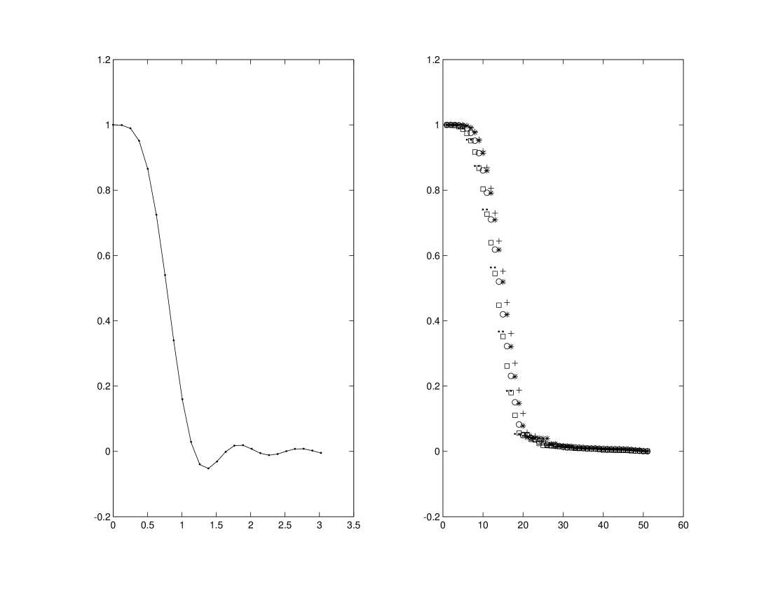
Figure 1: Left. Transfer function of the symmetric Henderson filter, $h=6$, $\nu\in[0,\pi]$ (line) and eigenvalues of the associated circulant matrix $\mathbf{W}$ (dots), $n=51$. Right. Eigenvalue distributions of $\mathbf{W}$ (dots) with asymmetric Musgrave-LC (squares), QL (circles), CQ (stars), LPR filters (pluses) filters, absolute values.

To illustrate, we consider the symmetric 13-term Henderson filter introduced in section 2 and, as an approximation at the boundaries, the LPR estimators and the following asymmetric filters based on a minimum mean square revision error strategy, subject to polynomial constraints:

Linear trend - Constant fit (LC): the asymmetric LC filters arise as the best approximations to the two-sided Henderson filter assuming that $y_{t}$ is linear and imposing the constraint that the weights sum to 1. Hence $\mathbf{U}=\mathbf{i}$, the unit vector. This class contains the well-known Musgrave (1964) surrogate filters that are commonly used to approximate the Henderson filters.

Quadratic trend - Linear fit (QL): the asymmetric QL filters arise as the best approximations to the two-sided Henderson filter assuming that $y_{t}$ is quadratic and imposing the constraint that the estimates are capable of reproducing a first degree polynomial. Hence $\mathbf{U}$ is made of the first two columns of $\mathbf{X}$ whereas $\mathbf{Z}$ contains the third column of $\mathbf{X}$.

Cubic trend - Quadratic fit (CQ): the asymmetric CQ filters arise as the best approximations to the two-sided Henderson filter assuming that $y_{t}$ is a cubic function of time and imposing the constraint that the estimates are capable of reproducing a second degree polynomial. Hence $\mathbf{U}$ is made of the first three columns of $\mathbf{X}$ whereas $\mathbf{Z}$ contains the fourth column of $\mathbf{X}$.

Except for the LPR filters, all of the asymmetric filters are derived here for fixed values of the parameters they depend upon, i.e. $\delta_{r}^{2}/\sigma^{2}$, $r=1,2,3$ for LC, QL and CQ respectively, and are posed equal to the value that gives the Musgrave filter approximating the 13-term Henderson filter, i.e. $\delta_{1}^{2}/\sigma^{2}=4/(3.5^{2}\pi)$. The parameters $\delta_{1},\delta_{2},\delta_{3}$ represent the slope, curvature, and relative inflexion of the trend.

The results are the following: the size of the perturbation is minimum for the Musgrave-LC filters, being $\delta_{W}=0.5835$, and maximum for the LPR filters, for which $\delta_{W}=1.0047$. In the middle, the asymmetric QL, $\delta_{W}=0.8641$ and CQ, $\delta_{W}=0.9876$. As a consequence, the eigenvalue distributions turn out to be slight translations (towards the right) of the absolute transfer function (the gain) of the symmetric filter: this implies an increase in the overall variance of the estimated trend, the increase being greater as long as $\delta_{W}$ increases, as the right panel of figure 1 shows.

The size of the perturbation does not depend on $n$, in that the $n-2h$ central rows of the matrix $\mathbf{S}-\mathbf{W}$ are all null. On the other hand, it is highly influenced by the real time filter (last row of $\mathbf{S}$), applied to estimate the trend at time $t$ using the available observations up to and including $t$. The fact is that, in general, there is a discontinuity in the behaviour of the real time filter with respect to the preceding asymmetric ones, due to the rapid increase of the leverage of the filter, i.e. the weight attached to the observation taken at the same time we are estimating the trend, as long as the span of the filter decreases. The leverage further tends to increase (up to unity) with high degrees of the fitting polynomial (for a formal proof, see Proietti and Luati, 2007). Here, we verify this phenomenon by choosing as smoothing matrix the circulant matrix with first and last rows replaced by any real time filter of the class introduced above. The resulting values of $\delta_{W}$ are almost identical to those obtained when the smoothing matrices with the whole asymmetric filters were considered: for Musgrave-LC it is $\delta_{W}=0.5247$, for QL it is $\delta_{W}=0.8024$, for CQ it is $\delta_{W}=0.9393$, for the LPR filters it is $\delta_{W}=0.9547$. Conversely, all the values of $\delta_{W}$ result greater than $0.95$ provided that the first and last row of $\mathbf{S}$ are replaced by the real time LPR filters, whose leverage is close to one.

Another factor that highly affects the size of the perturbation (and the overall variance of the trend estimates) is the algebraic multiplicity of the eigenvalue $\lambda=1$, that we now show to depend on the degree of the polynomial that the filter is capable of reproducing. The $p-$th degree polynomial reproduction constraints met in section 2 can be written as

$$\langle\mathbf{w}_{t},\mathbf{i}\rangle=1,\;\;\;\;\;\;\langle\mathbf{w}_{t},\mathbf{d}_{q}^{r}\rangle=0\;\;\;\;\;\;\forall t=1,2,...,n$$ (10)

where $\mathbf{w}_{t}^{\prime}$ is the $t$-th row of $\mathbf{S}$, $\mathbf{i}$ is an $n$-dimensional vector of ones and $\mathbf{d}_{q}^{r}=[(-q)^{r},(-q+1)^{r},...,(n-q-1)^{r}]^{\prime},$ with $q=t-1,\mbox{ for }t=1,...,n,r=1,...,p$. As an example, consider a polynomial trend $\mu_{t}=a_{0}+a_{1}+a_{2}^{2}+...+a_{p}^{p}$ and a symmetric filter $\{\mbox{w}_{-h},...,\mbox{w}_{0},...,\mbox{w}_{h}\}$. Then $\hat{\mu}_{t}=\sum_{d=-h}^{h}\mbox{w}_{d}[a_{0}+a_{1}(t+d)+a_{2}(t+d)^{2}+...+a_{p}(t+d)^{p}]=\mu_{t}$ if $\sum_{d=-h}^{h}\mbox{w}_{d}=1$ and $\sum_{d=-h}^{h}d^{r}\mbox{w}_{d}=0$ for $r=1,2,\ldots,p.$ The conditions (10) imply that

$$\mathbf{S}\mathbf{i}=\mathbf{i},\;\;\;\;\;\;\mathbf{S}\mathbf{x}_{r}=\mathbf{x}_{r}$$

where $\mathbf{x}_{r}$ is the vector whose $t$-th coordinate is $a_{0}+a_{1}+a_{2}t^{2}+...+a_{p}t^{r}$, that means that $\mathbf{i}$ and $\mathbf{x}_{r},r=1,2,...,p$, are eigenvectors of $\mathbf{S}$ corresponding to the eigenvalue $\lambda=1$ of algebraic multiplicity equal to $p+1$. It is therefore evident that the greater the algebraic multiplicity of the eigenvalue equal to one, the greater the displacement between the gain function of the filter (equal to one for $\nu=0$ only) and the absolute eigenvalue distribution.

4.3 Reflecting boundary conditions

Besides the class of circulant matrices, another class of matrices with known spectral properties even in finite dimension is the $\tau_{\psi\varphi}$ algebra (Bozzo and Di Fiore, 1995), that is associated with different versions of the Sine and Cosine trasnforms and constitutes a generalisation of the $\tau$ family (Bini and Capovani, 1983). An $n\times n$ matrix $\mathbf{H}$ belongs to the $\tau_{\psi\varphi}$ class if and only if

$$\mathbf{T}_{\psi\varphi}\mathbf{H}=\mathbf{H}\mathbf{T}_{\psi\varphi}$$

where

$$\mathbf{T}_{\psi\varphi}=\left[\begin{array}[]{rrrrr}\psi&1&0&\cdots&0\\ 1&0&1&\ddots&0\\ 0&1&\ddots&\ddots&0\\ \vdots&\ddots&\ddots&0&1\\ 0&\ldots&0&1&\varphi\\ \end{array}\right]$$

and $\psi,\varphi=0,1,-1.$ The elements $\mbox{h}_{ij}$ of the matrices in $\tau_{\psi\varphi}$ satisfy the cross sum property $\mbox{h}_{i-1j}+\mbox{h}_{i+1j}=\mbox{h}_{ij-1}+\mbox{h}_{ij+1}$ subject to boundary conditions determined by $\psi$ and $\varphi$. For the original $\tau$ algebra arising when $\psi=\varphi=0$ the boundary conditions are $\mbox{h}_{0j}=\mbox{h}_{i0}=\mbox{h}_{n+1j}=\mbox{h}_{in+1}=0$, $i,j=1,...,n$ and all the matrices in $\tau$ can be then derived given their first row elements. Still based on the first row of $\mathbf{H}$ but more appropriate for our purposes, since it allows to obtain the eigenvalues and eigenvectors of $\mathbf{H}$ in $\tau_{\psi\varphi}$ in an amenable form, is the following way to construct $\mathbf{H}$ as a linear combination of powers of $\mathbf{T}_{\psi\varphi}$ (see Bini and Capovani, 1983, Proposition 2.2). Let $\mathbf{h}^{\prime}=[\mbox{h}_{1},\mbox{h}_{2},...,\mbox{h}_{n}]$ be the first row of $\mathbf{H}$. Then

$$\mathbf{H}=\sum_{j=1}^{n}c_{j}\mathbf{T}_{\psi\varphi}^{j-1}$$

where $\mathbf{c}$ is the solution of the upper triangular system $\mathbf{Q}\mathbf{c}=\mathbf{h}$ and $\mathbf{Q}$ is the matrix whose $j$-th column equals the first column of $\mathbf{T}_{\psi\varphi}^{j-1}$. It follows that the eigenvalues of $\mathbf{H}$ are given by

$$\xi_{i}=\sum_{j=1}^{n}\vartheta_{i}^{j-1}c_{j}$$ (11)

where $\vartheta_{i},i=1,..,n,$ are the eigenvalues of $\mathbf{T}_{\psi\varphi}.$ The eigenvectors of $\mathbf{H}$ are the same of $\mathbf{T}_{\psi\varphi}$.

Let us consider the reflecting hypothesis such that the first missing observation is replaced by the last available observation, the second missing observation is replaced by the previous to the last observation and so on, that for a two-sided $2h+1$-term estimator corresponds to the real time filter $\{\mbox{w}_{h},\mbox{w}_{h-1}+\mbox{w}_{h},...,\mbox{w}_{1}+\mbox{w}_{2},\mbox{w}_{0}+\mbox{w}_{1}\}$, made of $h+1$ terms. With the constraint of being centrosymmetric, the reflecting matrix $\mathbf{H}$ belongs to the $\tau_{11}$ algebra and its first row is the vector

$$\mathbf{h}^{\prime}=\left[\mbox{w}_{0}+\mbox{w}_{1},\mbox{w}_{1}+\mbox{w}_{2},\mbox{w}_{2}+\mbox{w}_{3},...,\mbox{w}_{h-1}+\mbox{w}_{h},\mbox{w}_{h},0,...,0\right].$$ (12)

With these premises, we are able to construct $\mathbf{H}\in\tau_{11}$ corresponding to the symmetric filter $\{\mbox{w}_{-h},...,\mbox{w}_{0},\mbox{w}_{1},...,\mbox{w}_{h}\}$ and to derive the following result where, for sake of notation, we use the Pochhammer symbol $(j)_{q}=j(j+1)(j+2)...(j+q-1)$, for $q=0,1,...,\left\lfloor\frac{h-j-1}{2}\right\rfloor$, the latter term denoting the largest integer less than or equal to $\frac{h-j-1}{2}$.

Theorem 2 Let $\mathbf{S}$ be an $n\times n$ smoothing matrix associated with the symmetric filter $\{\mbox{w}_{-h}$, $...$, $\mbox{w}_{0},...,\mbox{w}_{h}\}$, and let $\mathbf{H}$ be the corresponding matrix in $\tau_{11}$. Hence, $\forall\lambda\in\sigma(\mathbf{S})$, $\exists i\in\{1,2,..,n\}$ such that

$$\left|\lambda-\xi_{i}\right|\leq\delta_{H}$$

where

$$\xi_{i}=\sum_{j=1}^{h+1}\left(2\cos\frac{(i-1)\pi}{n}\right)^{j-1}\left[\mbox{w}_{j-1}+\sum_{q=0}^{\left\lfloor\frac{h-j-1}{2}\right\rfloor}\frac{(-1)^{q+1}(j)_{q}}{(q+1)!}(j+2q+1)\mbox{w}_{j+2q+1}\right]$$ (13)

and $\delta_{H}=\|\mathbf{S}-\mathbf{H}\|_{2}$.

The proof is in section 7. As by-product, theorem 2 gives the eigenvalues of $\mathbf{H}\in\tau_{11}$, with first row equal to (12), as an explicit function of the filter weights, as shown in (13). The corresponding eigenvectors are known (Bozzo and Di Fiore, 1995) and given by

$$\mathbf{z}_{i}=k_{i}\left[\cos\frac{(2j-1)(i-1)\pi}{2n}\right]_{j},j=1,2,...,n$$ (14)

with $k_{i}=\frac{1}{\sqrt{2}}$ for $i=1$ and $k_{i}=1$ for $i>1.$ The inferential procedures that will be introduced in the following section are based on the eigenvalues and eigenvectors given by (13) and (14), respectively. In the sequel, we discuss the merit of assuming reflecting rather than circulant boundary conditions, i.e. of basing the inference on theorem 2 rather then on theorem 1.

Indeed, there are several advantages in adopting the approximation for $\mathbf{S}$ given by $\mathbf{H}\in\tau_{11}$ instead of the circulant approximation provided by $\mathbf{W}$. First, all the operators belonging to $\tau$ algebras have real eigenvalues and eigenvectors. All the computations related to this class can therefore be done in real arithmetic. Secondly, the reflecting hypothesis undertaken by the $\tau_{11}$ algebra is more appropriate than that of a circular process when the signal is a non stationary function of time, as is the case when we are interested in its estimate. It should be reminded that the estimation methods considered so far are local, so that the boundary conditions only concern a neighborhood of the ending observations. For fixed bandwidth methods this means that only $h,h+1,...,2h$ observations are involved in the asymmetric filtering; if a nearest neighbourhood approach is followed, then $2h+1$ observations will be weighted even at the extremes of the series. Another aspect that deserves to be remarked on concerns the absolute size of the perturbation (an overestimate of the true distance about eigenvalues), which is smaller for reflecting than for circulant boundary conditions, i.e. $\delta_{H}<\delta_{W}$. In fact, in general, Circulant-to-Toeplitz corrections produce perturbations that are not smaller than Tau-to-Toeplitz corrections, since while $\mathbf{H}$ is structured as (9), the circulant $\mathbf{W}$ has nonzero corrections in the top right and bottom left $h\times h$ blocks. When the matrix elements are the same, this results in a greater perturbation. Table 1 illustrates this property for the class of approximate filters considered before.

Table 1: Values of $\delta$ for $h=6$, $\tau_{11}$ and circulant algebras, approximate asymmetric filters.

	LC	QL	CQ	LPR
$\delta_{H}$ (Reflecting)	0.1608	0.3817	0.7493	0.8351
$\delta_{W}$ (Circulant)	0.5835	0.8641	0.9876	1.0047

Finally, as we anticipated in the preceding subsection, the main aspect concerning the $\tau_{11}$ approximation is that $\mathbf{H}$ has $n$ distinct eigenvalues compared to the at most $\frac{n-1}{2}+1$ of $\mathbf{W}$, compare the left panel of figure 2 with left panel of figure 1. What follows is that the eigenvalue distribution of any smoothing matrix $\mathbf{S}$ having the form of (9) can be approximated by that of the corresponding $\mathbf{H}\in\tau_{11}$, having the same submatrix-structure, with a deviation smaller than $\delta_{H}$. The same order deviation occurs between the eigenvalue distribution of $\mathbf{S}$ and the transfer function of the corresponding symmetric filter, as showed in the right panel of figure 2.

To conclude our discussion on the eigenvalues of $\mathbf{S}$, we remark that their complex part is merely generated by the finite approximation and not related to the phase that in general affects the asymmetric filters. This can be easily understood by means of a counterexample: the matrix associated with a cubic smoothing spline (see Whaba, 1990, and Green and Silverman, 1994) is symmetric, so that its eigenvalues are real even if the asymmetric filters do produce phase shifts.

We now consider the eigenvectors. In the preceding section we have proven that if the filter reproduces a polynomial of order $p$, then there exist $p+1$ eigenvectors, associated with the eigenvalue $\lambda=1$, that describe a constant ($r=0$), linear ($r=1$), quadratic ($r=2$), cubic ($r=3$) and so on up to a $p$-th order polynomial function of the time.

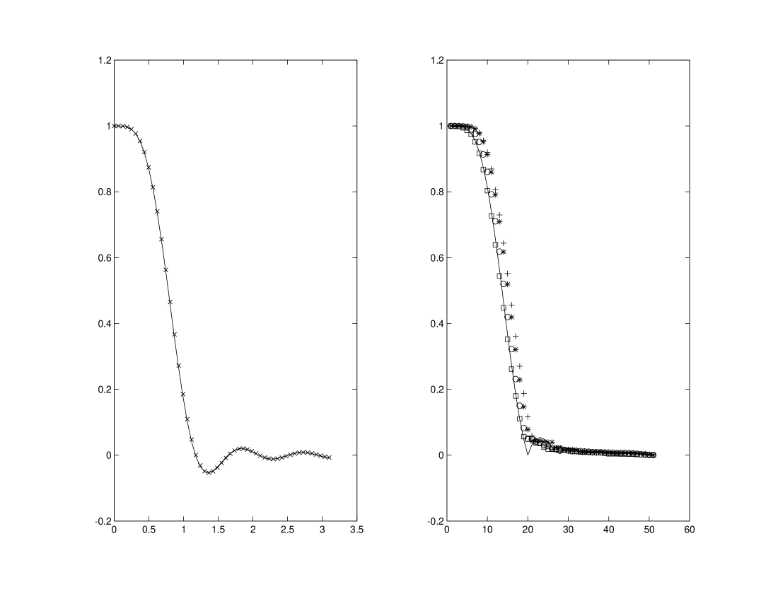
Figure 2: Left. Transfer function of the symmetric Henderson filter, $h=6$, $\nu\in[0,\pi]$ (line) and eigenvalues of the associated reflecting matrix $\mathbf{H}$ (crosses), $n=51$. Right. Gain function of the symmetric Henderson filter, $h=6$ (line) and eigenvalue distributions of $\mathbf{S}$ with asymmetric Musgrave-LC (squares), QL (circles), CQ (stars), LPR filters (pluses) filters.

In general, the analytical expression of the eigenvectors of a smoothing matrix cannot be derived using the perturbation theory, not even in an approximate form. However, evaluating the action of $\mathbf{S}$ on the eigenvectors of $\mathbf{H}$, we are able to show that, unless for the boundaries, the latent components of $\mathbf{S}$ can be fairly approximated by those of $\mathbf{H}$. In fact, let us decompose the time series $\mathbf{y}$ as a linear combination of the $n$ known real and orthogonal latent components represented by the eigenvectors of $\mathbf{H}$,

$$\mathbf{y}=\theta_{1}\mathbf{z}_{1}+\theta_{2}\mathbf{z}_{2}+...+\theta_{n}\mathbf{z}_{n}$$

where the $\mathbf{z}_{i}$ are given by (14) and $\mbox{\boldmath$\theta$}=[\theta_{1},...,\theta_{n}]^{\prime}$ is a vector of coefficients. It follows from theorem 2 that

$$\mathbf{S}\mathbf{y}=\sum_{i=1}^{n}\theta_{i}\xi_{i}\mathbf{z}_{i}+\sum_{i=1}^{n}\theta_{i}\mbox{\boldmath$\Delta$}_{\mathbf{H}}\mathbf{z}_{i}$$

where $\mbox{\boldmath$\Delta$}_{\mathbf{H}}\mathbf{z}_{i}$ is a vector of zeros except for the first and last $h$ coordinates, i.e.

$$\mbox{\boldmath$\Delta$}_{\mathbf{H}}\mathbf{z}_{i}=\left[\begin{array}[]{ccc}\mathbf{z}_{i}^{*}\\ \mathbf{0}\\ \mathbf{E}_{h}\mathbf{z}_{i}^{*}\end{array}\right]$$

and $\mathbf{z}_{i}^{*}=\sum_{j=1}^{q}(\mathbf{S}_{ij}-\mathbf{H}_{ij})\mbox{z}_{ij}$ for $q=h+1,...,2h$ and $i=1,2,...,h$. Due to the fact that the elements of both $\mathbf{S}$ and $\mathbf{H}$ add up to one and their absolute values are in general smaller than one, the values in $\mathbf{z}_{i}^{*}$ and in $\mathbf{E}_{h}\mathbf{z}_{i}^{*}$ are almost zero. This holds not only for $n\gg h$, which is the case when we usually apply local filters, but also for $n$ close to $h$, as figure 3 illustrates in the limiting case of $n=2h+1$, where the approximation concerns the maximum number of boundary approximations, namely $n-1$.

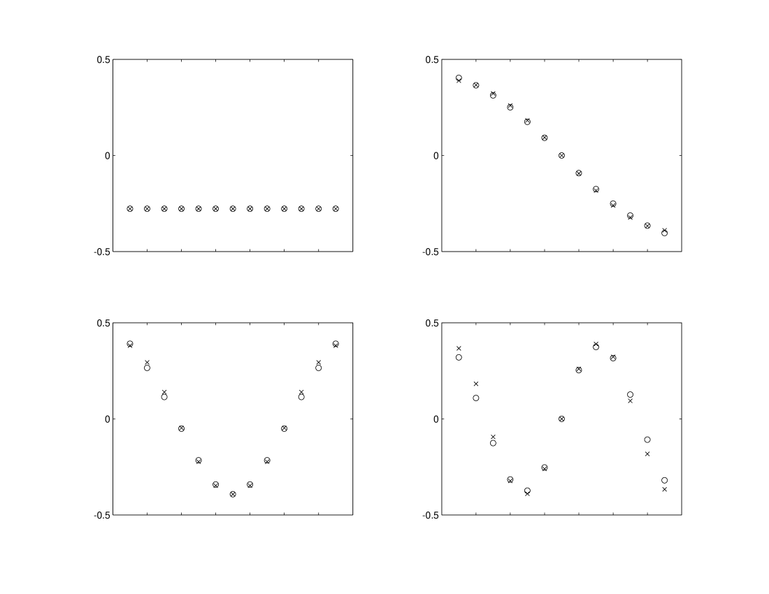
Figure 3: Coordinates of the first four eigenvectors $\mathbf{z}_{i}$, $i=1,2,3,4$ of $\mathbf{H}$ (crosses) and of $(\mathbf{I}+\mbox{\boldmath$\Delta$}_{\mathbf{H}})\mathbf{z}_{i}$ (circles) plotted against $t=1,2,...n$, $n=13,h=6$, symmetric Henderson filter.

5 Filter design in the time domain

The results of the preceding sections are applied for a filter design in time domain. The aim is to obtain estimates with smaller variance and almost equal bias than those produced by $\mathbf{S}$. The method consists of modifying $\mathbf{S}$ so that $n-k$ high frequency noisy components that the filter is not capable of eliminating are given zero weight. This is done through the spectral decomposition of $\mathbf{H}$. The choice of $k$ i.e. of the cut-off eigenvalue $\xi_{k}$ will be discussed later in this section.

Decomposing $\mathbf{S}=\mathbf{H}+\mbox{\boldmath$\Delta$}_{\mathbf{H}}$ and $\mathbf{H}=\mathbf{Z}\mathbf{\mathcal{X}}\mathbf{Z}^{\prime}$, where $\mathbf{\mathcal{X}}=\mbox{diag}\{\xi_{1},\xi_{2},...,\xi_{n}\}$, and writing $\mathbf{y}=\mathbf{Z}\mbox{\boldmath$\theta$}$, we get

$$\begin{array}[]{lll}\mathbf{S}\mathbf{y}&=&\mathbf{Z}\mathbf{\mathcal{X}}\mbox{\boldmath$\theta$}+\mbox{\boldmath$\Delta$}_{\mathbf{H}}\mathbf{Z}\mbox{\boldmath$\theta$}\\ &\approx&\mathbf{Z}\mathbf{\mathcal{X}}_{k}\mbox{\boldmath$\theta$}+\mbox{\boldmath$\Delta$}_{\mathbf{H}}\mathbf{Z}\mbox{\boldmath$\theta$}\end{array}$$

where $\mathbf{\mathcal{X}}_{k}$ is the matrix obtained by replacing with zeros the eigenvalues of $\mathbf{H}$ that are smaller than a cut-off eigenvalue $\xi_{k}$ and $\mbox{\boldmath$\Delta$}_{\mathbf{H}}\mathbf{Z}\mbox{\boldmath$\theta$}$ is a null vector except for the first and last elements that account for the boundary conditions. Turning to the original coordinate system and arranging the boundaries, we get the new estimator

$$\begin{array}[]{lll}\mathbf{S}_{k}&=&\mathbf{H}_{k}+\mbox{\boldmath$\Delta$}_{k}+\mbox{\boldmath$\Delta$}_{\mathbf{H}}\\ &=&\mathbf{H}_{(k)}+\mbox{\boldmath$\Delta$}_{\mathbf{H}}\end{array}$$

where $\mathbf{H}_{(k)}$ is the matrix with boundaries equal to those of $\mathbf{H}$ and interior equal to that of $\mathbf{H}_{k}=\mathbf{Z}\mathbf{\mathcal{X}}_{k}\mathbf{Z}^{\prime}$. In other words, $\mathbf{H}_{(k)}$ is structured like (9) with $\mathbf{H}_{k}^{a}=\mathbf{H}^{a}$, $\mathbf{H}_{k}^{a*}=\mbox{t}(\mathbf{H}^{a})$ and $\mathbf{H}_{k}^{s}=[\mathbf{Z}\mathbf{\mathcal{X}}_{k}\mathbf{Z}^{\prime}]^{s}$. Hence a new smoothing matrix is obtained, $\mathbf{S}_{k}$, and consequently new trend estimates, say $\hat{\mathbf{m}}_{k}$.

In practice, the procedure is much easier to apply. In fact, given a symmetric filter, it consists of: obtaining $\mathbf{H}$, replacing it by $\mathbf{H}_{k}$ and then adjusting the boundaries with suitable chosen asymmetric filters to get $\mathbf{S}_{k}$. Besides simplicity and variance improvement in the interior, this procedure allows a full choice of the set of asymmetric weights. Indeed, in the examples we shall illustrate at the end of this section, due to the strong impact of the real time filter respect to all the asymmetric ones, we will replace only the last row of $\mathbf{H}_{k}$.

5.1 Bias-variance trade off

Let us assume that $\mbox{\boldmath$\epsilon$}\sim\mathcal{N}(0,\sigma^{2}\mathbf{I})$. The variance of the estimates obtained by $\mathbf{S}$ is given by $V(\hat{\mathbf{m}})=V(\mathbf{S}\mathbf{y})=\mathbf{S}\sigma^{2}\mathbf{I}\mathbf{S}^{\prime}$. It follows that

$$V(\hat{\mathbf{m}})-V(\hat{\mathbf{m}}_{k})=\sigma^{2}[\mathbf{Z}(\mathbf{\mathcal{X}}^{2}-\mathbf{\mathcal{X}}_{k}^{2})\mathbf{Z}^{\prime}+(\mathbf{H}-\mathbf{H}_{k})\mbox{\boldmath$\Delta$}_{\mathbf{H}}^{\prime}+\mbox{\boldmath$\Delta$}_{\mathbf{H}}(\mathbf{H}-\mathbf{H}_{k})^{\prime}-(\mathbf{H}_{k}\mbox{\boldmath$\Delta$}_{k}^{\prime}+\mbox{\boldmath$\Delta$}_{k}\mathbf{H}_{k}^{\prime})]$$

where $\mathbf{Z}(\mathbf{\mathcal{X}}^{2}-\mathbf{\mathcal{X}}_{k}^{2})\mathbf{Z}^{\prime}$ is the main contribution to the variance in the interior and is greater than zero in the sense of a positive definite matrix; the two summands left restitute a matrix with non null first and last $2h$ rows only, given that $\mbox{\boldmath$\Delta$}_{\mathbf{H}}$ and $\mbox{\boldmath$\Delta$}_{k}$ have top left and bottom right nonzero blocks of dimension $h\times 2h$. So, even if they mainly account for the variance at the boundaries, they also contribute to the variance in the interior. However, for $h\ll n$ the contribution is negligible with respect to that of the first summand and it is common to both $\hat{\mathbf{m}}$ and $\hat{\mathbf{m}}_{k}$.

The bias is given by $B(\hat{\mathbf{m}})=\mbox{\boldmath$\mu$}-E(\hat{\mathbf{m}})=\mbox{\boldmath$\mu$}-(\mathbf{H}+\mbox{\boldmath$\Delta$}_{\mathbf{H}})\mbox{\boldmath$\mu$}=[\mathbf{I}-(\mathbf{H}+\mbox{\boldmath$\Delta$}_{\mathbf{H}})]\mbox{\boldmath$\mu$}.$ As introduced by the filtering procedure, the bias is smaller as long as $\mathbf{S}$ tends to the identity matrix (in terms of the eigenvalues of $\mathbf{S}=\mathbf{I}$, there are $n$ eigenvalues equal to one and therefore the filter is capable of reproducing an $n$-degree polynomial interpolating the data, i.e. the series itself). Comparing the bias of the two estimators we see that

$$B(\hat{\mathbf{m}})-B(\hat{\mathbf{m}}_{k})=\left[\mathbf{Z}(\mathbf{\mathcal{X}}_{k}-\mathbf{\mathcal{X}})\mathbf{Z}^{\prime}+\mbox{\boldmath$\Delta$}_{k}\right]\mbox{\boldmath$\mu$}$$

and so a measure of the discrepancy between the bias of $\hat{\mathbf{m}}_{k}$ and that of $\hat{\mathbf{m}}$, in the interior, is

$$\frac{1}{n}\mbox{ tr }\{\mathbf{\mathcal{X}}_{k}-\mathbf{\mathcal{X}}\}=-\frac{1}{n}\sum_{i=n-k+1}^{n}\xi_{i}.$$

In general $\mbox{ tr }\{\mathbf{\mathcal{X}}_{k}-\mathbf{\mathcal{X}}\}$ is a negative quantity that normalised by $n$ is negligible, given that the last $n-k$ eigenvalues ar almost zero, as follows by (13).

The choice of $k$ is a further balancing of the trade-off between bias and variance of the filter. The trend in the interior is made smoother without sensibly increasing the bias. There are several options regarding how to choose $k$. One of them, which we shall adopt in our illustrations, consists of selecting $k$ or equivalently $\xi_{k}$ that minimises the distance of the eigenvalue distribution of $\mathbf{H}$ with that of the ideal low pass filter having first $k$ eigenvalues equal to one and and last $n-k$ equal to zero. In other words, we look for $k$ such that

$$f(k)=\|\mathbf{i}_{(k)}-\mbox{\boldmath$\xi$}\|^{2}$$ (15)

is minimum, where $\mathbf{i}_{(k)}$ is an $n$ dimensional vector with first $k$ coordinates equal to one and the remaining equal to zero, whereas $\mbox{\boldmath$\xi$}=[\xi_{1},\xi_{2},...,\xi_{n}]^{\prime}$ and the $\xi_{i}$ are given by (13). The function $f(k)=\sum_{i=1}^{k}(1-\xi)^{2}-\xi_{i}^{2}$ can be written as $f(k)=f(k-1)+(1-\xi_{k})^{2}-\xi_{k}^{2}=f(k-1)+(1-2\xi_{k})$ and therefore reaches its minimum for $\xi_{k}=0.5.$ This strategy is equivalent to finding the cut-off frequency that minimises the distance between the transfer functions of the symmetric filter and of the ideal low-pass filter

$$\int_{-\pi}^{\pi}|I(\nu)-H(\nu)|^{2}d\nu$$

where $I(\nu)=1$ for $\nu<\frac{2\pi}{p}$and $I(\nu)=0$ otherwise. The equivalence is based on the relation between time and frequency domain. In fact, for a fixed a cut-off frequency $\nu=\nu_{k}$, the cut-off time $k=\frac{\nu_{k}n}{\pi}$ is obtained with a precision that increases as long as $n$ is large. For instance, if we are given monthly data and are interested in removing 10-month cycles that can be wrongly interpreted as turning points of the trend curve, then we may replace by zeros all the eigenvalues smaller than $\xi_{k}$ with $k=\frac{2n}{10}.$

Finally, we would like to remark that whenever the interest is in the smoothness of the new estimator rather than in the exact value of $k$, a graphical inspection method may be appropriate. Having plotted the eigenvalue distribution, a suitable cut-off eigenvalue may be directly viewed. If the choice of $k$ is not related to formal inferential procedure (e.g. restrictions on the bias) this method works well.

5.2 Empirical analysis

In this section we provide illustrations of the eigenvalue-based method for reducing the variance of the trend estimates obtained with a given symmetric filter that is applied to real data. As a symmetric estimator, we consider the $13$ term Henderson (1916) filter, which plays a prominent role in empirical applications, especially for trend estimation within the X-11 filter, which is an integral part of the X-12-ARIMA procedure, the official seasonal adjustment procedure in the U.S., Canada, the U.K. and many other countries. See Dagum (1980), Findley et al. (1998) and Ladiray and Quenneville (2001) for more details. As for the asymmetric filters, the reflecting have been chosen except for the case of the real time filter. In particular, the QL (Proietti and Luati, 2007) and Musgrave (1964) real time filters discussed in section 4.2 have been applied and compared. The smoothing matrix $\mathbf{S}$ is therefore equal to $\mathbf{H}$ except for the last row changed. To obtain $\mathbf{S}_{k}$ we find the spectral decomposition of $\mathbf{H}$ and select the cut-off eigenvalue according to (15), i.e. $\xi_{k}=0.5$.

Our first illustration deals with the Italian index of industrial production. The top panel of figure 4 represents the original series with the trend estimates $\hat{\mathbf{m}}$ (dotted line) and $\hat{\mathbf{m}}_{k}$ (continuous line). The gain in smoothness obtained using the latter estimator is not so evident in the whole series but can be clearly seen in the central panel of figure 4, where a subset of the data is represented. The estimates obtained by $\hat{\mathbf{m}}_{k}$ are less sensitive to the fluctuations of the series, note in particular the behaviour in the period ranging from June 1999 to June 2001 when the series is slightly increasing: the original filter estimates are sensible to noisy fluctuations that do not affect the modified version where highly noisy components are removed instead of just smoothed. The bottom panel shows the last year estimates to give an idea of a comparison among asymmetric filters: the Musgrave real time filter (dots) behaves almost like the reflecting one (dotted line) whereas the QL real time filter (continuous line) follows the series increase.

Analog considerations apply to our second illustration, which concerns the series of retails of Euro area 4, see figure 5. This series is affected by an increase in variability even during periods of stationarity of the trend, as the top panel of the figure shows. The 13-term Henderson filter (dotted line) is known to be particularly reacting to short cycles that, if not smoothed enough, can be falsely interpreted as false turning points. The central part of figure 5 illustrates that the modified estimator (continuous line) where eigenvalues smaller than 0.5 are replaced by zeros produces smoother trend values without affecting the capability of catching true turning points, such as that occurred in November 1994. As in the previous case, in the bottom panel of figure 5 the last year estimates obtained with Musgrave (dots), the reflecting (dotted line) and the QL (continuous line) real time filters are illustrated. Even in this case, the QL reacts to the changes in the direction of the series more than the other two estimators which behave almost in the same manner.

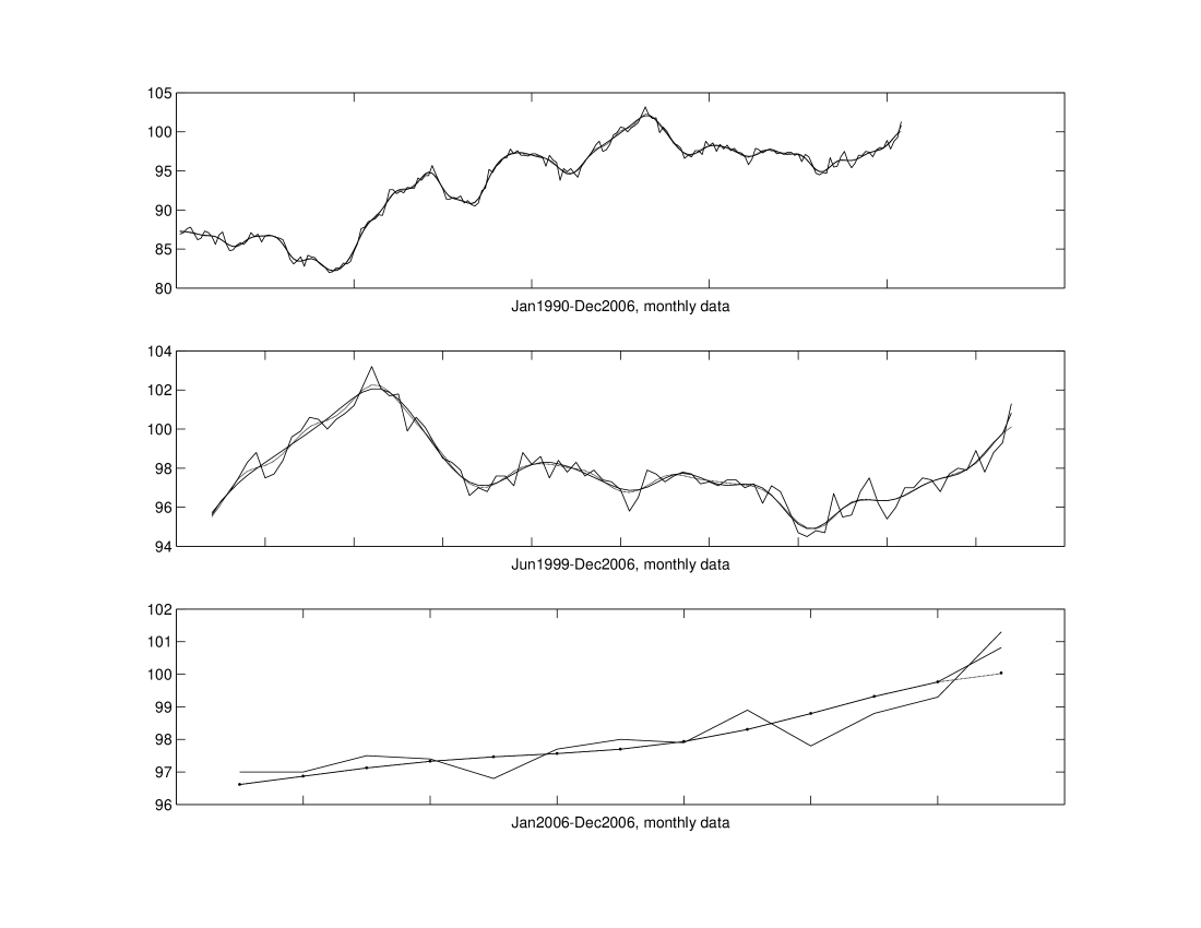
Figure 4: Index of Industrial Production, Italy. Source: Istat. Top and center. Original series with estimates obtained by $\mathbf{H}$ (dotted line) and by $\mathbf{H}^{*}$(continuous line). Bottom. Real time estimates by QL (continuous line), reflecting (dotted line) and Musgrave (dots) real time filters.

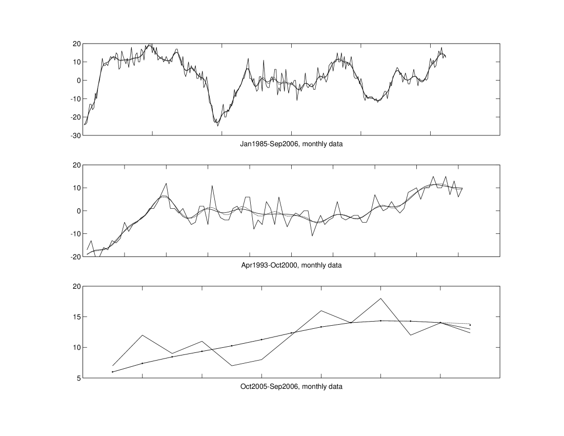
Figure 5: Euro Area Industry, Retail Ea4. Source: European commission. Top and center. Original series with estimates obtained by $\mathbf{H}$ (dotted line) and by $\mathbf{H}^{*}$(continuous line). Bottom. Real time estimates by QL (continuous line), reflecting (dotted line) and Musgrave (dots) real time filters.

6 Concluding remarks

This paper provided a decomposition of time series in periodic latent components that depends on the underlying trend estimation method. In particular, given a symmetric local polynomial regression estimator with reflecting boundary conditions, the latent components are given exactly by equation (14). These will be smoothed by an amount equal to (13). If different asymmetric filters for current trend estimation are adapted at the boundaries, then an approximation whose size was given in theorem 2 occurs in the eigenvalue distribution.

Concerning the latter, it was shown in the paper that, in finite dimension, an approximated version of the fundamental eigenvalue distribution theorem holds. In fact, the eigenvalue distribution of a trend filter matrix turned out to be a discrete approximation of the the transfer function of the corresponding symmetric filter. Once again, the size of the approximation depends on boundary conditions. Circular and reflecting boundary conditions were illustrated and discussed. In any case, it emerged that as long as the locally weighted regression method is capable of reproducing a high degree polynomial trend, the approximation to the transfer function of the filter becomes worse, essentially due to the exploding behavior of the real time filter when the degree of the fitting polynomial increases.

It followed that, as well as the transfer function, the eigenvalue distribution represents a measure of the overall variance left in the input series by the smoothing procedure. More relevant, the decomposition in periodic latent component to which smoothing eigenvalues are associated constituted a framework for reducing the variance of the estimates.

In fact, based on the analytical knowledge of the eigenvectors and eigenvalues, it was possible to improve the inferential properties of a given filter by annihilating noisy components that would have been otherwise only smoothed. The selection of a cut-off eigenvalue after which all the components received zero weight was discussed and new filters with smaller variance and almost equal bias to the original one were so derived. Applications to real data showed the variance improvement, especially for what concerns short cycles that may wrongly be interpreted as turning points of the trend-cycle.

7 Appendix

Proof of theorem 1 The matrix $\mathbf{S}$ can be written as $\mathbf{S}=\mathbf{W}+\mbox{\boldmath$\Delta$}_{\mathbf{W}}$, where $\mbox{\boldmath$\Delta$}_{\mathbf{W}}=\mathbf{S}-\mathbf{W}$. The circulant matrix $\mathbf{W}$ is diagonalised by the Fourier matrix

$$\mbox{\boldmath$\Omega$}=\frac{1}{\sqrt{n}}[\omega^{(i-1)(j-1)}]_{ij},$$

$i,j=1,...,n$, satisfying $\|\mbox{\boldmath$\Omega$}\|_{2}\|\mbox{\boldmath$\Omega$}^{-1}\|_{2}=1$, and its spectrum is $\sigma(\mathbf{W})=\{\zeta_{1},\zeta_{2},...,\zeta_{n}\}$, with

$$\zeta_{i}=\sum_{d=0}^{h}\mbox{w}_{d}\omega^{(i-1)d}+\sum_{d=-h}^{-1}\mbox{w}_{d}\omega^{(i-1)(n+d)}.$$

Setting $\delta_{W}=\|\mbox{\boldmath$\Delta$}_{\mathbf{W}}\|_{2}$, the thesis follows from the Bauer-Fike perturbation theorem applied choosing the $2$-norm as an absolute norm (Bauer and Fike, 1960). $\blacksquare$

Proof of theorem 2 Let us write $\mathbf{S}=\mathbf{H}+\mbox{\boldmath$\Delta$}_{\mathbf{H}}$. The first part of the proof is analog to the proof of theorem 1, provided that the matrix $\mathbf{H}$ is diagonalised by the orthogonal matrix

$$\mathbf{Z}=\sqrt{\frac{2}{n}}\left[k_{j}\cos\frac{(2i-1)(j-1)\pi}{2n}\right]_{ij},i,j=1,2,...,n$$

where $k_{j}=\frac{1}{\sqrt{2}}$ for $j=1$ and $k_{j}=1$ for $j>1$ which satisfies $\|\mathbf{Z}\|_{2}\|\mathbf{Z}^{-1}\|_{2}=1$. The spectrum of $\mathbf{H}$ is $\sigma(\mathbf{H})=\{\xi_{1},\xi_{2},...,\xi_{n}\}$, where

$$\xi_{i}=\sum_{j=1}^{n}\left(2\cos\frac{(i-1)\pi}{n}\right)^{j-1}c_{j}$$

which follows by (11) and by the fact that the eigenvalues of $\mathbf{T}_{11}$ are (Bini and Capovani, 1983)

$$\vartheta_{i}=2\cos\frac{(i-1)\pi}{n}.$$

Setting $\delta_{H}=\|\mbox{\boldmath$\Delta$}_{\mathbf{H}}\|_{2}$ and applying the Bauer-Fike theorem with the $2$-norm as an absolute norm gives

$$\left|\lambda-\sum_{j=1}^{n}\left(2\cos\frac{(i-1)\pi}{n}\right)^{j-1}c_{j}\right|\leq\delta_{H}.$$

We now prove that $c_{j}=0$ for $j>h+1$, so that the above summation involves just $h+1$ terms instead of $n$. It follows by the Cramer rule that, explicitly,

$$c_{j}=\frac{\det\mathbf{Q}\left[j,\mathbf{h}\right]}{\det\mathbf{Q}}$$

where $\mathbf{Q}\left[j,\mathbf{h}\right]$ is the matrix obtained replacing the $j$-th column of $\mathbf{Q}$ by the vector $\mathbf{h}$. The matrix $\mathbf{Q}$ is upper triangular with ones on the diagonal so its its determinant is equal to one and since the generic element $h_{j}$ of $\mathbf{h}$ is null for $j>h+1$ it follows that $\det\mathbf{Q}\left[j,\mathbf{h}\right]=0$ and $c_{j}$ will be null as well.

Finally, we prove that

$$c_{j}=\mbox{w}_{j-1}+\sum_{q=0}^{\left\lfloor\frac{h-j-1}{2}\right\rfloor}\frac{(-1)^{q+1}(j)_{q}}{(q+1)!}(j+2q+1)\mbox{w}_{j+2q+1}.$$ (16)

This expression can be directly verified by calculating $\det\mathbf{Q}\left[j,\mathbf{h}\right]$ for all $j$. Here in the following, we prove it by induction over $j=1,...,h+1$, with $h\in\mathbb{N}$.

• For $j=1$, $c_{1}=\mbox{w}_{0}+\sum_{q=0}^{\frac{h-2}{2}}(-1)^{q+1}2\mbox{w}_{2q+2}$ which follows by $(1)_{q}=q!$ and by simple algebra. The linear system $\mathbf{Q}\mathbf{c}=\mathbf{h}$ can be written as $\mathbf{c}=\mathbf{Q}^{-1}(\mathbf{h}_{1}+\mathbf{h}_{2})$ with $\mathbf{h}_{1}=[\mbox{w}_{0},\mbox{w}_{1},...,\mbox{w}_{h},0,...,0]^{\prime}$ and $\mathbf{h}_{2}=[\mbox{w}_{1},\mbox{w}_{2},...,\mbox{w}_{h},0,...,0]^{\prime}$, both $n$-dimensional vectors. Since the first row of $\mathbf{Q}^{-1}$ is the vector $[1,-1,-1,1,1,-1,-1,...]$ we have that $c_{1}=(\mbox{w}_{0}+\mbox{w}_{1})-(\mbox{w}_{1}+\mbox{w}_{2})-(\mbox{w}_{2}+\mbox{w}_{3})+(\mbox{w}_{2}+\mbox{w}_{4})+...+(-1)^{\left\lfloor\frac{h-2}{2}\right\rfloor+1}2\mbox{w}_{2\left\lfloor\frac{h-2}{2}\right\rfloor+2}$ and therefore (16) holds for $j=1$.

• For $j=h$, $c_{h}=\mbox{w}_{h-1}$ as it is immediate to see given that the summation in $q$ was defined for non negative values of $\frac{h-j-1}{2}$. All the more so, it implies that $c_{h+1}=\mbox{w}_{h}$. Hence we have showed that (16) holds for $j=1$ and that, if it holds for $j=h$ then it holds for $j=h+1$. This proves that (16) is true for all $h\in\mathbb{N}$. The proof of theorem 2 is therefore complete $\blacksquare$

Acknowledgements The authors would like to kindly thank Dario Bini for the precious suggestions and the useful discussions. This paper has been presented at the 56th Session of the ISI 2007 Lisbon, August 22-29, 2007 and at the Workshop Two Days of Linear Algebra, Bologna, 6-7 March 2008. We are especially grateful to Daniele Bertaccini Enrico Bozzo, Fabio Di Benedetto, Marco Donatelli and Valeria Simoncini for their very competent comments.

References

• Anderson, T.W. (1971), The Statistical Analysis of Time Series, Wiley.

• Bauer F., Fike C. (1960), Norms and Exclusion Theorems, Numerische Mathematik, 2, 137-141.

• Bini D., Capovani M. (1983), Spectral and computational properties of band symmetric Toeplitz matrices, Linear Algebra and its Applications, 52/53, pp. 99-126 .

• Bini D., Favati P. (1993), On a matrix algebra related to the discrete Hartley transform. SIMAX, 14, 2, 500-507

• Bloomfield, P. (2000). Fourier Analysis of Time Series. An Introduction, Second edition, Wiley.

• Böttcher A., Grudsky, S.M. (2005), Spectral Properties of Banded Toeplitz Matrices, Siam.

• Bozzo E., Di Fiore C. (1995) On the use of certain matrix algebras associated with discrete trigonometric transforms in matrix displacement decomposition, Siam J. Matrix anal. Appl., 16, 1, 312-326.

• Buja A., Hastie T.J., Tibshirani R.J.(1989), Linear Smoothers and Additive Models, The Annals of Statistics, 17, 2, 453-555

• Cantoni A., Butler P. (1976), Eigenvalues and eigenvectors of symmetric centrosymmetric matrices, Linear Algebra and its Applications, 13, 275-288.

• Cleveland, W.S. and Loader, C.L. (1996). Smoothing by Local Regression: Principles and Methods. In W. Härdle and M. G. Schimek, editors, Statistical Theory and Computational Aspects of Smoothing, 10 49. Springer, New York.

• Dagum, E. B. (1980). The X-11-ARIMA Seasonal Adjustment Method. Statistics Canada.

• Dagum, E.B., Luati, A. (2004). A Linear Transformation and its Properties with Special Applications in Time Series, Linear Algebra and its Applications, 338, 107-117.

• Davis, P.J., (1979). Circulant matrices, Wiley, New York.

• Findley, D.F., Monsell, B.C., Bell, W.R., Otto, M.C., Chen B. (1998). New Capabilities and Methods of the X12-ARIMA Seasonal Adjustment Program, Journal of Business and Economic Statistics, 16, 2.

• Green P.J. and Silverman, B.V. (1994) Nonparametric Regression and Generalized Linear Models: a Roughness Penalty Approach. Chapman & Hall, London.

• Grenander, U., Szegö, G. (1958). Toeplitz Forms and Their Applications, University of California Press.

• Gray R.M. (2006) Toeplitz and Circulant Matrices: A review, Foundations and Trends in Communications and Information Theory, Vol 2, Issue 3, pp 155-239.

• Green P.J. and Silverman, B.V. (1994) Nonparametric Regression and Generalized Linear Models: a Roughness Penalty Approach. Chapman & Hall, London.

• Hastie T.J. and Tibshirani R.J.(1990), Generalized Additive Models, Chapman and Hall, London

• Henderson, R. (1916). Note on Graduation by Adjusted Average, Transaction of the Actuarial Society of America, 17, 43-48.

• Henderson R. (1924). A New Method for Graduation, Transaction of the Actuarial Society of America, 25, 29-40.

• Kailath T., Sayed A. (1995) Displacement Structure: Theory and Applications, SIAM Review, 37, 3, 297-386.

• Kendall M. G. (1973). Time Series, Oxford University Press, Oxford.

• Kendall M., Stuart, A., and Ord, J.K. (1983). The Advanced Theory of Statistics, Vol 3. C. Griffin.

• Kenny P.B., and Durbin J. (1982). Local Trend Estimation and Seasonal Adjustment of Economic and Social Time Series, Journal of the Royal Statistical Society A, 145, I, 1-41.

• Ladiray, D. and Quenneville, B. (2001). Seasonal Adjustment with the X-11 Method (Lecture Notes in Statistics), Springer-Verlag, New York.

• Jenkins, G.M. and Watts, D.G. (1968). Spectral Analysis and its Applications, Holden-Day, San Francisco.

• Ladiray, D. and Quenneville, B. (2001). Seasonal Adjustment with the X-11 Method (Lecture Notes in Statistics), Springer-Verlag, New York.

• Loader, C. (1999). Local Regression and Likelihood. Springer-Verlag, New York

• Makhoul J. (1981) On the Eigenvectors of Symmetric Toeplitz Matrices, IEEE Transaction on Acoustic Speech and Signal Processing, 29, 4, 868-872.

• Musgrave, J. (1964). A Set of End Weights to End All End Weights. Working paper. Census Bureau, Washington.

• Proietti, T., Luati, A. (2007). Real Time Estimation in Local Polynomial Regression, with an Application to Trend-Cycle Analysis, submitted.

• Priestley, M.B. (1981), Spectral Analysis and Time Series, Academic Press.

• Weaver J.R. (1985), Centrosymmetric (Cross-Symmetric) Matrices, their Basic Properties, Eigenvalues, Eigenvectors, Amer. Math. Monthly, 92, 711-717.

• Wahba G. (1990), Spline Models for Observational Data, SIAM Philadelphia.

• Whittaker E.T. (1923), On a New Method of Graduation, Proceedings of the Edinburgh Mathematical Association, 78, 81-89