Fe and Al Abundances for 180 Red Giants in the Globular Cluster Omega Centauri (NGC 5139)

Abstract

We present radial velocities, Fe, and Al abundances for 180 red giant branch (RGB) stars in the Galactic globular cluster Omega Centauri ($\omega$ Cen). The majority of our data lie in the range 11.0$<$V$<$13.5, which covers the RGB from about 1 mag. above the horizontal branch to the RGB tip. The selection procedures are biased towards preferentially observing the more metal–poor and luminous stars of $\omega$ Cen. Abundances were determined using equivalent width measurements and spectrum synthesis analyses of moderate resolution spectra (R$\approx$13,000) obtained with the Blanco 4m telescope and Hydra multifiber spectrograph. Our results are in agreement with previous studies as we find at least four different metallicity populations with [Fe/H]=–1.75, –1.45, –1.05, and –0.75, with a full range of –2.20$\lesssim$[Fe/H]$\lesssim$–0.70. [Al/Fe] ratios exhibit large star–to–star scatter for all populations, with the more than 1.0 dex range of [Al/Fe] decreasing for stars more metal–rich than [Fe/H]$\sim$–1.4. The minimum [Al/Fe] abundance observed for all metallicity populations is [Al/Fe]$\sim$+0.15. The maximum abundance of log $\epsilon$(Al) is reached for stars with [Fe/H]$\sim$–1.4 and does not increase further with stellar metallicity. We interpret these results as evidence for type II SNe providing the minimum [Al/Fe] ratio and a mass spectrum of intermediate mass asymptotic giant branch stars causing the majority of the [Al/Fe] scatter. These results seem to fit in the adopted scheme that star formation occurred in $\omega$ Cen over $>$1 Gyr.

1 INTRODUCTION

The Galactic globular cluster Omega Centauri ($\omega$ Cen) presents a unique opportunity to study the chemical evolution of both a small stellar system and stars with common formation histories covering a metallicity range of more than a factor of 10, a defining characteristic of $\omega$ Cen that has been known since the initial discovery of its unusually broad red giant branch (RGB) by Woolley (1966). Although $\omega$ Cen is the most massive Galactic globular cluster, with an estimated mass of $\sim$2–7$\times$10⁶ M_☉ (Richer et al. 1991; Meylan et al. 1995; van de Ven et al. 2006), it does not appear to have an exceptionally deep gravitational potential well (Gnedin et al. 2002). This seems to negate a simple explanation that $\omega$ Cen evolved as a typical globular cluster that was more easily able to retain supernova (SN) and asymptotic giant branch (AGB) ejecta for self–enrichment. This fact coupled with the cluster’s retrograde orbit and disk crossing time of $\sim$1–2$\times$10⁸ years (e.g., Dinescu et al. 1999), which could severely inhibit star formation, are some of the strongest arguments against $\omega$ Cen having a Galactic origin. Instead, it has been proposed (e.g., Dinescu et al. 1999; Smith et al. 2000; Gnedin et al. 2002; Bekki & Norris 2006) that $\omega$ Cen may be the remaining nucleus of a dwarf spheroidal galaxy that evolved in isolation and was later accreted by the Milky Way, suggesting the progenitor system was perhaps a factor of 100–1000 times more massive than what is presently observed.

Recent spectroscopic and photometric studies (Norris & Da Costa 1995; Norris et al. 1996; Suntzeff & Kraft 1996; Lee et al. 1999; Hilker & Richtler 2000; Hughes & Wallerstein 2000; Pancino et al. 2000; Smith et al. 2000; van Leeuwen et al. 2000; Rey et al. 2004; Stanford et al. 2004; Piotto et al. 2005; Sollima et al. 2005a; Sollima et al. 2005b; Kayser et al. 2006; Sollima et al. 2006; Stanford et al. 2006; Stanford et al. 2007; van Loon et al. 2007; Villanova et al. 2007) have confirmed the existence of up to five separate stellar populations ranging in metallicity from [Fe/H]$\sim$–2.2 to –0.5, with a peak in the metallicity distribution near [Fe/H]$\sim$–1.7 and a long tail extending to higher metallicities. In addition to the metal–poor and intermediate metallicity populations initially seen in the Woolley (1966) photometric study, Lee et al. (1999) and Pancino et al. (2000) discovered the existence of the most metal–rich RGB at [Fe/H]$\sim$–0.5, commonly referred to as the anomalous RGB (RGB–a). The RGB–a is primarily observed in the central region of the cluster and contains approximately 5$\%$ of the total stellar population (Pancino et al. 2000), in contrast to the dominant metal–poor population that contains roughly 75$\%$ of cluster stars. Additionally, there is some evidence (Norris et al. 1997) that the metal–rich population exhibits smaller radial velocity dispersion and rotation than the metal–poor population. Sollima et al. (2005b) confirmed the Norris et al. (1997) results but also showed that the most metal–rich stars ([Fe/H]$>$–1) exhibit an increasing velocity dispersion as a function of increasing metallicity, which could be evidence for accretion events occurring within $\omega$ Cen’s progenitor system (Ferraro et al. 2002; Pancino et al. 2003); however, this result is not yet confirmed (Platais et al. 2003, but see also Hughes et al. 2004). It should be noted that Pancino et al. (2007), using radial velocity measurements of 650 members with measurement uncertainties of order 0.5 km s^-1, have found no evidence for rotational differences among the different metallicity groups.

The distribution of main–sequence turnoff (MSTO) and subgiant branch (SGB) stars matches that observed on the RGB, such that one can trace the evolutionary sequence of each population from at least the MSTO to the RGB using high precision photometry (e.g., Villanova et al. 2007). The main–sequence (MS) has proved equally as complex as the SGB and RGB, with the discovery by Anderson (1997) of a red and blue MS (BMS). Interestingly, Piotto et al. (2005) discovered that the BMS was more metal–rich than the red MS, suggesting the BMS could be explained assuming a higher He content, perhaps as high as Y$\sim$0.38 (Bedin et al. 2004; Norris 2004; Lee et al. 2005; Piotto et al. 2005).

While it is clear that multiple populations are present in this cluster, there has been some debate regarding the age of each population. There is general agreement that the age range is between about 0 and 6 Gyrs (Norris & Da Costa 1995; Hilker & Richtler 2000; Hughes & Wallerstein 2000; Pancino et al. 2002; Origlia et al. 2003; Ferraro et al. 2004; Hilker et al. 2004; Rey et al. 2004; Sollima et al. 2005a; Sollima et al. 2005b; Villanova et al. 2007), though the recent work by Stanford et al. (2006) suggests the most likely age range is $\sim$2–4 Gyrs, with the metal–rich stars being younger. For the case of monotonic chemical enrichment in a single system, one would expect the more metal–rich stars to be younger than the more metal–poor; however, this assumption has been questioned by Villanova et al. (2007) who suggested the metal–rich stars and 33$\%$ of the metal–poor stars are the oldest with the remaining 2/3 of the metal–poor population being 3–4 Gyrs younger. The picture of $\omega$ Cen’s formation is further compounded by observations of RR Lyrae horizontal branch (HB) stars that reveal a bimodal metallicity distribution without a trend in He enhancement as a function of [Fe/H] (Sollima et al. 2006). The important point here is that a group of RR Lyrae stars exists with the same metallicity as the BMS but without the presumed He enhancement. A He–rich secondary population would not produce a significant RR Lyrae population unless a $\gtrsim$4 Gyr age difference was present with respect to the dominant metal–poor population (Sollima et al. 2006). The required age difference is therefore inconsistent with most age spread estimates that put $\Delta$$\tau$$\lesssim$4 Gyrs.

$\omega$ Cen’s chemical evolution history has so far proved difficult to interpret from measured abundances of light (Z$\lesssim$27), $\alpha$, Fe–peak, s–process, and r–process elements. In “normal” Galactic globular clusters, C, N, O, F, Na, Mg (sometimes), and Al often exhibit large star–to–star variations, in some cases exceeding more than a factor of 10 (e.g., see recent review by Gratton et al. 2004). In contrast, the heavier $\alpha$–elements (e.g., Ca and Ti) show little to no variation and are enhanced relative to Fe at [$\alpha$/Fe]$\sim$+0.30, with a decreasing ratio for clusters with [Fe/H]$>$–1. Likewise, Fe and all other Fe–peak, s–process, and r–process elements show star–to–star variations of $\sim$0.10–0.30 dex. Additionally, nearly all globular clusters are enriched in r–process relative to s–process elements by about 0.20 dex. In $\omega$ Cen, [Fe/H] covers a range of more than 1.5 dex and, as previously stated, it has a potential well comparable to that of other globular clusters, suggesting it had to be different in the past to undergo self–enrichment. The scenario of two or more globular clusters merging seems unlikely now given the results of Pancino et al. (2007) and the typically large orbital velocities coupled with the small velocity dispersions of clusters (Ikuta & Arimoto 2000). While $\omega$ Cen exhibits large abundance variations for several of the light elements at various metallicities (e.g., Norris & Da Costa 1995; Smith et al. 2000), the mean heavy $\alpha$–element enhancement is surprisingly uniform at [$\alpha$/Fe]$\sim$+0.30 to +0.50 (Norris & Da Costa 1995; Smith et al. 2000; Villanova et al. 2007), with perhaps a trend of decreasing [$\alpha$/Fe] at [Fe/H]$>$–1 (Pancino et al. 2002). The s–process elements show a clear increase in abundance relative to Fe with a plateau occurring at [Fe/H]$\sim$–1.40 to –1.20 (Norris & Da Costa 1995; Smith et al. 2000). However, unlike in globular clusters, s–process elements are overabundant with respect to r–process elements, where [Ba/Eu] typically reaches between 0.5 and 1.0 (Smith et al. 2000), indicating a strong presence of AGB ejecta.

Many globular cluster giants show clear C–N, O–Na, O–Al, Mg–Al, and in the case of M4 (Smith et al. 2005), F–Na anticorrelations alongside a Na–Al correlation (e.g., Gratton et al. 2004). In addition to these anomalies being present in the atmospheres of RGB stars, similar relations have been observed in some globular cluster MS and MSTO stars (e.g., Cannon et al. 1998; Gratton et al. 2001; Cohen et al. 2002; Briley et al. 2004a; 2004b; Boesgaard et al. 2005). According to standard evolutionary theory, first dredgeup brings the products of MS core hydrogen burning to the surface and homogenizes approximately 70–80$\%$ of the star, resulting in C depletion, N enhancement, and a lowering of the ¹²C/¹³C ratio from about 90 to 25 (e.g., Salaris et al. 2002). The decline in [C/Fe] and ¹²C/¹³C has been verified via observations in both globular cluster (Bell et al. 1979; Carbon et al. 1982; Langer et al. 1986; Bellman et al. 2001) and field stars (Charbonnel & do Nascimento 1998; Gratton et al. 2000; Keller et al. 2001) as strong evidence for in situ mixing occurring along the RGB. However, as the advancing hydrogen–burning shell (HBS) crosses the molecular weight discontinuity left by the convective envelope’s deepest point of penetration, extra mixing not predicted by canonical theory occurs in both field and cluster stars, driving down [C/Fe] further and allowing ¹²C/¹³C to reach the CN–cycle equilibrium value of $\sim$4. The mechanism responsible for this extra mixing is not known, though thermohaline mixing (Charbonnel & Zahn 2007) may ameliorate the problem. While halo field and cluster giants share these same trends, differences arise when considering O, Na, and Al abundances. Field stars do not exhibit most of the familiar correlations/anticorrelations and large star–to–star variations seen in globular cluster stars and instead remain mostly constant from the MS to the RGB tip (e.g., Ryan et al. 1996; Fulbright 2000; Gratton et al. 2000).

The reason for the observed differences between cluster and field giants is not known, but obviously the higher density cluster environment is a key factor. Coupled O depletions and Na/Al enhancements are clear signs of high temperature (T$\gtrsim$40$\times$10⁶ K) H–burning via the ON, NeNa, and MgAl proton–capture cycles, but this does not necessarily mean those cycles are operating in the RGB stars we presently observe and instead may be from the ejecta of intermediate mass (IM) AGB stars ($\sim$3–8 M_☉) that underwent hot bottom burning (HBB) and polluted the gas from which the current stars formed. One of the strongest arguments against in situ mixing is the observed abundance relations on the MS and MSTO matching those on the RGB because these stars are both too cool for the ON, NeNa, and MgAl cycles to operate and their shallow envelope convection zones do not reach deep enough to bring up even CN–cycled material. Additionally, Shetrone (1996) showed that at least in M13 giants, ²⁴Mg is anticorrelated with Al instead of ²⁵Mg and/or ²⁶Mg, which means temperatures not achievable in low mass RGB stars (at least 70$\times$10⁶ K) are needed to activate the full MgAl chain (Langer et al. 1997); however, these temperatures are reached in HBB conditions. Current models of low mass RGB stars (e.g., Denissenkov & Weiss 2001) indicate ²⁷Al is only produced deep in the stellar interior by burning ²⁵Mg and convective mixing reaching these depths would cause a second increase in the surface abundance of both ²³Na and ⁴He. It should be noted that if it is instead ²⁶Al ($\tau$_1/2$\sim$1$\times$10⁶ yrs) causing the abundance anomalies on the upper RGB, then the O–Na and Na–Al relations can be explained in a self–consistent manner via in situ mixing (Denissenkov & Weiss 2001). Also, there is some evidence that O depletions and Na/Al enhancements become stronger in the upper $\sim$0.7 mag before the RGB tip in M13 (e.g., Sneden et al. 2004; Johnson et al. 2005), indicating the possible operation of additional deep mixing episodes in some stars. Although it is more difficult to believe in situ mixing is responsible for the ²⁴Mg–²⁷Al anticorrelation, the same may not be true for O and Na. In or just above the HBS of a metal–poor low mass RGB star, the O–Na anticorrelation can be naturally explained because the ON and NeNa cycles can operate at T$\sim$40$\times$10⁶ K (Denisenkov & Denisenkova 1990; Langer et al. 1993). Of course, this cannot be the case for any O–Na anticorrelation observed in MSTO and SGB stars and does require convective mixing in RGB stars to penetrate past the radiative zone separating the bottom of the convective envelope and the top of the HBS.

While pollution from a previous generation of more massive AGB stars seems an attractive explanation, there are a few important issues. Predicted IM–AGB stellar yields are sensitive to the adopted treatment of convection because it affects other important parameters such as luminosity, number of thermal pulses, third dredgeup efficiency, envelope temperature structure, and mass loss (Ventura & D’Antona 2005a). The two most common methods employed are mixing length theory (MLT) (e.g., Fenner et al. 2004) and the full spectrum of turbulence (FST) model (e.g., Ventura & D’Antona 2005b), with the latter providing more efficient convection. In $\omega$ Cen and all other globular clusters observed, the [C+N+O/Fe] sum is constant (Pilachowski et al. 1988; Dickens et al. 1991; Norris & Da Costa 1995; Smith et al. 1996; Ivans et al. 1999), but models based on MLT indicate stars forming from different generations of AGB ejecta should show a large increase in the CNO sum (e.g., Lattanzio et al. 2004). In contrast, FST models keep [C+N+O/Fe] constant to within about a factor of 2 due to enhanced mass loss and fewer third dredgeup episodes (Ventura & D’Antona 2005b). Although Na and Al production could be due to HBB, it is difficult to produce the observed O depletion of 1.0 to 1.5 dex along with the required Na enhancement (e.g., Denissenkov & Herwig 2003; but see also Ventura & D’Antona 2005b). Self–consistent models of globular cluster enrichment from AGB ejecta fail to reproduce the MgAl anticorrelation seen in several globular clusters, including $\omega$ Cen, where Mg increases relative to Al instead of decreases (Fenner et al. 2004). Without an evolutionary scenario, O deficient, Na/Al enhanced stars must have preferentially formed out of enriched gas relative to “O–normal” stars (i.e., [O/Fe]$\sim$+0.30) and Yong et al. (2003) point out that even with no O present in the enriched gas, these stars would require a composition of 90$\%$ enriched, 10$\%$ “normal” material to obtain the observed O deficiency. Lastly, AGB stellar envelopes contain roughly 36$\%$ He by mass (Lattanzio et al. 2004), but O–poor, Na/Al–rich stars do not appear to be particularly He–rich; however, this does not rule out AGB stars as the source of the He–rich BMS observed in $\omega$ Cen. Given the evidence for and against evolutionary and primordial processes, a hybrid scenario probably needs to be invoked to explain all abundance anomalies.

Given the inherently large spread in metallicity of stars in $\omega$ Cen and that Al is the heaviest element sensitive to proton–capture nucleosynthesis at temperatures achieved in the interiors of low mass metal–poor RGB stars, we present radial velocities, Fe, and Al abundances for 180 RGB stars covering –2.20$<$[Fe/H]$<$–0.70. With additional data from the literature covering from the MS to the RGB tip, we address the issues of star formation and possible pollution sources driving the chemical evolution of $\omega$ Cen as a function of metallicity.

2 OBSERVATIONS AND REDUCTIONS

The observations of all 180 giants in $\omega$ Cen were obtained with the Blanco 4m telescope using the Hydra multifiber positioner and bench spectrograph at the Cerro Tololo Inter–American Observatory. All observations were obtained using the “large” 300$\micron$ (2$\arcsec$) fibers. The full spectral coverage ranged from $\sim$6450–6750 Å, centered on $\sim$6600 Å; however, wavelengths blueward of $\sim$6500 Å lie on the shoulder of the filter response curve, making continuum placement difficult. Therefore, we truncated the spectra to include only the region from 6500–6750 Å. The 316 line mm^-1 echelle grating and Blue Air Schmidt Camera provided a resolving power of R($\lambda$/$\Delta$$\lambda$)$\approx$13,000 (0.5 Å FWHM) at 6600 Å. A list of our observation dates and exposure times is provided in Table 1.

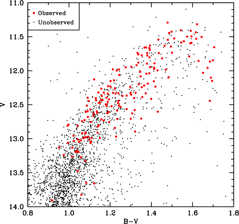
Figure 1: A color–magnitude diagram of the upper RGB for $\omega$ Cen. The large filled circles indicate program stars and the small filled circles are those available from the van Leeuwen et al. (2000) proper motion study.

Target stars, coordinates, photometry, and membership probability were taken from the proper motion study by van Leeuwen et al. (2000). Stars were given priority in the Hydra assignment program based on V magnitude, with a focus on stars in the range 11.0$<$V$<$14.0, which includes all giants in the cluster brighter than the HB up to the RGB tip. Only stars with membership probabilities $\gtrsim$80$\%$ were included for possible study. All observations took place between 2003 July 17 and 2003 July 19. Three different Hydra setups were used with exposure times ranging from 1800 to 3600 seconds. Each setup allowed approximately 100 fibers to be placed on targets, yielding a total initial sample size of nearly 300 stars. At V$\sim$13.5, reaching a signal–to–noise (S/N) ratio of 100 requires 3 hours of total integration time. Unfortunately, weather and time constraints led to one of the setups receiving less than 2 hours of integration time with an average S/N of less than 50. Many of these stars had to be excluded from analysis due to poor S/N; however, the final sample size still includes nearly 200 stars. These are shown in Figure 1 along with the complete sample given in van Leeuwen et al. (2000) for 11.0$<$V$<$14.0.

Due to $\omega$ Cen’s broad RGB, selection effects must be taken into account when interpreting abundance results. Figure 2 shows our observed completion fraction of RGB stars both as a function of V magnitude and B–V color compared to the deeper photometric study by Rey et al. (2004). Since our observing program is biased towards selecting brighter stars, our sample includes more metal–poor than metal–rich stars because metal–rich stars have lower V magnitudes due to H^- opacity increasing with increasing metallicity. While we observed 75$\%$ of all RGB tip stars available, the fraction of stars observed decreases to $\sim$15–50$\%$ in the range 11.5$<$V$<$13.0. Likewise, in considering completeness in B–V color, our sample includes stars of higher luminosity for a given B–V, biasing our results towards the more metal–poor regime.

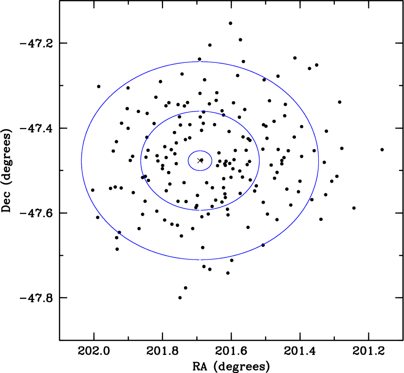
Figure 3: Program stars are shown in terms of position in the field. The cross indicates the field center at 201.691$\arcdeg$, –47.4769$\arcdeg$ (J2000) (13^h26^m45.9^s, –47$\arcdeg$28$\arcmin$37.0$\arcsec$). The ellipses indicate 1, 5, and 10 times the core radius of 1.40$\arcmin$.

Figure 3 shows the location of our observed stars in right ascension and declination relative to the cluster center, defined by van Leeuwen et al. (2000) as 13^h26^m45.9^s, –47$\arcdeg$28$\arcmin$37.0$\arcsec$ (J2000) and marked with a cross in the figure. Since some evidence exists for a correlation between metallicity and distance from the cluster center (Norris et al. 1996; Suntzeff & Kraft 1996; Norris et al. 1997; Hilker & Richtler 2000; Pancino et al. 2000; Rey et al. 2004), we have observed stars as uniformly as possible at radii extending out to $\sim$20$\arcmin$. Near the cluster center, crowding and the physical size of the fibers limited the number of observations inside about 2 core radii, where the core radius is approximately 1.40$\arcmin$ (Harris 1996; rev. 2003 February). We illustrate this effect with the ellipses in Figure 3 that correspond to 1, 5, and 10 core radii.

Basic data reductions were accomplished using the IRAF package ccdproc to trim the bias overscan region and apply bias level corrections. The IRAF task dohydra was employed to correct for scattered light, extract the one–dimensional spectra, remove cosmic rays, apply a flat–field correction, linearize the wavelength scale, and subtract the sky spectrum. Wavelength calibrations were carried out using a high S/N solar sky spectrum because the ThAr lamp was unavailable. Standard IRAF tasks were used to co–add and normalize the spectra. Typical S/N ratios for individual exposures ranged from $\sim$25–50, with co–added spectra having S/N between 75 and 150.

3 RADIAL VELOCITY DETERMINATIONS

$\omega$ Cen’s location in the thick disk (Dinescu et al. 1999) makes field star contamination a more serious problem than for typical halo globular clusters. While we initially only chose targets with high membership probabilities from van Leeuwen et al. (2000), direct measurements of target radial velocities assist with membership confirmation. Radial velocities were determined using the IRAF tasks rvcor, to correct for heliocentric motion, and fxcor, to determine the heliocentric radial velocity. For the comparison spectrum, we used the same high S/N daylight sky spectrum that was used for wavelength calibration. A summary of our determined radial velocities along with membership probabilities from van Leeuwen et al. (2000) are given in Table 2.

The largest radial velocity study of $\omega$ Cen stars to date is by Reijns et al. (2006), who determined radial velocities for $\sim$2,000 RGB stars. Their study finds a strongly peaked distribution near 232 km s^-1, with a median uncertainty of less than 2 km s^-1 and a velocity dispersion of $\sim$6 km s^-1 for the inner 25$\arcmin$ of the cluster. Similarly, Mayor et al. (1997) find $\langle$V_R$\rangle$=232.8 $\pm$ 0.7 km s^-1 ($\sigma$$\sim$17.5 km s^-1) for 471 stars and Suntzeff & Kraft (1996) find $\langle$V_R$\rangle$=234.7 $\pm$ 1.3 km s^-1 ($\sigma$=11.3 km s^-1) for their “bright” sample of 199 stars. Recently, Pancino et al. (2007) determined radial velocities for 650 RGB stars and found $\langle$V_R$\rangle$=233.4 $\pm$ 0.5 km s^-1 ($\sigma$=13.2 km s^-1). We find in agreement with these studies: $\langle$V_R$\rangle$=231.8 km s^-1 $\pm$ 1.6 km s^-1 ($\sigma$=11.6 km s^-1). Our observations do not provide an absolute velocity calibration, but comparison with the other observations of the average velocity of cluster stars suggests that the systematic error of our radial velocities is less than about 2 km s^-1. Since all of our stars listed in Table 2 are less than 3$\sigma$ away from the cluster averaged velocity and $\omega$ Cen’s velocity is high relative to the general field population, it is unlikely any of our targets are field stars.

4 Analysis

We have derived Fe and Al abundances using lines available in the spectral range 6500–6750 Å with either equivalent width or synthetic spectrum analyses. Spectrum synthesis was used to determine Al abundances in metal–rich and/or CN–strong stars. When multiple lines were available, the stated abundances represent the average of the individual lines. Effective temperatures (T_eff) and gravities (log g) were estimated using published (V–K)₀ photometry. T_eff and microturbulence (V_t) were further refined via spectroscopic analyses. The analysis follows the methods described in Johnson et al. (2005) and Johnson & Pilachowski (2006).

4.1 Model Stellar Atmospheres

Using V photometry from van Leeuwen et al. (2000) and K_s photometry from 2MASS, we estimated T_eff with the color–temperature relation described in Alonso et al. (1999; 2001), which is based on the infrared flux method (Blackwell & Shallis 1977). However, the Alonso et al. (1999) method requires the photometry to be on the Carlos Sánchez Telescope (TCS) photometric system. We transformed the V and K_s magnitudes onto the TCS system using the transformations provided in Alonso et al. (1994; 1998) and Carpenter (2001), as summarized in Johnson et al. (2005). To correct for interstellar reddening and extinction, we applied the correction recommended by Harris (1996; rev. 2003 February) of E(B–V)=0.12 and used E(V–K)/E(B–V)=2.7 (Johnson 1965). While Calamida et al. (2005) claim differential reddening, perhaps differing by as much as a factor of two near the core, could be a problem, the well defined evolutionary sequences seen in Villanova et al. (2007) seem to indicate it is not too severe. Van Loon et al. (2007) find some evidence for interstellar absorption by gas in the cluster, but this is concentrated near the core where our observations are sparse. Therefore, we have only applied a uniform reddening correction. Bolometric corrections were applied using the empirical relations given in Alonso et al. (1999) assuming a distance modulus of (m–M)_V=13.7 (van de Ven et al. 2006).

Applying the proper color–temperature relation requires knowledge of a star’s metallicity. Therefore, we took the empirical relation given in van Leeuwen et al. (2000; their eq. 15), which gives [Ca/H] as a function of V and B–V, and assumed [Ca/Fe]$\sim$+0.30 for [Fe/H]$\lesssim$–1.0 (e.g., Norris & Da Costa 1995), with a linear decrease towards [Ca/Fe]=0.0 at [Fe/H]=0.0. This gave a rough estimate of [Fe/H] for each star and allowed us to choose the proper equation in Alonso et al. (1999).

Since only one Fe II line was available for analysis (6516 Å), we determined surface gravity using the standard relation,

$$log(g)=0.40(M_{bol.}-M_{bol.\sun})+log(g_{\sun})+4(log(T/T_{\sun}))+log(M/M_{\sun}),$$ (1)

instead of the ionization equilibrium of Fe. We assumed M=0.80 M_☉ for all stars, regardless of metallicity. Though there may be an intrinsic age spread of a few Gyr on the RGB (see $\S$5 for further discussion on this issue), this will lead to a mass difference only of order $\sim$0.05 M_☉, which is negligible for surface gravity determinations.

In addition to T_eff, log g, and [Fe/H] estimates, we also needed a starting point with V_t. Initial estimates were based on the empirical relation derived in Pilachowski et al. (1996), which gives V_t as a function of T_eff for metal–poor field giants and subgiants. Typical V_t values ranged from about 1.3–2.3 km s^-1 in the temperature range 5000–3800 K, respectively.

We generated the model stellar atmospheres by interpolating in the ATLAS9 (Castelli et al. 1997) grid of models without convective overshoot. Initial models were created using the T_eff, log g, [Fe/H], and V_t estimates as described above. T_eff was further refined by removing trends in Fe abundance as a function of excitation potential. Likewise, V_t was improved by removing trends in Fe abundance as a function of reduced width (log(EW/$\lambda$)). A comparison between photometric and spectroscopically determined temperatures is given in the top panel of Figure 4. Typical photometric and spectroscopic temperature estimates agree to within approximately $\pm$100 K. The bottom panel of Figure 4 shows our spectroscopically determined V_t as a function of T_eff for different metallicity bins with a linear least squares fit given by,

$$V_{\rm t}=-0.0011(T_{\rm eff})+6.66,$$ (2)

which is independent of metallicity. This fit agrees to within $\sim$0.10–0.15 km s^-1 to that given in Pilachowski et al. (1996). Figure 5 shows our derived [Fe II/H] given as a function of [Fe/H]. As stated above, we only had one Fe II line available for analysis, but the fact that both Fe estimates agree to within 0.16 dex on average ($\sigma$=0.12 dex) leads us to believe our surface gravity estimates are not in serious error. A complete list of our adopted model atmosphere parameters is provided in Table 3.

4.2 Derivation of Abundances

Abundances were determined using equivalent width analyses for all Fe lines and most Al lines, with the exception of cases where evidence for considerable CN contamination near the 6696, 6698 Å Al doublet (i.e., metal–rich and/or CN–strong stars) existed and spectrum synthesis was used instead. We measured equivalent widths using a FORTRAN program developed for this project that interactively fits a Gaussian curve to each absorption line by implementing a Levenberg-Marquardt algorithm (Press et al. 1992) to find the least–squares fit given a continuum level and limits of integration. A high resolution, high S/N Arcturus spectrum was simultaneously overplotted for each spectrum to aide in continuum placement and line identification. The program also has the ability to fit up to five Gaussians simultaneously for deblending purposes; however, all equivalent widths were verified independently using IRAF’s splot package.

4.2.1 Equivalent Width Analysis

Final abundances were calculated using the abfind driver in the 2002 version of the local thermodynamic equilibrium line analysis code MOOG (Sneden 1973). Adopted log gf values are the same as those employed in Johnson et al. (2006), which were adapted from line lists provided in Thévenin (1990), Sneden et al. (2004; modified from Ivans et al. 2001), and Cohen & Meléndez (2005). A summary of our line list is given in Table 4 and the measured equivalent widths are provided in Table 5.

While we had identified 20 Fe I lines for analysis, in most cases only 10–15 lines could be used due to severe line blending, bad ccd pixels, or line strength. In this sense, only lines lying on the linear part of the curve of growth were used, which meant neglecting almost all lines with a reduced width larger than about –4.5 (roughly 200 mÅ at 6600 Å). This unfortunately meant that many lines in metal–rich stars are too strong to give accurate abundances using our techniques. For the cases where Al abundances were determined using equivalent width measurements, weak line blends were taken into account using deblending methods. As stated above, stars with strong line blending or molecular line blanketing in the region near the Al doublet were analyzed with spectrum synthesis.

Typical uncertainties are quite small for [Fe/H] determinations with internal line–to–line spreads of $\sim$0.10–0.15 dex and $\sigma$/$\sqrt{N}$ $<$ 0.05 dex on average. Sample spectra for stars of approximately the same T_eff but different metallicities are shown in Figure 6. Here we illustrate that our [Fe/H] determinations are at the very least consistent in a relative sense as one notices the increasing Fe line strengths and CN–band strengths with increasing metallicity. The uncertainty in Al abundances is larger given that only two lines are available, but the two lines give a remarkably consistent abundance, with an average $\sigma$/$\sqrt{N}$=0.08 dex. It should be noted that in several of our spectra only one Al line could be confidently measured due mostly to bad pixels. In Figure 6, the reader can see the stark contrast in line strength between a star such as 51021, which has [Al/Fe]=+0.15 at [Fe/H]=–1.44, and star 61085, which has [Al/Fe]=+0.97 at [Fe/H]=–1.15. A summary of all derived abundances and associated $\sigma$/$\sqrt{N}$ values is given in Table 6.

4.2.2 Spectrum Synthesis Analysis

As mentioned above, we determined Al abundances for metal–rich and/or CN–strong stars using the synth driver in MOOG. Candidates for spectrum synthesis were chosen based on visual inspection of the 6680–6700 Å region, where the majority of lines surrounding the Al doublet are CN lines. Stars where CN contamination was seen between the Al lines were designated for synthetic spectrum analysis (e.g., see Figure 6, lower two spectra).

The atomic line list (with the exception of the two Al lines) was taken from the Kurucz atomic line database. We adjusted the oscillator strengths from this line list so the line strengths matched those in the solar spectrum. For the CN molecular line list, we used a combination of one available from Kurucz and one provided by Bertrand Plez (2007, private communication; for a description on how the line list was prepared, see Hill et al. 2002).

Since most of the program stars do not have known C, N, or ¹²C/¹³C abundances, we started with [C/Fe]=–0.5, [N/Fe]=+1.5, and ¹²C/¹³C=5, values roughly consistent with previous work (e.g., Norris & Da Costa 1995; Smith et al. 2002). We then treated the nitrogen abundance as a free parameter and adjusted it until a satisfactory fit was achieved. Typical best fit [N/Fe] values were $\sim$+1.0 to +1.5. To test the effect of different ¹²C/¹³C ratios, we generated two sets of spectra with ¹²C/¹³C=5 and ¹²C/¹³C=1000. The fits to the CN lines were indistinguishable between the two cases, meaning ¹²C is the dominant isotope in this spectral region and thus synthesized CN lines are insensitive to the ¹³C abundance.

With the CN lines fit, we were then able to adjust the Al abundance until the synthetic spectrum matched the observed. Sample synthesis fits are given in Figure 7 for a metal–poor and metal–rich case. Aside from the CN lines, the Fe I line near the 6696 Å feature is the only other contaminating line in the region, but this line has an excitation potential of nearly 5 eV, making its contribution mostly negligible in these cool stars. Generally, the abundances given by the 6696 and 6698 Å lines agreed to within about $\pm$0.10 dex. Since a significant percentage of our Al abundances were determined using synthesis analyses, we tested for systematic offsets between synthesis and equivalent width methods. For sample stars that were both metal–poor and did not show signs of CN contamination, the difference in [Al/Fe] determined via both methods was less than 0.05 dex. However, for higher metallicity stars and those with possible CN contamination, the difference was 0.10–0.20 dex, with equivalent width analyses always overestimating the abundance. The quoted values for Al abundances derived via spectrum synthesis are given as the average from those two lines. A summary of our derived abundances is given in Table 6. Stars with Al determinations via synthesis are designated by “Syn” in the 6696 and 6698 Å columns of Table 5.

4.2.3 Abundance Sensitivity to Model Atmosphere Parameters

We tested the effects on derived abundances from changes in model atmosphere parameters by altering T_eff $\pm$ 100 K, log g $\pm$ 0.25 cm s^-2, and V_t $\pm$ 0.25 km s^-1 for models of [Fe/H]=–2.0, –1.5, and –1.0. As can be seen in Table 7, T_eff uncertainties are the primary source of error for Fe I and Al I, and surface gravity is the primary source for Fe II abundances. This seems logical given that Fe I and Al I reside in a subordinate ionization state, and Fe II exists in the primary ionization state.

Following Table 7, an uncertainty of order 100 K in T_eff leads to an error of $\sim$0.10–0.20 dex in Fe I, though the effect is somewhat reduced at higher metallicity. The opposite is true for Fe estimates based solely on the Fe II line, where the error range is $\sim$0.05–0.10 dex and the uncertainty becomes larger with increasing metallicity. Though the variation in Al I abundance as a function of T_eff uncertainty is smaller than for Fe I, it is still of order 0.10 dex with a weak dependence on metallicity.

The effects of surface gravity uncertainty are of order 0.10 dex for the Fe II line, but are negligible for the neutral Fe and Al lines. For this reason, enforcing ionization equilibrium between different species is often used for constraining surface gravity estimates. As mentioned in $\S$4.2.1, having only one Fe II line means the Fe abundance derived from Fe II is probably no more accurate than the typical line–to–line scatter present in Fe I ($\sigma$$\sim$0.10–0.15 dex). Combined with the sensitivity of Fe II to surface gravity estimates of order $\pm$0.25 cm s^-2, the fact that agreement between Fe I and Fe II is better than about 0.10 dex (see Figure 5) suggests estimates based on evolutionary arguments provide a decent approximation to the surface gravity; however, Table 7 shows this has little effect on our derived Fe I and Al I abundances. From this, we can safely assume that contamination from AGB stars, which have M$\sim$0.60 M_☉ and thus a lower surface gravity, will not significantly alter our results.

The ad hoc microturbulence parameter, adjusted to remove abundance trends as a function of reduced width, has the strongest effect for lines lying on the flat part of the curve of growth. As is seen in Table 7, the effect on the Fe I abundance due to uncertainty in V_t increases with increasing metallicity because the lines become progressively stronger. However, Fe II and Al I are mostly unaffected due to their relatively small equivalent widths and the effect on Fe I is still $<$0.10 dex even at [Fe/H]=–1.0.

In addition to variations in model stellar atmosphere parameters we tested the sensitivity of Al abundance to CN strength via spectrum synthesis by varying [N/Fe]$\pm$0.30 dex. Changing the nitrogen abundance by this amount worsens the fit to the CN lines in the spectrum, but alters the derived [Al/Fe] abundance less than 0.10 dex at all metallicities. Note that since [O/Fe] is unknown for most of our program stars and [O/Fe] can have values ranging from about +0.30 to less than –0.50, it is not possible to constrain the molecular equilibrium equations to derive true [C/Fe] and [N/Fe]. We present the [Al/Fe] results for each metallicity bin in Table 7.

4.3 Comparison with the Literature

While $\omega$ Cen has been the subject of multiple abundance studies (see $\S$ 1 for a brief review), most of these are low resolution studies that do not involve elements other than Fe and/or Ca. Therefore, we are only comparing results in the literature for which moderate to high resolution Al data are available and with which we have three or more stars in common. This limits the comparison to Brown & Wallerstein (1993; 3 stars), Norris & Da Costa (1995; 24 stars), Zucker et al. (1996; 4 stars), and Smith et al. (2000; 3 stars).

In Figure 8, we present the values of T_eff, log g, [Fe/H], and V_t given in the literature versus those obtained in this study. As can be seen from the figure, agreement is quite good for the temperature and surface gravity estimates, with the scatter increasing slightly for the metallicity and microturbulence estimates. For T_eff, the average offset between our study and the literature is –7 K ($\sigma$$\sim$50 K), and the average difference for log g is –0.02 cm s^-2 ($\sigma$$\sim$0.10 cm s^-2). This indicates that any disagreement between literature Fe and Al abundances and ours is not due to choices of T_eff and log g. Similarly, [Fe/H] measurements agree to within 0.02 dex on average ($\sigma$$\sim$0.20 dex). The reason for the larger dispersion in microturbulence estimates is not entirely clear, but it could be due to factors such as the number of lines available, data quality, continuum placement, and type of lines used (i.e., high and/or low excitation potential). However, on average the agreement is within 0.10 km s^-1 ($\sigma$$\sim$0.25 km s^-1).

Comparison between our derived [Al/Fe] abundances versus those in the literature are provided in Figure 9. Given the various data qualities, choices of model atmospheres and parameters, and adopted atomic line data, agreement is again quite good. The average offset between our derived abundances and those available in the literature is 0.06 dex ($\sigma$$\sim$0.30 dex). Given that typical uncertainties in [Al/Fe] are of order 0.10–0.20 dex, agreement is comparable to that range.

5 RESULTS AND DISCUSSION

5.1 Fe Abundances

As discussed in $\S$1, it has been known for many years and shown by several authors that $\omega$ Cen has a considerable spread in metallicity that ranges from slightly less than [Fe/H]=–2.0 to more than [Fe/H]=–0.7. While several lower resolution spectroscopic (Norris et al. 1996; Suntzeff & Kraft 1996; Sollima et al. 2005b; Kayser et al. 2006; Stanford et al. 2006; Stanford et al. 2007; van Loon et al. 2007; Villanova et al. 2007) and photometric (Lee et al. 1999; Hilker & Richtler 2000; Hughes & Wallerstein 2000; Pancino et al. 2000; van Leeuwen et al. 2000; Rey et al. 2004; Stanford et al. 2004; Sollima et al. 2005a; Stanford et al. 2006) studies have obtained metallicity estimates for a large number of stars (N$\gtrsim$500 in some cases), there have only been a few high resolution spectroscopic studies with a significant number (N$\gtrsim$10) of stars observed (Norris & Da Costa 1995; Smith et al. 2000; Piotto et al. 2005; Sollima et al. 2006). However, aside from the present study, Norris & Da Costa (1995) still represents the largest (N=40) single high resolution analysis of $\omega$ Cen RGB stars. The general results from the metallicity studies can be summarized as: (1) few stars exist at [Fe/H]$<$–2.0, (2) a primary peak in the metallicity distribution is observed at [Fe/H]$\sim$–1.8 to –1.6, (3) there is a long tail of increasing metallicity up to [Fe/H]$\sim$–0.5, and (4) there appear to be multiple peaks in the distribution at various [Fe/H] values.

In Figure 10, we present a histogram of our derived metallicity distribution function for all 180 stars. We find in agreement with previous studies that there are at least four distinct populations with the most metal–poor having [Fe/H]$\sim$–1.75, the two intermediate metallicity populations have [Fe/H]$\sim$–1.45 and –1.05, and the most metal–rich population has [Fe/H]$\sim$–0.75. While our observations are skewed towards observing more metal–poor stars (see Figure 2), there are intrinsically more metal–poor than metal–rich stars, as can be seen in Figure 1. This means our derived metallicity distribution is affected by both the actual distribution and observational selection effects. Given that we only observed one star on the most metal–rich branch, it is possible that stars with metallicities higher than [Fe/H]=–0.75 exist. However, since our observed completion fraction is significantly higher for the most metal–poor stars, it is likely that our observed distribution function is accurate in a relative sense such that the cluster was rapidly enriched from the primordial metallicity of [Fe/H]$\sim$–2.15 to the first major epoch of star formation at [Fe/H]$\sim$–1.75. The absence of stars more metal–poor than [Fe/H]$\sim$–2.2 means the proto–$\omega$ Cen environment was already pre–enriched, perhaps from processes such as cloud–cloud collisions (Tsujimoto et al. 2003), when the primary metal–poor population formed. In contrast, field stars in the Galactic halo exhibit a wide range of metallicities from [Fe/H]$>$0.0 to [Fe/H]$<$–4.0 (e.g., Gratton et al. 2004), indicating that the two do not share a common chemical enrichment history.

The distribution shown in Figure 10 suggests that if $\omega$ Cen evolved as a single entity (i.e., without significant contributions from mergers), then there were four to five significant star formation episodes that occurred. This seems to fit the high resolution photometric data from Sollima et al. (2005a) and Villanova et al. (2007) that show the multiple giant branches appear in discrete groups instead of as a continuous distribution. This trend is similarly reproduced in Figure 11, where our derived metallicities are superimposed on the photometric data from van Leeuwen et al. (2000). Here, even when binning by the approximate 3$\sigma$ value of each peak in the distribution from Figure 10 (0.3 dex), the different metallicity groups can be separated. The metallicity distribution from Figure 10 is very well produced in the hydrodynamical chemical enrichment simulations of Marcolini et al. (2007), where they assumed $\omega$ Cen is the core remnant of a dwarf spheroidal galaxy that was captured and tidally stripped $\sim$10 Gyr ago with star formation occurring over roughly 1.5 Gyr. The simulated metallicity peaks from Marcolini et al. (2007) lie at [Fe/H]$\sim$–1.6, –1.35, –1.0, and –0.70, which are very similar to ours at [Fe/H]=–1.75, –1.45, –1.05, and –0.75.

There is some evidence that different metallicity populations may be spatially and kinematically unique (Norris et al. 1996; 1997; Suntzeff & Kraft 1996; Hilker & Richtler 2000; Pancino et al. 2000; 2003). In Figure 12, we present Fe and Al abundances as a function of distance from the cluster center. Keeping in mind our observational bias, we find a marginal tendency for the more metal–rich stars to be located in the inner regions of the cluster while the more metal–poor stars are rather evenly distributed at all radii sampled here. However, given our small sample size in the metal–rich regime, we are unable to make any definitive arguments for or against a metallicity–radius relationship. It should be noted though that Ikuta & Arimoto (2000) and Rey et al. (2004) do not find any strong evidence for the metal–poor and metal–rich populations having a spatially different structure. Even though the relaxation time for $\omega$ Cen is thought to exceed 5 Gyr (Djorgovski 1993; Merritt et al. 1997), any correlation between projected spatial position and metallicity is apparently subtle. However, it has been pointed out in deep photometric surveys (e.g., Rey et al. 2004) that the most metal–rich RGB–a is predominately seen in CMDs of the inner region of the cluster.

The main result indicating that at least the most metal–rich population may have a different formation history is that those stars appear to have a lower velocity dispersion (i.e. are kinematically cooler) than the other populations and do not show signs of rotation (Norris et al. 1997). In Figure 13 we show our derived radial velocities plotted both as a function of log $\epsilon$(Fe) and log $\epsilon$(Al), where the error bars indicate the velocity dispersion in the data. To within one standard deviation, we do not find significant evidence for any of the stellar populations having a different bulk radial velocity or velocity dispersion. It seems unlikely that a larger sample size would provide significantly different results because Reijns et al. (2006) determined radial velocities for nearly 2000 $\omega$ Cen members and concluded the RGB–a stars had radial velocity and dispersion values consistent with the entire cluster. Pancino et al. (2007) have shown the rotational velocities for all populations are comparable to one another, but interestingly they find an underlying sinusoidal pattern in their measured velocities as a function of position angle. However, the metal–poor, intermediate metallicity, and anomalous giant branches all show the same sinusoidal pattern. Whether any true kinematic anomaly exists for this cluster or not remains to be seen.

5.2 Al Abundances

The bulk of aluminum production in galaxies and globular clusters is thought to arise from quiescent carbon and neon burning in massive stars (M$\gtrsim$8 M_☉) and HBB occurring in the envelopes of IM–AGB stars via the MgAl cycle (e.g., Arnett & Truran 1969; Arnett 1971). In most Galactic globular clusters, there is a very small ($<$0.10 dex) spread in the abundance of heavy $\alpha$ and Fe–peak elements, with a somewhat larger spread ($\sim$0.3–0.6 dex) in s– and r–process elements (e.g., Sneden et al. 2000). However, the lighter elements carbon through aluminum are typically not uniform and in some cases show star–to–star variations of more than a factor of 10. While $\omega$ Cen does not share all of the same chemical characteristics as globular clusters, the primary production locations of each element should be similar to globular clusters and/or the Galactic halo. The lesson learned from the monometallicity of “normal” globular clusters is that however Al manifests itself onto the surface of stars, the process must not alter Fe–peak, s–process, or r–process abundance ratios. This means that the often large star–to–star variation of [Al/Fe] seen in globular clusters (but not in halo field stars) are not due to supernova yields or the s–process, leaving either in situ deep mixing or HBB as the possible sites for [Al/Fe] variation. With these two scenarios in mind, we explore Al abundances with the goal of helping to constrain the source of Al variation and chemical evolution in $\omega$ Cen.

While the literature on Fe abundances for both evolved and main sequence stars is quite extensive, the spectroscopic surveys by Norris & Da Costa (1995) and Smith et al. (2000) represent the only studies to consider light element abundances that include Al for a large (N$\geq$10) number of RGB stars in $\omega$ Cen. The results of those two studies indicate that the full range of [Al/Fe] is larger than 1.0 dex, Al and Na are correlated, Al and O are anticorrelated, and there is a hint of a decrease in [Al/Fe] with increasing [Fe/H]. We present the results of our larger sample plotting [Al/Fe] as a function of [Fe/H] in Figure 14. Even for the lowest metallicity stars, a large range in [Al/Fe] of $\sim$0.70 dex is already present. Near the first metallicity peak at [Fe/H]=–1.75, where it is assumed the first episode of star formation after the initial enrichment period occurred, the full range in [Al/Fe] reaches a maximum value of $\sim$1.3 dex. This star–to–star variation remains mostly constant until about [Fe/H]=–1.4, where the variation begins to decrease smoothly with increasing [Fe/H]. Interestingly, the “floor” Al abundance remains mostly constant at [Al/Fe]$\sim$+0.15, regardless of the star’s metallicity; a characteristic shared with many globular clusters of various metallicity and in agreement with [Al/Fe] values typical of Galactic halo stars in $\omega$ Cen’s metallicity regime.

In Figure 15, we overlay a boxplot on top of the underlying distribution from Figure 14. The median [Al/Fe] ratio typically resides between about 0.45 and 0.80 dex for all well–sampled metallicities, with a relatively constant interquartile range. This implies that the average amount of Al in the cluster must increase with increasing Fe abundance, at least up to [Fe/H]$\sim$–1.4. This result is confirmed in Figure 16, where log $\epsilon$(Al) is plotted against log $\epsilon$(Fe). It appears that for metallicities higher than about log $\epsilon$(Fe)=6.0 ([Fe/H]$\approx$–1.50), log $\epsilon$(Al) no longer increases beyond log $\epsilon$(Al)$\approx$6.40 and the star–to–star scatter decreases. This result is likely robust against our observational bias because all stars observed in the metal–rich regime are located at or near the RGB tip (see Figure 1), where it is believed any Al enhancements due to deep mixing should be the most apparent. However, no obvious trend is seen between Al abundance and evolutionary state.

As discussed previously, there is some evidence for a correlation between Fe abundance and distance from the cluster center and we show the results from this study in the bottom panel of Figure 12. In the top panel of Figure 12, we present the same data but for Al instead of Fe. While there may be a tendency for the most metal–rich stars to be located inwards of about 10–15$\arcmin$, there is no evidence of a trend for Al. Instead, stars of varying Al abundance are uniformly spread throughout the entire region sampled, at least out to $\sim$20$\arcmin$. Likewise, the top panel of Figure 13 shows average radial velocities for Al abundances in 0.10 dex bins. To within uncertainties, there appears to be no trend in either radial velocity or velocity dispersion with log $\epsilon$(Al). The fact that we do not find any preference of Al abundance or star–to–star dispersion with distance from the cluster center or radial velocity suggests star formation occurred on timescales shorter than those required to uniformly mix the gas.

5.3 Possible Implications on Chemical Evolution

From our available spectroscopic data for 180 RGB stars, we have confirmed the existence of at least four stellar populations ranging in metallicity from –2.2$<$[Fe/H]$<$–0.70, in agreement with previous photometric, low resolution spectroscopic, and smaller sample high resolution spectroscopic studies. Additionally, we have determined [Al/Fe] abundances for about 165 giants, most of which for the first time, with a sample larger by more than a factor of four than what was previously available in the literature. We find a constant Al abundance floor of [Al/Fe]$\sim$+0.15 present at all metallicities, but with a largely varying and metallicity dependent spread above the floor. The star–to–star variation reaches a maximum extent in the intermediate metallicity regime, which is consistent with the second peak in the metallicity distribution, and begins to decline at higher metallicities. The floor itself is consistent with observations of field stars and is predicted by Galactic chemical evolution models, but the large [Al/Fe] variations are not predicted. Observations of some Galactic globular cluster stars, especially more metal–poor than [Fe/H]$\sim$–1.5, show similar large star–to–star variations in [Al/Fe]. Combining our determined Fe and Al abundances with those available in the literature for these and other elements now allows us to examine each metallicity regime in turn.

5.3.1 The Metal–Poor Population

A prominent feature of the metal–poor stars ([Fe/H]$\lesssim$–1.6) in $\omega$ Cen is the rapidly increasing abundances of Na, Al, and light and heavy s–process elements relative to Fe as the metallicity increases from [Fe/H]=–2.2 to the first metallicity peak at [Fe/H]=–1.75 (e.g., Norris & Da Costa 1995; Smith et al. 2000). These increases are accompanied by nearly constant heavy [$\alpha$/Fe]$\sim$+0.30, low Cu abundances ([Cu/Fe]$\sim$–0.60), and low r–process abundances ([Eu/Fe]$\sim$–0.50). These results seem to indicate that massive stars exploding as type II SNe are the primary contributors for Fe–peak and heavy $\alpha$–element enhancement in the cluster, but the low Eu abundances, which should be synthesized in the same stars, are puzzling. Additionally, the growing s–process component appears to be best fit by models of 1.5–3 M_☉ AGB ejecta (Smith et al. 2000). The lack of clear evidence for type Ia SNe having contributed to the chemical composition of metal–poor stars in $\omega$ Cen (e.g., Smith et al. 2000; Cunha et al. 2002; Pancino et al. 2002; Platais et al. 2003) is consistent with the $\gtrsim$1 Gyr timescales needed for type Ia SNe to evolve and the fact that they might not efficiently form in metal–poor environments (Kobayashi et al. 1998).

As mentioned above, the majority of Al present in the atmospheres of these RGB stars was likely produced in type II SNe explosions that polluted the pristine gas from which these stars formed. While the heavy element data do not support high mass ($\gtrsim$8M_☉) stars being the source for the more than 1.0 dex [Al/Fe] variations, that may be explained from HBB occurring in IM–AGB stars, in situ deep mixing, or a hybrid scenario. In Figures 14–16, we have shown that [Al/Fe]$\geq$0 for all metal–poor stars sampled, but a constant Al abundance floor is setup at [Al/Fe]$\sim$+0.15 with a rapidly increasing star–to–star dispersion that reaches about 1.3 dex in extent by [Fe/H]=–1.75. For the neutron capture elements, which are the only other group exhibiting a variations with metallicity, Smith et al. (2000) showed stars with [Fe/H]$\sim$–2 are dominated by an r–process component with a shift to a primarily s–process component by [Fe/H]$\gtrsim$–1.8.

In the pure pollution scenario, which does not invoke deep mixing affecting elements heavier than N, type II SNe, low and IM–AGB stars, and perhaps winds from less evolved very massive stars (e.g., Maeder & Meynet 2006) are responsible for all abundance anomalies. Adding our large Al data set to the sample of stars previously observed may help constrain enrichment timescales and polluting AGB masses. Conventional theory suggests light and s–process elements do not share the same origin and $\omega$ Cen’s s–process component is best fit with lower mass AGB stars, but masses lower than $\sim$3–4 M_☉ undergo third dredgeup without significant HBB (e.g., Karakas & Lattanzio 2007) and thus should not appreciably alter their envelope Al abundances. Additionally, Ventura & D’Antona (2007) suggest globular cluster light element anomalies can only be explained with ejecta from AGB stars in the mass range of $\sim$5–6.5 M_☉. While our sample only includes two stars with [Fe/H]$<$–2 (36036 & 51091), the elevated [Al/Fe] ratios of +0.40 and +1.13 suggest IM–AGB stars, with lifetimes of about 50–150$\times$10⁶ yrs (Schaller et al. 1992), have already polluted the $\omega$ Cen system. In this case, the low metallicity environment would favor high [Al/Fe] yields from HBB processes occurring in IM–AGB stars. The rapidly rising average value of log $\epsilon$(Al) shown in Figure 16 in the metallicity regime –2.0$\lesssim$[Fe/H]$\lesssim$–1.6 implies a continued contribution from IM–AGB stars, presumably forming from the same star formation event that creates the first peak in the metallicity distribution. The top two panels of Figure 17 show binned [Al/Fe] for this metallicity regime and we note approximately four sub–populations with [Al/Fe]$\sim$+0.15, +0.45, +0.85, and $>$+1.05. Predicted yields from type II SNe (e.g., Woosley & Weaver 1995) and measurements of field stars (e.g., Fulbright 2000) suggest type II SNe should enrich the ISM with [Al/Fe]$\sim$+0.10 to +0.30 while $\sim$5–6.5 M_☉ AGB stars should produce [Al/Fe]$\sim$+0.50 to +1.10 (e.g., D’Antona & Ventura 2007), which could explain our observed distribution. Given the rather short lifetimes of stars believed to produce Al and the fact that evidence for 1.5–3.0 M_☉ pollution does not appear until [Fe/H]$\sim$–1.8, it would seem that $\omega$ Cen was probably enriched from [Fe/H]=–2.2 to –1.75 in $\sim$0.5–1.0 Gyr.

5.3.2 The Intermediate Metallicity Populations

For the two intermediate metallicity populations ([Fe/H]=–1.45 and [Fe/H]=–1.05), the heavy [$\alpha$/Fe] ratio remains constant and the s–process abundances level off with very little star–to–star dispersion (Norris & Da Costa 1995; Smith et al. 2000). As in the most metal–poor stars, r–process and Cu ratios relative to Fe remain low and mostly unchanged. However, the star–to–star scatter in O, Na, and Al is still quite large. It is interesting to point out that log $\epsilon$(Al) reaches its maximum value at about the same metallicity at which the s–process elements reach a constant ratio relative to Fe. The [Al/Fe] abundance floor is constant throughout this metallicity regime at [Al/Fe]$\sim$+0.15, which means the scatter, still considerably larger than for [Ba/Fe], decreases as a function of increasing metallicity. This trend should presumably be present for Na and in the opposite sense for O assuming the Na–Al correlation and O–Al anticorrelation exist at all metallicities.

Had the scatter in Al abundances been comparable to that of other heavier elements in this metallicity range ($\sim$0.10–0.30 dex) with a nearly constant [Al/Fe] ratio, as is seen in field stars, we might be inclined to believe Al enhancement in the cluster was due solely to production in massive stars and that typical type II SNe ejecta have [Al/Fe]$\sim$+0.15. It is interesting to note that the [Al/Fe] floor tracks closely (with a slight offset of $\sim$0.2-0.3 dex) to the Galactic chemical evolution model presented in Timmes et al. (1995; their Figure 19), assuming the amount of Fe ejected is decreased by a factor of two, and Samland (1998; their Figure 10), with an increase in secondary (i.e., metal–dependent) Al production by a factor of five. If the well–known light element correlations/anticorrelations seen in previously observed $\omega$ Cen stars (e.g., Norris & Da Costa 1995) holds at all metallicities and for all stars, those with [Al/Fe]$\sim$+0.15 should also have [O/Fe]$\sim$+0.30, heavy [$\alpha$/Fe]$\sim$+0.30, and [Na/Fe]$\sim$–0.20, which are consistent with predicted yields from type II SNe (e.g., Woosley & Weaver 1995). It could be that these stars formed preferentially out of SNe ejecta without significant IM–AGB contamination.

While the maximum observed log $\epsilon$(Al) increases with metallicity for the most metal–poor $\omega$ Cen giants, this trend halts at [Fe/H]$\sim$–1.4, which coincides with the second peak in the metallicity distribution (i.e., the next round of star formation). We know the heavy [$\alpha$/Fe], [Ba/Fe], and floor [Al/Fe] ratios remain constant at higher metallicities, indicating an increase in log $\epsilon$(Ba), log $\epsilon$($\alpha$), and the minimum log $\epsilon$(Al) that track with Fe. The question now posed by the Al data is why does the process producing the high Al values shut off or become less efficient at [Fe/H]$\gtrsim$–1.45? Increases in metallicity lead to lower temperatures at the bottom of the convective envelope and require higher masses for HBB to occur. It may be that we are observing the result of lower convective efficiency at higher metallicity and/or that fewer IM stars form in higher metallicity environment. IM–AGB models in the metallicity range of –1.5$\lesssim$[Fe/H]$\lesssim$–0.7 (e.g., Fenner et al. 2004; Ventura & D’Antona 2007; 2008) predict [Al/Fe] yields of $\sim$+0.5 to +1.0, with lower [Al/Fe] yields at higher [Fe/H]. This may explain the bimodal distribution in the bottom panels of Figure 17, with the abundances in between possibly being due to varying degrees of ejecta dilution. The fact that the metallicity at which the heavy elements cease to increase in abundance more quickly than Fe and the metallicity where the maximum [Al/Fe] begins to decrease coincide suggests an important parameter changed in $\omega$ Cen at this point in its evolution. It may even be the case that this is when the progenitor dwarf galaxy began to change structurally via encounters with the Galactic disk. It appears that at metallicities higher than [Fe/H]=–1.45, the cluster slowly approaches a constant [Al/Fe], which is consistent with values observed in the halo.

While type Ia ejecta have been mostly ruled out by previous studies as contributors to the most metal–poor population, the metallicity at which they become important contributors is unclear. Marcolini et al. (2007) claim that their intermediate metallicity peak at [Fe/H]$\sim$–1.4 is due primarily to inhomogeneous pollution by type Ia SNe. It is interesting to note that in this same metallicity bin we find a median [Al/Fe] value about 0.40 dex lower than the two surrounding bins as well as the only star with [Al/Fe]$\lesssim$+0.15. It is uncertain whether this is a real effect or simply due to an anomalous selection of stars. Inhomogeneous pollution by type Ia SNe may also explain the bimodal distribution seen in the bottom panels of Figure 17 where stars polluted by both type Ia ejecta and IM–AGB stars exhibit lower [Al/Fe] ratios and “normal” stars polluted by type II SNe and IM–AGB stars have higher [Al/Fe] values. While the same trend is not particularly apparent for s–process elements (e.g., Smith et al. 2000), this may be due to a smaller sample size, especially if inhomogeneous pollution only affected a small percentage of intermediate metallicity stars; however, this could explain the few observations in the literature of stars with [Fe/H]$\sim$–1.4 and [Ba/Fe]$\sim$0 (e.g., Smith et al. 1995).

5.3.3 The Metal–Rich Population

For stars more metal–rich than [Fe/H]$\sim$–1, there is some evidence of a decrease in [$\alpha$/Fe] and an increase in [Cu/Fe] (Pancino et al. 2002; but see also Cunha et al. 2002), which, if true, likely indicates an increased contribution from type Ia SNe. Similarly, there appears to be a decrease in [Eu/Fe] with perhaps a similar decrease in the abundance of s–process elements relative to Fe (Norris & Da Costa; Smith et al. 2000). Although the Al data are rather incomplete in this metallicity regime, the general trends seen in slightly more metal–poor stars appear to continue.

While the scope of an age spread amongst the various metallicity populations is still unknown, the Al data presented here seem to indicate that the age difference between the intermediate and metal–rich populations is not especially large. In particular, stars with the largest values of log $\epsilon$(Al) appear with [Fe/H] ranging from –1.5 to –0.7, perhaps indicating that they formed from gas polluted by the same generation of IM–AGB ejecta. In this scenario, the lower [Al/Fe] ratios at high metallicity might be due to those stars forming in regions where [Fe/H] increased due to inhomogeneous pollution by type Ia SNe, as mentioned in Marcolini et al. (2007). In their scenario, this effect should be more important for the inner regions of the cluster. This may be corroborated by our finding that there is no apparent relationship between log $\epsilon$(Al) and distance from the cluster center, but a trend might be present for Fe such that stars with [Fe/H]$>$–1 are preferentially located closer to the cluster center. In any case, additional data are required in this metallicity regime to determine whether the decreasing [Al/Fe] ratios are a real effect or the result of incomplete statistics. It will be interesting to see if O and Na display similar behavior to Al as a function of [Fe/H].

6 SUMMARY

We have determined radial velocities, Fe, and Al abundances for 180 RGB stars in the Galactic globular cluster $\omega$ Cen using moderate resolution (R$\approx$13,000) spectroscopy. The bulk of our sample includes stars with V$<$14.0, but an observational bias is present such that we preferentially observed more luminous and more metal–poor stars. The spectra ranged from 6500–6750 Å and Fe abundances were based on an average of approximately 10–20 Fe I lines. Al abundances were determined using either spectrum synthesis or equivalent width analyses of the 6696, 6698 Å Al I doublet, with synthesis being reserved for CN–strong and/or metal–rich stars.

With respect to our determined Fe abundances, we find in agreement with previous studies that at least four or more different metallicity populations are present in the cluster. Peaks in the metallicity distribution function appear at [Fe/H]=–1.75, –1.45, –1.05, and –0.75, indicating the presence of multiple star formation episodes. We do not find evidence suggesting any of the different metallicity populations are kinematically or spatially unique, but it should be noted that our observed completion fraction is low for stars more metal–rich than [Fe/H]$\sim$–1.0 and we only observed stars between about 2$\arcmin$ and 20$\arcmin$ from the cluster center.

Our Al data corroborate the Fe results such that there does not appear to be any correlation between Al abundance and distance from the cluster center or radial velocity. This suggests that the cluster gas was not significantly mixed while star formation was still occurring. In a plot of [Al/Fe] versus [Fe/H], the data reveal a star–to–star variation of nearly 1.3 dex that stays mostly constant until [Fe/H]$\sim$–1.45, in which case the spread in [Al/Fe] declines monotonically with increasing [Fe/H]. Additionally, the [Al/Fe] floor remains nearly constant across all metallicities sampled here at [Al/Fe]$\sim$+0.15. This result is similar to what is predicted based on type II SNe yields and closely mimics the trend seen in Galactic halo field stars. The anomalously low median [Al/Fe] ratio at [Fe/H]=–1.45 may be evidence for inhomogeneous pollution from type Ia SNe and could explain the bimodal [Al/Fe] distribution seen in intermediate metallicity stars, but more observations are required to confirm whether this is real or the result of an incomplete sample.

The source of the [Al/Fe] spread that has also been observed in other light elements remains an open problem, but the results obtained here pose some interesting questions. A plot of log $\epsilon$(Al) versus log $\epsilon$(Fe) shows that log $\epsilon$(Al) no longer increases beyond about 6.40 at metallicities higher than [Fe/H]$\sim$–1.45, which is coincident with the second peak in the metallicity distribution function. Apparently, whatever process is responsible for manifesting very high Al abundances shuts down or becomes less efficient at intermediate and high metallicities. In “normal” metal–poor globular clusters, the large star–to–star variations seen in the light elements are not shared by Fe–peak and neutron capture elements, and it has been suggested that HBB occurring in IM–AGB stars or in situ deep mixing are responsible for the light element abundance anomalies. Without a comparable sample of O and Na data to supplement the Al abundances here, it is difficult to determine the role either source plays. However, AGB yields of stars undergoing HBB indicate stars forming from material polluted by AGB ejecta can only reach [Al/Fe] ratios between about +0.5 and +1.0, with perhaps slightly lower and higher values being reached in higher and lower metallicity environments, respectively.

It may be possible to explain the Al data such that core–collapse SNe drive the [Al/Fe] floor and an AGB mass spectrum with varying HBB efficiencies and mixing depths are responsible for much of the additional scatter present. The decrease in the maximum [Al/Fe] with increasing [Fe/H] might then be attributed to requiring higher mass stars for HBB to occur at temperatures adequate to activate the full ²⁴Mg to ²⁷Al cycle, which means the burning material is exposed for a shorter amount of time and thus leads to less [Al/Fe] enhancement. Whether this can be made to work quantitatively in light of the problems associated with AGB pollution scenarios (see $\S$1) remains to be seen.

Table 1: Hydra Observations of $\omega$ Cen Giants

Hydra	Wavelength	UT Date	Exposure
Setup	[Å]		[s]
1	6600	2003 July 17	1 x 1800
2	6600	2003 July 18	1 x 1800
2	6600	2003 July 18	4 x 2700
3	6600	2003 July 19	2 x 2700
3	6600	2003 July 19	1 x 3600

Table 2: Radial Velocity and Membership Information

Star	Alt. ID	VR	Error	$\sigma$ from Mean	Mem. Prob.
		[km s-1]	[km s-1]
9	370	211.9	1.8	1.7	99
5009	548	230.7	1.6	0.1	100
6017	240	248.4	1.6	1.4	98
10012	43	236.2	1.6	0.4	98
11019	537	238.3	1.7	0.6	99
11024	91	221.7	1.3	0.9	99
12013	394	230.4	1.4	0.1	98
14010	435	245.5	3.3	1.2	98
15022	180	227.5	1.5	0.4	100
16009	252	222.4	1.9	0.8	99
16015	213	225.5	1.6	0.5	100
17015	325	223.6	1.7	0.7	100
17032	605	238.9	1.5	0.6	100
18047	408	238.8	1.6	0.6	100
19062	464	225.2	1.8	0.6	98
20049	6355	231.5	2.7	0.0	100
21032	172	221.8	1.3	0.9	100
21042	348	232.1	1.7	0.0	99
23061	296	229.2	1.2	0.2	100
24013	56	221.3	1.6	0.9	98
24027	5969	220.2	1.7	1.0	100
24040	5993	258.8	2.2	2.3	100
24046	74	215.1	1.3	1.4	100
24056	364	235.1	1.5	0.3	100
24062	352	236.4	1.4	0.4	100
25018	5964	221.2	2.4	0.9	100
25043	89	215.0	1.4	1.4	100
25062	46	227.6	1.5	0.4	100
25065	$\cdots$	227.0	1.9	0.4	100
25068	58	235.1	1.4	0.3	100
26025	61	242.3	1.5	0.9	100
26088	161	247.0	1.4	1.3	100
27048	313	240.0	1.6	0.7	100
27055	5837	234.5	2.4	0.2	100
27095	139	244.4	1.6	1.1	100
28016	5585	234.5	1.5	0.2	99
28044	246	208.3	1.3	2.0	100
28092	380	234.2	1.5	0.2	100
29029	545	237.0	2.2	0.4	100
29059	458	225.1	1.5	0.6	100
29072	385	231.7	1.9	0.0	100
30022	496	216.2	1.7	1.3	99
31041	361	228.9	1.5	0.2	100
31079	200	223.5	1.4	0.7	100
31094	292	224.6	1.5	0.6	100
31110	195	250.3	1.4	1.6	100
31119	327	219.0	1.6	1.1	100
31141	261	235.1	1.3	0.3	100
31152	5522	232.2	2.2	0.0	100
32014	474	259.2	2.2	2.3	100
32026	544	211.6	1.4	1.7	100
32171	251	232.9	1.6	0.1	100
33011	159	227.8	1.5	0.3	100
33051	$\cdots$	202.5	1.3	2.5	100
33099	175	237.6	1.9	0.5	100
34175	119	245.5	1.6	1.2	100
35029	4676	226.2	1.6	0.5	99
35046	257	224.4	1.5	0.6	100
35066	67	218.8	1.4	1.1	100
35074	326	228.0	1.4	0.3	100
35172	237	252.6	2.1	1.8	100
35235	125	229.1	1.4	0.2	100
36036	65	237.1	1.4	0.5	100
36182	215	256.4	1.7	2.1	100
37247	238	251.7	1.3	1.7	100
37329	351	246.9	1.6	1.3	100
38011	253	226.9	1.6	0.4	100
38303	293	229.1	1.5	0.2	100
39013	484	229.1	1.3	0.2	99
39026	287	219.9	1.3	1.0	100
39034	334	225.4	1.5	0.5	100
39037	94	218.2	1.4	1.2	100
39044	258	239.8	1.4	0.7	100
39067	86	224.1	1.5	0.7	99
39088	304	211.1	1.5	1.8	100
39352	97	238.7	1.3	0.6	100
39401	345	221.2	1.3	0.9	99
40135	78	233.2	1.5	0.1	100
40371	8091	237.4	1.6	0.5	100
40479	4369	234.3	1.9	0.2	99
41025	4159	236.3	1.8	0.4	100
41035	233	227.0	1.5	0.4	100
41435	202	229.8	1.2	0.2	100
41455	$\cdots$	235.4	1.6	0.3	100
41476	179	234.5	1.9	0.2	100
41494	4339	237.4	1.6	0.5	100
42023	170	226.3	1.3	0.5	100
42084	259	225.4	1.5	0.5	100
42250	8006	258.9	1.6	2.3	100
42501	305	247.6	1.6	1.4	100
43010	591	240.1	2.4	0.7	98
43024	3911	226.4	1.6	0.5	100
43061	357	232.4	2.0	0.1	100
43095	116	222.2	1.2	0.8	100
43108	$\cdots$	236.5	2.1	0.4	100
43111	$\cdots$	210.6	1.5	1.8	100
43134	$\cdots$	221.5	2.2	0.9	99
43412	88	245.0	1.5	1.1	100
43485	265	238.1	1.4	0.5	100
44038	3929	217.9	1.5	1.2	100
44065	350	207.0	1.5	2.1	100
44115	64	241.8	1.5	0.9	100
44148	9173	240.2	2.0	0.7	100
44449	100	215.5	1.9	1.4	100
45082	318	216.3	1.5	1.3	100
45454	42	224.5	1.5	0.6	100
46024	40	213.3	1.4	1.6	100
46062	62	231.0	1.6	0.1	100
46381	329	256.1	1.5	2.1	100
47012	155	232.5	1.3	0.1	99
47420	530	232.2	1.3	0.0	100
48028	193	236.3	1.4	0.4	100
48049	76	222.7	1.4	0.8	100
48060	52	217.1	1.3	1.3	100
48083	191	232.8	1.8	0.1	100
48099	300	234.9	2.2	0.3	100
48392	120	257.9	1.4	2.2	100
49013	312	218.3	1.2	1.1	99
49022	430	224.5	1.8	0.6	96
49148	$\cdots$	217.7	1.5	1.2	100
49238	$\cdots$	254.8	1.5	2.0	100
49333	3292	251.8	1.8	1.7	100
50046	588	224.4	1.6	0.6	95
50253	79	227.5	1.3	0.4	100
51021	171	213.4	1.5	1.6	100
51074	372	226.1	1.8	0.5	100
51091	198	240.1	2.4	0.7	100
51254	$\cdots$	212.3	1.5	1.7	100
51257	602	245.3	2.8	1.2	100
51259	423	233.7	1.6	0.2	100
52017	66	223.0	1.5	0.8	100
52035	$\cdots$	215.9	1.5	1.4	100
52180	441	227.4	1.4	0.4	100
52222	$\cdots$	245.2	1.6	1.1	100
53012	483	233.4	1.9	0.1	100
53054	599	224.1	1.7	0.7	100
53067	163	242.5	1.4	0.9	100
53114	138	223.2	1.5	0.7	100
53185	124	249.9	1.7	1.6	100
54018	2588	242.5	1.8	0.9	100
54063	555	231.2	1.6	0.1	100
55029	339	224.4	1.5	0.6	100
55063	177	224.3	1.8	0.6	100
55071	248	230.2	1.9	0.1	100
55114	132	217.2	1.8	1.2	100
55121	135	232.0	2.1	0.0	100
55149	505	236.1	1.7	0.4	99
56024	378	221.2	1.4	0.9	100
56087	81	241.0	1.4	0.8	100
57010	207	225.3	1.4	0.5	99
57054	110	225.7	1.5	0.5	100
57073	368	232.0	2.4	0.0	100
58043	531	220.8	1.9	0.9	100
58087	133	245.7	1.6	1.2	100
59024	$\cdots$	232.2	1.9	0.0	98
59036	289	260.6	1.2	2.5	100
59047	192	245.4	1.3	1.2	100
59085	183	237.4	1.6	0.5	100
60065	288	213.6	1.4	1.6	100
60101	446	248.3	1.7	1.4	100
61015	53	237.5	1.6	0.5	99
61026	2042	238.4	1.9	0.6	100
61085	158	248.1	1.9	1.4	100
62058	407	234.4	1.7	0.2	100
63027	1898	233.5	2.1	0.1	100
63052	461	240.1	1.4	0.7	100
64049	181	221.6	1.2	0.9	100
64067	269	225.8	1.5	0.5	99
65057	1802	242.3	2.0	0.9	100
66047	472	245.1	1.3	1.1	100
67063	199	241.1	1.3	0.8	99
69012	109	250.0	1.6	1.6	99
70035	595	231.1	1.6	0.1	100
70049	389	234.8	1.5	0.3	98
73025	150	233.1	1.7	0.1	99
75024	1308	249.6	1.9	1.5	100
76027	297	223.8	1.5	0.7	100
77025	194	216.1	1.4	1.3	99
82024	1092	233.4	1.5	0.1	99
85027	264	236.8	1.3	0.4	99
Cluster Mean Values
$\langle$$\rangle$	$\cdots$	231.8	1.6	0.8	$\cdots$
Median	$\cdots$	232.0	1.5	0.6	$\cdots$
$\sigma$	$\cdots$	11.7	0.3	0.6	$\cdots$

Table 3: Photometry and Model Atmosphere Parameters

Star	Alt. ID	V	B–V	V–K	M${}_{\rm V}^{\rm 0}$	Teff	log g	[Fe/H]	Vt
				TCS		[K]	[cm s-2]	Spec.	[km s-1]
9	370	12.529	1.250	2.870	$-$1.543	4460	1.20	$-$1.26	1.95
5009	548	12.912	1.080	2.841	$-$1.160	4525	1.40	$-$1.90	1.60
6017	240	12.233	1.420	3.387	$-$1.839	4110	0.85	$-$1.36	1.85
10012	43	11.529	1.618	3.782	$-$2.543	3900	0.40	$-$1.49	2.10
11019	537	12.841	1.223	2.985	$-$1.231	4450	1.30	$-$1.57	2.00
11024	91	11.738	1.333	3.291	$-$2.334	4200	0.70	$-$1.76	1.90
12013	394	12.579	1.319	3.142	$-$1.493	4275	1.10	$-$1.50	2.05
14010	435	12.807	0.993	2.647	$-$1.265	4635	1.45	$-$1.74	1.40
15022	180	11.982	1.243	2.997	$-$2.090	4400	0.95	$-$1.79	1.95
16009	252	12.232	1.201	3.081	$-$1.840	4375	1.00	$-$1.88	2.10
16015	213	12.127	1.122	2.885	$-$1.945	4475	1.05	$-$1.93	1.90
17015	325	12.430	1.156	2.901	$-$1.642	4475	1.15	$-$1.77	1.35
17032	605	12.989	1.150	2.852	$-$1.083	4475	1.40	$-$1.74	2.05
18047	408	12.570	1.104	2.841	$-$1.502	4525	1.25	$-$1.53	1.30
19062	464	12.803	1.144	2.899	$-$1.269	4500	1.30	$-$1.74	1.50
20049	6355	13.273	1.058	2.778	$-$0.799	4650	1.55	$-$1.70	1.60
21032	172	11.947	1.394	3.290	$-$2.125	4100	0.75	$-$1.63	1.95
21042	348	12.494	1.179	2.887	$-$1.578	4525	1.20	$-$1.52	1.70
23061	296	12.337	1.188	2.915	$-$1.735	4650	1.10	$-$1.34	1.85
24013	56	11.596	1.589	3.753	$-$2.476	3915	0.40	$-$1.75	2.70
24027	5969	13.013	1.099	2.757	$-$1.059	4575	1.45	$-$1.44	1.50
24040	5993	13.129	0.952	2.497	$-$0.943	4850	1.65	$-$1.48	1.55
24046	74	11.657	1.367	3.215	$-$2.415	4200	0.70	$-$1.88	2.20
24056	364	12.474	1.145	2.858	$-$1.598	4460	1.20	$-$1.74	1.50
24062	352	12.628	1.307	3.124	$-$1.444	4350	1.15	$-$1.40	1.50
25018	5964	13.904	0.916	2.463	$-$0.168	4850	2.00	$-$1.47	1.20
25043	89	11.734	1.500	3.438	$-$2.338	4100	0.60	$-$1.49	2.05
25062	46	11.583	1.545	3.704	$-$2.489	3950	0.45	$-$1.83	2.45
25065	$\cdots$	12.101	1.689	3.883	$-$1.971	3875	0.55	$-$1.07	2.25
25068	58	11.542	1.434	3.329	$-$2.530	4350	0.60	$-$1.51	2.05
26025	61	11.411	1.591	3.615	$-$2.661	3975	0.40	$-$1.68	2.20
26088	161	11.895	1.379	3.243	$-$2.177	4185	0.80	$-$1.64	1.85
27048	313	12.442	1.241	2.941	$-$1.630	4400	1.15	$-$1.66	2.00
27055	5837	13.824	1.060	2.621	$-$0.248	4700	1.85	$-$0.98	1.50
27095	139	11.817	1.452	3.310	$-$2.255	4145	0.70	$-$1.39	2.05
28016	5585	13.177	1.038	2.776	$-$0.895	4535	1.50	$-$1.65	1.60
28044	246	12.323	1.169	3.004	$-$1.749	4450	1.05	$-$1.50	1.55
28092	380	12.521	1.207	2.966	$-$1.551	4475	1.15	$-$1.41	1.40
29029	545	12.911	1.139	2.812	$-$1.161	4510	1.40	$-$1.51	1.50
29059	458	12.820	1.140	2.919	$-$1.252	4415	1.30	$-$1.64	1.60
29072	385	12.665	1.119	2.880	$-$1.407	4600	1.25	$-$1.45	1.30
30022	496	12.793	0.998	2.668	$-$1.279	4575	1.40	$-$1.71	1.55
31041	361	12.596	1.091	2.927	$-$1.476	4600	1.20	$-$1.32	1.40
31079	200	12.151	1.202	2.908	$-$1.921	4415	1.05	$-$1.72	1.60
31094	292	12.405	1.130	2.804	$-$1.667	4500	1.20	$-$1.78	1.70
31110	195	12.242	1.354	3.359	$-$1.830	4300	0.85	$-$1.08	1.70
31119	327	12.586	1.234	3.242	$-$1.486	4300	1.05	$-$1.36	2.15
31141	261	12.368	1.159	3.051	$-$1.704	4350	1.05	$-$1.60	1.60
31152	5522	13.195	1.046	2.723	$-$0.877	4550	1.55	$-$1.71	1.50
32014	474	12.809	1.042	2.731	$-$1.263	4560	1.40	$-$1.69	1.40
32026	544	12.978	1.083	2.821	$-$1.094	4500	1.40	$-$1.40	1.70
32171	251	12.189	1.383	3.103	$-$1.883	4285	0.95	$-$1.32	1.80
33011	159	11.879	1.337	3.130	$-$2.193	4300	0.80	$-$1.65	2.00
33051	$\cdots$	11.979	1.213	2.953	$-$2.093	4375	0.95	$-$1.66	1.55
33099	175	12.100	1.483	3.371	$-$1.972	4200	0.80	$-$0.97	2.15
34175	119	11.994	1.430	3.272	$-$2.078	4200	0.80	$-$1.55	2.10
35029	4676	13.264	1.015	2.720	$-$0.808	4800	1.60	$-$1.23	1.30
35046	257	12.398	1.091	3.017	$-$1.674	4450	1.10	$-$1.69	1.70
35066	67	11.444	1.486	3.407	$-$2.628	4080	0.50	$-$1.78	1.90
35074	326	12.627	1.120	2.869	$-$1.445	4550	1.25	$-$1.65	1.65
35172	237	12.414	1.399	3.250	$-$1.658	4285	1.00	$-$0.91	1.95
35235	125	11.693	1.393	3.290	$-$2.379	4300	0.65	$-$1.57	1.95
36036	65	11.425	1.498	3.453	$-$2.647	4050	0.50	$-$2.05	2.45
36182	215	12.352	1.302	3.218	$-$1.720	4350	0.95	$-$1.51	1.75
37247	238	12.430	1.163	3.033	$-$1.642	4500	1.10	$-$1.63	1.75
37329	351	12.458	1.188	2.921	$-$1.614	4410	1.15	$-$1.54	1.75
38011	253	12.217	1.365	3.090	$-$1.855	4275	1.00	$-$1.25	1.90
38303	293	12.476	1.238	3.077	$-$1.596	4350	1.10	$-$1.37	1.65
39013	484	12.755	1.195	2.789	$-$1.317	4650	1.35	$-$1.41	1.65
39026	287	12.333	1.373	3.238	$-$1.739	4400	0.95	$-$1.19	1.90
39034	334	12.513	1.087	2.946	$-$1.559	4450	1.15	$-$1.61	1.45
39037	94	11.629	1.393	3.273	$-$2.443	4175	0.65	$-$1.92	2.00
39044	258	12.263	1.157	3.045	$-$1.809	4310	1.00	$-$1.91	1.80
39067	86	11.545	1.480	3.126	$-$2.527	4250	0.70	$-$1.38	2.00
39088	304	12.324	1.214	2.945	$-$1.748	4600	1.10	$-$1.46	1.85
39352	97	11.740	1.380	3.202	$-$2.332	4400	0.75	$-$1.56	2.00
39401	345	12.625	1.186	3.048	$-$1.447	4400	1.15	$-$1.63	2.20
40135	78	11.773	1.353	3.315	$-$2.299	4135	0.70	$-$1.90	1.80
40371	8091	12.324	1.324	3.465	$-$1.748	4060	0.85	$-$1.50	1.85
40479	4369	13.063	1.105	2.917	$-$1.009	4600	1.40	$-$1.43	1.60
41025	4159	13.059	0.996	2.672	$-$1.013	4750	1.55	$-$1.49	1.70
41035	233	12.141	1.219	3.052	$-$1.931	4225	0.95	$-$1.85	1.60
41435	202	12.331	1.240	3.294	$-$1.741	4200	0.95	$-$1.44	1.75
41455	$\cdots$	11.566	1.558	3.627	$-$2.506	3975	0.45	$-$1.29	2.50
41476	179	12.031	1.651	4.027	$-$2.041	3885	0.30	$-$1.00	2.40
41494	4339	13.328	1.080	2.844	$-$0.744	4485	1.55	$-$1.27	1.50
42023	170	11.949	1.275	3.114	$-$2.123	4265	0.85	$-$1.87	1.80
42084	259	12.236	1.297	3.037	$-$1.836	4325	1.00	$-$1.73	2.05
42250	8006	12.226	1.190	3.184	$-$1.846	4325	0.95	$-$1.78	1.65
42501	305	12.512	1.242	3.051	$-$1.560	4425	1.10	$-$1.64	1.85
43010	591	13.009	1.042	2.770	$-$1.063	4535	1.45	$-$1.90	1.75
43024	3911	13.133	1.016	2.745	$-$0.939	4550	1.50	$-$1.81	1.65
43061	357	12.602	1.431	3.781	$-$1.470	4000	0.85	$-$0.72	2.00
43095	116	11.997	1.232	3.168	$-$2.075	4325	0.85	$-$1.79	1.80
43108	$\cdots$	13.033	1.024	2.737	$-$1.039	4475	1.50	$-$1.61	1.20
43111	$\cdots$	12.918	1.065	2.742	$-$1.154	4475	1.45	$-$1.69	1.70
43134	$\cdots$	12.755	1.106	2.796	$-$1.317	4510	1.35	$-$1.87	0.90
43412	88	11.740	1.436	3.297	$-$2.332	4175	0.70	$-$1.87	1.95
43485	265	12.520	1.183	3.005	$-$1.552	4350	1.15	$-$1.81	1.75
44038	3929	13.239	0.975	2.649	$-$0.833	4400	1.60	$-$1.77	1.10
44065	350	12.434	1.132	2.897	$-$1.638	4475	1.15	$-$1.72	1.70
44115	64	11.632	1.464	3.366	$-$2.440	4200	0.60	$-$1.66	2.00
44148	9173	13.048	1.107	3.025	$-$1.024	4600	1.35	$-$1.00	1.35
44449	100	11.789	1.584	3.483	$-$2.283	4140	0.65	$-$1.02	2.10
45082	318	12.606	1.082	2.904	$-$1.466	4450	1.20	$-$1.81	1.60
45454	42	11.644	1.495	3.559	$-$2.428	4100	0.55	$-$1.77	2.10
46024	40	11.291	1.479	3.301	$-$2.781	4140	0.50	$-$1.69	1.80
46062	62	11.494	1.595	3.757	$-$2.578	3900	0.40	$-$1.88	2.40
46381	329	12.607	1.192	3.171	$-$1.465	4235	1.10	$-$1.62	1.80
47012	155	11.890	1.415	3.266	$-$2.182	4225	0.75	$-$1.71	2.10
47420	530	12.969	1.094	2.873	$-$1.103	4455	1.40	$-$1.56	1.45
48028	193	12.062	1.244	3.074	$-$2.010	4375	0.90	$-$1.68	1.60
48049	76	11.525	1.511	3.574	$-$2.547	4000	0.45	$-$1.76	1.80
48060	52	11.316	1.622	3.515	$-$2.756	4000	0.40	$-$1.97	2.50
48083	191	12.044	1.376	3.116	$-$2.028	4375	0.90	$-$1.36	1.80
48099	300	12.443	1.684	3.955	$-$1.629	3915	0.70	$-$1.04	2.10
48392	120	11.802	1.391	3.283	$-$2.270	4200	0.70	$-$1.66	1.55
49013	312	12.325	1.299	3.060	$-$1.747	4450	1.05	$-$1.44	2.05
49022	430	12.726	1.076	2.874	$-$1.346	4525	1.30	$-$1.71	1.40
49148	$\cdots$	14.252	0.428	1.242	0.180	4100	0.75	$-$1.61	1.95
49238	$\cdots$	12.421	1.194	3.053	$-$1.651	4450	1.10	$-$1.59	1.45
49333	3292	13.044	1.049	2.784	$-$1.028	4650	1.45	$-$1.32	1.60
50046	588	13.195	1.032	2.720	$-$0.877	4500	1.55	$-$1.93	1.80
50253	79	11.658	1.375	3.247	$-$2.414	4100	0.70	$-$1.71	1.70
51021	171	11.984	1.470	3.521	$-$2.088	4030	0.70	$-$1.44	2.00
51074	372	12.706	1.300	3.331	$-$1.366	4275	1.10	$-$0.75	2.00
51091	198	12.320	1.143	2.935	$-$1.752	4400	1.10	$-$2.17	1.50
51254	$\cdots$	12.402	1.316	3.079	$-$1.670	4300	1.05	$-$1.41	2.00
51257	602	12.955	1.022	2.694	$-$1.117	4600	1.45	$-$1.58	1.45
51259	423	12.597	1.135	2.810	$-$1.475	4500	1.25	$-$1.48	1.55
52017	66	11.435	1.616	3.666	$-$2.637	3975	0.40	$-$1.86	2.35
52035	$\cdots$	11.498	1.574	3.333	$-$2.574	4250	0.55	$-$1.71	2.50
52180	441	12.733	1.169	2.865	$-$1.339	4575	1.30	$-$1.37	1.55
52222	$\cdots$	12.447	1.097	2.805	$-$1.625	4525	1.20	$-$1.45	1.60
53012	483	12.742	1.063	2.735	$-$1.330	4600	1.35	$-$1.27	0.90
53054	599	12.981	1.076	2.735	$-$1.091	4650	1.45	$-$1.63	1.50
53067	163	11.941	1.303	3.163	$-$2.131	4400	0.85	$-$1.53	1.70
53114	138	12.037	1.390	3.504	$-$2.035	4035	0.70	$-$1.70	2.20
53185	124	11.776	1.380	3.344	$-$2.296	4275	0.70	$-$1.69	2.05
54018	2588	13.475	1.042	2.798	$-$0.597	4450	1.60	$-$1.80	1.80
54063	555	12.989	1.110	2.836	$-$1.083	4485	1.40	$-$1.47	1.50
55029	339	12.387	1.356	3.108	$-$1.685	4315	1.05	$-$1.39	2.00
55063	177	11.955	1.414	3.195	$-$2.117	4175	0.80	$-$1.32	1.90
55071	248	12.150	1.695	3.922	$-$1.922	3825	0.55	$-$0.91	2.40
55114	132	11.654	1.705	3.876	$-$2.418	3875	0.40	$-$1.64	2.50
55121	135	11.957	1.673	3.630	$-$2.115	4060	0.65	$-$0.90	2.30
55149	505	12.894	1.321	3.151	$-$1.178	4265	1.20	$-$1.00	2.20
56024	378	12.716	1.158	3.143	$-$1.356	4300	1.15	$-$1.37	1.45
56087	81	11.404	1.543	3.473	$-$2.668	4050	0.45	$-$1.92	2.30
57010	207	12.154	1.412	3.254	$-$1.918	4185	0.90	$-$1.36	1.80
57054	110	11.589	1.595	3.560	$-$2.483	4150	0.50	$-$1.49	2.40
57073	368	12.470	1.151	2.831	$-$1.602	4480	1.20	$-$1.82	1.55
58043	531	12.923	1.079	2.728	$-$1.149	4650	1.45	$-$1.76	1.40
58087	133	11.760	1.337	3.117	$-$2.312	4350	0.80	$-$1.62	1.75
59024	$\cdots$	11.855	1.629	3.672	$-$2.217	3900	0.50	$-$0.72	2.40
59036	289	12.396	1.182	2.931	$-$1.676	4500	1.15	$-$1.56	1.80
59047	192	11.975	1.413	3.146	$-$2.097	4250	0.85	$-$1.54	1.95
59085	183	11.918	1.328	3.134	$-$2.154	4275	0.85	$-$1.79	1.95
60065	288	12.335	1.226	2.910	$-$1.737	4450	1.10	$-$1.79	2.05
60101	446	12.680	1.092	2.819	$-$1.392	4490	1.30	$-$1.48	1.70
61015	53	11.503	1.644	3.768	$-$2.569	4000	0.40	$-$1.66	2.45
61026	2042	12.994	1.070	2.724	$-$1.078	4750	1.50	$-$1.30	1.30
61085	158	11.846	1.699	3.724	$-$2.226	4050	0.55	$-$1.15	2.20
62058	407	12.564	1.280	2.906	$-$1.508	4475	1.20	$-$1.15	1.85
63027	1898	13.024	1.058	2.685	$-$1.048	4550	1.50	$-$1.82	1.95
63052	461	12.709	1.235	2.840	$-$1.363	4485	1.30	$-$1.40	1.60
64049	181	12.015	1.346	3.029	$-$2.057	4330	0.95	$-$1.74	1.85
64067	269	12.259	1.223	2.981	$-$1.813	4550	1.05	$-$1.21	1.55
65057	1802	13.476	1.042	2.770	$-$0.596	4700	1.65	$-$1.25	1.40
66047	472	12.704	1.351	3.042	$-$1.368	4375	1.20	$-$1.24	2.10
67063	199	12.084	1.348	3.175	$-$1.988	4400	0.90	$-$1.36	1.75
69012	109	11.666	1.390	3.216	$-$2.406	4275	0.70	$-$1.85	2.15
70035	595	12.969	1.229	2.901	$-$1.103	4400	1.40	$-$1.35	1.65
70049	389	12.621	1.137	2.938	$-$1.451	4400	1.20	$-$1.38	1.85
73025	150	11.864	1.685	3.657	$-$2.208	3970	0.55	$-$1.27	2.30
75024	1308	13.659	1.122	2.786	$-$0.413	4550	1.70	$-$1.08	1.65
76027	297	12.366	1.280	3.083	$-$1.706	4400	1.05	$-$1.47	1.70
77025	194	12.197	1.339	3.154	$-$1.875	4250	0.95	$-$1.71	1.90
82024	1092	13.648	1.084	2.666	$-$0.424	4650	1.75	$-$1.18	1.70
85027	264	12.370	1.260	3.119	$-$1.702	4270	1.05	$-$1.65	1.80

Table 4: Line list

Element	$\lambda$	Exc. Pot.	log gf
	[Å]	[eV]
Fe II	6516.08	2.89	$-$3.45
Fe I	6533.93	4.56	$-$1.36
Fe I	6546.24	2.76	$-$1.54
Fe I	6551.68	0.99	$-$5.77
Fe I	6574.25	0.99	$-$5.02
Fe I	6592.92	2.73	$-$1.47
Fe I	6593.88	2.43	$-$2.42
Fe I	6597.57	4.79	$-$0.95
Fe I	6608.04	2.28	$-$3.96
Fe I	6609.12	2.56	$-$2.69
Fe I	6625.02	1.01	$-$5.37
Fe I	6627.54	4.55	$-$1.58
Fe I	6633.75	4.79	$-$0.80
Fe I	6646.96	2.61	$-$3.96
Fe I	6648.12	1.01	$-$5.92
Fe I	6677.99	2.69	$-$1.35
Al I	6696.03	3.14	$-$1.57
Al I	6698.66	3.14	$-$1.89
Fe I	6703.57	2.76	$-$3.01
Fe I	6710.32	1.48	$-$4.83
Fe I	6726.67	4.61	$-$1.07
Fe I	6733.15	4.64	$-$1.48
Fe I	6739.52	1.56	$-$4.79

Table 5: Equivalent Widths

$\lambda$	6516	6533	6546	6551	6574	6592	6593	6597	6608	6609	6625	6627	6633	6646	6648	6677	6696	6698	6703	6710	6726	6733	6739
9	63	20	151	$\cdots$	$\cdots$	159	130	34	40	100	51	14	$\cdots$	15	36	170	$\cdots$	23	$\cdots$	$\cdots$	28	$\cdots$	49
5009	$\cdots$	9	92	6	25	115	62	11	$\cdots$	31	14	$\cdots$	$\cdots$	$\cdots$	8	105	$\cdots$	9	18	10	6	$\cdots$	7
6017	41	30	140	$\cdots$	108	179	134	25	52	102	105	16	$\cdots$	39	82	202	Syn	Syn	91	81	31	25	49
10012	54	21	179	62	133	186	157	27	77	145	116	20	$\cdots$	$\cdots$	73	210	Syn	Syn	83	95	35	$\cdots$	$\cdots$
11019	$\cdots$	13	139	18	68	141	118	17	17	82	24	8	$\cdots$	$\cdots$	15	141	22	18	$\cdots$	22	24	$\cdots$	33
11024	62	11	143	24	82	146	120	18	43	94	49	7	$\cdots$	20	27	158	11	$\cdots$	38	42	18	9	35
12013	$\cdots$	18	149	31	89	165	145	22	37	$\cdots$	74	17	$\cdots$	$\cdots$	$\cdots$	161	Syn	Syn	61	64	$\cdots$	9	$\cdots$
14010	$\cdots$	$\cdots$	80	$\cdots$	24	86	67	$\cdots$	14	42	13	$\cdots$	$\cdots$	$\cdots$	$\cdots$	109	$\cdots$	$\cdots$	19	10	$\cdots$	$\cdots$	$\cdots$
15022	48	5	119	$\cdots$	53	121	101	$\cdots$	19	$\cdots$	26	$\cdots$	$\cdots$	12	$\cdots$	142	13	$\cdots$	$\cdots$	19	16	$\cdots$	14
16009	$\cdots$	$\cdots$	130	$\cdots$	55	132	99	$\cdots$	$\cdots$	$\cdots$	26	5	$\cdots$	$\cdots$	10	133	10	$\cdots$	17	$\cdots$	13	$\cdots$	15
16015	46	$\cdots$	107	7	24	110	80	$\cdots$	12	56	24	$\cdots$	$\cdots$	3	$\cdots$	112	4	$\cdots$	9	11	16	$\cdots$	$\cdots$
17015	33	$\cdots$	96	14	30	107	73	$\cdots$	14	$\cdots$	$\cdots$	$\cdots$	$\cdots$	7	$\cdots$	116	11	$\cdots$	19	$\cdots$	12	5	15
17032	38	$\cdots$	109	10	47	132	108	$\cdots$	15	66	$\cdots$	$\cdots$	$\cdots$	7	$\cdots$	142	51	36	29	15	9	8	23
18047	44	13	90	21	36	110	91	22	27	66	22	9	19	8	12	122	36	$\cdots$	18	25	14	$\cdots$	19
19062	$\cdots$	7	97	8	36	107	79	19	$\cdots$	69	34	$\cdots$	$\cdots$	7	$\cdots$	116	17	8	16	15	9	9	13
20049	45	$\cdots$	90	$\cdots$	26	96	70	$\cdots$	11	39	15	6	$\cdots$	$\cdots$	$\cdots$	122	Syn	Syn	13	$\cdots$	$\cdots$	$\cdots$	$\cdots$
21032	41	13	155	44	114	156	130	20	50	114	77	$\cdots$	$\cdots$	22	45	176	15	18	68	55	$\cdots$	14	54
21042	46	$\cdots$	119	14	50	125	98	$\cdots$	24	62	21	13	$\cdots$	$\cdots$	$\cdots$	140	$\cdots$	8	22	40	19	$\cdots$	$\cdots$
23061	56	19	122	12	50	131	97	17	35	73	26	7	33	$\cdots$	$\cdots$	130	$\cdots$	22	$\cdots$	$\cdots$	$\cdots$	9	16
24013	39	$\cdots$	187	51	154	210	171	18	62	$\cdots$	124	11	$\cdots$	26	59	216	Syn	Syn	77	88	$\cdots$	$\cdots$	68
24027	53	$\cdots$	104	$\cdots$	45	122	89	15	17	76	30	8	$\cdots$	15	$\cdots$	128	Syn	Syn	27	18	22	$\cdots$	27
24040	$\cdots$	$\cdots$	89	$\cdots$	18	92	80	$\cdots$	$\cdots$	$\cdots$	$\cdots$	8	$\cdots$	$\cdots$	$\cdots$	96	5	$\cdots$	13	15	$\cdots$	$\cdots$	7
24046	45	$\cdots$	136	17	82	145	121	12	35	87	52	6	$\cdots$	13	28	169	Syn	Syn	46	30	10	$\cdots$	27
24056	40	$\cdots$	107	14	36	112	76	$\cdots$	25	68	19	6	$\cdots$	7	$\cdots$	120	15	12	23	18	$\cdots$	5	16
24062	39	17	124	33	$\cdots$	126	111	26	35	$\cdots$	$\cdots$	$\cdots$	$\cdots$	31	24	149	22	12	$\cdots$	$\cdots$	30	$\cdots$	37
25018	36	$\cdots$	85	$\cdots$	14	82	53	13	$\cdots$	$\cdots$	18	$\cdots$	$\cdots$	$\cdots$	$\cdots$	102	13	$\cdots$	$\cdots$	$\cdots$	14	$\cdots$	$\cdots$
25043	46	23	158	45	121	175	147	20	47	118	98	16	$\cdots$	37	60	195	Syn	Syn	74	84	29	$\cdots$	87
25062	46	12	170	45	122	181	154	$\cdots$	61	130	97	$\cdots$	$\cdots$	21	50	196	13	6	60	78	31	$\cdots$	58
25065	32	43	207	90	173	216	181	38	97	159	$\cdots$	34	$\cdots$	53	105	234	Syn	Syn	116	134	72	24	110
25068	$\cdots$	$\cdots$	161	22	87	142	121	26	50	101	61	9	$\cdots$	$\cdots$	24	162	Syn	Syn	46	37	28	$\cdots$	34
26025	35	$\cdots$	171	48	130	188	151	24	66	130	97	$\cdots$	$\cdots$	20	64	198	39	26	62	73	24	14	54
26088	50	13	145	$\cdots$	101	155	122	18	61	96	61	12	$\cdots$	$\cdots$	42	158	18	16	44	41	22	10	$\cdots$
27048	$\cdots$	$\cdots$	126	16	67	136	109	10	22	76	40	8	$\cdots$	10	$\cdots$	151	Syn	Syn	45	39	$\cdots$	8	22
27055	$\cdots$	$\cdots$	$\cdots$	$\cdots$	$\cdots$	138	95	$\cdots$	$\cdots$	81	$\cdots$	$\cdots$	$\cdots$	25	$\cdots$	157	Syn	Syn	35	50	$\cdots$	$\cdots$	$\cdots$
27095	36	30	161	$\cdots$	108	188	142	26	62	124	81	18	$\cdots$	$\cdots$	$\cdots$	210	Syn	Syn	$\cdots$	87	40	13	$\cdots$
28016	$\cdots$	14	104	11	42	103	84	9	$\cdots$	56	$\cdots$	$\cdots$	$\cdots$	$\cdots$	$\cdots$	139	$\cdots$	18	28	20	$\cdots$	$\cdots$	15
28044	36	$\cdots$	109	15	56	127	97	15	30	92	36	15	$\cdots$	13	22	137	40	$\cdots$	30	$\cdots$	18	$\cdots$	23
28092	51	21	110	23	56	129	107	20	22	$\cdots$	35	$\cdots$	$\cdots$	$\cdots$	21	140	18	$\cdots$	$\cdots$	26	26	$\cdots$	31
29029	32	$\cdots$	111	15	45	120	95	14	36	68	$\cdots$	15	16	14	17	125	24	14	22	36	21	7	12
29059	46	13	119	$\cdots$	69	122	88	18	$\cdots$	$\cdots$	34	$\cdots$	$\cdots$	7	$\cdots$	138	39	16	27	28	$\cdots$	$\cdots$	$\cdots$
29072	42	13	100	11	37	105	80	$\cdots$	20	65	30	$\cdots$	23	$\cdots$	9	110	12	12	$\cdots$	$\cdots$	16	$\cdots$	$\cdots$
30022	43	7	100	13	27	115	72	8	$\cdots$	$\cdots$	12	$\cdots$	$\cdots$	$\cdots$	7	106	$\cdots$	$\cdots$	15	16	$\cdots$	$\cdots$	17
31041	40	24	94	25	47	116	107	22	26	59	34	$\cdots$	$\cdots$	12	$\cdots$	143	32	26	22	25	$\cdots$	$\cdots$	26
31079	46	18	114	17	43	113	86	9	24	80	$\cdots$	$\cdots$	$\cdots$	12	$\cdots$	123	13	7	30	22	8	7	13
31094	43	6	110	$\cdots$	27	116	87	$\cdots$	16	52	14	$\cdots$	$\cdots$	7	10	117	$\cdots$	$\cdots$	23	13	14	5	$\cdots$
31110	48	34	166	$\cdots$	105	178	144	$\cdots$	67	126	85	25	$\cdots$	32	51	179	Syn	Syn	81	64	53	25	67
31119	$\cdots$	$\cdots$	159	31	101	167	146	28	$\cdots$	131	72	16	$\cdots$	$\cdots$	30	197	$\cdots$	$\cdots$	62	59	$\cdots$	21	70
31141	51	14	135	$\cdots$	56	131	109	$\cdots$	25	79	38	10	$\cdots$	12	28	140	51	29	37	37	15	$\cdots$	22
31152	38	$\cdots$	100	$\cdots$	$\cdots$	106	79	$\cdots$	$\cdots$	53	$\cdots$	$\cdots$	$\cdots$	$\cdots$	$\cdots$	110	$\cdots$	$\cdots$	$\cdots$	$\cdots$	11	$\cdots$	16
32014	$\cdots$	$\cdots$	100	$\cdots$	28	111	73	11	14	39	14	$\cdots$	$\cdots$	$\cdots$	14	109	21	$\cdots$	20	$\cdots$	10	6	$\cdots$
32026	40	15	123	22	62	130	109	17	25	90	40	$\cdots$	$\cdots$	20	29	148	18	11	31	29	$\cdots$	$\cdots$	23
32171	57	$\cdots$	149	$\cdots$	107	157	132	$\cdots$	46	114	55	$\cdots$	$\cdots$	23	52	181	Syn	Syn	51	67	38	21	$\cdots$
33011	52	14	139	17	90	149	111	13	$\cdots$	99	50	11	$\cdots$	$\cdots$	28	171	15	4	46	38	22	$\cdots$	31
33051	$\cdots$	13	115	$\cdots$	59	120	101	12	$\cdots$	$\cdots$	37	$\cdots$	$\cdots$	9	15	132	56	31	41	40	15	$\cdots$	22
33099	83	$\cdots$	$\cdots$	$\cdots$	161	220	166	$\cdots$	61	135	133	27	$\cdots$	49	$\cdots$	242	Syn	Syn	$\cdots$	137	75	39	75
34175	54	13	157	37	101	178	139	28	$\cdots$	114	64	17	$\cdots$	$\cdots$	43	185	12	17	55	64	26	$\cdots$	$\cdots$
35029	46	20	103	$\cdots$	25	118	70	$\cdots$	22	57	30	15	$\cdots$	$\cdots$	$\cdots$	102	$\cdots$	$\cdots$	18	15	$\cdots$	$\cdots$	$\cdots$
35046	$\cdots$	$\cdots$	120	11	41	112	90	$\cdots$	27	73	$\cdots$	$\cdots$	$\cdots$	8	12	134	$\cdots$	6	26	25	12	8	19
35066	34	16	137	40	102	153	126	19	33	104	57	10	$\cdots$	25	41	167	$\cdots$	11	53	70	13	$\cdots$	37
35074	$\cdots$	10	103	9	43	108	84	7	19	64	26	$\cdots$	$\cdots$	6	$\cdots$	127	$\cdots$	25	23	20	14	5	13
35172	$\cdots$	63	169	$\cdots$	122	186	141	$\cdots$	51	132	116	31	$\cdots$	50	94	236	Syn	Syn	111	116	52	30	$\cdots$
35235	48	21	139	33	73	157	123	$\cdots$	45	106	47	11	$\cdots$	$\cdots$	31	166	37	26	45	$\cdots$	22	7	32
36036	42	9	155	24	87	159	131	10	39	103	60	$\cdots$	$\cdots$	9	22	170	11	5	41	46	12	$\cdots$	31
36182	35	12	151	17	89	131	104	$\cdots$	25	82	64	16	$\cdots$	11	$\cdots$	166	Syn	Syn	56	48	29	8	31
37247	52	6	125	11	49	115	84	9	30	66	20	11	26	$\cdots$	19	131	34	17	26	$\cdots$	10	8	13
37329	$\cdots$	$\cdots$	127	17	67	135	99	16	36	87	38	$\cdots$	$\cdots$	$\cdots$	22	150	$\cdots$	$\cdots$	43	31	$\cdots$	$\cdots$	$\cdots$
38011	55	35	159	$\cdots$	112	164	134	28	$\cdots$	111	90	18	$\cdots$	19	$\cdots$	191	Syn	Syn	86	83	$\cdots$	21	$\cdots$
38303	$\cdots$	26	$\cdots$	$\cdots$	67	131	119	13	44	91	63	15	43	21	44	162	Syn	Syn	56	53	15	26	$\cdots$
39013	45	14	114	$\cdots$	34	127	91	19	$\cdots$	$\cdots$	24	9	$\cdots$	$\cdots$	12	132	15	6	27	23	13	$\cdots$	16
39026	57	$\cdots$	154	38	106	163	131	24	51	119	74	21	$\cdots$	38	32	187	Syn	Syn	58	57	37	24	$\cdots$
39034	$\cdots$	17	101	23	58	123	95	$\cdots$	$\cdots$	$\cdots$	21	$\cdots$	$\cdots$	$\cdots$	$\cdots$	123	23	23	27	22	$\cdots$	$\cdots$	28
39037	48	$\cdots$	137	25	77	141	110	$\cdots$	26	90	46	6	$\cdots$	$\cdots$	17	158	9	6	36	32	$\cdots$	6	35
39044	44	12	116	$\cdots$	59	126	83	$\cdots$	18	69	30	5	$\cdots$	12	9	130	$\cdots$	$\cdots$	24	23	13	3	14
39067	66	22	156	34	112	165	135	21	51	122	82	19	$\cdots$	29	57	197	Syn	Syn	65	69	$\cdots$	21	68
39088	46	10	114	12	39	139	93	$\cdots$	$\cdots$	81	22	12	$\cdots$	9	$\cdots$	133	49	28	26	22	23	9	14
39352	53	$\cdots$	142	17	76	135	114	17	42	99	41	11	$\cdots$	$\cdots$	23	158	40	21	37	33	17	$\cdots$	18
39401	55	$\cdots$	138	$\cdots$	72	140	125	$\cdots$	$\cdots$	102	35	$\cdots$	$\cdots$	10	$\cdots$	157	$\cdots$	32	43	37	$\cdots$	$\cdots$	23
40135	45	11	131	27	77	136	113	$\cdots$	35	83	45	6	$\cdots$	10	22	149	13	5	42	39	$\cdots$	$\cdots$	$\cdots$
40371	$\cdots$	19	144	35	111	174	139	18	61	109	97	15	$\cdots$	27	64	176	Syn	Syn	63	85	$\cdots$	22	61
40479	$\cdots$	$\cdots$	113	14	41	119	101	$\cdots$	27	65	26	11	$\cdots$	14	$\cdots$	134	14	9	25	$\cdots$	11	7	19
41025	62	$\cdots$	95	$\cdots$	32	112	80	$\cdots$	$\cdots$	50	$\cdots$	$\cdots$	$\cdots$	$\cdots$	$\cdots$	117	13	11	18	15	14	7	10
41035	30	9	118	$\cdots$	72	125	107	14	21	77	37	$\cdots$	$\cdots$	13	21	134	7	$\cdots$	28	34	12	$\cdots$	$\cdots$
41435	46	17	148	$\cdots$	95	165	121	17	52	105	64	23	37	20	45	174	Syn	Syn	60	68	$\cdots$	18	61
41455	$\cdots$	38	216	68	171	220	193	42	78	151	150	23	$\cdots$	43	$\cdots$	252	Syn	Syn	113	126	$\cdots$	$\cdots$	86
41476	53	35	200	100	159	186	196	45	105	145	158	14	$\cdots$	27	82	203	Syn	Syn	92	90	53	30	88
41494	$\cdots$	$\cdots$	141	35	$\cdots$	145	95	28	39	82	$\cdots$	$\cdots$	$\cdots$	$\cdots$	$\cdots$	134	20	20	$\cdots$	37	23	$\cdots$	$\cdots$
42023	34	7	117	21	66	124	101	14	33	82	34	$\cdots$	$\cdots$	$\cdots$	18	142	7	$\cdots$	30	23	8	7	$\cdots$
42084	54	10	132	$\cdots$	57	139	105	15	23	88	49	$\cdots$	$\cdots$	$\cdots$	$\cdots$	165	Syn	Syn	42	47	$\cdots$	6	24
42250	$\cdots$	$\cdots$	126	11	45	125	88	14	38	71	24	$\cdots$	$\cdots$	11	17	126	28	17	38	32	$\cdots$	$\cdots$	$\cdots$
42501	60	9	126	18	56	142	98	$\cdots$	$\cdots$	87	37	$\cdots$	$\cdots$	$\cdots$	$\cdots$	131	14	10	32	28	16	10	26
43010	34	5	92	$\cdots$	32	112	$\cdots$	$\cdots$	$\cdots$	$\cdots$	$\cdots$	$\cdots$	$\cdots$	$\cdots$	7	107	$\cdots$	8	12	10	10	$\cdots$	11
43024	$\cdots$	$\cdots$	87	$\cdots$	24	106	74	8	8	57	18	$\cdots$	$\cdots$	$\cdots$	$\cdots$	113	39	$\cdots$	19	$\cdots$	$\cdots$	$\cdots$	19
43061	$\cdots$	63	193	84	183	224	166	52	102	162	$\cdots$	53	$\cdots$	69	117	229	Syn	Syn	115	151	85	40	97
43095	59	10	121	15	59	132	98	$\cdots$	$\cdots$	78	37	$\cdots$	$\cdots$	$\cdots$	$\cdots$	146	49	13	27	29	14	6	$\cdots$
43108	$\cdots$	$\cdots$	95	$\cdots$	41	109	83	12	$\cdots$	56	$\cdots$	6	$\cdots$	9	14	117	45	25	$\cdots$	26	16	$\cdots$	$\cdots$
43111	40	9	106	14	41	116	93	$\cdots$	$\cdots$	71	31	$\cdots$	$\cdots$	11	15	139	$\cdots$	$\cdots$	21	19	11	$\cdots$	12
43134	29	$\cdots$	67	$\cdots$	23	81	51	8	$\cdots$	57	10	$\cdots$	$\cdots$	$\cdots$	$\cdots$	85	$\cdots$	$\cdots$	23	23	$\cdots$	5	16
43412	38	9	136	23	73	144	116	$\cdots$	36	84	53	6	$\cdots$	17	$\cdots$	150	20	9	40	42	18	$\cdots$	27
43485	49	9	114	$\cdots$	50	116	106	12	$\cdots$	$\cdots$	33	$\cdots$	$\cdots$	$\cdots$	15	143	$\cdots$	12	34	22	$\cdots$	$\cdots$	17
44038	26	$\cdots$	88	15	$\cdots$	91	74	$\cdots$	17	56	33	$\cdots$	$\cdots$	$\cdots$	$\cdots$	113	23	16	29	$\cdots$	12	5	$\cdots$
44065	39	13	110	10	50	112	78	12	19	63	14	$\cdots$	$\cdots$	5	11	132	6	7	$\cdots$	24	$\cdots$	$\cdots$	14
44115	43	20	157	36	91	156	123	18	42	107	61	9	$\cdots$	21	37	173	20	9	47	51	20	$\cdots$	34
44148	$\cdots$	$\cdots$	122	30	68	135	106	$\cdots$	$\cdots$	81	62	27	$\cdots$	18	$\cdots$	161	Syn	Syn	$\cdots$	$\cdots$	41	18	32
44449	78	74	180	$\cdots$	131	214	163	34	55	143	130	$\cdots$	$\cdots$	45	112	248	Syn	Syn	113	119	$\cdots$	38	89
45082	$\cdots$	11	111	$\cdots$	44	102	80	$\cdots$	$\cdots$	62	21	$\cdots$	$\cdots$	7	$\cdots$	120	12	4	13	$\cdots$	$\cdots$	4	20
45454	42	$\cdots$	154	$\cdots$	96	162	124	$\cdots$	35	105	76	$\cdots$	$\cdots$	16	40	179	60	42	66	56	$\cdots$	$\cdots$	40
46024	44	15	142	35	96	157	120	13	50	$\cdots$	61	11	$\cdots$	20	39	$\cdots$	8	10	48	53	24	$\cdots$	$\cdots$
46062	48	11	167	40	124	176	147	12	53	131	93	$\cdots$	$\cdots$	26	52	195	53	32	52	60	$\cdots$	10	48
46381	44	18	148	$\cdots$	73	145	108	$\cdots$	$\cdots$	100	58	$\cdots$	$\cdots$	15	37	160	70	51	45	54	17	$\cdots$	38
47012	49	$\cdots$	143	29	81	160	130	11	35	105	60	13	$\cdots$	$\cdots$	29	175	19	$\cdots$	$\cdots$	43	22	$\cdots$	30
47420	36	14	113	19	57	129	84	$\cdots$	26	79	29	10	$\cdots$	11	18	123	56	19	31	21	$\cdots$	7	18
48028	41	13	115	23	57	120	98	$\cdots$	21	83	31	7	$\cdots$	12	12	137	31	19	29	32	15	$\cdots$	24
48049	38	18	146	44	103	150	127	13	45	113	86	$\cdots$	$\cdots$	24	46	161	24	15	60	61	22	$\cdots$	52
48060	55	8	161	34	113	186	130	$\cdots$	35	108	76	10	$\cdots$	15	41	198	34	24	47	57	15	5	41
48083	63	29	140	32	83	156	109	22	26	104	66	$\cdots$	$\cdots$	19	$\cdots$	175	Syn	Syn	52	66	37	14	37
48099	39	59	218	93	175	194	163	$\cdots$	94	138	$\cdots$	22	$\cdots$	68	88	$\cdots$	Syn	Syn	108	114	54	34	$\cdots$
48392	$\cdots$	$\cdots$	$\cdots$	28	81	135	108	$\cdots$	35	83	52	$\cdots$	$\cdots$	22	38	167	57	32	45	39	21	$\cdots$	$\cdots$
49013	39	20	140	21	73	147	119	21	39	106	33	$\cdots$	$\cdots$	13	31	157	25	14	40	36	27	7	33
49022	36	7	93	$\cdots$	29	107	80	14	$\cdots$	61	17	$\cdots$	$\cdots$	$\cdots$	13	108	$\cdots$	$\cdots$	16	13	$\cdots$	$\cdots$	20
49148	44	23	153	36	114	160	124	17	42	121	84	$\cdots$	$\cdots$	30	49	181	20	25	54	70	27	11	52
49238	$\cdots$	11	115	19	55	127	90	16	$\cdots$	53	26	8	$\cdots$	16	$\cdots$	124	$\cdots$	21	28	23	$\cdots$	$\cdots$	$\cdots$
49333	$\cdots$	$\cdots$	126	$\cdots$	44	135	94	$\cdots$	$\cdots$	$\cdots$	22	11	$\cdots$	13	11	123	12	12	$\cdots$	17	$\cdots$	$\cdots$	27
50046	$\cdots$	$\cdots$	88	$\cdots$	28	111	84	$\cdots$	7	56	21	$\cdots$	$\cdots$	$\cdots$	$\cdots$	101	17	$\cdots$	21	$\cdots$	$\cdots$	4	9
50253	30	17	131	$\cdots$	90	154	113	$\cdots$	33	98	68	$\cdots$	$\cdots$	21	40	156	73	60	60	55	17	$\cdots$	$\cdots$
51021	57	26	169	56	121	169	142	21	68	139	112	17	$\cdots$	29	63	203	19	19	81	77	32	19	72
51074	$\cdots$	71	198	$\cdots$	135	205	164	77	$\cdots$	146	138	25	$\cdots$	60	$\cdots$	236	Syn	Syn	98	107	79	42	$\cdots$
51091	44	$\cdots$	82	$\cdots$	42	74	58	$\cdots$	$\cdots$	37	9	$\cdots$	$\cdots$	2	$\cdots$	95	13	19	12	$\cdots$	9	$\cdots$	11
51254	59	$\cdots$	152	$\cdots$	92	164	124	21	33	120	74	14	$\cdots$	23	$\cdots$	187	Syn	Syn	59	70	$\cdots$	14	51
51257	$\cdots$	$\cdots$	111	$\cdots$	$\cdots$	109	67	$\cdots$	$\cdots$	39	$\cdots$	$\cdots$	$\cdots$	8	6	114	$\cdots$	14	$\cdots$	$\cdots$	$\cdots$	$\cdots$	24
51259	$\cdots$	17	121	22	$\cdots$	122	98	$\cdots$	23	68	29	$\cdots$	$\cdots$	9	19	143	37	36	26	26	$\cdots$	$\cdots$	$\cdots$
52017	42	13	157	46	123	179	148	19	50	115	85	$\cdots$	$\cdots$	19	47	199	$\cdots$	10	56	65	$\cdots$	$\cdots$	49
52035	49	9	158	18	82	169	153	$\cdots$	$\cdots$	110	49	$\cdots$	$\cdots$	18	35	191	72	48	34	52	$\cdots$	12	$\cdots$
52180	28	$\cdots$	126	$\cdots$	54	129	85	28	$\cdots$	83	26	12	$\cdots$	$\cdots$	19	127	$\cdots$	$\cdots$	30	25	23	8	23
52222	$\cdots$	18	136	20	$\cdots$	122	86	$\cdots$	29	77	$\cdots$	$\cdots$	$\cdots$	$\cdots$	$\cdots$	126	$\cdots$	$\cdots$	27	$\cdots$	14	16	20
53012	$\cdots$	13	100	$\cdots$	$\cdots$	99	67	$\cdots$	31	60	22	17	$\cdots$	15	$\cdots$	114	Syn	Syn	32	39	22	$\cdots$	$\cdots$
53054	$\cdots$	10	92	6	26	98	69	11	8	58	21	$\cdots$	$\cdots$	$\cdots$	$\cdots$	112	12	$\cdots$	21	12	$\cdots$	$\cdots$	$\cdots$
53067	48	$\cdots$	130	$\cdots$	65	135	102	17	$\cdots$	95	47	12	$\cdots$	$\cdots$	14	145	$\cdots$	23	37	36	18	12	25
53114	45	11	161	36	110	168	136	20	54	120	90	10	$\cdots$	20	61	188	25	19	61	70	30	18	42
53185	38	12	152	26	90	151	117	$\cdots$	36	94	53	$\cdots$	$\cdots$	$\cdots$	$\cdots$	167	$\cdots$	$\cdots$	34	36	$\cdots$	10	$\cdots$
54018	40	$\cdots$	98	16	44	112	82	10	$\cdots$	75	25	$\cdots$	$\cdots$	$\cdots$	$\cdots$	143	60	24	29	18	11	$\cdots$	14
54063	34	$\cdots$	116	$\cdots$	46	124	103	$\cdots$	27	65	$\cdots$	$\cdots$	$\cdots$	15	$\cdots$	146	Syn	Syn	30	$\cdots$	$\cdots$	$\cdots$	$\cdots$
55029	48	30	147	25	100	164	126	18	53	112	76	13	$\cdots$	18	42	186	Syn	Syn	52	51	34	21	47
55063	41	$\cdots$	160	51	117	161	153	32	58	117	85	17	$\cdots$	28	$\cdots$	$\cdots$	Syn	Syn	78	92	46	$\cdots$	80
55071	15	63	222	$\cdots$	189	243	194	$\cdots$	101	160	$\cdots$	32	$\cdots$	64	126	260	Syn	Syn	127	132	$\cdots$	31	143
55114	47	$\cdots$	193	68	155	207	169	27	81	139	$\cdots$	11	$\cdots$	29	72	208	38	21	81	90	33	11	80
55121	$\cdots$	$\cdots$	198	$\cdots$	181	239	188	73	66	170	165	40	$\cdots$	69	143	251	Syn	Syn	117	140	$\cdots$	38	93
55149	55	52	185	$\cdots$	140	208	161	30	61	146	102	37	$\cdots$	46	$\cdots$	220	Syn	Syn	100	$\cdots$	48	29	77
56024	55	$\cdots$	125	$\cdots$	78	140	110	28	35	95	65	$\cdots$	$\cdots$	18	41	168	Syn	Syn	50	48	$\cdots$	15	$\cdots$
56087	37	$\cdots$	158	38	99	170	133	$\cdots$	46	99	67	6	$\cdots$	12	37	177	13	8	48	49	$\cdots$	8	39
57010	39	25	159	40	106	164	141	25	50	121	96	20	$\cdots$	29	54	173	43	31	66	70	39	$\cdots$	55
57054	$\cdots$	32	174	43	130	170	171	33	57	145	123	17	$\cdots$	19	50	216	56	24	64	74	$\cdots$	15	54
57073	42	11	96	$\cdots$	29	97	78	5	$\cdots$	$\cdots$	$\cdots$	3	$\cdots$	$\cdots$	11	128	7	$\cdots$	21	16	15	4	13
58043	$\cdots$	$\cdots$	80	$\cdots$	19	84	$\cdots$	11	$\cdots$	46	10	3	$\cdots$	$\cdots$	$\cdots$	102	8	$\cdots$	$\cdots$	$\cdots$	10	$\cdots$	12
58087	62	11	132	$\cdots$	60	139	112	12	31	81	40	13	$\cdots$	13	20	147	9	8	31	35	$\cdots$	$\cdots$	$\cdots$
59024	$\cdots$	$\cdots$	228	$\cdots$	217	264	210	$\cdots$	102	188	$\cdots$	35	$\cdots$	74	152	280	Syn	Syn	156	163	$\cdots$	57	$\cdots$
59036	41	$\cdots$	127	$\cdots$	54	126	93	$\cdots$	20	67	32	6	$\cdots$	10	$\cdots$	147	48	31	$\cdots$	31	$\cdots$	10	19
59047	33	$\cdots$	147	35	87	156	119	$\cdots$	37	109	73	$\cdots$	$\cdots$	18	$\cdots$	183	Syn	Syn	74	61	$\cdots$	13	38
59085	46	17	138	18	65	134	107	11	36	93	43	8	$\cdots$	$\cdots$	18	156	$\cdots$	7	36	29	14	7	26
60065	34	$\cdots$	124	11	48	122	99	$\cdots$	19	58	24	$\cdots$	$\cdots$	$\cdots$	$\cdots$	136	13	$\cdots$	21	18	16	4	18
60101	29	13	132	13	$\cdots$	136	105	$\cdots$	20	$\cdots$	$\cdots$	10	$\cdots$	14	$\cdots$	128	16	31	$\cdots$	$\cdots$	21	$\cdots$	$\cdots$
61015	50	$\cdots$	179	53	140	195	167	24	68	143	104	12	$\cdots$	25	53	207	Syn	Syn	70	79	29	16	59
61026	41	17	99	$\cdots$	40	104	76	18	25	50	$\cdots$	$\cdots$	$\cdots$	$\cdots$	$\cdots$	118	35	12	$\cdots$	15	$\cdots$	$\cdots$	$\cdots$
61085	59	41	$\cdots$	$\cdots$	151	210	$\cdots$	$\cdots$	73	150	$\cdots$	$\cdots$	$\cdots$	38	96	230	Syn	Syn	100	106	57	30	$\cdots$
62058	$\cdots$	37	135	28	104	143	144	$\cdots$	41	101	54	16	$\cdots$	18	$\cdots$	190	Syn	Syn	$\cdots$	$\cdots$	$\cdots$	23	$\cdots$
63027	$\cdots$	$\cdots$	109	$\cdots$	27	112	82	$\cdots$	17	40	$\cdots$	$\cdots$	$\cdots$	$\cdots$	$\cdots$	125	$\cdots$	12	13	21	8	$\cdots$	$\cdots$
63052	46	$\cdots$	123	$\cdots$	65	131	101	21	$\cdots$	$\cdots$	35	16	$\cdots$	$\cdots$	30	152	$\cdots$	$\cdots$	34	30	$\cdots$	7	$\cdots$
64049	$\cdots$	$\cdots$	121	22	62	140	106	$\cdots$	18	82	32	$\cdots$	$\cdots$	12	$\cdots$	147	52	24	35	33	$\cdots$	$\cdots$	$\cdots$
64067	$\cdots$	$\cdots$	128	31	68	135	106	$\cdots$	34	92	33	$\cdots$	$\cdots$	22	24	153	$\cdots$	$\cdots$	36	29	$\cdots$	16	$\cdots$
65057	$\cdots$	$\cdots$	105	$\cdots$	43	116	91	22	19	65	$\cdots$	10	$\cdots$	10	$\cdots$	133	73	56	37	25	$\cdots$	$\cdots$	$\cdots$
66047	60	25	169	27	98	170	144	37	63	113	75	22	$\cdots$	30	41	186	32	12	77	55	29	18	42
67063	61	20	152	$\cdots$	67	143	124	27	27	73	58	17	$\cdots$	19	$\cdots$	167	61	38	65	60	$\cdots$	$\cdots$	$\cdots$
69012	33	$\cdots$	146	17	74	137	105	$\cdots$	32	86	43	9	$\cdots$	12	13	151	14	8	35	35	12	4	19
70035	53	21	137	$\cdots$	73	137	113	$\cdots$	27	90	73	$\cdots$	$\cdots$	24	29	159	31	16	$\cdots$	49	23	$\cdots$	30
70049	50	$\cdots$	140	33	71	147	123	$\cdots$	37	96	$\cdots$	10	41	$\cdots$	41	171	Syn	Syn	41	48	23	12	39
73025	50	$\cdots$	190	70	161	214	173	39	72	$\cdots$	128	22	$\cdots$	45	100	238	Syn	Syn	100	113	$\cdots$	24	90
75024	37	30	132	28	81	146	$\cdots$	38	$\cdots$	$\cdots$	$\cdots$	21	$\cdots$	$\cdots$	$\cdots$	172	27	$\cdots$	45	$\cdots$	$\cdots$	14	$\cdots$
76027	$\cdots$	20	122	$\cdots$	60	134	122	19	$\cdots$	$\cdots$	52	11	$\cdots$	9	25	154	$\cdots$	$\cdots$	39	45	29	$\cdots$	37
77025	27	$\cdots$	136	$\cdots$	74	134	117	$\cdots$	38	93	64	9	$\cdots$	14	$\cdots$	153	16	16	48	45	32	5	28
82024	$\cdots$	24	139	$\cdots$	56	128	96	$\cdots$	18	78	45	13	$\cdots$	12	$\cdots$	152	14	11	$\cdots$	39	$\cdots$	$\cdots$	41
85027	51	13	142	$\cdots$	67	136	121	14	26	80	58	$\cdots$	$\cdots$	20	38	162	24	$\cdots$	40	43	24	$\cdots$	29

Table 6: Derived Abundances

Star	log $\epsilon$(Fe)	[Fe/H]	Num. Lines	$\sigma$/$\sqrt{N}$	log $\epsilon$(Al)	[Al/Fe]	Num. Lines	$\sigma$/$\sqrt{N}$
9	6.26	$-$1.26	14	0.03	5.78	0.57	1	$\cdots$
5009	5.62	$-$1.90	15	0.05	5.39	0.82	1	$\cdots$
6017	6.16	$-$1.36	18	0.05	6.28	1.17	2	0.07
10012	6.03	$-$1.49	16	0.03	5.35	0.37	2	0.02
11019	5.95	$-$1.57	16	0.03	5.53	0.63	2	0.11
11024	5.76	$-$1.76	19	0.03	4.94	0.23	1	$\cdots$
12013	6.02	$-$1.50	14	0.03	5.13	0.16	2	0.07
14010	5.78	$-$1.74	10	0.03	$\cdots$	$\cdots$	$\cdots$	$\cdots$
15022	5.73	$-$1.79	12	0.04	5.14	0.46	1	$\cdots$
16009	5.64	$-$1.88	11	0.03	5.04	0.45	1	$\cdots$
16015	5.59	$-$1.93	13	0.05	4.69	0.15	1	$\cdots$
17015	5.75	$-$1.77	12	0.03	5.09	0.39	1	$\cdots$
17032	5.78	$-$1.74	14	0.03	6.02	1.29	2	0.04
18047	5.99	$-$1.53	19	0.04	5.81	0.87	1	$\cdots$
19062	5.78	$-$1.74	16	0.05	5.34	0.61	2	0.03
20049	5.82	$-$1.70	10	0.04	5.15	0.38	2	0.07
21032	5.89	$-$1.63	17	0.02	5.18	0.34	2	0.19
21042	6.00	$-$1.52	13	0.04	5.33	0.38	1	$\cdots$
23061	6.18	$-$1.34	15	0.04	5.89	0.76	1	$\cdots$
24013	5.77	$-$1.75	15	0.03	5.60	0.88	2	0.07
24027	6.08	$-$1.44	15	0.03	6.06	1.03	2	0.07
24040	6.04	$-$1.48	9	0.06	4.99	0.00	1	$\cdots$
24046	5.64	$-$1.88	17	0.03	5.32	0.73	2	0.07
24056	5.78	$-$1.74	15	0.03	5.36	0.63	2	0.08
24062	6.12	$-$1.40	12	0.04	5.37	0.30	2	0.01
25018	6.05	$-$1.47	8	0.06	5.44	0.44	1	$\cdots$
25043	6.03	$-$1.49	18	0.03	6.14	1.16	2	0.07
25062	5.69	$-$1.83	18	0.03	4.79	0.15	2	0.02
25065	6.45	$-$1.07	18	0.03	6.08	0.68	2	0.07
25068	6.01	$-$1.51	16	0.04	5.51	0.55	2	0.07
26025	5.84	$-$1.68	17	0.03	5.44	0.65	2	0.05
26088	5.88	$-$1.64	16	0.04	5.25	0.42	2	0.13
27048	5.86	$-$1.66	16	0.02	6.11	1.30	2	0.07
27055	6.54	$-$0.98	7	0.08	6.28	0.79	2	0.07
27095	6.13	$-$1.39	14	0.03	5.94	0.86	2	0.07
28016	5.87	$-$1.65	12	0.04	5.70	0.88	1	$\cdots$
28044	6.02	$-$1.50	16	0.04	5.82	0.85	1	$\cdots$
28092	6.11	$-$1.41	14	0.03	5.34	0.28	1	$\cdots$
29029	6.01	$-$1.51	18	0.04	5.53	0.57	2	0.01
29059	5.88	$-$1.64	11	0.03	5.68	0.85	1	$\cdots$
29072	6.07	$-$1.45	13	0.02	5.40	0.38	2	0.13
30022	5.81	$-$1.71	13	0.04	$\cdots$	$\cdots$	$\cdots$	$\cdots$
31041	6.20	$-$1.32	15	0.06	5.89	0.74	2	0.10
31079	5.80	$-$1.72	16	0.05	5.16	0.41	2	0.02
31094	5.74	$-$1.78	15	0.03	$\cdots$	$\cdots$	2	0.11
31110	6.44	$-$1.08	17	0.02	5.51	0.12	2	0.07
31119	6.16	$-$1.36	15	0.03	$\cdots$	$\cdots$	$\cdots$	$\cdots$
31141	5.92	$-$1.60	16	0.04	5.91	1.04	2	0.04
31152	5.81	$-$1.71	7	0.02	$\cdots$	$\cdots$	$\cdots$	$\cdots$
32014	5.83	$-$1.69	13	0.04	5.50	0.72	1	$\cdots$
32026	6.12	$-$1.40	16	0.04	5.40	0.33	2	0.04
32171	6.20	$-$1.32	14	0.04	6.06	0.91	2	0.07
33011	5.87	$-$1.65	16	0.03	4.99	0.17	2	0.13
33051	5.86	$-$1.66	14	0.02	6.00	1.19	2	0.05
33099	6.55	$-$0.97	13	0.06	6.32	0.82	2	0.07
34175	5.97	$-$1.55	15	0.03	5.18	0.26	2	0.27
35029	6.29	$-$1.23	12	0.07	$\cdots$	$\cdots$	$\cdots$	$\cdots$
35046	5.83	$-$1.69	15	0.03	5.15	0.37	1	$\cdots$
35066	5.74	$-$1.78	18	0.03	5.13	0.44	1	$\cdots$
35074	5.87	$-$1.65	17	0.02	5.91	1.09	1	$\cdots$
35172	6.61	$-$0.91	16	0.06	6.27	0.71	2	0.07
35235	5.95	$-$1.57	16	0.03	5.71	0.81	2	0.06
36036	5.47	$-$2.05	17	0.02	4.82	0.40	2	0.00
36182	6.01	$-$1.51	17	0.04	5.20	0.24	2	0.07
37247	5.89	$-$1.63	18	0.05	5.70	0.86	2	0.04
37329	5.98	$-$1.54	13	0.03	$\cdots$	$\cdots$	$\cdots$	$\cdots$
38011	6.27	$-$1.25	14	0.03	6.08	0.86	2	0.07
38303	6.15	$-$1.37	17	0.05	5.99	0.89	2	0.07
39013	6.11	$-$1.41	14	0.03	5.29	0.23	2	0.11
39026	6.33	$-$1.19	17	0.03	5.46	0.18	2	0.07
39034	5.91	$-$1.61	11	0.05	5.66	0.80	2	0.16
39037	5.60	$-$1.92	15	0.02	4.85	0.30	2	0.05
39044	5.61	$-$1.91	17	0.03	$\cdots$	$\cdots$	$\cdots$	$\cdots$
39067	6.14	$-$1.38	18	0.03	6.17	1.08	2	0.07
39088	6.06	$-$1.46	16	0.04	6.04	1.03	2	0.04
39352	5.96	$-$1.56	16	0.04	5.75	0.84	2	0.04
39401	5.89	$-$1.63	11	0.04	5.94	1.10	1	$\cdots$
40135	5.62	$-$1.90	15	0.02	4.87	0.30	2	0.11
40371	6.02	$-$1.50	18	0.04	5.53	0.56	2	0.07
40479	6.09	$-$1.43	15	0.04	5.38	0.34	2	0.06
41025	6.03	$-$1.49	11	0.03	5.48	0.50	2	0.14
41035	5.67	$-$1.85	15	0.03	4.74	0.12	1	$\cdots$
41435	6.08	$-$1.44	18	0.03	5.43	0.40	2	0.07
41455	6.23	$-$1.29	16	0.04	5.86	0.68	2	0.07
41476	6.52	$-$1.00	19	0.05	5.42	0.35	2	0.07
41494	6.25	$-$1.27	10	0.05	5.55	0.35	2	0.18
42023	5.65	$-$1.87	16	0.04	4.78	0.18	1	$\cdots$
42084	5.79	$-$1.73	14	0.03	5.89	1.15	2	0.07
42250	5.74	$-$1.78	14	0.05	5.54	0.85	2	0.01
42501	5.88	$-$1.64	14	0.03	5.27	0.44	2	0.05
43010	5.62	$-$1.90	10	0.04	5.34	0.77	1	$\cdots$
43024	5.71	$-$1.81	11	0.04	5.88	1.22	1	$\cdots$
43061	6.80	$-$0.72	18	0.05	6.32	0.57	2	0.07
43095	5.73	$-$1.79	13	0.02	5.65	0.97	2	0.24
43108	5.91	$-$1.61	12	0.02	5.90	1.04	2	0.05
43111	5.83	$-$1.69	15	0.04	$\cdots$	$\cdots$	$\cdots$	$\cdots$
43134	5.65	$-$1.87	12	0.06	$\cdots$	$\cdots$	$\cdots$	$\cdots$
43412	5.65	$-$1.87	16	0.03	5.15	0.55	2	0.05
43485	5.71	$-$1.81	12	0.03	5.37	0.71	1	$\cdots$
44038	5.75	$-$1.77	11	0.02	5.50	0.80	2	0.07
44065	5.80	$-$1.72	15	0.04	5.04	0.29	2	0.20
44115	5.86	$-$1.66	18	0.03	5.20	0.39	2	0.04
44148	6.52	$-$1.00	13	0.04	6.37	0.90	2	0.07
44449	6.50	$-$1.02	16	0.07	6.17	0.72	2	0.07
45082	5.71	$-$1.81	12	0.04	5.07	0.41	2	0.10
45454	5.75	$-$1.77	13	0.02	5.86	1.16	2	0.03
46024	5.83	$-$1.69	15	0.03	4.97	0.19	2	0.21
46062	5.64	$-$1.88	17	0.03	5.55	0.96	2	0.01
46381	5.90	$-$1.62	14	0.03	6.10	1.25	2	0.02
47012	5.81	$-$1.71	15	0.03	5.19	0.43	1	$\cdots$
47420	5.96	$-$1.56	17	0.03	5.89	0.98	2	0.22
48028	5.84	$-$1.68	17	0.02	5.64	0.85	2	0.01
48049	5.76	$-$1.76	17	0.03	5.19	0.48	2	0.05
48060	5.55	$-$1.97	18	0.02	5.43	0.93	2	0.06
48083	6.16	$-$1.36	17	0.03	5.95	0.84	2	0.07
48099	6.48	$-$1.04	15	0.04	6.05	0.62	2	0.07
48392	5.86	$-$1.66	13	0.04	5.87	1.06	2	0.04
49013	6.08	$-$1.44	18	0.04	5.51	0.48	2	0.01
49022	5.81	$-$1.71	13	0.04	$\cdots$	$\cdots$	$\cdots$	$\cdots$
49148	5.91	$-$1.61	18	0.03	5.34	0.48	2	0.21
49238	5.93	$-$1.59	14	0.04	5.75	0.87	1	$\cdots$
49333	6.20	$-$1.32	11	0.05	5.41	0.26	2	0.14
50046	5.59	$-$1.93	11	0.05	5.36	0.82	1	$\cdots$
50253	5.81	$-$1.71	14	0.03	6.12	1.36	2	0.06
51021	6.08	$-$1.44	19	0.03	5.18	0.15	2	0.18
51074	6.77	$-$0.75	15	0.04	6.22	0.46	2	0.07
51091	5.35	$-$2.17	11	0.05	5.43	1.13	2	0.26
51254	6.11	$-$1.41	15	0.03	6.38	1.32	2	0.07
51257	5.94	$-$1.58	8	0.07	5.62	0.73	1	$\cdots$
51259	6.04	$-$1.48	13	0.03	5.95	0.96	2	0.15
52017	5.66	$-$1.86	16	0.02	5.04	0.43	1	$\cdots$
52035	5.81	$-$1.71	14	0.05	6.07	1.31	2	0.01
52180	6.15	$-$1.37	15	0.04	$\cdots$	$\cdots$	$\cdots$	$\cdots$
52222	6.07	$-$1.45	12	0.06	$\cdots$	$\cdots$	$\cdots$	$\cdots$
53012	6.25	$-$1.27	13	0.05	5.60	0.40	2	0.07
53054	5.89	$-$1.63	13	0.03	5.25	0.41	1	$\cdots$
53067	5.99	$-$1.53	15	0.03	5.79	0.85	1	$\cdots$
53114	5.82	$-$1.70	19	0.03	5.26	0.49	2	0.08
53185	5.83	$-$1.69	13	0.03	$\cdots$	$\cdots$	$\cdots$	$\cdots$
54018	5.72	$-$1.80	13	0.04	5.96	1.29	2	0.15
54063	6.05	$-$1.47	9	0.05	6.30	1.30	2	0.07
55029	6.13	$-$1.39	19	0.03	6.25	1.17	2	0.07
55063	6.20	$-$1.32	15	0.03	5.96	0.81	2	0.07
55071	6.61	$-$0.91	15	0.03	6.08	0.52	2	0.07
55114	5.88	$-$1.64	17	0.02	5.28	0.45	2	0.00
55121	6.62	$-$0.90	16	0.06	6.65	1.08	2	0.07
55149	6.52	$-$1.00	16	0.04	6.27	0.80	2	0.07
56024	6.15	$-$1.37	14	0.03	6.01	0.91	2	0.07
56087	5.60	$-$1.92	16	0.02	4.94	0.39	2	0.01
57010	6.16	$-$1.36	18	0.03	5.68	0.57	2	0.06
57054	6.03	$-$1.49	18	0.04	5.69	0.71	2	0.09
57073	5.70	$-$1.82	14	0.05	4.93	0.28	1	$\cdots$
58043	5.76	$-$1.76	10	0.03	5.10	0.39	1	$\cdots$
58087	5.90	$-$1.62	15	0.03	5.06	0.21	2	0.10
59024	6.80	$-$0.72	13	0.05	6.05	0.30	2	0.07
59036	5.96	$-$1.56	13	0.03	5.99	1.08	2	0.01
59047	5.98	$-$1.54	14	0.03	6.27	1.34	2	0.07
59085	5.73	$-$1.79	18	0.03	5.10	0.42	1	$\cdots$
60065	5.73	$-$1.79	14	0.02	5.20	0.52	1	$\cdots$
60101	6.04	$-$1.48	10	0.04	5.64	0.65	2	0.33
61015	5.86	$-$1.66	18	0.03	5.06	0.25	2	0.07
61026	6.22	$-$1.30	10	0.04	5.77	0.60	2	0.16
61085	6.37	$-$1.15	12	0.03	6.29	0.97	2	0.07
62058	6.37	$-$1.15	13	0.05	5.97	0.65	2	0.07
63027	5.70	$-$1.82	10	0.05	5.50	0.85	1	$\cdots$
63052	6.12	$-$1.40	12	0.05	$\cdots$	$\cdots$	$\cdots$	$\cdots$
64049	5.78	$-$1.74	12	0.02	5.84	1.11	2	0.08
64067	6.31	$-$1.21	14	0.04	$\cdots$	$\cdots$	$\cdots$	$\cdots$
65057	6.27	$-$1.25	12	0.02	6.34	1.12	2	0.07
66047	6.28	$-$1.24	19	0.03	5.46	0.23	2	0.12
67063	6.16	$-$1.36	14	0.04	6.08	0.97	2	0.03
69012	5.67	$-$1.85	17	0.03	5.14	0.52	2	0.04
70035	6.17	$-$1.35	14	0.04	5.56	0.44	2	0.01
70049	6.14	$-$1.38	16	0.04	6.16	1.07	2	0.07
73025	6.25	$-$1.27	16	0.03	6.18	0.98	2	0.07
75024	6.44	$-$1.08	10	0.04	5.58	0.19	1	$\cdots$
76027	6.05	$-$1.47	15	0.04	$\cdots$	$\cdots$	$\cdots$	$\cdots$
77025	5.81	$-$1.71	15	0.04	5.28	0.52	2	0.18
82024	6.34	$-$1.18	13	0.04	5.39	0.10	2	0.10
85027	5.87	$-$1.65	16	0.04	5.34	0.52	1	$\cdots$

Table 7: Abundance Sensitivity to Model Parameters

Element	$\Delta$Teff$\pm$100	$\Delta$log g$\pm$0.25	$\Delta$Vt$\pm$0.25	$\Delta$N$\pm$0.30
	[K]	[cm s-2]	[km s-1]	[dex]
[Fe/H]$\approx$–2.0
Fe I	$\pm$0.17	$\mp$0.02	$\mp$0.04	$\cdots$
Fe II	$\mp$0.05	$\pm$0.11	$\mp$0.03	$\cdots$
Al I	$\pm$0.07	$\mp$0.02	$\pm$0.00	$\mp$0.02
[Fe/H]$\approx$–1.5
Fe I	$\pm$0.16	$\pm$0.00	$\mp$0.06	$\cdots$
Fe II	$\mp$0.06	$\pm$0.12	$\mp$0.04	$\cdots$
Al I	$\pm$0.09	$\mp$0.01	$\mp$0.01	$\mp$0.05
[Fe/H]$\approx$–1.0
Fe I	$\pm$0.10	$\pm$0.01	$\mp$0.08	$\cdots$
Fe II	$\mp$0.08	$\pm$0.11	$\mp$0.04	$\cdots$
Al I	$\pm$0.08	$\pm$0.00	$\mp$0.01	$\mp$0.08

Figure 2: Histogram showing the observed completion fraction of this study. The data are compared to the deeper photometric study of Rey et al. (2004). The top panel shows the completion fraction binned by apparent V magnitude with bin sizes of 0.5 mag. and the bottom panel shows the completion fraction binned by B–V color in 0.1 mag. intervals.

Figure 4: The top panel shows the relation between the effective temperature estimated via V–K photometry versus the spectroscopically determined temperature. The straight line indicates perfect agreement. The bottom panel illustrates microturbulent velocity versus effective temperature. Different symbols indicate stars in different metallicity bins as indicated above. A linear least–squares fit is provided along with the equation relating microturbulence to effective temperature.

Figure 5: Derived [Fe II/H] abundances are plotted versus [Fe I/H]. The line indicates perfect agreement.

Figure 6: Several sample spectra are shown for various [Fe/H]. The spectra have been offset for display purposes. For reference the vertical dashed lines indicate the location of the Al I lines and two additional Fe I lines. From top to bottom, the [Al/Fe] values for the stars shown are +0.40, +0.45, +0.15, +0.97, and +0.57, respectively.

Figure 7: Sample spectrum syntheses of the Al region are shown. The dashed line indicates log $\epsilon$(Al)=–5.0, the solid line shows the best–fit Al abundance, and the dotted lines indicate abundance $\pm$0.30 dex from the best–fit Al value.

Figure 8: The four panels show our adopted model atmosphere parameters versus those available in the literature. A straight line indicates perfect agreement in all panels.

Figure 9: Al abundances available in the literature are plotted versus those derived here. The straight line indicates perfect agreement. The error bars are those given from each study and this one. If no error is provided, a base value of $\pm$0.10 dex is assumed.

Figure 10: A histogram of derived [Fe/H] values with bin sizes of 0.10 dex.

Figure 11: Color–magnitude diagram of program stars displayed in various metallicity bins as shown above.

Figure 12: Al and Fe are plotted as a function of radial distance from the cluster center.

Figure 13: The top panel shows average radial velocity versus log $\epsilon$(Al) and the bottom panel is for log $\epsilon$(Fe). The filled circles represent average radial velocities in each abundance bin and the vertical bars indicate the velocity dispersion in each bin. Both panels have a bin size of 0.10 dex in abundance.

Figure 14: [Al/Fe] plotted as a function of [Fe/H].

Figure 15: A box plot is shown on top of the [Al/Fe] versus [Fe/H] plot given in Figure 14. The data are binned into 0.10 dex intervals with the boxes centered on each bin. The middle line of each box indicates the median value, the lower and upper bounds of the box are the first and third quartile, the vertical lines are the full data range neglecting outliers, and the open circles indicate data lying 1.5–3.0 times the interquartile range away from either boundary.

Figure 16: Log $\epsilon$(Al) is plotted as a function of log $\epsilon$(Fe).

Figure 17: Histograms of [Al/Fe] using a bin size of 0.10 dex for multiple metallicity bins.

References

- Alonso et al. (1994) Alonso, A., Arribas, S., & Martinez-Roger, C. 1994, A&A, 282, 684
- Alonso et al. (1998) Alonso, A., Arribas, S., & Martinez-Roger, C. 1998, A&AS, 131, 209
- Alonso et al. (1999) Alonso, A., Arribas, S., & Martínez-Roger, C. 1999, A&AS, 140, 261
- Alonso et al. (2001) Alonso, A., Arribas, S., & Martínez-Roger, C. 2001, A&A, 376, 1039
- Anders & Grevesse (1989) Anders, E., & Grevesse, N. 1989, Geochim. Cosmochim. Acta, 53, 197
- Anderson (1997) Anderson, J. 1997, Ph.D. thesis, Univ. California at Berkeley
- Arnett (1971) Arnett, W. D. 1971, ApJ, 166, 153
- Arnett & Truran (1969) Arnett, W. D., & Truran, J. W. 1969, ApJ, 157, 339
- Bedin et al. (2004) Bedin, L. R., Piotto, G., Anderson, J., Cassisi, S., King, I. R., Momany, Y., & Carraro, G. 2004, ApJ, 605, L125
- Bekki & Norris (2006) Bekki, K., & Norris, J. E. 2006, ApJ, 637, L109
- Bell et al. (1979) Bell, R. A., Dickens, R. J., & Gustafsson, B. 1979, ApJ, 229, 604
- Bellman et al. (2001) Bellman, S., Briley, M. M., Smith, G. H., & Claver, C. F. 2001, PASP, 113, 326
- Blackwell & Shallis (1977) Blackwell, D. E., & Shallis, M. J. 1977, MNRAS, 180, 177
- Boesgaard et al. (2005) Boesgaard, A. M., King, J. R., Cody, A. M., Stephens, A., & Deliyannis, C. P. 2005, ApJ, 629, 832
- Briley et al. (2004a) Briley, M. M., Cohen, J. G., & Stetson, P. B. 2004a, AJ, 127, 1579
- Briley et al. (2004b) Briley, M. M., Harbeck, D., Smith, G. H., & Grebel, E. K. 2004b, AJ, 127, 1588
- Brown & Wallerstein (1993) Brown, J. A., & Wallerstein, G. 1993, AJ, 106, 133
- Calamida et al. (2005) Calamida, A., et al. 2005, ApJ, 634, L69
- Cannon et al. (1998) Cannon, R. D., Croke, B. F. W., Bell, R. A., Hesser, J. E., & Stathakis, R. A. 1998, MNRAS, 298, 601
- Carbon et al. (1982) Carbon, D. F., Romanishin, W., Langer, G. E., Butler, D., Kemper, E., Trefzger, C. F., Kraft, R. P., & Suntzeff, N. B. 1982, ApJS, 49, 207
- Carpenter (2001) Carpenter, J. M. 2001, AJ, 121, 2851
- Castelli et al. (1997) Castelli, F., Gratton, R. G., & Kurucz, R. L. 1997, A&A, 318, 841
- Charbonnel & Do Nascimento (1998) Charbonnel, C., & Do Nascimento, J. D., Jr. 1998, A&A, 336, 915
- Charbonnel & Zahn (2007) Charbonnel, C., & Zahn, J.-P. 2007, A&A, 467, L15
- Cohen et al. (2002) Cohen, J. G., Briley, M. M., & Stetson, P. B. 2002, AJ, 123, 2525
- Cohen & Meléndez (2005) Cohen, J. G., & Meléndez, J. 2005, AJ, 129, 303
- Cunha et al. (2002) Cunha, K., Smith, V. V., Suntzeff, N. B., Norris, J. E., Da Costa, G. S., & Plez, B. 2002, AJ, 124, 379
- D’Antona & Ventura (2007) D’Antona, F., & Ventura, P. 2007, MNRAS, 379, 1431
- Denisenkov & Denisenkova (1990) Denisenkov, P. A., & Denisenkova, S. N. 1990, Soviet Astronomy Letters, 16, 275
- Denissenkov & Weiss (2001) Denissenkov, P. A., & Weiss, A. 2001, ApJ, 559, L115
- Denissenkov & Herwig (2003) Denissenkov, P. A., & Herwig, F. 2003, ApJ, 590, L99
- Dickens et al. (1991) Dickens, R. J., Croke, B. F. W., Cannon, R. D., & Bell, R. A. 1991, Nature, 351, 212
- Dinescu et al. (1999) Dinescu, D. I., Girard, T. M., & van Altena, W. F. 1999, AJ, 117, 1792
- Djorgovski et al. (1997) Djorgovski S., 1993, ASP Conf. Ser. Vol. 50, Structure and Dynamics of Globular Clusters. Astron. Soc. Pac., San Francisco, p. 373
- Fenner et al. (2004) Fenner, Y., Campbell, S., Karakas, A. I., Lattanzio, J. C., & Gibson, B. K. 2004, MNRAS, 353, 789
- Ferraro et al. (2004) Ferraro, F. R., Sollima, A., Pancino, E., Bellazzini, M., Straniero, O., Origlia, L., & Cool, A. M. 2004, ApJ, 603, L81
- Fulbright (2002) Fulbright, J. P. 2002, AJ, 123, 404
- Gnedin et al. (2002) Gnedin, O. Y., Zhao, H., Pringle, J. E., Fall, S. M., Livio, M., & Meylan, G. 2002, ApJ, 568, L23
- Gratton et al. (2000) Gratton, R. G., Sneden, C., Carretta, E., & Bragaglia, A. 2000, A&A, 354, 169
- Gratton et al. (2001) Gratton, R. G., et al. 2001, A&A, 369, 87
- Gratton et al. (2004) Gratton, R., Sneden, C., & Carretta, E. 2004, ARA&A, 42, 385
- Harris (1996) Harris, W. E. 1996, AJ, 112, 1487
- Hilker & Richtler (2000) Hilker, M., & Richtler, T. 2000, A&A, 362, 895
- Hilker et al. (2004) Hilker, M., Kayser, A., Richtler, T., & Willemsen, P. 2004, A&A, 422, L9
- Hill et al. (2002) Hill, V., et al. 2002, A&A, 387, 560
- Hughes & Wallerstein (2000) Hughes, J., & Wallerstein, G. 2000, AJ, 119, 1225
- Hughes et al. (2004) Hughes, J., Wallerstein, G., van Leeuwen, F., & Hilker, M. 2004, AJ, 127, 980
- Ikuta & Arimoto (2000) Ikuta, C., & Arimoto, N. 2000, A&A, 358, 535
- Ivans et al. (1999) Ivans, I. I., Sneden, C., Kraft, R. P., Suntzeff, N. B., Smith, V. V., Langer, G. E., & Fulbright, J. P. 1999, AJ, 118, 1273
- Ivans et al. (2001) Ivans, I. I., Kraft, R. P., Sneden, C., Smith, G. H., Rich, R. M., & Shetrone, M. 2001, AJ, 122, 1438
- Johnson (1965) Johnson, H. L. 1965, ApJ, 141, 923
- Johnson et al. (2005) Johnson, C. I., Kraft, R. P., Pilachowski, C. A., Sneden, C., Ivans, I. I., & Benman, G. 2005, PASP, 117, 1308
- Johnson & Pilachowski (2006) Johnson, C. I., & Pilachowski, C. A. 2006, AJ, 132, 2346
- Karakas & Lattanzio (2007) Karakas, A., & Lattanzio, J. C. 2007, Publications of the Astronomical Society of Australia, 24, 103
- Kayser et al. (2006) Kayser, A., Hilker, M., Richtler, T., & Willemsen, P. G. 2006, A&A, 458, 777
- Keller et al. (2001) Keller, L. D., Pilachowski, C. A., & Sneden, C. 2001, AJ, 122, 2554
- Kobayashi et al. (1998) Kobayashi, C., Tsujimoto, T., Nomoto, K., Hachisu, I., & Kato, M. 1998, ApJ, 503, L155
- Langer et al. (1986) Langer, G. E., Kraft, R. P., Carbon, D. F., Friel, E., & Oke, J. B. 1986, PASP, 98, 473
- Langer et al. (1997) Langer, G. E., Hoffman, R. E., & Zaidins, C. S. 1997, PASP, 109, 244
- Lattanzio et al. (2004) Lattanzio, J., Karakas, A., Campbell, S., Elliott, L., & Chieffi, A. 2004, Memorie della Societa Astronomica Italiana, 75, 322
- Lee et al. (1999) Lee, Y.-W., Joo, J.-M., Sohn, Y.-J., Rey, S.-C., Lee, H.-C., & Walker, A. R. 1999, Nature, 402, 55
- Lee et al. (2005) Lee, Y.-W., et al. 2005, ApJ, 621, L57
- Maeder & Meynet (2006) Maeder, A., & Meynet, G. 2006, A&A, 448, L37
- Marcolini et al. (2007) Marcolini, A., Sollima, A., D’Ercole, A., Gibson, B. K., & Ferraro, F. R. 2007, MNRAS, 382, 443
- Mayor et al. (1997) Mayor, M., et al. 1997, AJ, 114, 1087
- Merritt et al. (1997) Merritt, D., Meylan, G., & Mayor, M. 1997, AJ, 114, 1074
- Meylan et al. (1995) Meylan, G., Mayor, M., Duquennoy, A., & Dubath, P. 1995, A&A, 303, 761
- Norris & Da Costa (1995) Norris, J. E., & Da Costa, G. S. 1995, ApJ, 447, 680
- Norris et al. (1996) Norris, J. E., Freeman, K. C., & Mighell, K. J. 1996, ApJ, 462, 241
- Norris et al. (1997) Norris, J. E., Freeman, K. C., Mayor, M., & Seitzer, P. 1997, ApJ, 487, L187
- Norris (2004) Norris, J. E. 2004, ApJ, 612, L25
- Origlia et al. (2003) Origlia, L., Ferraro, F. R., Bellazzini, M., & Pancino, E. 2003, ApJ, 591, 916
- Pancino et al. (2000) Pancino, E., Ferraro, F. R., Bellazzini, M., Piotto, G., & Zoccali, M. 2000, ApJ, 534, L83
- Pancino et al. (2002) Pancino, E., Pasquini, L., Hill, V., Ferraro, F. R., & Bellazzini, M. 2002, ApJ, 568, L101
- Pancino et al. (2003) Pancino, E., Seleznev, A., Ferraro, F. R., Bellazzini, M., & Piotto, G. 2003, MNRAS, 345, 683
- Pancino et al. (2007) Pancino, E., Galfo, A., Ferraro, F. R., & Bellazzini, M. 2007, ApJ, 661, L155
- Pilachowski (1988) Pilachowski, C. A. 1988, ApJ, 326, L57
- Pilachowski et al. (1996) Pilachowski, C. A., Sneden, C., & Kraft, R. P. 1996, AJ, 111, 1689
- Piotto et al. (2005) Piotto, G., et al. 2005, ApJ, 621, 777
- Platais et al. (2003) Platais, I., Wyse, R. F. G., Hebb, L., Lee, Y.-W., & Rey, S.-C. 2003, ApJ, 591, L127
- Press et al. (1992) Press, W. H., Teukolsky, S. A., Vetterling, W. T., & Flannery, B. R. 1992, Numerical Recipes in FORTRAN: The Art of Scientific Computing (2nd ed.; Cambridge: Cambridge Univ. Press)
- Reijns et al. (2006) Reijns, R. A., Seitzer, P., Arnold, R., Freeman, K. C., Ingerson, T., van den Bosch, R. C. E., van de Ven, G., & de Zeeuw, P. T. 2006, A&A, 445, 503
- Rey et al. (2004) Rey, S.-C., Lee, Y.-W., Ree, C. H., Joo, J.-M., Sohn, Y.-J., & Walker, A. R. 2004, AJ, 127, 958
- Richer et al. (1991) Richer, H. B., Fahlman, G. G., Buonanno, R., Fusi Pecci, F., Searle, L., & Thompson, I. B. 1991, ApJ, 381, 147
- Ryan et al. (1996) Ryan, S. G., Norris, J. E., & Beers, T. C. 1996, ApJ, 471, 254
- Salaris et al. (2002) Salaris, M., Cassisi, S., & Weiss, A. 2002, PASP, 114, 375
- Samland (1998) Samland, M. 1998, ApJ, 496, 155
- Schaller et al. (1992) Schaller, G., Schaerer, D., Meynet, G., & Maeder, A. 1992, A&AS, 96, 269
- Shetrone (1996) Shetrone, M. D. 1996, AJ, 112, 2639
- Smith et al. (1995) Smith, V. V., Cunha, K., & Lambert, D. L. 1995, AJ, 110, 2827
- Smith et al. (1996) Smith, G. H., Shetrone, M. D., Bell, R. A., Churchill, C. W., & Briley, M. M. 1996, AJ, 112, 1511
- Smith et al. (2000) Smith, V. V., Suntzeff, N. B., Cunha, K., Gallino, R., Busso, M., Lambert, D. L., & Straniero, O. 2000, AJ, 119, 1239
- Smith et al. (2002) Smith, V. V., Terndrup, D. M., & Suntzeff, N. B. 2002, ApJ, 579, 832
- Smith et al. (2005) Smith, V. V., Cunha, K., Ivans, I. I., Lattanzio, J. C., Campbell, S., & Hinkle, K. H. 2005, ApJ, 633, 392
- Smith (2006) Smith, G. H. 2006, PASP, 118, 1225
- Sneden (1973) Sneden, C. 1973, ApJ, 184, 839
- Sneden et al. (1991) Sneden, C., Kraft, R. P., Prosser, C. F., & Langer, G. E. 1991, AJ, 102, 2001
- Sneden et al. (2000) Sneden, C., Pilachowski, C. A., & Kraft, R. P. 2000, AJ, 120, 1351
- Sneden et al. (2004) Sneden, C., Kraft, R. P., Guhathakurta, P., Peterson, R. C., & Fulbright, J. P. 2004, AJ, 127, 2162
- Sollima et al. (2005a) Sollima, A., Ferraro, F. R., Pancino, E., & Bellazzini, M. 2005a, MNRAS, 357, 265
- Sollima et al. (2005b) Sollima, A., Pancino, E., Ferraro, F. R., Bellazzini, M., Straniero, O., & Pasquini, L. 2005b, ApJ, 634, 332
- Sollima et al. (2006) Sollima, A., Borissova, J., Catelan, M., Smith, H. A., Minniti, D., Cacciari, C., & Ferraro, F. R. 2006, ApJ, 640, L43
- Stanford et al. (2006) Stanford, L. M., Da Costa, G. S., Norris, J. E., & Cannon, R. D. 2006, ApJ, 647, 1075
- Stanford et al. (2007) Stanford, L. M., Da Costa, G. S., Norris, J. E., & Cannon, R. D. 2007, ApJ, 667, 911
- Suntzeff & Kraft (1996) Suntzeff, N. B., & Kraft, R. P. 1996, AJ, 111, 1913
- Thevenin (1990) Thévenin, F. 1990, A&AS, 82, 179
- Timmes et al. (1995) Timmes, F. X., Woosley, S. E., & Weaver, T. A. 1995, ApJS, 98, 617
- Tsujimoto & Shigeyama (2003) Tsujimoto, T., & Shigeyama, T. 2003, ApJ, 590, 803
- van de Ven et al. (2006) van de Ven, G., van den Bosch, R. C. E., Verolme, E. K., & de Zeeuw, P. T. 2006, A&A, 445, 513
- van Leeuwen et al. (2000) van Leeuwen, F., Le Poole, R. S., Reijns, R. A., Freeman, K. C., & de Zeeuw, P. T. 2000, A&A, 360, 472
- van Loon et al. (2007) van Loon, J. T., van Leeuwen, F., Smalley, B., Smith, A. W., Lyons, N. A., McDonald, I., & Boyer, M. L. 2007, MNRAS, 382, 1353
- Ventura & D’Antona (2005a) Ventura, P., & D’Antona, F. 2005a, A&A, 431, 279
- Ventura & D’Antona (2005b) Ventura, P., & D’Antona, F. 2005b, ApJ, 635, L149
- Ventura & D’Antona (2008) Ventura, P., & D’Antona, F. 2008, A&A, 479, 805
- Ventura & D’Antona (2008) Ventura, P., & D’Antona, F. 2008, MNRAS, 255
- Villanova et al. (2007) Villanova, S., et al. 2007, ApJ, 663, 296
- Woolley (1966) Woolley, R. R. 1966, Royal Observatory Annals, 2, 1
- Woosley & Weaver (1995) Woosley, S. E., & Weaver, T. A. 1995, ApJS, 101, 181
- Yong et al. (2003) Yong, D., Grundahl, F., Lambert, D. L., Nissen, P. E., & Shetrone, M. D. 2003, A&A, 402, 985
- Zucker et al. (1996) Zucker, D., Wallerstein, G., & Brown, J. A. 1996, PASP, 108, 911