Fractal scale-free networks resistant to disease spread

Abstract

In contrast to the conventional wisdom that scale-free networks are prone to epidemic propagation, in the paper we present that disease spreading is inhibited in fractal scale-free networks. We first propose a novel network model and show that it simultaneously has the following rich topological properties: scale-free degree distribution, tunable clustering coefficient, “large-world” behavior, and fractal scaling. Existing network models do not display these characteristics. Then, we investigate the susceptible-infected-removed (SIR) model of the propagation of diseases in our fractal scale-free networks by mapping it to bond percolation process. We find an existence of nonzero tunable epidemic thresholds by making use of the renormalization group technique, which implies that power-law degree distribution does not suffice to characterize the epidemic dynamics on top of scale-free networks. We argue that the epidemic dynamics are determined by the topological properties, especially the fractality and its accompanying “large-world” behavior.

1 Introduction

In recent years, there has been much interest in the study of the structure and dynamics of complex networks [1, 2, 3, 4]. One aspect that has received considerable attention is the epidemic spreading taking place on top of networks [5], which is relevant to computer virus diffusion, information and rumor spreading, and so on. In the study of epidemic spreading, the notion of thresholds is a crucial problem since it finds an intermediate practical application in disease eradication and vaccination programs [6, 7]. In homogeneous networks, there is an existence of nonzero infection threshold, if the spreading rate is above the threshold, the infection spreads and becomes endemic, otherwise the infection dies outs quickly. However, recent studies demonstrate that the threshold is absent in heterogeneous scale-free networks [8, 9, 10, 11]. Thus, it is important to identify what characteristics of network structure determine the presence or not of epidemic thresholds.

To date the influences of most structural properties on disease dynamics have been studied, which include degree distribution [9, 10, 11], clustering coefficient [12], and degree correlations [13]. However, these features do not suffice to characterize the architecture of a network [14]. Very recently, by introducing and applying box-covering (renormalization) technique, Song, Havlin and Makse found the presence of fractal scaling in a variety of real networks [15, 16]. Examples of fractal networks include the WWW, actor collaboration network, metabolic network, and yeast protein interaction network  [20]. The fractal topology is often characterized through two quantities: fractal dimension $d_{B}$ and degree exponent of the boxes $d_{k}$, both of which can be calculated by the box-counting algorithm [17, 18]. The scaling of the minimum possible number of boxes $N_{B}$ of linear size $\ell_{B}$ required to cover the network defines the fractal dimension $d_{B}$, namely $N_{B}\thicksim\ell_{B}^{-d_{B}}$. Similarly, the degree exponent of the boxes $d_{k}$ can be found via $k_{B}(\ell_{B})/k_{hub}\thicksim\ell_{B}^{-d_{k}}$, where $k_{B}(\ell_{B})$ is the degree of a box in the renormalized network, and $k_{hub}$ the degree of the most-connected node inside the corresponding box. Interestingly, for fractal scale-free networks with degree distribution $P(k)\sim k^{-\gamma}$, the two exponents, $d_{B}$ and $d_{k}$, are related to each other through the following universal relation: $\gamma=1+d_{B}/d_{k}$ [15].

Fractality is now acknowledged as a fundamental property of a complex network [14]. It relates to a lot of aspects of network structure and dynamics running on the network. For example, in fractal networks the correlation between degree and betweenness centrality of nodes is much weaker than that in non-fractal networks [19]. In addition, several studies uncovered that fractal networks are not assortative [16, 20, 21]. The peculiar structural nature of fractal networks make them exhibit distinct dynamics. It is known that fractal scale-free networks are more robust than non-fractal ones against malicious attacks on hub nodes [16, 21]. On the other hand, fractal networks and their non-fractal counterparts also display disparate phenomena of other dynamics, such as cooperation [23, 22], synchronization [21], transport [24], and first-passage time [26, 25]. Despite of the ubiquity of fractal feature and its important impacts on dynamical processes, the dynamics of disease outbreaks in fractal networks has been far less investigated.

In this current paper, we focus on the effects of fractality on the dynamics of disease in fractal scale-free networks. Firstly, we propose an algorithm to create a class of fractal scale-free graphs by introducing a control parameter $q$. Secondly, we give in detail a scrutiny of the network architecture. The analysis results show that this class of networks have unique topologies. They are simultaneously scale-free, fractal, ‘large-world’, and have tunable clustering coefficient. Thirdly, we study a paradigmatic epidemiological model [6, 7], namely the susceptible-infected-removed (SIR) model on the proposed fractal graphs. By mapping the SIR model to a bond percolation problem and using the renormalization-group theory, we find the existence of non-zero epidemic thresholds as a function of $q$. We also provide an explanation for our findings.

2 Network construction and topological properties

This section is devoted to the construction and the relevant structural properties of the networks under consideration, such as degree distribution, clustering coefficient, average path length (APL), and fractality.

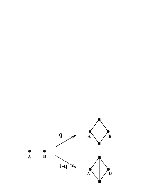
Figure 1: (Color online) Iterative construction method of the fractal networks. Each iterative link is replaced by a connected cluster on the right-hand side of the arrow. The red link is a noniterated link.

2.1 Construction algorithm

The proposed fractal networks have two categories of bonds (links or edges): iterative bonds and noniterated bonds which are depicted as solid and dashed lines, respectively. The networks are constructed in an iterative way as shown in Fig. 1. Let $F_{t}$ ($t\geq 0$) denote the networks after $t$ iterations. Then the networks are built in the following way: For $t=0$, $F_{0}$ is two nodes (vertices) connected by an iterative edge. For $t\geq 1$, $F_{t}$ is obtained from $F_{t-1}$. We replace each existing iterative bond in $F_{t-1}$ either by a connected cluster of links on the top middle of Fig. 1 with probability $q$, or by the connected cluster on the bottom right with complementary probability $1-q$. The growing process is repeated $t$ times, with the fractal graphs obtained in the limit $t\to\infty$. Figure 2 shows a network after three-generation growth for a specific case of $q=0.6$.

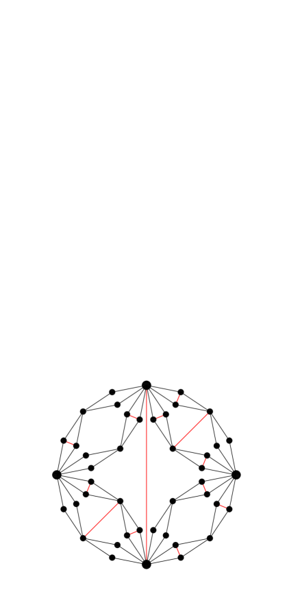
Figure 2: (Color online) Sketch of a network after three iterations for the particular case of $q=0.6$.

Next we compute the numbers of total nodes and edges in $F_{t}$. Let $L_{v}(t)$, $L_{i}(t)$ and $L_{n}(t)$ be the numbers of nodes, iterative edges, and noniterated edges created at step $t$, respectively. Note that each of the existing iterative edges yields two nodes and four new iterative edges; at the same time this original iterative edge itself is deleted, which means that $L_{i}(t)$ is also the total number of iterative edges at time $t$. Then we have $L_{v}(t)=2\,L_{i}(t-1)$ and $L_{i}(t)=4\,L_{i}(t-1)$ for all $t>0$. Considering the initial condition $L_{i}(0)=1$, one can obtain $L_{i}(t)=4^{t}$ and $L_{v}(t)=2\times 4^{t-1}$. Thus the number of total nodes $N_{t}$ present at step $t$ is

$$N_{t}=\sum_{t_{i}=0}^{t}L_{v}(t_{i})=\frac{2\times 4^{t}+4}{3}.$$ (1)

On the other hand, at each construction step, each of the existing iterative edges may yield one noniterated link with probability $1-q$, so the expected value of $L_{n}(t)$ is $(1-q)\,L_{i}(t-1)$ for $t\geq 1$, i.e., $L_{n}(t)=(1-q)\,4^{t-1}$. Therefore, the total number of edges $E_{t}$ present at step $t$ is

$$E_{t}=L_{i}(t)+\sum_{t_{i}=1}^{t}L_{n}(t_{i})=\frac{(4-q)\,4^{t}-(1-q)}{3}.$$ (2)

The average node degree after $t$ iterations is $\langle k\rangle_{t}=\frac{2\,E_{t}}{N_{t}}$, which approaches $4-q$ in the infinite $t$ limit.

2.2 Degree distribution

When a new node $u$ enters the system at step $t_{u}$ ($t_{u}\geq 1$), it has two iterative edges. At the same time, with probability $1-q$ one noniterated edge is created and linked to node $u$. Let $L_{i}(u,t)$ be the number of iterative links emanated from node $u$ at step $t$, then $L_{i}(u,t_{u})=2$. Notice that at any subsequent step each iterative edge of $u$ is broken and generates two new iterative edges linked to $u$. Thus $L_{i}(u,t)=2\,L_{i}(u,t-1)=2^{t-t_{u}+1}$.

We define $k_{u}(t)$ as the degree of node $u$ at time $t$, then we have

$$\left\{\begin{array}[]{lc}{k_{u}(t)=2^{t-t_{u}+1},}&\ \hbox{with probability}\ q,\\ {{k_{u}(t)=2^{t-t_{u}+1}+1},}&\ \hbox{with probability}\ 1-q,\end{array}\right.$$ (3)

where the last term 1 in the second formula represents the noniterated link connected to node $u$. For the initial two nodes created at step 0, neither of them has a noniterated link, both nodes have a degree of $2^{t}$.

Equation (3) indicates that the degree spectrum of the networks is not continuous. It follows that the cumulative degree distribution [27, 28] is given by $P_{\rm cum}(k)=\frac{N_{t,k}}{N_{t}}$, where $N_{t,k}$ is the number of nodes whose degree is not less than $k$. When $t$ is large enough, we find $P_{\rm cum}(k)\approx k^{-2}$. So the degree distribution follows a power-law form with the exponent $\gamma=3$, which is independent of $q$. The same degree exponent has been obtained in the famous Barabási-Albert (BA) model [8].

2.3 Clustering Coefficient

The clustering coefficient [29] of a node $u$ with degree $k_{u}$ is the probability that a pair of neighbors of $u$ are themselves connected, which is given by $C(k_{u})=2b_{u}/[k_{u}(k_{u}-1)]$, where $b_{u}$ is the number of existing connections between the $k_{u}$ neighbors of $u$. For our networks, the clustering coefficient $C(k)$ for a single node with degree $k$ can be evaluated exactly. Note that except for those nodes born at step $t$, all existing links among the neighbors of a given node are noniterated ones, whose number is ease to calculate. For the initial two nodes, the expected existing noniterated links among the neighbors is $(1-q)2^{t-1}$. For each of those nodes created at step $\phi$ $(0<\phi<t)$, there are average $(1-q)2^{t-\phi}$ noniterated links among its neighbors. Finally, for the nodes generated at step $t$, some of them have a degree of $3$, the number of links between the neighbors of each is $2$; the others have a degree of $2$, their clustering coefficient is zero. Thus, there is a one-to-one correspondence between the clustering coefficient $C(k)$ of the node and its degree $k$:

$$C(k)=\left\{\begin{array}[]{lc}{\displaystyle{(1-q)/(k-1)}}&\ \hbox{for}\ k=2^{m}(2\leq m\leq t),\\ {\displaystyle{(1-q)/k}}&\ \hbox{for}\ k=2^{m}+1(2\leq m\leq t),\\ {\displaystyle{0}}&\ \hbox{for}\ k=2,\\ {\displaystyle{2/k}}&\ \hbox{for}\ k=3.\end{array}\right.$$ (4)

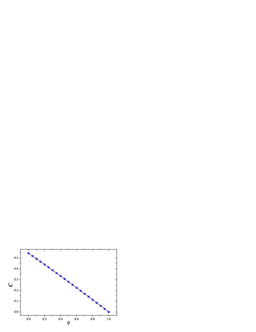
Figure 3: (Color online) The average clustering coefficient $C$ of the whole network as a function of $q$. It can be tunable systematically by changing $q$. The squares are the simulation results, and the line represents the analytical expression given by Eq. (5).

Using Eq. (4), we can obtain the clustering $\bar{C}_{t}$ of whole the network at step $t$, which is defined as the average clustering coefficient of all individual nodes. Then we have

$$\bar{C}_{t}= \frac{1-q}{N_{t}}\Bigg{[}\frac{L_{v}(0)}{2^{t}-1}+\sum_{r=1}^{t-1}\frac{qL_{v}(r)}{K_{r}-1}$$ (5)

$$+ \sum_{r=1}^{t-1}\frac{(1-q)L_{v}(r)}{K_{r}+1}+\frac{2\,L_{v}(t)}{K_{t}+1}\Bigg{]},$$

where $K_{r}=2^{t-r+1}$ and $K_{t}=2$. In the infinite network order limit ($N_{t}\rightarrow\infty$), $\bar{C}_{t}$ converges to a nonzero value $C$ as a function of parameter $q$. In the two extreme cases of $q=0$ and $q=1$, $C$ are 0 and 0.5435 [30], respectively. When $q$ increases from 0 to 1, $C$ grows from 0 to 0.5435, see Fig. 3. Thus, the parameter $q$ in our model introduces the clustering effect by allowing the formation of triangles. Furthermore, the relation between $C$ and $q$ is almost linear, as depicted in Fig. 3.

2.4 Average path length

Shortest paths play an important role both in the transport and communication within a network and in the characterization of the internal structure of the network [31, 32, 33, 34]. Let $d_{ij}$ represent the shortest path length from node $i$ to $j$, then the average path length (APL) $d_{t}$ of $F_{t}$ is defined as the mean of $d_{ij}$ over all couples of nodes in the network, and the maximum value $D_{t}$ of $d_{ij}$ is called the diameter of the network.

For general $q$, it is difficult to derive a closed formula for the APL $d_{t}$ of network $F_{t}$. But for two limiting cases of $q=0$ and $q=1$, both the networks are deterministic ones, we can obtain the analytic solutions for APL, denoted as $d_{t}^{0}$ and $d_{t}^{1}$, respectively. In the large $t$ limit, $d_{t}^{0}\approx\frac{8}{21}2^{t}$ [30] and $d_{t}^{1}\approx\frac{11}{21}2^{t}$ [23]. On the other hand, for large $t$ limit, $N_{t}\sim 4^{t}$, so both $d_{t}^{0}$ and $d_{t}^{1}$ grow as a square power of the number of network nodes.

By construction, it is obvious that $d_{t}^{0}$ and $d_{t}^{1}$ are the lower and upper bound of APL for network $F_{t}$, respectively. As a matter of fact, if we denote the specific $q=1$ case of the network as $F_{t}^{1}$ (it has no noniterated edges, and thus the maximum APL), then one can obtain $F_{t}$ from $F_{t}^{1}$ by adding noniterated edges in a certain way. The less the parameter $q$, the more the added noniterated edges. In the case of $q=0$, the network is the densest one with the minimum APL. Therefore, the APL is a decreasing function of $q$. As $q$ drops from 1 to 0, $d_{t}$ increases from $\frac{8}{21}2^{t}$ at $q=1$ to $\frac{11}{21}2^{t}$ at $q=0$. From above arguments, we can conclude that for the full range of $q$ between 0 and 1, the APL $d_{t}$ has an exponential growth with network size, which indicates that the considered networks $F_{t}$ are not small worlds.

2.5 Fractal dimension

To determine the fractal dimension, we follow the mathematical framework introduced in Ref. [16]. We are concerned about three quantities, network size $N_{t}$, network diameter $D_{t}$, and degree $k_{u}(t)$ of a given node $u$. By construction, we can easily see that in the infinite $t$ limit, these quantities grow obeying the following relation: $N_{t}\simeq 4\,N_{t-1}$, $D_{t}=2\,D_{t-1}$, $k_{u}(t)\simeq 2\,k_{u}(t-1)$. Thus, for large networks, $N_{t}$, $k_{u}(t)$ and $D_{t}$ increase by a factor of $f_{N}=4$, $f_{k}=2$ and $f_{D}=2$, respectively.

From above obtained microscopic parameters demonstrating the mechanism for network growth, we can derive the scaling exponents: the fractal dimension $d_{B}=\frac{\ln f_{N}}{\ln f_{D}}=2$ and the degree exponent of boxes $d_{k}=\frac{\ln f_{k}}{\ln f_{D}}=1$. According to the scaling relation of fractal scale-free networks, the exponent of the degree distribution satisfies $\gamma=1+\frac{d_{B}}{d_{k}}=3$, giving the same $\gamma$ as that obtained in the direct calculation of the degree distribution.

The fractality behavior can be also easy to see by tiling the system using a renormalization procedure as follows. we can ‘zoom out’ (i.e. renormalize) the network by replacing each connected cluster of bonds on the right of Fig. 1 by a single ‘super’-link, in a way that reverses the process of network growth, see Fig. 1. This has the effect of rescaling diameter, it reduces the diameter by a factor of $2$ by carrying a cluster of bonds with diameter 2 into a single ‘super’-link with unit length. At the same time, the number nodes of in the rescaled network decreases by a factor $=4$. Thus, the fractal dimension is $d_{B}=\frac{\ln 4}{\ln 2}=2$.

3 SIR model on the networks

As demonstrated in the preceding section, the networks exhibit simultaneously many interesting properties: scale-free phenomenon, tunable clustering, “large-world” behavior, and fractality. To the best of our knowledge, these features have not been reported in previous network models. Hence, it is of scientific interest and great significance to investigate dynamic processes taking place upon the model to inspect the effect of network topologies on the dynamics. Next we will focus on studying the SIR model of epidemics, which is one of the most important disease models and has attracted much attention within physical society, see [5] and references therein.

The standard SIR model [6, 7] assumes that each individual can be in any of three exclusive states: susceptible (S), infected (I), or removed (R). The dynamics of disease transmission on a network can be described as follows. Each node of the network stands for an individual and each link represents the connection along which the individuals interact and the epidemic can be transmitted. At each time step, an infected node transmits infection to each of its neighbors independently with probability $\lambda$; at the same time the infected node itself becomes removed with a constant probability 1, whereupon it can not catch the infection again, and thus will not infect its neighbors any longer.

The above-described SIR model for disease dynamics is equivalent to a bond percolation process with bond occupation probability equal to the infection rate $\lambda$ [35, 36]. The connected clusters of nodes in the bond percolation process then correspond to the groups of individuals that would be infected by a disease outbreak starting with any individual within the cluster it belongs to. It was shown that in scale-free networks such as Barabási-Albert (BA) network, for any vanishingly small $\lambda$, there exists an extensive spanning cluster or “giant component”, implying that scale-free networks demonstrate an absence of epidemic thresholds. However, we will present that for our networks, epidemic thresholds are present, the values of which depend on the parameter $q$.

According to the mapping between the SIR dynamics and the bond percolation problem, the epidemic threshold corresponds precisely to the percolation threshold. In our case, the recursive construction of the networks make it possible to study the percolation problem by using the real-space renormalization group technique [37, 38, 39] to obtain an exact solution for the percolation (epidemic) thresholds. Here we are interested in only the percolation phase transition point, excluding the size of giant cluster. Let us describe the procedure in application to the considered network. Supposing that the network growth stops at a time step $t\rightarrow\infty$, then we spoil the network in the following way: for an arbitrary present link in the undamaged network, it is retained in the damaged network with probability $\lambda$. Then we invert the transformation shown in Fig. 1 and define $n=t-\tau$ for this inverted transformation, which is in fact a decimation procedure [39]. Further, we introduce the probability $\lambda_{n}$ that if two nodes are connected in the undamaged network at $\tau=t-n$, then at the $n$th step of the decimation for the damaged network, there exists a path between these vertices. Here, $\lambda_{0}=\lambda$. According to the network construction and the analysis in [39], it is easy to obtain the following recursive relation for $\lambda_{n}$:

$$\lambda_{n+1}= q\left(\lambda_{n}^{2}+\lambda_{n}^{2}-\lambda_{n}^{2}\times\lambda_{n}^{2}\right)$$ (6)

$$+ (1-q)\Big{[}\lambda_{n}^{5}+5\lambda_{n}^{4}(1-\lambda_{n})$$

$$+ 8\lambda_{n}^{3}(1-\lambda_{n})^{2}+2\lambda_{n}^{2}(1-\lambda_{n})^{3}\Big{]}.$$

Equation (6) has five roots (i.e., fixed points), among which two are invalid: one is greater than 1, the other is less than 0. The other three fixed points are as follows: two stable fixed points at $\lambda=0$ and $\lambda=1$, and an unstable fixed point at $\lambda_{c}$ that is the percolation threshold. We omit the expression of $\lambda_{c}$ as a function of $q$, because it is very lengthy. We show the dependence of $\lambda_{c}$ on $q$ in Fig. 4, which indicates that the threshold $\lambda_{c}$ increases almost linearly as $q$ increases. When $q$ grows from 0 to 1, $\lambda_{c}$ increases from 0.5 to $\frac{\sqrt{5}-1}{2}\approx 0.618$.

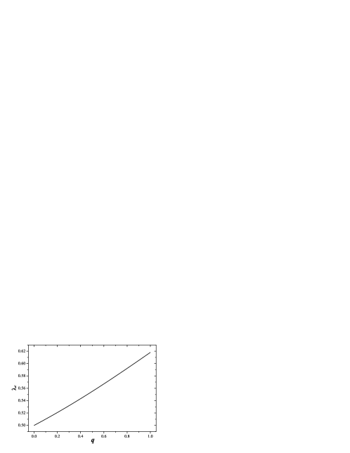
Figure 4: The dependence relation of percolation threshold $\lambda_{c}$ on the parameter $q$.

Therefore, there exists a percolation threshold $\lambda_{c}$ such that for $\lambda>\lambda_{c}$ a giant component appears, for $\lambda<\lambda_{c}$ there are only small clusters. This means that for the SIR model the epidemic prevalence undergoes a phase transition at a nonzero epidemic threshold $\lambda_{c}$. If the infection rate $\lambda>\lambda_{c}$, the disease spreads and becomes persistent in time; otherwise, the infection dies out gradually. The existence of epidemic thresholds in our networks is in sharp contrast with the null threshold found in a wide range of stochastic scale-free networks of the Barabási-Albert (BA) type [9, 10, 11].

Why are the present scale-free networks not prone to disease propagation as previously studied uncorrelated BA type scale-free networks? We argue that the presence of finite epidemic thresholds in our networks lies with their two-dimensional fractal structure with diameter increasing as a square power of network order, a property analogous to that of two-dimensional regular lattice [40]. The ‘large-world’ feature stops the diffusion of diseases, and makes the behaviors of disease spreading in our networks similar to those of regular lattices. Thus, the fractal topology provides protection against disease spreading.

4 Conclusions

In the present work, we have introduced a new model for fractal networks and provided a detailed analysis of the structural properties, which are related to the model parameter $q$. The model exhibits a rich topological behavior. The degree distribution is power-law with the degree exponent asymptotically approaching 3 for large network order. The clustering coefficient is changeable, which can be systematically tunable in a large range by altering $q$. Particularly, the networks are topologically fractal with a fractal dimension of 2 for all $q$. Along with the fractality, the networks display ‘large-world’ phenomenon, their average path length increases approximatively as a square power of the number of nodes.

We have also investigated the effects of the particular topological characteristics on the SIR model for disease spreading dynamics. Strikingly, We found that epidemic thresholds are recovered for all networks regardless the value of $q$, which is in contrast to the conventional wisdom that being prone to disease propagation is an intrinsic nature of scale-free networks. We concluded that the dominant factor suppressing epidemic spreading is the fractal structure accompanied by a ‘large-world’ behavior. The peculiar structural properties and epidemic dynamics make our networks unique within the category of scale-free networks. Our study is helpful for designing real-life networked systems robust to epidemic outbreaks, and for better understanding of the effluences of structure on the propagation dynamics.

References

- [1] R. Albert and A.-L. Barabási, Rev. Mod. Phys. 74, 47 (2002).
- [2] S.N. Dorogovtsev and J.F.F. Mendes, Adv. Phys. 51, 1079 (2002).
- [3] M.E.J. Newman, SIAM Rev. 45, 167 (2003).
- [4] S. Boccaletti, V. Latora, Y. Moreno, M. Chavez and D.-U. Hwanga, Phys. Rep. 424, 175 (2006).
- [5] M. Barthélemy, A. Barrat, R. Pastor-Satorras, and A. Vespignani, J. Theor. Biol. 235, 275 (2005).
- [6] N. T. Bailey, The Mathematical Theory of Infectious Diseases (Macmillan, New York, 1975), 2nd ed.
- [7] H. W. Hethcote, SIAM Rev. 42, 599 (2000).
- [8] A.-L. Barabási and R. Albert, Science 286, 509 (1999).
- [9] R. Pastor-Satorras and A. Vespignani, Phys. Rev. Lett. 86, 3200 (2001).
- [10] R. Pastor-Satorras and A. Vespignani, Phys. Rev. E 63, 066117 (2001).
- [11] Y. Moreno, R. Pastor-Satorrasand, and A. Vespignani, Eur. Phys. J. B 26, 521 (2002).
- [12] M. Serrano and M. Boguñá, Phys. Rev. Lett. 97, 088701 (2006).
- [13] M. Boguñá, R. Pastor-Satorras, and A. Vespignani, Phys. Rev. Lett. 90, 028701 (2003).
- [14] L. da. F. Costa, F.A. Rodrigues, G. Travieso, and P.R.V. Boas, Adv. Phys. 56, 167 (2007).
- [15] C. Song, S. Havlin, H. A. Makse, Nature 433, 392 (2005).
- [16] C. Song, S. Havlin, H. A. Makse, Nature Phys. 2, 275 (2006).
- [17] C. Song, L. K. Gallos, S. Havlin, H. A. Makse, J. Stat. Mech.:Theory Exp. P03006, (2007).
- [18] J. S, Kim, K.-I. Goh, B. Kahng, and D Kim, Chaos 17, 026116 (2007).
- [19] M. Kitsak, S. Havlin, G. Paul, M. Riccaboni, F. Pammolli, and H. E. Stanley, Phys. Rev. E 75, 056115 (2007).
- [20] S.-H. Yook, F, Radicchi, and H. M.-Ortmanns, Phys. Rev. E 72, 045105(R) (2006).
- [21] Z. Z. Zhang, S. G. Zhou, and T. Zou, Eur. Phys. J. B 56, 259 (2007).
- [22] M. Hinczewski, Phys. Rev. E 75, 061104 (2007).
- [23] M. Hinczewski and A. N. Berker, Phys. Rev. E 73, 066126 (2006).
- [24] L. K. Gallos, C. Song, S. Havlin, H. A. Makse, Proc. Natl Acad. Sci. USA 10, 7746 (2007).
- [25] S. Condamin, O. Bénichou, V. Tejedor, R. Voituriez, and J. Klafter, Nature 450, 77 (2007).
- [26] H. D. Rozenfeld, S. Havlin, and D. ben-Avraham, New J. Phys. 9, 175 (2007).
- [27] S. N. Dorogovtsev, A. V. Goltsev, and J. F. F. Mendes, Phys. Rev. E 65, 066122 (2002).
- [28] Z. Z. Zhang, S. G. Zhou, T. Zou, L. C. Chen, and J. H. Guan, Eur. Phys. J. B 60, 259 (2007).
- [29] D.J. Watts and H. Strogatz, Nature (London) 393, 440 (1998).
- [30] Z. Z. Zhang, S. G. Zhou, T. Zou, and J. H. Guan, (unpublished).
- [31] A. Fronczak, P. Fronczak, and J. A. Hołyst, Phys. Rev. E 70, 056110 (2004).
- [32] J. A. Hołyst, J. Sienkiewicz, A. Fronczak, P. Fronczak, and K. Suchecki, Phys. Rev. E 72, 026108 (2005).
- [33] S. N. Dorogovtsev, J. F. F. Mendes, and J. G. Oliveira, Phys. Rev. E 73, 056122 (2006).
- [34] Z.Z. Zhang, L.C. Chen, S.G. Zhou, L.J. Fang, J.H. Guan, and T. Zou, Phys. Rev. E 77, 017102 (2008).
- [35] P. Grassberger, Math. Biosci. 63, 157 (1982).
- [36] M. E. J. Newman, Phys. Rev. E 66, 016128 (2002).
- [37] A.A. Migdal, Zh. Eksp. Teor. Fiz. 69, 1457 (1975) [Sov. Phys. JETP 42, 743 (1976)].
- [38] L.P. Kadanoff, Ann. Phys. (N.Y.) 100, 359 (1976).
- [39] S. N. Dorogovtsev, Phys. Rev. E 67, 045102(R) (2003).
- [40] M. E. J. Newman, J. Stat. Phys. 101 819 (2000).