Generation of quantum-dot cluster states with superconducting transmission line resonator

Abstract

We propose an efficient method to generate cluster states in spatially separated double quantum dots with a superconducting transmission line resonator (TLR). When the detuning between the double-dot qubits transition frequency and the frequency of the full wave mode in the TLR satisfies some conditions, an Ising-like operator between arbitrary two separated qubits can be achieved. Even including the main noise sources, it’s shown that the high fidelity cluster states could be generated in this solid system in just one step.

Introduction.— Quantum entanglement is the root in quantum computation J. Gruska , quantum teleportation Bennett , quantum dense coding Bennett2 , and quantum cryptography Artur . However, it’s challenging to create multi-particle entangled states in experiment. In 2001 Briegel and Raussendorf introduced a highly entangled states, the cluster states Hans J. Briegel , which can be used to perform universal one way quantum computation. Up to now, various schemes are proposed to generate cluster states in many different types of physical systems. Especially, it has been argued that the cluster states can be generated effectively in solid state system, such as superconductor charge qubit Tetsufumi Tanamoto ; J.Q. You ; Zheng-Yuan Xue and semiconductor quantum dot Massoud ; Hui Zhang ; Yaakov .

Electron spins in semiconductor quantum dots are one of the most promising candidates for a quantum bit, due to their potential of long coherence time Taylor ; Golovach ; Khaetskii . Producing cluster states in quantum dots, has been discussed within Heisenberg interaction model Massoud and Ising-like interaction model Hui Zhang , where the long-term interaction inversely ratios to the distance between non-neighboring qubits. Recently Childress and Taylor et al. introduced a technique to electrically couple electron charge states or spin states associated with semiconductor double quantum dots to a TLR via capacitor Taylor2 ; Childress . The qubit is encoded on the quantum double-dot triplet and singlet states. The interaction Hamiltonian between the qubits and the TLR is a standard Jaynes-Cumming (JC) model Hui Zhang2 . A switchable long-range interaction can be achieved between any two spatially separated qubits with the TLR cavity field. This technique open a new avenue for quantum information implementation.

In this work, we find when the detuning between the qubits transition frequency and the frequency of the full wave mode in the TLR satisfies some conditions, an Ising-like operator between arbitrary two separated qubits can be achieved from the JC interaction. The highly entangled cluster states can be generated one step with the auxiliary of an oscillating electric field. Finally, we discuss the feasibility and the cluster states fidelity of our scheme.

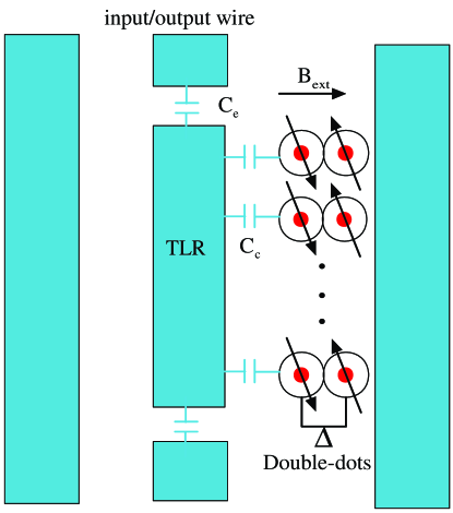
Figure 1: (Color online) Schematic diagram of a TLR and several double quantum dots coupled system. A detailed circuit representation of the TLR cavity (blue) can be found in Fig.1 of Ref.Blais . The double dots are biased with an external potential $\Delta$, and capacitive coupling $C_{c}$ with the TLR. The TLR is connected to the input/output wiring with a capacitor $C_{e}$.

Preparation of cluster states.— The system we study includes N identical double-dot qubits capacitively coupling with a TLR by $C_{c}$, as shown in Fig. (1). The TLR is coupled to input/output wiring with a capacitor $C_{e}$ to transmit signals. Two electrons are localized in double-dot quantum molecule. The two electrons charge states, spin states and the corresponding eigenenergies are controlled by several electrostatic gates.

An external magnetic field is applied along axis $z$. At a large static magnetic field ($100$ mT), the spin aligned states ($\left|\left(1,1\right)T_{+}\right\rangle=\left|\uparrow\uparrow\right\rangle$, $\left|\left(1,1\right)T_{-}\right\rangle=\left|\downarrow\downarrow\right\rangle$) are splitted from spin anti-aligned states ($\left|\left(1,1\right)T_{0}\right\rangle=\left(\left|\uparrow\downarrow\right\rangle+\left|\downarrow\uparrow\right\rangle\right)/\sqrt{2}$ , $\left|\left(1,1\right)S\right\rangle=\left(\left|\uparrow\downarrow\right\rangle-\left|\downarrow\uparrow\right\rangle\right)/\sqrt{2}$) due to Zeeman splitting. The notation ($n_{l},n_{r}$) indicates $n_{l}$ electrons on the ”left” dot and $n_{r}$ electrons on the ”right” dot. In addition to the $(1,1)$ subspace, the doubly-occupied state $\left|(0,2)S\right\rangle$ is coupled to $\left|(1,1)S\right\rangle$ via tunneling $T_{c}$. $\left|(0,2)S\right\rangle$ and $\left|(1,1)S\right\rangle$ have a potential energy difference of $\Delta$. Due to the tunneling between the two adjacent dots, the $\left|(1,1)S\right\rangle$ and $\left|(0,2)S\right\rangle$ hybridize. We can get the double dots eigenstates:

$$\left|+\right\rangle = -\sin{\theta}\left|\left(1,1\right)S\right\rangle+\cos{\theta}\left|\left(0,2\right)S\right\rangle,$$ (1)

$$\left|-\right\rangle = \cos{\theta}\left|\left(1,1\right)S\right\rangle+\sin{\theta}\left|\left(0,2\right)S\right\rangle,$$ (2)

where $\tan{\theta}=-2T_{c}/(\Omega+\Delta)$ and $\Omega=\sqrt{4T_{c}^{2}+\Delta^{2}}$. $\Omega$ is the energy gap between the eigenstates $\left|+\right\rangle$ and $\left|-\right\rangle$. We can choose $\Delta=0$ in order to suppress the fluctuations in control electronics, then $\left|+\right\rangle=(\left|\left(1,1\right)S\right\rangle+\left|(0,2)S\right\rangle)/\sqrt{2}$, $\left|-\right\rangle=(\left|\left(1,1\right)S\right\rangle-\left|(0,2)S\right\rangle)/\sqrt{2}$. The qubit is encoded on the states $|+\rangle$ and $|-\rangle$.

An oscillating electric field, which frequency is coincidental with the qubit energy gap, is applied to the left side gate of the double quantum dots. The single-qubit operation Hamiltonian in the interaction picture can be expressed as

$$H_{i}=\eta\left|(1,1)S\right\rangle\left\langle(1,1)S\right|=\eta(I+\sigma_{i}^{x})=\eta\sigma_{i}^{x},$$ (3)

where $\eta=\hat{d}\cdot\hat{E}$, $\hat{d}$ is the dipole of left quantum dot and $\hat{E}$ is the oscillating electric field.

We consider a TLR of length L, with capacitance per unit length $C_{0}$, and characteristic impedance $Z_{0}$. Neglecting the higher energy modes, we can only consider the full wave mode, with the wavevector $k=\frac{\pi}{L}$, and frequency $\omega=\frac{k}{C_{0}Z_{0}}$ Childress . The TLR can be described by the Hamiltonian $H_{\mathrm{cavity}}=\omega a^{\dagger}a$, where $\hbar=1$, $a^{\dagger}$, $a$ are the creation and annihilation operators for the full wave mode of the TLR. In the interaction picture, the interaction between N qubits and the TLR can be described by the Hamiltonian Hui Zhang2

$$H_{\mathrm{int}}=g_{0}\sum_{i=1}^{N}(e^{i\delta t}a^{\dagger}\sigma_{i}^{-}+e^{-i\delta t}a\sigma_{i}^{+}),$$ (4)

where $\sigma_{i}^{+}=\left|+\right\rangle\left\langle-\right|$, $\sigma_{i}^{-}=\left|-\right\rangle\left\langle+\right|$, $\sigma_{i}^{x}=\sigma_{i}^{+}+\sigma_{i}^{-}$, $\delta=\omega-\Omega$. Here we can presently assume the coupling strength is homogenous. The overall coupling coefficient can be described by Childress

$$g_{0}=\omega\frac{C_{c}}{2C_{tot}}\sqrt{\frac{2z_{0}}{R_{Q}}},$$ (5)

where $R_{Q}=h/e^{2}\approx 26$ k$\Omega$. $C_{tot}$ is the total capacitance of the double-dot.

If the interaction time $\tau$ satisfies

$$\delta\tau=2k\pi,$$ (6)

the evolution operator for the interaction Hamiltonian (4) can be expressed as Zheng

$$U(\tau)=exp(-i\frac{\lambda}{2}\tau(\sum_{i=1}^{N}{{\sigma_{i}^{x}}})^{2})=exp(-i\lambda\tau\sum_{j>i=1}^{N}\sigma_{i}^{x}\sigma_{j}^{x}),$$ (7)

where $\lambda=g_{0}^{2}/2\delta$.

When $\Delta$ is changed to zero, the coupling coefficient between the qubits and TLR is maximal. An oscillating electric field is applied to all the qubits at the same time. In the interaction picture, the total Hamiltonian of the system can be written as

$$H_{tot}=g_{0}\sum_{i=1}^{N}(e^{i\delta t}a^{\dagger}\sigma_{i}^{-}+e^{-i\delta t}a\sigma_{i}^{+})+\eta\sum_{i=1}^{N}\sigma_{i}^{x}.$$ (8)

When the operation time $\tau$ satisfies the condition (6), we can obtain the total evolution operator

$$U(\tau)=exp(-i\eta\tau\sum_{i=1}^{N}{\sigma_{i}^{x}}-i\lambda\tau\sum_{j>i=1}^{N}\sigma_{i}^{x}\sigma_{j}^{x}).$$ (9)

When $\eta=(N-1)\lambda$, the total evolution operator is given by

$$U(\tau)=exp(-4i\lambda\tau\sum_{j>i=1}^{N}\frac{1+\sigma_{i}^{x}}{2}\frac{1+\sigma_{j}^{x}}{2}).$$ (10)

In order to generate the cluster states, the initial state of N qubits should be prepared in the state $\bigotimes_{i=1}^{N}\left|-\right\rangle_{i}=\frac{1}{\sqrt{2}}\bigotimes_{i=1}^{N}(\left|0\right\rangle_{i}+\left|1\right\rangle_{i})$, where $\left|0(1)\right\rangle_{i}=\frac{1}{\sqrt{2}}(\left|-\right\rangle_{i}\pm\left|+\right\rangle_{i})$ are the eigenstates of $\sigma_{i}^{x}$ with the eigenvalues $\pm 1$. Next we would discuss how to prepare the initial state in experiment. Firstly we can prepare the two electrons in double quantum dots to the state $|(0,2)S\rangle$ at a large positive potential energy difference $\Delta$ Petta . Then the $|(0,2)S\rangle$ can be changed to the state $|-\rangle=(|(1,1)S\rangle-|(0,2)S\rangle)/\sqrt{2}$ by rapid adiabatic passage Taylor . After the initial state has been prepared, the qubits would be resonantly coupled with the TLR. We apply an oscillating electric field to each qubits at the same time. Thus the initial state would evolve under the total operator (10). If the evaluation interaction time satisfies

$$4\lambda\tau=(2n+1)\pi,$$ (11)

with $n$ being integer, the spatially separated double quantum dots can be generated to the cluster states

$$\left|\Psi\right\rangle_{N}=\frac{1}{2^{N/2}}\bigotimes_{i=1}^{N}(\left|0\right\rangle_{i}(-1)^{N-i}\prod_{j=i+1}^{N}\sigma_{i}^{x}+\left|1\right\rangle_{i}).$$ (12)

The effective coupling coefficient $g_{0}\frac{2T_{c}}{\Omega}$ can be tuned by external potential $\Delta$. When $\Delta$ is changed, the states $|0(1)\rangle$ would change according to Eq. (1), (2), but the expression (12) of the cluster states is unchanged. When the cluster states is generated at the time of $\tau$, we can remove the oscillating electric field and change $\Delta$ to discouple all the qubits to the TLR. Then the cluster states can be preserved.

Feasibility of the scheme.— The sample of the TLR and quantum dots coupled system can be obtained in a two-step fabrication process on a GaAs/AlGaAs heterostructure. Firstly, quantum dots are formed in the two-dimensional electron gas below the surface, using electron beam lithography and Cr-Au metallization. Then the TLR is fabricated by conventional optical lithography Wallraff . The main technical challenges for experimental implementation of our proposal are the design and nanofabrication of the sample Schusterthesis . The diameter of the quantum dot is about $400$ nm, and the corresponding capacitance of the double-dot $C_{tot}$ is about $200$ aF. The distance between the two double-dot molecules should be $4$ $\mu$m which is tenfold of the distance between two quantum dots within a double-dot. Thus we can neglect the interaction between the double-dot molecules safely Guo . Since the energy gap between $\left|+\right\rangle$ and $\left|-\right\rangle$ is about $10$ $\mu$eV at the operation point, the experimental manipulation should be implemented in dilution refrigerator with temperature below $100$ mK. Both the conditions (6) and (11) are satisfied whenever $\delta=g_{0}\sqrt{4k/(2n+1)}$. From Eq. (5) the coupling coefficient $g_{0}$ can be up to $\omega/16$ with a large coupling capacitor $C_{c}\approx 2C_{tot}\approx 400$ aF. For $k=1$, $n=0$, $\omega/2\pi=2$ GHz and $g_{0}/2\pi=125$ MHz, the operation time of the generation of cluster states is $\tau=\frac{2\pi}{\delta}=4$ ns.

Decoherence.— In our system, the main decoherence processes are the dissipation of the TLR, the spin dephasing, charge relaxation and additional dephasing of the double-dot molecules. The dissipation of the TLR occurred through coupling to the external leads can be described by the photon decay rate $\kappa=\omega/Q$, where $Q$ is the quality factor. For $Q=1\times 10^{5}$, $\omega=2\pi\times 2$ GHz in our situation, the photon decay time $1/\kappa\approx 50$ $\mu$s is $4$ orders longer than the operation time $\tau$. Therefore the cavity loss can be neglected in our situation.

Nuclear spins are one of the main noise sources in semiconductor quantum dots via hyperfine interaction. The hyperfine field can be treated as a static quantity, because the evolution of the random hyperfine field is several orders slower ($>10$ $\mu$s) than the electron spin dephasing. In the operating point, the most important decoherence due to hyperfine field is the spin dephasing between the states $|(1,1)S\rangle$ and $|(1,1)T_{0}\rangle$. By suppressing nuclear spin fluctuations Marcus2008 , the spin dephasing time obtained by quasi-static approximation can be $T^{*}_{2}=\hbar/(g\mu_{B}\langle\Delta B_{n}^{z}\rangle_{rms})\approx 1$ $\mu$s, where $\Delta B_{n}^{z}$ is the nuclear hyperfine gradient field between two dots and rms denotes a root-mean-square time-ensemble average. The coupling to the phonon bath will lead to the relaxation of the charge freedom. Using the spin-boson model, the relaxation time of the qubits can be obtained by Fermi-Golden rule Taylor2 . The charge relaxation time $T_{1}$ is about $1$ $\mu$s at the operation point. Additional dephasing is assumed to arise from the low frequency fluctuations of the control electronics, which typically have the $1/f$ spectrum. In our system, it’s assumed that the origin of $1/f$ noise is the random drift of the gate bias when an electron tunnel in or out of the metallic electrode. Assuming $1/f$ noise subject to Gaussian statistics, we found the addition dephasing time $T_{2,\alpha}\sim\Omega T_{2,bare}^{2}$ is about $100$ ns at the optimal working point ($\Delta\approx 0$), where $T_{2,bare}$ will be discussed below in detail and can be up to $10$ ns. Thus the total operation time of the present proposal $\tau\approx 4$ ns is much shorter than the spin dephasing time, charge relaxation and additional dephasing time of the qubits.

Fidelity of the cluster states.— For simplicity, we assume the control electronics fluctuations are Gaussian. These noises would lead to the fluctuations of the parameter $\lambda$ via the electric potential difference $\Delta$. Suppose $\Delta_{i}(t)=\Delta+\epsilon_{i}(t)$, $\left\langle\epsilon_{i}(t)\right\rangle=0$, $\left\langle\epsilon_{i}(t)\epsilon_{j}(t{{}^{\prime}})\right\rangle=\int S_{ij}(\omega)e^{i\omega(t-t^{\prime})}d\omega$ ($i$ labeling the $i$-th qubit). The fluctuations of the oscillating electric field would result in the fluctuations of the parameter $\eta$. The fluctuations of $\lambda$ and $\eta$ would add an unwanted phase $\theta_{i}$ to the desired value $\pi$ TAME . Including the fluctuations, the evolution operator (10) should be rewritten in the form of

$$U(\tau)=exp(-i\pi\sum_{j>i=1}^{N}\frac{1+\sigma_{i}^{x}}{2}\frac{1+\sigma_{j}^{x}}{2})exp(-i\int_{0}^{\tau}\delta\eta(t)dt\sum_{i=1}^{N}{\sigma_{i}^{x}})exp(-i\int_{0}^{\tau}\delta\lambda(t)dt\sum_{j>i=1}^{N}{\sigma_{i}^{x}\sigma_{j}^{x}}),$$ (13)

where $\lambda(t)=\lambda+\delta\lambda(t)$ and $\eta(t)=\eta+\delta\eta(t)$. Since $\delta\lambda+\frac{\delta\eta}{N-1}$, $\delta\eta+(N-1)\delta\lambda$ are larger than $\delta\lambda$, $\delta\eta$, we can write the unwanted phase $\theta_{i}=\int_{0}^{\tau}{4(\delta\lambda(t)+\frac{\delta\eta(t)}{N-1})dt}=\theta_{1,i}+\theta_{2,i}$, where $\theta_{1,i}=\int_{0}^{\tau}{4\delta\lambda(t)}dt$ and $\theta_{2,i}=\int_{0}^{\tau}{4\frac{\delta\eta(t)}{N-1}}dt$.

Since $\delta$, $\lambda$ satisfy Gaussian distribution, $\theta_{1,i}$, $\theta_{2,i}$, $\theta_{i}$ have Gaussian distribution $G(0,\sigma_{1,i}^{2})$, $G(0,\sigma_{2,i}^{2})$, $G(0,\sigma_{i}^{2})$. Ignoring the correlative fluctuations, the variance of $\theta_{1,i}$ at the optimal working point is

$$\sigma_{1,i}^{2}=(\frac{2g_{0}^{2}}{\Omega\delta^{2}})^{2}\left\langle(\int_{0}^{\tau}\epsilon^{2}(t)dt)^{2}\right\rangle,$$ (14)

where

$$\begin{array}[]{llll}\left\langle(\int_{0}^{\tau}{\ \epsilon^{2}(t)dt})^{2}\right\rangle&=&(\int S_{i}(\omega)d\omega)^{2}\tau^{2}&\\ &&+2(\int S_{i}(\omega)\frac{\sin\omega\tau}{\omega\tau}d\omega)^{2}\tau^{2}.&\end{array}$$ (15)

For the low frequency noise, $S_{i}(\omega)$ has a high frequency cutoff $\gamma\ll\frac{1}{\tau}$. Therefore we can get $\left\langle(\int_{0}^{\tau}{\epsilon^{2}(t)dt})^{2}\right\rangle=3(\int S_{i}(\omega)d\omega)^{2}\tau^{2}$. Assuming $\frac{1}{T_{2,bare}^{2}}=\int S_{i}(\omega)d\omega$, we can obtain the variance $\sigma_{1,i}^{2}=\frac{12g_{0}^{4}}{\delta^{4}}(\frac{\tau}{\Omega T_{2,bare}^{2}})^{2}$. Taking $T_{2,bare}\approx 10$ ns from the Ref. Petta ; Bracher ; Koppens , the variance of $\theta_{1,i}$ is $\sigma_{1,i}=0.022\pi$. The fluctuations of the oscillating electric field root in the electronics noise. The fluctuations can be reduced in a small value with better high- and low-frequency filtering technique. Supposing $\sigma_{\Delta\eta}/\Delta\eta\approx 2\%$, the variance of $\theta_{2,i}$ is $\sigma_{2,i}=0.006\pi$. So $\theta_{i}$ has an Gaussian distribution $G(0,(0.023\pi)^{2})$. The fidelity of N qubits cluster states is calculated according to the formula $F=|2^{-N}\sum_{z_{i}}\prod_{j=1}^{N-1}(\int\frac{1}{\sqrt{2\pi}\sigma_{i}}e^{-\frac{\theta_{j}^{2}}{2\sigma_{i}^{2}}}e^{i\theta_{j}}d\theta_{j})^{z_{j}z_{j+1}}|^{2}$ from Ref. TAME , as shown in Fig. (2). The fidelity of a 30-qubit cluster states can be $96.2\%$.

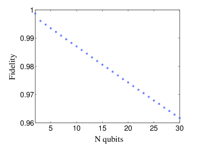
Figure 2: The fidelity of N-qubit cluster states.

Conclusion and Discussions.— Distinguished from cavity quantum electrodynamics in atomic quantum information processing, our scheme can realize the long-range interaction among the double-dot molecules with the TLR in a solid micro-chip device. This technique can couple the static qubit in the solid state system to the flying qubit (the cavity photon) Taylor2 . Compared with other schemes, the present proposal based on quantum dot molecules has four potential advantages: integration and scaling in a chip, easy-addressing, high controllability, and long coherence time associated with the electron spin. As discussed above, the preparation of the initial state can be easily implemented without inter-qubit coupling in our scheme. When the initial state has been prepared, the quantum-dot cluster states can be produced with only one step. The cluster states can be preserved easily by switching off the coupling between the qubits and TLR cavity field.

In conclusion, we proposed a realizable scheme to generate cluster states only one step in a new scalable solid state system, where the spatially separated semiconductor double-dot molecules are capacitive coupling with a TLR. An effective, switchable long-range interaction can be achieved between any two double-dot qubits with the assistance of TLR cavity field. The experimental related parameters and the possible fidelity of generated cluster states have been analyzed. Due to the long relaxation and dephasing time at the optimal working point, the present scheme seems implementable within today techniques.

This work was funded by National Basic Research Programme of China (Grants No. 2009CB929600, No. 2006CB921900), the Innovation funds from Chinese Academy of Sciences, and National Natural Science Foundation of China (Grants No. 10604052, No.10804104, No. 10874163).

References

- (1) J. Gruska, Quantum Computing (London: McGraw-Hill, New York, 1999).
- (2) C. H. Bennett et al., Phys. Rev. Lett. 70, 1895 (1993).
- (3) C. H. Bennett, S. J. Wiesner, Phys. Rev. Lett. 69, 2881 (1992).
- (4) A. K. Ekert, Phys. Rev. Lett. 67, 661 (1991).
- (5) H. J. Briegel and R. Raussendorf, Phys. Rev. Lett. 86, 910 (2001).
- (6) T. Tanamoto, Y. X. Liu, S. Fujita, X. Hu and F. Nori, Phys. Rev. Lett. 97, 230501 (2006).
- (7) J. Q. You, X. B. Wang, T. Tanamoto and F. Nori, Phys. Rev. A. 75, 052319 (2007).
- (8) Z. Y. Xue and Z. D. Wang, Phys. Rev. A. 75, 064303 (2007).
- (9) M. Borhani and D. Loss, Phys. Rev. A. 71, 034308 (2005).
- (10) G. P. Guo, H. Zhang, T. Tu and G. C. Guo, Phys. Rev. A. 75, 050301(R) (2007).
- (11) Y. S. Weinstein, C. S. Hellberg, and J. Levy, Phys. Rev. A. 72, 020304(R) (2005).
- (12) J. M. Taylor et al., Phys. Rev. B 76, 035315 (2007).
- (13) V. N. Golovach, A. Khaetskii, and D. Loss, Phys. Rev. Lett. 93, 016601 (2004).
- (14) A. V. Khaetskii and Y. V. Nazarov, Phys. Rev. B 61, 12639 (2000).
- (15) J. M. Taylor and M. D. Lukin, arXiv: cond-mat/0605144.
- (16) L. Childress, A. S. Sørensen, and M. D. Lukin, Phys. Rev. A 69, 042302 (2004).
- (17) G. P. Guo, H. Zhang, Y. Hu, T. Tu, and G. C. Guo, Phys. Rev. A 78, 020302(R) (2008).
- (18) A. Blais et al., Phys. Rev. A.75, 032329 (2007).
- (19) S. B. Zheng, Phys. Rev. A. 66, 060303(R) (2002).
- (20) J. R. Petta et al., Science 309, 2180 (2005).
- (21) A. Wallraff et al., Nature 431, 162 (2004).
- (22) D. I. Schuster, PhD Thesis, Yale University (2007).
- (23) G. P. Guo et al. Eur.Phys. J. B 61, 141 (2008).
- (24) A. S. Bracker et al., Phys. Rev. Lett. 94, 047402 (2005).
- (25) F. H. L. Koppens et al., Science 309, 1346 (2005).
- (26) D. J. Reilly et al., Science 321, 817 (2008).
- (27) M. S. Tame, M. Paternostro, M. S. Kim and V. Vedral, Int. J. Quantum Inf. 4, 689 (2006).