Density Functional Theory of Inhomogeneous Liquids: II. A Fundamental Measure Approach

Abstract

Previously, it has been shown that the direct correlation function for a Lennard-Jones fluid could be modeled by a sum of that for hard-spheres , a mean-field tail and a simple linear correction in the core region constructed so as to reproduce the (known) bulk equation of state of the fluid(Lutsko, JCP 127, 054701 (2007)). Here, this model is combined with ideas from Fundamental Measure Theory to construct a density functional theory for the free energy. The theory is shown to accurately describe a range of inhomogeneous conditions including the liquid-vapor interface, the fluid in contact with a hard wall and a fluid confined in a slit pore. The theory gives quantitatively accurate predictions for the surface tension, including its dependence on the potential cutoff. It also obeys two important exact conditions: that relating the direct correlation function to the functional derivative of the free energy with respect to density, and the wall theorem.

I Introduction

The insights of Van der Waals (VDW)Rowlinson (1979); van der Waals (1894) still underlie much of the work on nonuniform fluids. One such insight is that the free energy of a fluid can be separated into two contributions: the first due to the short-ranged repulsion of all interaction models, the second due to a long-ranged attraction. The former is generally treated using an effect hard-sphere contribution and the latter by a mean-field approximation. This model is attractive because of its simplicity and the prospect that it can be extended to complex systems such as molecular fluids, anisotropic interactions etc. However, while it can generally give reasonable qualitative predictions, such a simple model is seldom quantitatively accurate. It would therefore be highly desirable to modify the basic VDW model so as to give quantitatively accurate predictions if this can be done without compromising the basic simplicity of the model. The goal of this paper is to describe such a model and to show by application to the liquid-vapor interface and to fluids in confined geometries that it does indeed satisfy the twin requirements of accuracy and simplicity.

In the language of density functional theory, the VDW model can be described as a particular approximation to the direct correlation function (DCF) of the bulk fluid: namely that it is the combination of a hard-sphere DCF and a mean-field tail. In a previous paperLutsko (2007) it was noted that the failure of this model for the DCF lies primarily within the core region and that a good first order correction could be obtained by adding to the hard-sphere DCF a simple linear correction with coefficients adjusted to give continuity of the DCF and to give the correct thermodynamics. (The bulk thermodynamics are assumed to be known from e.g. thermodynamic perturbation theory or liquid state theory.) This is a satisfying approach as one of the motivations behind DFT (particularly the effective-liquid approaches) has been the idea that the DCF is a relatively simple function which could be easily approximated, in contrast to, say, the pair-distribution function which is highly structured. However, having a model DCF for the bulk fluid is only a first step towards describing non-uniform fluids: this model must somehow be used to construct a free-energy functional for nonuniform systems. If the DCF for an arbitrary nonuniform system were known, the free energy could be obtained immediately since the DCF is the second functional derivative of the free energy with respect to density. Thus one approach is to guess a generalization of the known DCF for a uniform system. In fact, since such functionals are known for the hard-sphere system and since the mean-field tail is independent of density, the generalization need only be guessed for the core-correction which limits the problem. In ref. Lutsko (2007), the usual ideas from DFT, involving the introduction of local densities into bulk expressions, were used to construct such a functional with mixed success: while the model gave reasonable predictions for the surface tension of the liquid-vapor interface, it suffered from some arbitrary elements due to the fact that the DCF and the proposed free energy functionals were internally inconsistent. That work therefore served to demonstrate the utility of trying to correct the DCF but did not fully address the problem of constructing a satisfactory free energy functional.

In the case of hard-spheres, the problem of constructing a widely useful free energy functional has been solved in recent years by the development of Fundamental Measure Theory (FMT)Rosenfeld (1989); Rosenfeld et al. (1990). Rosenfeld originally proposed FMT as a generalization of ideas from scaled particle theoryRosenfeld (1989), but for present purposes, one of the most interesting derivations of FMT is that of Kierlik and RosinbergKierlik and Rosinberg (1990). They get a theory essentially equivalent to Rosenfeld’s by starting with the same general ansatz for the free energy functional (which, they point out, is the obvious generalization of the exact result known for one-dimensional systems) and requiring that the second functional derivative of this ansatz with respect to density give the Percus-Yevick DCF in the uniform limit. Thus, in this context, FMT can be seen as the result of a constructive exercise in which one starts with a known DCF, a particular ansatz for the free energy functional (which is exact in one dimension) and enforces the exact relation between the DCF and the free energy functional. Here, I propose that the the same constructive procedure be used to incorporate the core correction giving a fully consistent relation between the DCF and the free energy functional. Since the result is a straightforward modification of the hard-sphere contribution, while the mean-field tail is unchanged, the resulting model also satisfies the requirement for simplicity. This model will be referred to as the Modified Core VDW or MC-VDW free energy.

The MC-VDW model requires as input the equation of state of the bulk fluid. This is in keeping with the view adopted in ref. Lutsko (2007) that the main purpose of a model DFT is not to compute the properties of bulk fluids, which can be done very accurately using thermodynamic perturbation theory or liquid state theory, but to be used to calculate the properties of inhomogeneous fluids. This requirement is relatively mild compared to older DFTs that required knowledge of the direct correlation function of the bulk fluid as input. In the following, the Lennard-Jones system will be studied using both a perturabtive equation of state and an empirical equation of state.

In the next section, the details of the MC-VDW model are given. The third section consists of a comparison of the predictions of the model to data from computer simulations. The first comparison is the surface tension and density profile at the planar interface between coexisting liquid and vapor phases. It is shown that not only is the surface tension as a function of temperature accurately predicted, but so is the variation of the surface tension with the range of the potential. The second comparison is that of the structure of the fluid at a hard wall. It is noted that the theory satisfies the exact sum rule known as the Wall Theorem relating the density at the wall to the pressure far from the wall. The density as a function of distance to the wall is compared to the simulation results for several different temperatures. The final comparison is that of the structure of the fluid in slit pores. In all cases, the theory is found to be in good quantitative agreement with the simulations. The paper ends with a discussion of the results and of possible future developments.

II Theory

Given a collection of atoms interacting via a spherically symmetric pair potential, $v(r)$ at fixed temperature $T$, chemical potential $\mu$ and external one-body field $V_{ext}\left(\mathbf{r}\right)$, the equilibrium density distribution $\rho\left(\mathbf{r}\right)$ is obtained by minimizing the functional

$$\beta\Omega\left[\rho\right]=\int d\mathbf{r}\;\left[\rho\left(\mathbf{r}\right)\ln\rho\left(\mathbf{r}\right)-\rho\left(\mathbf{r}\right)+\beta f^{\times}\left(\mathbf{r};\left[\rho\right]\right)-\beta\mu\rho\left(\mathbf{r}\right)+\rho\left(\mathbf{r}\right)\beta V_{ext}\left(\mathbf{r}\right)\right]$$ (1)

where $\beta=1/k_{B}T$ and $k_{B}$ is Boltzmann’s constantMermin (1965); Hansen and McDonald (1986). The value of the functional at its minimum is the grand potential for the system. The only unknown term here is the excess free energy density, $f^{\times}\left(\mathbf{r};\left[\rho\right]\right)$. It is related to the DCF for a nonuniform system via

$$c\left(\mathbf{r}_{1},\mathbf{r}_{2};\left[\rho\right]\right)=-\frac{\delta^{2}\beta F^{x}}{\delta\rho\left(\mathbf{r}_{1}\right)\delta\rho\left(\mathbf{r}_{2}\right)}\mathbf{,}$$ (2)

where

$$\beta F^{x}=\int\beta f^{\times}\left(\mathbf{r};\left[\rho\right]\right)d\mathbf{r.}$$ (3)

In ref.Lutsko (2007), it was shown by a direct comparison to computer simulation that the DCF for the bulk fluid can be adequately approximated by a model of the form

$$c\left(r_{12};\left[\rho\right]\right)=c_{HS}\left(r_{12};d,\left[\rho\right]\right)+\left(a_{0}+a_{1}\frac{r_{12}}{d}\right)\Theta\left(d-r_{12}\right)-\beta w\left(r_{12}\right),$$ (4)

where the first term on the right is the hard-sphere DCF, $d$ is the Barker-Henderson effective hard-sphere diameter, the constants $a_{0}$ and $a_{1}$, which are functions of both density and temperature, are determined by requiring that this DCF gives the correct bulk free energy and that the DCF be continuous at the hard-sphere boundary $r_{12}=d$ (see ref. Lutsko (2007) and Appendix A for explicit expressions). The terms involving $a_{0}$ and $a_{1}$ are referred to below as the ”core correction”. There are several reasonable choices for the tail function $\beta w\left(r_{12}\right)$ but here I only consider the simplest choice, $w\left(r_{12}\right)=\Theta\left(r_{12}-d\right)v\left(r_{12}\right)$. The idea is to use this model DCF for the homogeneous fluid together with the expression relating the DCF to the excess free energy functional to guide the construction of a functional that can be used for inhomogeneous fluids.

In the simplest form of FMTRosenfeld (1989), the excess free energy for hard-spheres of diameter $d$ is given by

$$f_{HS}^{\times}\left(\mathbf{r};\left[\rho\right]\right)=s\left(\mathbf{r}\right)\Phi_{1}\left(\eta\left(\mathbf{r}\right)\right)+\Phi_{2}\left(\eta\left(\mathbf{r}\right)\right)\left(s^{2}\left(\mathbf{r}\right)-v^{2}\left(\mathbf{r}\right)\right)+\Phi_{3}\left(\eta\left(\mathbf{r}\right)\right)s\left(\mathbf{r}\right)\left(s^{2}\left(\mathbf{r}\right)-3v^{2}\left(\mathbf{r}\right)\right)$$ (5)

where the explicit form of the algebraic functions $\Phi_{i}(\eta)$ are given in ref. Rosenfeld (1989). The quantities $n_{\alpha}\left(\mathbf{r}\right)=\left(\eta\left(\mathbf{r}\right),s\left(\mathbf{r}\right),\mathbf{v}\left(\mathbf{r}\right)\right)$ are linear functionals of the density

$$n_{\alpha}\left(\mathbf{r}\right)=\int w_{\alpha}\left(\left|\mathbf{r}-\mathbf{r}_{1}\right|\right)\rho\left(\mathbf{r}_{1}\right)d\mathbf{r}_{1}.$$ (6)

The weights $w_{\alpha}\left(r\right)$ are $\Theta(\frac{d}{2}-r)$, $\delta(\frac{d}{2}-r)$ and $\frac{\mathbf{r}}{r}\delta(\frac{d}{2}-r)$, respectively. In the uniform limit, the density becomes a constant $\rho\left(\mathbf{r}\right)\rightarrow\overline{\rho}$ and the quantity $\eta\left(\mathbf{r}\right)\rightarrow\pi\overline{\rho}d^{3}/6$, which is the usual expression for the packing fraction. The other functionals become $s\left(\mathbf{r}\right)\rightarrow\pi\overline{\rho}d^{2}$and $\mathbf{v}\left(\mathbf{r}\right)\rightarrow 0$. It is useful to introduce dimensionless quantities via

$$\Phi_{1}\left(\eta\right) = \frac{1}{\pi d^{2}}h_{1}\left(\eta\right)$$ (7)

$$\Phi_{2}\left(\eta\right) = \frac{1}{\pi d}h_{2}\left(\eta\right)$$

$$\Phi_{3}\left(\eta\right) = \frac{1}{\pi}h_{3}\left(\eta\right)$$

It is then straightforward to show that

$$\lim_{\rho\left(\mathbf{r}\right)\rightarrow\overline{\rho}}\frac{\delta^{2}\beta F^{x}_{HS}}{\delta\rho\left(\mathbf{r}_{1}\right)\delta\rho\left(\mathbf{r}_{2}\right)}=2\Theta\left(d-r_{12}\right)\left[\begin{array}[]{c}\left(6\eta h_{1}^{\prime\prime}\left(\eta\right)+\left(6\eta\right)^{2}h_{2}^{\prime\prime}\left(\eta\right)+\left(6\eta\right)^{3}h_{3}^{\prime\prime}\left(\eta\right)\right)\left(\frac{1}{12}-\frac{1}{8}x+\frac{1}{24}x^{3}\right)\\ +\left(2h_{1}^{\prime}\left(\eta\right)+4\left(6\eta\right)h_{2}^{\prime}\left(\eta\right)+6\left(6\eta\right)^{2}h_{3}^{\prime}\left(\eta\right)\right)\left(\frac{1}{4}-\frac{1}{4}x\right)\\ +\left(2h_{2}\left(\eta\right)+6\left(6\eta\right)h_{3}\left(\eta\right)\right)\left(\frac{1}{2}x\right)\end{array}\right]$$ (8)

where $x=r_{12}/d$. For hard spheres, one way to determine the functions $h_{i}\left(\eta\right)$ is to compare this expression to that for the Percus-Yevick DCF.

Here, it is proposed to use the Modified-Core VDW free energy functional

$$\beta F^{x}=\int\left(\beta f_{HS}^{\times}\left(\mathbf{r};\left[\rho\right]\right)+\beta f_{core}^{\times}\left(\mathbf{r};\left[\rho\right]\right)\right)d\mathbf{r+}\frac{1}{2}\int\rho\left(\mathbf{r}_{1}\right)\rho\left(\mathbf{r}_{2}\right)\Theta\left(r_{12}-d\right)v\left(r_{12}\right)d\mathbf{r}_{1}d\mathbf{r}_{2}$$ (9)

where the core correction is of the FMT form

$$\beta f_{core}^{\times}\left(\mathbf{r};\left[\rho\right]\right)=\frac{1}{\pi d^{2}}j_{1}\left(\eta\left(\mathbf{r}\right)\right)s\left(\mathbf{r}\right)+\frac{1}{\pi d}j_{2}\left(\eta\left(\mathbf{r}\right)\right)\left(s^{2}\left(\mathbf{r}\right)-v^{2}\left(\mathbf{r}\right)\right)+\frac{1}{\pi}j_{3}\left(\eta\left(\mathbf{r}\right)\right)s\left(\mathbf{r}\right)\left(s^{2}\left(\mathbf{r}\right)-3v^{2}\left(\mathbf{r}\right)\right).$$ (10)

The functions $j_{i}\left(\eta\right)$ are introduced as analogs of the h-functions described above. They are determined by requiring that the model DCF be recovered in the uniform limit. Comparing eq.(8) and the core correction in eq.(4) gives

$$0 = j_{1}^{\prime\prime}+\left(6\eta\right)j_{2}^{\prime\prime}+\left(6\eta\right)^{2}j_{3}^{\prime\prime}$$ (11)

$$-a_{0}-a_{1} = 2j_{2}+6\left(6\eta\right)j_{3}$$

$$-a_{0} = j_{1}^{\prime}+2\left(6\eta\right)j_{2}^{\prime}+3\left(6\eta\right)^{2}j_{3}^{\prime}$$

Its worth noting that use of these relations together with the explicit expressions for the coefficients $a_{0}$ and $a_{1}$ allows one to prove that these expressions do indeed reproduce the input bulk free energy in the uniform limit,

$$\frac{1}{N}\beta F_{core}^{x} \equiv \frac{1}{N}\beta F^{x}-\frac{1}{N}\beta F_{HS}^{x}-\frac{1}{2}\overline{\rho}\int\Theta\left(r-d\right)v\left(r\right)dr$$ (12)

$$= j_{1}(\eta)+6\eta j_{2}(\eta)+\left(6\eta\right)^{2}j_{3}(\eta),$$

where $N$ is the number of atoms, $F^{x}$ is the (known) bulk free energy of the fluid and $F_{HS}^{x}$ is the FMT hard-sphere free energy functional. The remainder of the derivation is given in Appendix A and only the final results will be given here. The function $j_{3}(\eta)$ turns out to be

$$j_{3}\left(\eta\right)=\frac{1}{36\eta^{2}}\left[\frac{1}{2}\left(\frac{1}{N}\beta F_{core}^{x}-\rho\frac{\partial}{\partial\rho}\frac{1}{N}\beta F_{core}^{x}-\frac{1}{N}\beta F_{core}^{x}\left(0\right)\right)+3\eta\chi^{HS}\left(\eta\right)-3\int_{0}^{\eta}\chi^{HS}\left(\eta\right)d\eta\right]$$ (13)

where $\chi^{HS}\left(\eta\right)=\lim_{r\uparrow d}c_{HS}\left(r;\rho;d\right)$ is the hard-sphere DCF at the core boundary evaluated at the density corresponding to the packing fraction $\eta$. (The hard-sphere DCF is completely determined by the hard-sphere FMT model: in the Rosenfeld model it is just the Percus-Yevick DCFRosenfeld.) Note that despite the fact that this expression results from the integration of the differential equations in eq.(11), there are no integration constants. As shown in Appendix A, any integration constants are forced to be zero by the requirement that the functions $j_{i}(\eta)$ be finite at $\eta=0$. While this is not shown to be strictly necessary, it seems likely that divergences at zero density could lead to problems in inhomogeneous systems. Once $j_{3}(\eta)$ is determined, the remaining functions, $j_{1}(\eta)$ and $j_{2}(\eta)$, follow immediately using the second line of eq.(11) and eq.(12).

It is easy to see that, by construction, this free energy functional is consistent in the sense that eq.(2), evaluated in the bulk limit, gives the assumed model DCF, eq.(4).

III Comparison to simulation

In this Section, the results of the MC-VDW model will be compared to simulation results for the Lennard-Jones potential,

$$v_{LJ}\left(r\right)=4\varepsilon\left(\left(\frac{\sigma}{r}\right)^{12}-\left(\frac{\sigma}{r}\right)^{6}\right).$$ (14)

Some results will also be given for the truncated and shifted potential,

$$v_{LJ}\left(r;r_{c}\right)=\left\{\begin{array}[]{c}v_{LJ}\left(r\right)-v_{LJ}\left(r_{c}\right),\;\;r<r_{c}\\ 0,\;\;r>r_{c}\end{array},\right.$$ (15)

which is typically used in Monte Carlo simulations. The only input required for the model is the equation of state of the bulk fluid. To test the idea behind the model, apart from other approximations, the very accurate, but empirical, 33-parameter equation of state of Johnson, Zollweg and Gubbins (JZG)Johnson et al. (1993) will be used. In order to illustrate the accuracy using more approximate methods that can be applied to other problems, the results using the first-order thermodynamic perturbation theory of Barker and Henderson (BH)Barker and Henderson (1967); Hansen and McDonald (1986), and Weeks, Chandler and Anderson (WCA)Chandler and Weeks (1970); Chandler et al. (1971); Andersen et al. (1971); Hansen and McDonald (1986) will also be given. To provide some context, Fig. 1 shows the phase diagram calculated using all three of these together with simulation data. Clearly, the empirical equation of state is in close agreement with the simulations whereas the perturbative theories are reasonable at low temperatures but increasingly inaccurate as the critical point is approached, as is to be expected.

Details concerning the numerical methods used in minimizing the free energy functional can be found in ref. Lutsko (2007). In the following, temperature, $T$, and distance, $z$, will be expressed in reduced units as $T^{*}=T/\epsilon$ and $z^{*}=z/\sigma$ respectively. A reduced density $\rho^{*}=\rho\sigma^{3}$ will also be used. The hard-sphere contribution to the free energy was modeled using the White-Bear FMT functionalRoth et al. (2002); Tarazona (2002) which is somewhat more accurate than the simplest FMT discussed above. However, for the class of problems considered here, it probably makes little difference which functional is used.

III.1 The planar liquid-vapor interface

The planar liquid-vapor interface is determined by minimizing the free energy functional for a value of the chemical potential corresponding to liquid-vapor coexistence and only allowing the density to vary in one direction (the z-direction) and with no external field. If the densities of the coexisting liquid and vapor are $\rho_{l}$ and $\rho_{v}$, respectively, then by definition of coexistence, the grand potentials of the two bulk phases are identical, $\beta\Omega\left(\rho_{l}\right)=\beta\Omega\left(\rho_{v}\right)$. The excess free energy per unit surface, the surface tension, is then unambiguously defined as

$$\gamma=\frac{1}{A}\left(\Omega\left[\rho\right]-\Omega\left(\rho_{l}\right)\right)$$ (16)

where $A$ is the area of the surface perpendicular to the $z$-axis. The dimensionless surface tension is $\gamma^{*}=\sigma^{2}\gamma/\epsilon$. Figure (2) shows the surface tension as a function of temperature as calculated from the theory and determined from simulations. Using the empirical equation of state, the calculated surface tension is consistent with the data given the scatter in the latter. The perturbative equations of state given reasonable values although the BH perturbative theory is somewhat superior to the WCA theory. Both are increasingly inaccurate at higher temperature due to their poor estimation of the critical point, where the surface tension vanishes.

The figure also shows the calculated surface tension for a cutoff of $r_{c}^{*}=2.5$ which corresponds to that used in the simulations of Haye and BruinHaye and Bruin (1994). Using the empirical equation of state, the theory is somewhat less accurate in predicting the surface tension than in the case of the full potential, but the agreement is still reasonable. This is particularly the case when it is noted that the theory and simulation appear to extrapolate to slightly different critical temperatures which would account for most of the discrepancy and which indicates that it originates in the input equation of state. (Note that the modification of the JZG equation of state needed to account for the cutoff is not exact and is most inaccurate for very short cutoffsJohnson et al. (1993).) The results using the approximate equations of state are similar to those found with the full potential: the BH theory gives quantitatively better results, again probably due to the fact that it gives a better estimate of the critical point.

The density profile at the interface is shown in Fig.(3) for several different temperatures and values of the cutoff. In all cases, the theory is in good agreement with the profiles determined from simulationMecke et al. (1997). For $T^{*}=0.7$, near the triple point, and with a large cutoff, the theory predicts oscillations in the profile at the interface, as does for example the theory of Katsov and WeeksKatsov and Weeks (2002). However, the predicted oscillations here appear to be somewhat smaller than their prediction and more in line with the profiles observed in simulationMecke et al. (1997). As the temperature is increased, the oscillations are quickly suppressed. A similar effect results from using a shorter cutoff.

III.2 Hard Wall

The next test is the determination of the density profile for a fluid in contact with a hard wall. In other studies, this comparison has been made using the simulation data of Balabanic et alBalabanic et al. (1989). However, as this data is not readily available and as certain details such as the potential cutoff are unclearTang et al. (1991), new simulations were performed using the Grand Canonical Monte Carlo methodFrenkel and Smit (2001). The simulation procedure consisted of several steps. First, the chemical potential was estimated using the empirical equation of state. Then, an initially random configuration of atoms was run for $10^{7}$ attempted Monte Carlo moves with periodic boundary conditions. The simulation cell had length $L$ in the $x$ and $y$ directions, and $nL$ in the $z$ direction where $n$ is a parameter characterizing the geometry. This initial equilibration was followed by a further equilibration of $10^{7}$ attempted moves, but this time with hard walls at $z=0$ and $z=nL$. Finally, further runs of $10^{7}$ attempted moves were performed during which the density profile in the $z$ direction was tabulated after every $N$ attempted moves using $200$ equally-spaced bins where $N$ is the expected average number of atoms. To control for the effect of system size, runs were performed at all densities involving approximately $2000$ atoms, corresponding to $n=2$, and approximately $4000$ atoms corresponding to $n=4$. In all cases, the potential cutoff was $r_{c}^{*}=4$, corresponding (roughly) to that used in ref.Balabanic et al. (1989) (see the discussion in ref.Tang et al. (1991)).

Figures (4) and (5) show a comparison of the theory (evaluated using the empirical equation of state) and simulation for temperature $T^{\ast}=1.35$ and chemical potentials corresponding to bulk densities of $\overline{\rho}^{*}=0.5,0.65$ and $0.82$ respectively. (These conditions are the same as those used in previous studiesBalabanic et al. (1989); Tang et al. (1991); Tang and Wu (2004)). The theory clearly captures the very different qualitative behaviour across the range of densities and is quantitatively accurate for the lower densities. At the highest density, there is some difference in the calculated and measured profiles away from the walls which can mostly be accounted for as an error in the phase of the oscillations with the theory. This is interesting as the FMT for hard-spheres gives, in the bulk, the Percus-Yevick structure and it has long been known that the Percus-Yevick approximation for the the pair-distribution funciton of bulk hard-spheres is also somewhat out of phase at high densitiesHendersen and Grundke (1975). Given that the MC-VDW is a modified version of FMT, it is possible that the error in phase observed here is related. It should also be noted that this phase error would be partially or even totally negated if the points in the measured profile were incorrectly plotted at the left coordinate of the bins rather than at there center as has been done here. In all of the figures, it is clear that the agreement between simulation and theory is particularly good near the wall where the transition from drying at low bulk density to wetting at high density is correctly predicted. This is not an accident as it is known that DFTs of this form satisfy the exact sum rule $\rho\left(0\right)=\beta P_{bulk}$ where $P_{bulk}$ is the pressure in the bulk far from the wall, a condition known as the wall theoremvan Swol and Henderson (1989); Henderson (1992).

III.3 Slit Pore

The final system considered is the Lennard-Jones fluid confined between two infinite walls (i.e. a slit pore). Unlike the previous case of a hard wall, the walls of the slit pore interact with the fluid via a modified Lennard-Jones potential intended to mimic the interaction between the fluid and a Lennard-Jones solid. The potential used here is the so-called 10-4-3 potential of Steele,

$$V_{wall}\left(z\right)=2\pi\varepsilon\left(\frac{2}{5}\left(\frac{\sigma}{z}\right)^{10}-\left(\frac{\sigma}{z}\right)^{4}-\frac{\sqrt{2}}{3\left(\frac{z}{\sigma}+0.61/\sqrt{2}\right)^{3}}\right),$$

which is specifically meant to model the interaction between the fluid and a (100) plane in an FCC solidSteele (1973, 1974); Snook and van Megen (1980). Since the existing simulation dataSnook and van Megen (1980); van Megen and Snook (1981); Magda et al. (1985) was obtained using very small numbers of atoms, new GCMC simulations with much larger systems were performed following the same protocol as for the hard wall. In the present case, the intermolecular potential was cutoff at $r_{c}^{*}=6$ and no cutoff was applied to the wall potential. Figures (6-8) show a comparison between theory and simulation for the same conditions studied in ref.Snook and van Megen (1980); van Megen and Snook (1981) and Magda et al. (1985), namely the chemical potential was set to the value corresponding to a bulk density of $\rho_{b}^{*}=0.5925$ and the temperature was $T^{*}=1.2$. The slit sizes in the five simulations are $H^{*}=3,4,5,6$ and $10$ and the simulations involved approximately 1300,2100,2400, 3000 and 5000 atoms respectively.

The calculations are in good agreement with the simulations. For the pores of intermediate size, the calculations tend to overestimate the peak near the wall and to underestimate the amplitudes of the subsequent oscillations but are nevertheless reasonable. These results are in broad agreement with previous models such as that of Tang and WuTang and Wu (2004). Further calculations, not shown here, confirm the conclusions of Snook and van MegenSnook and van Megen (1980) that the profiles are insensitive to the value of the chemical potential so that errors in the equation of state are not as important as in the case of the liquid-vapor interface. Thus, the differences observed between theory and simulation must be attributable to the theory itself and can serve as a sensitive test for further improvements.

IV Conclusions

In this paper, the modified-core VDW approximation for the direct correlation function has been used to construct a free energy functional based on ideas from Fundamental Measure Theory. The resulting MC-VDW theory was shown to give accurate predictions for the surface tension of the liquid-vapor interface and the density profile near a wall and in slit pores.

There are several advantages to the MC-VDW free energy functional. It has the practical advantage that it is no more complex than the mean field model constructed using the FMT for the hard-sphere contribution. However, unlike mean-field theory, it reproduces the input bulk free energy function so the bulk thermodynamics are automatically correct. It also satisfies two important exact relations. First, the exact relation between the free energy functional and the direct correlation function of the bulk phase is maintained: the second functional derivative of the free energy evaluated in the bulk phase gives the correct bulk DCF. Second, the wall theorem - relating the density at a hard wall to the pressure far from the wall - is satisfied. These relations are difficult to preserve in theories which are based on the introduction of the local density into bulk thermodynamic relations such as those discussed in ref. Lutsko (2007). The same comment applies to theories which attempt to localize first order perturbation theory as discussed, e.g., in ref.Wadewitz and Winkelmann (2000). In fact, the only theories based on these ideas which maintain the relation between the free energy functional and the bulk DCF are those which eliminate all density dependence beyond second order - which is basically the same as the earliest perturbative DFT of Ramakrishnan and YussouffRogers and Young (1984).

As discussed in ref. Lutsko (2007), the modified-core DCF was inspired by the work of TangTang et al. (1997); Tang and Wu (2003, 2004); Tang (2005) on the First Order Mean-Field Approximation (FMSA). In that approach, the Ornstein-Zernicke equation is solved in a perturbative manner with the usual mean-field closure conditions. This gives an analytic result for the DCF of the bulk fluid which is similar to that used here, although the core correction is not linear in the spatial variable. It has the advantage that no input equation of state is needed, at least for Lennard-Jones interactions. However, the mean-field liquid state theory is known to be inaccurate in some circumstancesHansen and McDonald (1986) and the fact that good results for the equation of state are obtained for Lennard-Jones by a first order solution seems somewhat fortuitous. Furthermore, it still remains to use the resulting bulk DCF to construct a DFT for inhomogeneous fluids. Different theories seem to be required, e.g., for confined fluidsTang and Wu (2004) and for the liquid-vapor interfaceTang (2005). It is possible that the FMSA core correction could be used to construct a MC-VDW theory similar to that studied here, although the more complex analytic form of the core correction to the DCF will make this task more difficult. Nevertheless, this would seem a promising approach.

The MC-VDW follows the philosophy described in the first paper in this seriesLutsko (2007): namely, that the bulk equation of state of fluids is well-understood using, e.g., thermodynamic perturbation theory and that the real goal of DFT should be the construction of functionals for inhomogeneous systems. It would, of course, be more satisfying if, as in the case of the FMSA cited above, the equation of state could be derived from the theory. It is not impossible that this could be done using the present approach. Rather than using the equation of state to determine the functions defining the core correction (eqs.11-13), these might be determined by imposing thermodynamic consistency between the resulting the free energy functional and, say, the internal energy calculated using the pair-distribution function given by the theory. This is the subject of ongoing work.

A technical aspect of the MC-VDW model is that it is based on the simplest form of FMT as originally proposed by RosenfeldRosenfeld (1989). This choice was made to avoid unneccessary complications in describing the model. However, in future work such as in application to the solid phase, it might prove necessary to use the more recent formulations of FMTRosenfeld et al. (1997); Tarazona (2000); Roth et al. (2002), for the same reasons as occur in the case of hard-spheresRosenfeld et al. (1997).

In summary, the present approach has the virtue of satisfying the relevant exact relations, of being conceptually and practically simple and of giving quite reasonable results for a variety of model problems. In particular, a single functional has been shown to be sufficient to describe both confined fluids and the liquid-vapor interface.

Appendix A Derivation of model equations

Using the second of eq.(11) and eq.(13), one has that

$$j_{2}\left(\eta\right) = -\frac{1}{2}\left(a_{0}+a_{1}\right)-3\left(6\eta\right)j_{3}\left(\eta\right)$$ (17)

$$j_{1}\left(\eta\right) = \frac{1}{\overline{\rho}V}\beta F_{core}^{x}+3\eta\left(a_{0}+a_{1}\right)+72\eta^{2}j_{3}\left(\eta\right)$$

The third line of eq.(11) becomes

$$-a_{0} = j_{1}^{\prime}\left(\eta\right)+2\left(6\eta\right)j_{2}^{\prime}\left(\eta\right)+3\left(6\eta\right)^{2}j_{3}^{\prime}\left(\eta\right)$$

$$= \frac{d}{d\eta}\left(\frac{1}{\overline{\rho}V}\beta F_{core}^{x}\right)-3\eta\left(a_{0}^{\prime}+a_{1}^{\prime}\right)+3\left(a_{0}+a_{1}\right)-72\eta j_{3}\left(\eta\right)-36\eta^{2}\frac{d}{d\eta}j_{3}\left(\eta\right)$$

or, with some rearrangement,

$$\frac{d}{d\eta}\left(36\eta^{2}j_{3}\left(\eta\right)-\frac{1}{\overline{\rho}}\beta f_{core}^{x}\right)=4a_{0}+3a_{1}-3\eta\left(a_{0}^{\prime}+a_{1}^{\prime}\right)$$ (19)

where $f_{core}^{x}=\frac{1}{V}\beta F_{core}^{x}$ is the contribution of the core correction to the excess free energy density.

For the chosen form of the tail-contribution to the DCF (which is independent of density), the explicit expressions for $a_{0}$ and $a_{1}$ are

$$\frac{\pi d^{3}}{3}\left(4a_{0}+3a_{1}\right) = \frac{\partial^{2}f_{HS}^{x}\left(\overline{\rho}\right)}{\partial\overline{\rho}^{2}}-\frac{\partial^{2}f^{x}\left(\overline{\rho}\right)}{\partial\overline{\rho}^{2}}+4\pi\int_{d}^{\infty}\beta w\left(r\right)r^{2}dr$$ (20)

$$a_{0}+a_{1} = -\beta w\left(d\right)$$

where $f^{x}\left(\overline{\rho}\right)=\frac{1}{V}\beta F^{x}$ is the excess free energy density of the bulk fluid. Using these, the rhs can be written as

$$4a_{0}+3a_{1}-3\eta\left(a_{0}^{\prime}+a_{1}^{\prime}\right)$$

$$= \frac{3}{\pi d^{3}}\frac{\partial^{2}\left(f_{HS}^{x}-f^{x}\right)}{\partial\overline{\rho}^{2}}+\frac{12}{d^{3}}\int_{d}^{\infty}\beta w\left(r\right)r^{2}dr-3\eta\frac{d}{d\eta}\left(-\beta w\left(d\right)-c_{HS}\left(d_{-};\overline{\rho};d\right)\right)$$

Recognizing the contribution of the long-ranged tail to the bulk free energy density,

$$f_{tail}^{x}\equiv\frac{1}{2}\overline{\rho}^{2}\int w\left(r\right)\Theta\left(r-d\right)d\mathbf{r,}$$ (22)

this can be written as

$$4a_{0}+3a_{1}-3\eta\left(a_{0}^{\prime}+a_{1}^{\prime}\right)=\frac{3}{\pi d^{3}}\frac{\partial^{2}\left(f_{HS}^{x}+f_{tail}^{x}-f^{x}\right)}{\partial\overline{\rho}^{2}}+3\eta\frac{d}{d\eta}c_{HS}\left(d_{-};\overline{\rho};d\right)$$ (23)

or, since $f_{core}^{x}=f^{x}-f_{HS}^{x}-f_{tail}^{x}$,

$$\frac{d}{d\eta}\left(36\eta^{2}j_{3}\left(\eta\right)\right) = \frac{d}{d\eta}\left(\frac{1}{\overline{\rho}}\beta f_{core}^{x}\right)-\frac{3}{\pi d^{3}}\frac{\partial^{2}\beta f_{core}^{x}}{\partial\overline{\rho}^{2}}+3\eta\frac{d}{d\eta}c_{HS}\left(d_{-};\overline{\rho};d\right)$$

$$= \frac{d}{d\eta}\left[\frac{1}{\overline{\rho}}\beta f_{core}^{x}-\frac{1}{2}\frac{\partial\beta f_{core}^{x}}{\partial\overline{\rho}}\right]+3\eta\frac{d}{d\eta}c_{HS}\left(d_{-};\overline{\rho};d\right)$$

Finally, integrating gives

$$36\eta^{2}j_{3}\left(\eta\right)=\frac{1}{\overline{\rho}}\beta f_{core}^{x}-\frac{1}{2}\frac{\partial\beta f_{core}^{x}}{\partial\overline{\rho}}-\left[\frac{1}{\overline{\rho}}\beta f_{core}^{x}-\frac{1}{2}\frac{\partial\beta f_{core}^{x}}{\partial\overline{\rho}}\right]_{\overline{\rho}=0}+3\int_{0}^{\eta}\eta\frac{d}{d\eta}c_{HS}\left(d_{-};\overline{\rho};d\right)d\eta$$ (25)

where it is assumed that $j_{3}\left(\eta=0\right)=0$ so as to avoid singulaties.

Figure captions

Fig. 1. (Color on line) The coexistence curve for the Lennard-Jones fluid as calculated using both the WCA perturbation theory, the BH theory and the empirical JZG equation of state. The full lines are the liquid-vapor coexistence curves, the dashed-lines are the spinodals and the symbols are the simulation data from ref.Hansen and Verlet (1969)(circles) and from ref. Potoff and Panagiotopoulos (2000).

Fig. 2. (Color online)The surface tension as a function of temperature. The symbols are measurements from simulations (circles from ref.Duque et al. (2004), squares from ref.Mecke et al. (1997), diamonds from ref. Potoff and Panagiotopoulos (2000) and triangles from Haye and Bruin (1994)). The lines are the results of the MC-VDW model evaluated with the JZG empirical equation of state (full line), the BH perturbation theory (dashed line) and the WCA theory (dash-dotted line). The lower curves and data are for a truncated and shifted potential with $r_{c}^{*}=2.5$

Fig. 3. (Color online) Density profiles at the liquid-vapor interface calculated at different temperatures and values of the potential cutoff. From left to right, the curves correspond to $T^{*}=0.7$ and $r_{c}^{*}=5.0$, $T^{*}=0.7$ and $r_{c}^{*}=2.5$, $T^{*}=0.8$ and $r_{c}^{*}=5.0$, $T^{*}=0.8$ and $r_{c}^{*}=2.5$ and $T^{*}=1.1$ and $r_{c}^{*}=5.0$. The symbols are the data reported in ref. Mecke et al. (1997) and extracted from ref. Katsov and Weeks (2002) as the original is no longer availableFischer (2007).

Fig. 4. (Color online) The structure of the fluid near a hard wall as determined from simulation (symbols) and the theory (lines). The simulations come from two runs each using cells with aspect ratio $1\times 1\times 2$, circles, and $1\times 1\times 4$, squares. The upper curve and data are for a chemical potential corresponding to bulk density $\rho^{*}=\rho\sigma^{3}=0.65$ and the lower curve for density $\rho^{*}=0.50$.

Fig. 5. (Color online) Same as fig. (4) except that the bulk density is $\rho^{*}=0.85$.

Fig. 6. Comparison of the density distribution within slit pores of size $H^{*}=3$ and $H^{*}=4$ as calculated from the theory (lines) and as determined from simulation (symbols).

Fig. 7. Same as fig. (6) for $H^{*}=5$ and $H^{*}=6$.

Fig. 8. Same as fig. (6) for $H^{*}=10$.

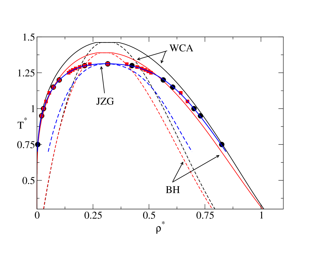
Figure 1:

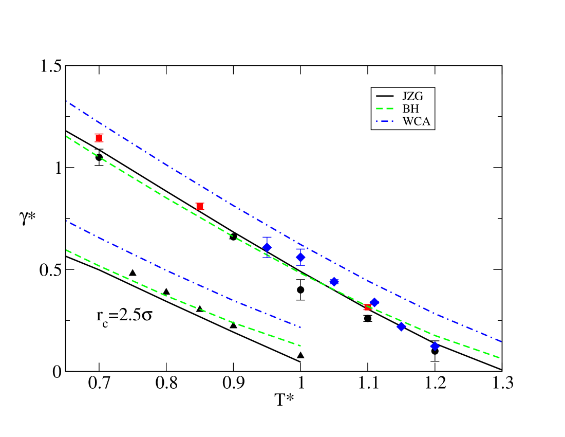
Figure 2:

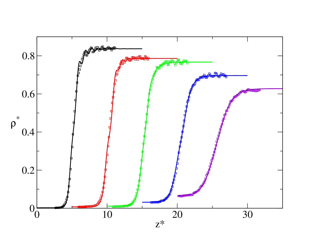
Figure 3:

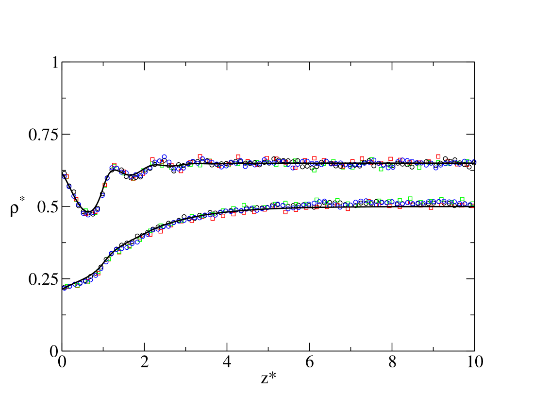
Figure 4:

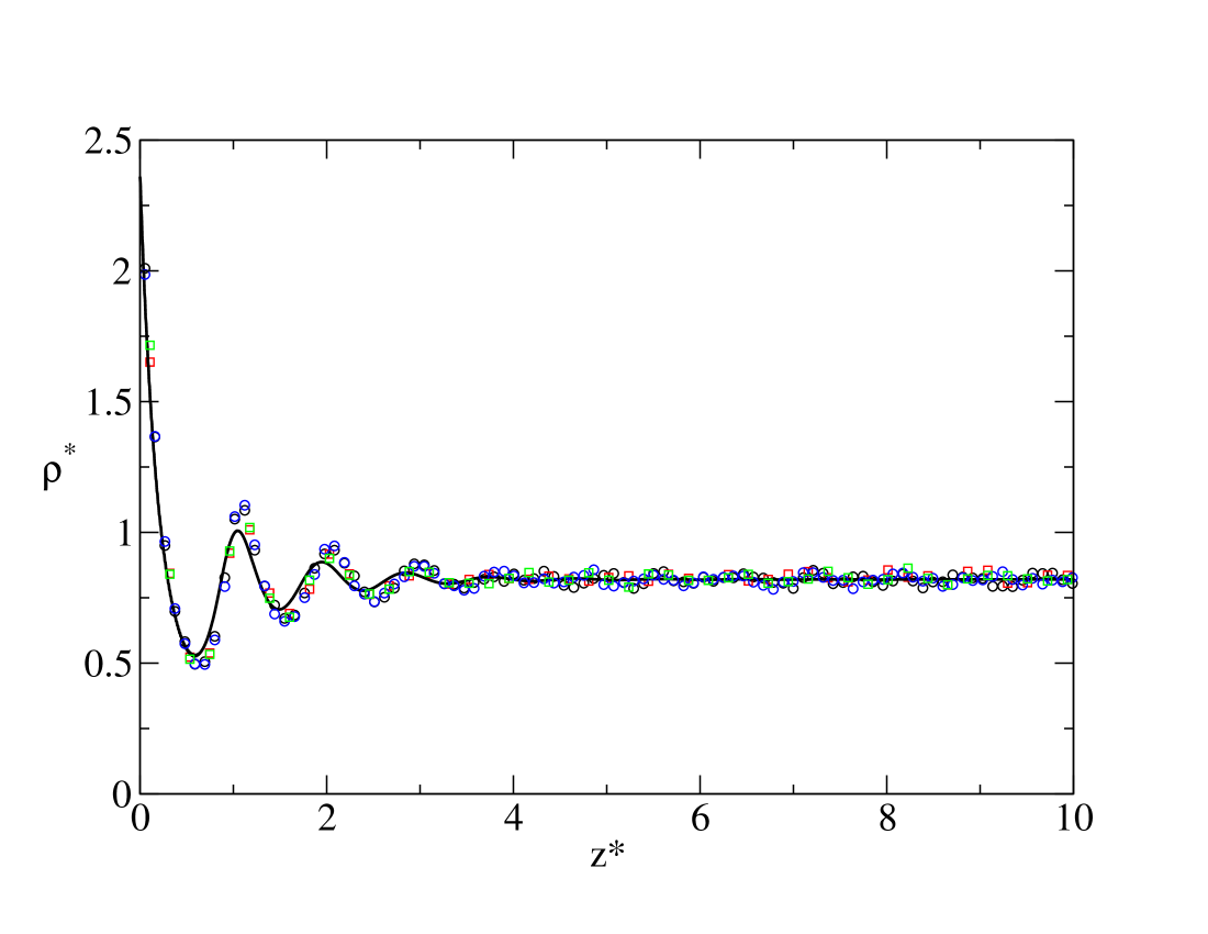
Figure 5:

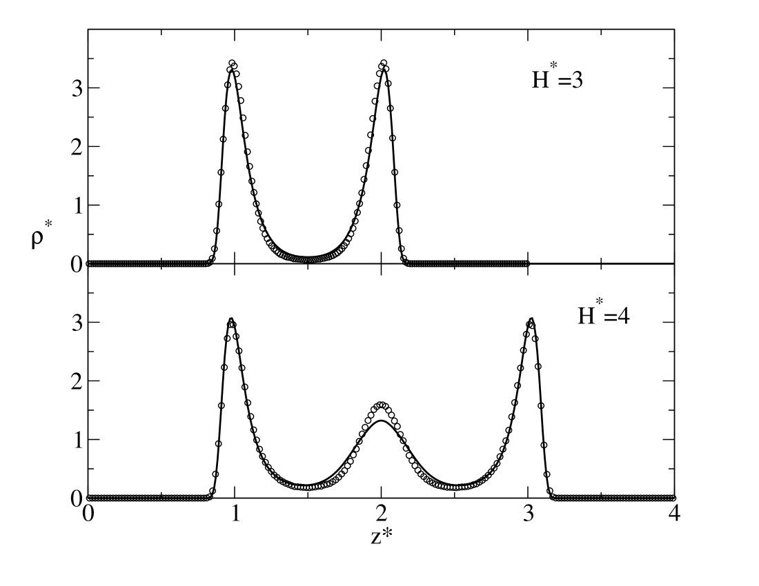
Figure 6:

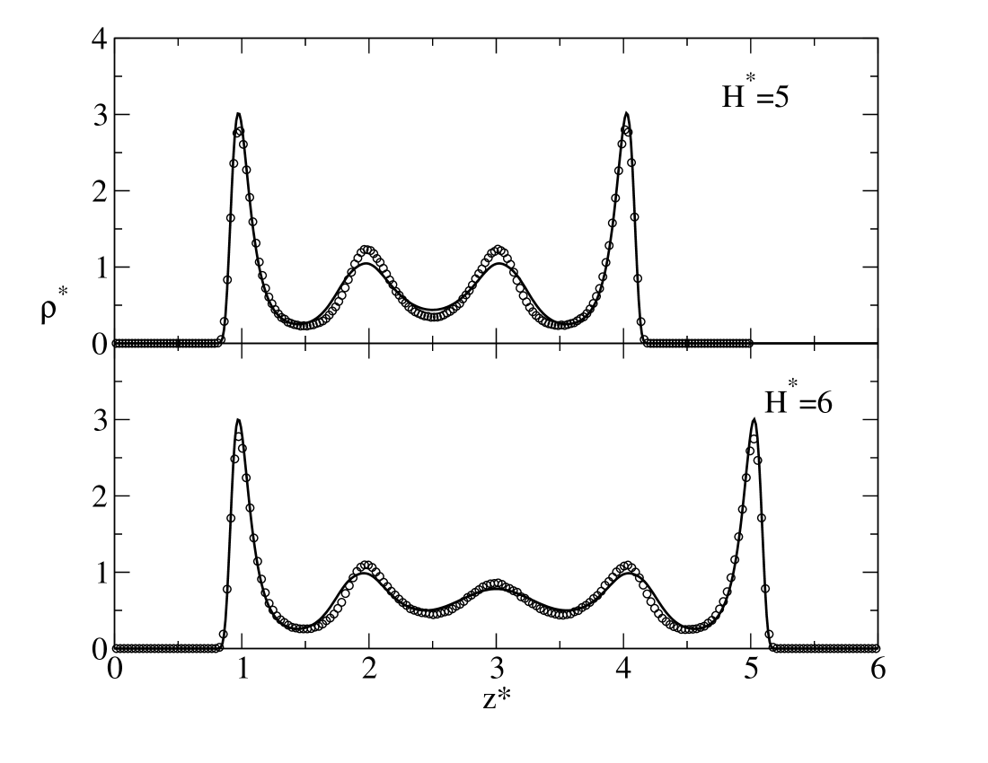
Figure 7:

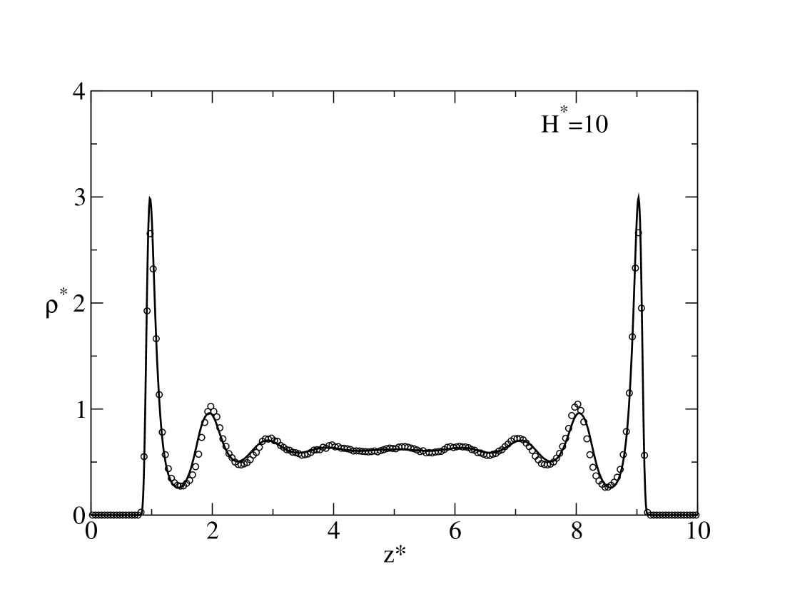
Figure 8:

References

- Rowlinson (1979) J. S. Rowlinson, J. Stat. Phys. 20, 197 (1979).
- van der Waals (1894) J. D. van der Waals, Z. Phys. Chem. 13, 657 (1894).
- Lutsko (2007) J. F. Lutsko, J. Chem. Phys. 127, 054701 (2007).
- Rosenfeld (1989) Y. Rosenfeld, Phys. Rev. Lett. 63, 980 (1989).
- Rosenfeld et al. (1990) Y. Rosenfeld, D. Levesque, and J.-J. Weis, J. Chem. Phys. 92, 6818 (1990).
- Kierlik and Rosinberg (1990) E. Kierlik and M. L. Rosinberg, Phys. Rev. A 42, 3382 (1990).
- Mermin (1965) N. D. Mermin, Phys. Rev. 137, A1441 (1965).
- Hansen and McDonald (1986) J.-P. Hansen and I. McDonald, Theory of Simple Liquids (Academic Press, San Diego, Ca, 1986).
- Johnson et al. (1993) J. K. Johnson, J. A. Zollweg, and K. E. Gubbins, Molecular Physics 78, 591 (1993).
- Barker and Henderson (1967) J. A. Barker and D. Henderson, J. Chem. Phys. 47, 4714 (1967).
- Chandler and Weeks (1970) D. Chandler and J. D. Weeks, Phys. Rev. Lett. 25, 149 (1970).
- Chandler et al. (1971) D. Chandler, J. D. Weeks, and H. C. Andersen, J. Chem. Phys. 54, 5237 (1971).
- Andersen et al. (1971) H. C. Andersen, D. Chandler, and J. D. Weeks, Phys. Rev. A 4, 1597 (1971).
- Roth et al. (2002) R. Roth, R. Evans, A. Lang, and G. Kahl, J. Phys.: Cond. Matt. 14, 12063 (2002).
- Tarazona (2002) P. Tarazona, Physica A 306, 243 (2002).
- Haye and Bruin (1994) M. J. Haye and C. Bruin, J. Chem. Phys. 100, 556 (1994).
- Mecke et al. (1997) M. Mecke, J. Winkelmann, and J. Fischer, J. Chem. Phys. 107, 9264 (1997).
- Katsov and Weeks (2002) K. Katsov and J. D. Weeks, J. Phys. Chem. B 106, 8429 (2002).
- Balabanic et al. (1989) C. Balabanic, B. Borstnik, R. Milcic, A. Rubcic, and F. Sokolic, in Static and Dynamic Properties of Liquids, edited by M. Davidoviv and A. K. Soper (Springer, Berlin, 1989), vol. 40 of Springer Proceedings in Physics.
- Tang et al. (1991) Z. Tang, L. E. Scriven, and H. T. Davis, J. Chem. Phys. 95, 2659 (1991).
- Frenkel and Smit (2001) D. Frenkel and B. Smit, Understanding Molecular Simulation (Academic Press, Inc., Orlando, FL, USA, 2001), ISBN 0122673514.
- Tang and Wu (2004) Y. Tang and J. Wu, Phys. Rev. E 70, 011201 (2004).
- Hendersen and Grundke (1975) D. Hendersen and E. W. Grundke, J. Chem. Phys. 63, 601 (1975).
- van Swol and Henderson (1989) F. van Swol and J. R. Henderson, Phys. Rev. A 40, 2567 (1989).
- Henderson (1992) D. Henderson, ed., Fundamentals of Inhomogeneous Fluids (Marcel Dekker Ltd, New York, 1992).
- Steele (1973) W. A. Steele, Surf. Sci. 36, 317 (1973).
- Steele (1974) W. A. Steele, The Interaction of Gases with Solid Surfaces (Pergamon, Oxford, 1974).
- Snook and van Megen (1980) I. K. Snook and W. van Megen, J. Chem. Phys. 72, 2907 (1980).
- van Megen and Snook (1981) W. J. van Megen and I. K. Snook, J. Chem. Phys. 74, 1409 (1981).
- Magda et al. (1985) J. J. Magda, M. Tirrell, and H. T. Davis, J. Chem. Phys. 83, 1888 (1985).
- Wadewitz and Winkelmann (2000) T. Wadewitz and J. Winkelmann, J. Chem. Phys. 113, 2447 (2000).
- Rogers and Young (1984) F. J. Rogers and D. A. Young, Phys. Rev. A 30, 999 (1984).
- Tang et al. (1997) Y. Tang, Z. Tong, and B. C.-Y. Lu, Fluid Phase Equilibria 134, 21 (1997).
- Tang and Wu (2003) Y. Tang and J. Wu, J. Chem. Phys. 119, 7388 (2003).
- Tang (2005) Y. Tang, J. Chem. Phys. 123, 204704 (2005).
- Rosenfeld et al. (1997) Y. Rosenfeld, M. Schmidt, H. Löwen, , and P. Tarazona, Phys. Rev. E 55, 4245 (1997).
- Tarazona (2000) P. Tarazona, Phys. Rev. Lett. 84, 694 (2000).
- Hansen and Verlet (1969) J. P. Hansen and L. Verlet, Phys. Rev. 184, 151 (1969).
- Potoff and Panagiotopoulos (2000) J. J. Potoff and A. Z. Panagiotopoulos, J. Chem. Physics 112, 6411 (2000).
- Duque et al. (2004) D. Duque, J. C. Pamies, and L. F. Vega, J. Chem. Phys. 121, 11395 (2004).
- Fischer (2007) J. Fischer, private communication (2007).