Linear conductance of an interacting carbon nanotube ring

Abstract

Linear transport through a single-walled carbon nanotube ring, pierced by a magnetic field and capacitively coupled to a gate voltage source, is investigated starting from a model of interacting $p_{z}$-electrons. The dc-conductance, calculated in the limit of weak tunneling between the ring and the leads, displays a periodic resonance pattern determined by the interplay between Coulomb interactions and quantum interference phenomena. Coulomb blockade effects are manifested in the absence of resonances for any applied flux in some gate voltage regions; the periodicity as a function of the applied flux can be smaller or larger than a flux quantum depending on the nanotube band mismatch.

I Introduction

Mesoscopic rings threaded by a magnetic field represent an important tool for the investigation of quantum interference phenomena. The archetype example is the well known Aharonov-Bohm effect Aharonov59 , where the conductance of a clean ring exhibits a periodicity of one flux quantum $\Phi_{0}=h/e$. However, impurities Altshuler81 and interactions Jagla93 can change this periodicity. In particular when transport through a one-dimensional ring is considered, interactions lead to spin-charge separation, such that the most important contribution to the conductance arises when both charge and spin excitations propagate from one contact to the other arriving at the drain at the same time Jagla93 . Additionally, the dc-conductance of an interacting one-dimensional ring shows Coulomb oscillations with peak positions depending on the applied magnetic field and interaction strength Kinaret98 ; Pletyukhov06 .

Among quasi-one dimensional systems, single-walled carbon nanotubes Saito98 (SWNTs) have been proved to be extremely interesting to probe electron-electron correlation effects. Luttinger liquid behavior, leading to power-law dependence of various quantities, has been predicted theoretically Egger97 ; Kane97 and observed experimentally Bockrath99 ; Tans97 ; Postma01 ; Lee04 in long, straight nanotubes.

Moreover, as typical of low-dimensional systems, short, straight carbon nanotubes weakly attached to leads exhibit Coulomb blockade at low temperatures Tans97 . In metallic SWNTs two bands cross at the Fermi energy. Together with the spin degree this leads to the formation of electron shells, each accommodating up to four electrons. As a result, a characteristic even-odd Cobden02 or fourfold Liang02 ; Sapmaz05 ; Moriyama05 periodicity of the Coulomb diamond size as a function of the gate voltage is found. Recently, spin-orbit effects in carbon nanotube quantum dots have been observed as well Kuemmeth08 . While the Coulomb blockade can be explained merely by the ground state properties of a SWNT, the determination of the current at higher bias voltages requires the inclusion of transitions of the system to electronic excitations. In Oreg00 a mean-field treatment of the electron-electron interactions has been invoked to calculate the energy spectrum, while in Mayrhofer06 a bosonization approach, valid for nanotubes with moderate-to-large diameters ($\emptyset>1.5$nm), has been used. Within the bosonization approach the fermionic ground state as well as the fermionic and bosonic excitations can be calculated. For small diameter nanotubes, short range interactions lead to pronounced exchange effects Oreg00 ; Mayrhofer08 which result in an experimentally detectable Moriyama05 singlet-triplet splitting.

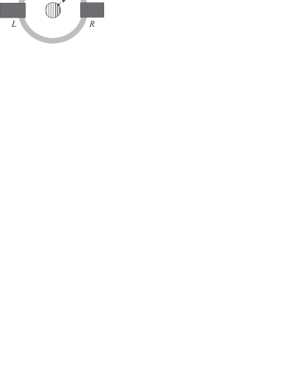
Figure 1: Top view of a SWNT ring contacted to extended left and right leads and threaded by a magnetic flux $\phi$. The ring is also capacitively coupled to a gate voltage $V_{g}$ plane situated beneath the ring (not shown).

Generically, nanotubes have linear or curved shape. Individual circular single-wall carbon nanotubes have been observed in Liu97 ; Martel99 ; Shea00 . However, these systems have been poorly experimentally investigated so far. Also from the theoretical point of view, only few works address the properties of toroidal nanotubes Lin98 ; Odinstov99 ; Rollb hler99 ; Latil03 ; Rocha04 ; Zaho04 ; Jack07 . Moreover, except for the studies Odinstov99 ; Rollb hler99 , on the persistent current and on the conductance of toroidal SWNTs, respectively, all the remaining theoretical works neglect electron-electron interactions effects. However, as for the case of straight SWNTs discussed above, electron correlation effects are expected to crucially influence the energy spectrum and transport properties of toroidal SWNTs. Indeed, in Odinstov99 it is found that for interacting SWNTs rings the persistent current pattern corresponds to the constant interaction model, with a fine structure stemming from exchange correlations. Results for the conductance of a SWNT ring weakly contacted to rings have been presented so far only in the short report Rollb hler99 , where a conductance resonance pattern depending on the interaction strength is reported. Moreover, a detailed derivation of the conductance formula for SWNT rings is missing in the short report Rollb hler99 . In this work we generalize the analysis of Kinaret98 on the conductance of interacting spinless electrons in a one-dimensional ring to the case of a three-dimensional toroidal, metallic SWNT at low energies. To this extent we start from a model of interacting $p_{z}$ electrons on a graphene lattice at low energies and impose periodic boundary conditions along the nanotube circumference and twisting boundary conditions along the tube axis. At low energies only the lowest transverse energy sub-bands of the ring contribute to transport, so that the problem becomes effectively one-dimensional in momentum space. The three-dimensional shape of the SWNT orbitals in real space, however, crucially determines the final conductance formula. Indeed, in contrast to Rollb hler99 , we find the absence of interference terms between anti-clockwise and clockwise circulating electrons in the conductance formula. This is due to the localized character of the $p_{z}$ orbitals and the fact that for a realistic nanotube the contacts are extended. Additionally, we predict an eight electron periodicity of the conductance resonance pattern as a function of the applied gate voltage. Coulomb blockade effects are clearly visible in that for some gate voltage ranges a resonance condition is not met for any value of the applied flux. The resonance pattern is also periodic as a function of the applied magnetic field, with a periodicity which can be larger or smaller than one flux quantum for nanotubes with a band mismatch.

The manuscript is organized as follows. The total Hamiltonian and its low energy spectrum are discussed in Secs. II and III. Specifically, the low energy Hamiltonian of the non-interacting system possesses two linear branches, corresponding to clockwise and anti-clockwise motion, crossing at the two non-equivalent Fermi points of the graphene lattice. By inclusion of the dominant forward scattering processes only, the interacting Hamiltonian is diagonalized exactly by standard bosonization techniques Delft98 . In IV the conductance formula is derived, while Sec. V is dedicated to the evaluation of the Green’s functions of the interacting SWNT ring. Finally the conductance resonance pattern is discussed in Sec. VI, where also conclusions are drawn.

II The total Hamiltonian

We consider a ring made of a toroidal metallic single-wall carbon nanotube coupled to a source and drain electrode via tunneling contacts, cf. figure 1. The torus is capacitively connected to a gate electrode with gate voltage $V_{g}$, which changes the chemical potential of the ring. Further, a magnetic flux $\phi$ threads the center of the torus. We wish to study how the two parameters $V_{g}$ and $\phi$ influence the linear conductance of the system. The model Hamiltonian reads

$$\hat{H}=\hat{H}_{\mathrm{ring}}+\hat{H}_{L}+\hat{H}_{R}+\hat{H}_{T}+\hat{H}_{ext},$$ (1)

where $\hat{H}_{\mathrm{ring}}$, which also includes the parameters $V_{g}$ and $\phi$, describes the physics of the isolated SWNT ring and will be discussed in the next section. The second and third term refer to the metallic left and right contacts, described here as Fermi gases of non-interacting electrons. They read ($\alpha=L/R$) $\hat{H}_{\alpha}=\sum_{{\vec{q}}\sigma}\varepsilon_{\alpha}(q)c^{\dagger}_{\alpha{\vec{q}}\sigma}c^{\phantom{\dagger}}_{\alpha{\vec{q}}\sigma}$, where $\varepsilon_{\alpha}(q)$ is the energy dispersion relation of the lead $\alpha$ and $c_{\alpha{\vec{q}}\sigma}$ is an operator annihilating an electron with wave vector ${\vec{q}}$ and spin $\sigma$.
The term $\hat{H}_{T}$ is the Hamiltonian describing tunneling between the ring and the leads. Therefore it consists of two terms, $\hat{H}_{T}=\hat{H}_{TL}+\hat{H}_{TR}$, and reads

$$\hat{H}_{T}=\sum_{\alpha=R,L}\sum_{\sigma}\int d^{3}r(T_{\alpha}(\vec{r})\Psi_{\sigma}^{\dagger}(\vec{r})\Phi_{\sigma\alpha}(\vec{r})+h.c.),$$ (2)

where $\Psi_{\sigma}^{\dagger}({\vec{r}})$ and $\Phi_{\sigma\alpha}(\vec{r})=\sum_{\vec{q}}\phi_{\vec{q}}(\vec{r})c_{{\vec{q}}\sigma\alpha}$ are electron operators in the dot and in the leads, respectively, and $T_{\alpha}(\vec{r})$ describes the generally position dependent transparency of the tunneling contact at lead $\alpha$. In the following we choose the representation where ${\vec{r}}=(x,r_{\perp})$, with $x$ being directed along the tube axis, while $r_{\perp}$ is the coordinate on the nanotube cross-section. With $L$ being the circumference of the SWNT ring, the contacts are positioned in the region about $x=0$ and $x=L/2$, see Fig. 1. Finally, ${\hat{H}}_{ext}$ accounts for the energy dependence of the system on the external voltage sources controlling the chemical potential in the leads: ${\hat{H}}_{ext}=-e\sum_{\alpha}V_{\alpha}\sum_{{\vec{q}}\sigma}c^{\dagger}_{\alpha{\vec{q}}\sigma}c_{\alpha{\vec{q}}\sigma}$.

III Low energy description of metallic SWNT rings

In this section we derive the low energy Hamiltonian $\hat{H}_{\mathrm{ring}}(\phi)=\hat{H}_{\rm kin}+\hat{V}_{\rm e-e}+\hat{H}_{\rm gate}$ of the SWNT ring and diagonalize it. The ring Hamiltonian includes a kinetic term, the electron-electron interactions as well as the effects of a capacitively applied gate voltage $V_{g}$ and of a magnetic flux $\phi$. We assume a metallic SWNT. Hence, depending on the diameter of the SWNT, ”low energies” means an energy range of the order of 1 eV around the Fermi energy, where the dispersion relation for the non-interacting electrons near the Fermi points is linear and only the two lowest subbands touching at the Fermi points can be considered. The effects of the magnetic field are included by introducing twisted boundary conditions (TBC) Loss93 . Curvature and Zeeman effects are neglected here. Indeed the Zeeman splitting yields a contribution inversely proportional to the the square of the ring radius Lin98 and is relevant only for very small rings. Finally, the linear dispersion relation around the Fermi points allows bosonization Delft98 of the interacting Hamiltonian and its successive diagonalization when only the forward scattering part of the Coulomb interaction is included. The latter approximation is justified for SWNTs with medium-to-large cross-sections ($\emptyset>1.5$nm) Mayrhofer08 .

III.1 Twisted boundary conditions

The band structure of non-interacting electrons in a SWNT ring is conveniently derived from the band structure of the $p_{z}$ electrons in a graphene lattice. Since each unit cell of the graphene lattice contains two carbon atoms, there are a valence and a conduction band touching at the corner points of the first Brillouin zone. Only two of these Fermi points, $\pm{\vec{K}}_{0}=\pm\frac{4\pi}{3\sqrt{3}a_{0}}\hat{e}_{x}$, are independent. Since SWNTs are graphene sheets rolled up into a cylinder, we can obtain the electronic properties of a SWNT by imposing quantization of the wave vector $\vec{k}=k_{\bot}\hat{e}_{\bot}+k_{||}\hat{e}_{||}$ around the tube waist, i.e., denoting the SWNT circumference with $L_{\bot}$, one finds $k_{\bot}=\frac{2\pi}{L_{\bot}}m,\ \ m=0,\pm 1,\pm 2\ldots\ ,$ which leads to the formation of several subbands labelled by $m$. We consider here only SWNTs of the armchair type, $\hat{e}_{x}=\hat{e}_{||}$, which are all metallic. In this case, only the two sub-bands touching at the Fermi points $\pm K_{0}\vec{e}_{x}$ are relevant.

Figure 2 shows the linear valence and conduction bands of an armchair SWNT. Corresponding to the direction of motion of the electrons, there are two branches $b=R,L$ with positive and negative slope, respectively.

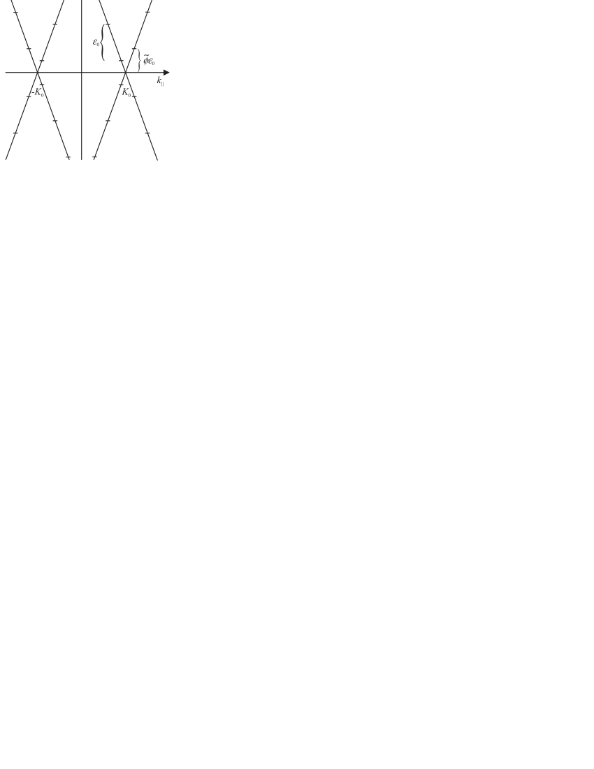
Figure 2: Low energy spectrum of a non-interacting SWNT ring threaded by a magnetic flux $\phi$. The underlying graphene structure is reflected in the two Fermi points at $\pm K_{0}$. Notice the misalignment $\tilde{\phi}\varepsilon_{0}$, with $\tilde{\phi}=\frac{\phi}{\phi_{0}}+\delta$, of the energy levels between the left ($L$) and right ($R$) branches due to the intrinsic mismatch $\delta$ and the applied flux $\phi$. The flux quantum is denoted $\phi_{0}$.

The linear dispersion relation reads

$$\varepsilon(b,\kappa)=\hbar v_{F}\mbox{sgn}(b)\kappa,$$ (3)

where $\kappa$ measures the distance between $k_{||}$ and the Fermi points $F=\pm K_{0}$, i.e., $k_{||}=\kappa+F$, and $v_{F}$ is the Fermi velocity, $v_{F}=8.1\times 10^{5}$m/s. Moreover, we use the convention $b=r/l=\pm 1$. The corresponding Bloch waves are of the form

$$\varphi_{Fb\kappa}(\vec{r}) = e^{i\kappa x}\varphi_{Fb}(\vec{r})$$

$$= e^{i\kappa x}\frac{1}{\sqrt{N_{L}}}\sum_{\vec{R},p}f_{pFb}e^{iFR_{x}}\Pi(\vec{r}-\vec{R}-\vec{\tau_{p}}).$$

Here, $N_{L}$ is the number of lattice points in the nanotube lattice. The index $p=1,2$ refers to the two graphene sublattices and $\vec{\tau}_{p}$ points from a lattice point $\vec{R}$ to a carbon atom of sublattice $p$. For an armchair SWNT, the parameters $f_{pFb}$ are found to be $f_{1Fb}=1/\sqrt{2},\ f_{2Fb}=-1/\sqrt{2}\mbox{ sgn}(Fb)$. Finally, we have the $p_{z}$ electron orbital $\Pi$.

As we consider a ring, we can impose in the absence of a magnetic field periodic boundary conditions along the direction parallel to the tube axis, yielding $k_{||}=\frac{2\pi}{L}m_{k}$, $m_{k}\in\mathbb{Z}$. As the Fermi points $\pm K_{0}$ are not necessarily an integer multiple of this step size, we introduce a mismatch parameter $\delta$, $\delta\in[-0.5,0.5)$, so that we can write $K_{0}=\frac{2\pi}{L}(n-\delta),\ \ n\in\mathbb{Z}.$ We still have to take account of the magnetic field. After travelling one time around the ring, an electron picks up a phase $2\pi\frac{\phi}{\phi_{0}}$, where $\phi_{0}=\frac{h}{e}$ is the flux quantum. This fact can be taken into account by introducing twisted boundary conditions (TBC), $\Psi(\vec{r}+L\hat{e}_{x})=e^{i2\pi\frac{\phi}{\phi_{0}}}\Psi(\vec{r})$ , instead of periodic ones Loss93 . Under TBC the allowed values of the momentum parallel to the tube axis $\kappa$ are

$$\kappa = \frac{2\pi}{L}\left(n_{\kappa}+\frac{\phi}{\phi_{0}}+\delta\right),\ n_{\kappa}\in\mathbb{Z}$$ (5)

$$\equiv \frac{2\pi}{L}\left(n_{\kappa}+\tilde{\phi}\right),\ m_{\kappa}\in\mathbb{Z}.$$

Thus the electron operator $\Psi$ including the electron spin $\sigma=\uparrow,\downarrow$ reads

$$\Psi(\vec{r}) = \sum_{\sigma}\Psi_{\sigma}(\vec{r})=\sum_{Fb\sigma\kappa}\varphi_{Fb\kappa}(\vec{r})c_{Fb\sigma\kappa}$$

$$= \sum_{Fb\sigma\kappa}e^{i\kappa x}\varphi_{Fb}(\vec{r})c_{Fb\sigma\kappa}\equiv\sqrt{L}\sum_{Fb\sigma}\varphi_{Fb}(\vec{r})\psi_{Fb\sigma}(x),$$

where $c_{Fb\sigma\kappa}$ annihilates an electron in state $\left|Fb\sigma\kappa\right\rangle$ and $\psi_{Fb\sigma}(x)$ is a slowly varying 1D operator. Later on the bosonisability of $\psi_{Fb\sigma}(x)$ will be of importance to evaluate the interference properties of the interacting SWNT ring.

III.2 Kinetic energy and gate Hamiltonian

The kinetic energy Hamiltonian in second quantization can in principle be read off from the dispersion relation for the low energy states (3):

$$\hat{H}_{\rm kin} = \hbar v_{F}\sum_{Fb\sigma\kappa}\mbox{sgn}(b)\kappa c^{\dagger}_{Fb\sigma\kappa}c^{\phantom{\dagger}}_{Fb\sigma\kappa}.$$ (7)

Inserting the $\kappa$-quantization (5), introducing the number counting operator $\mathcal{N}_{Fb\sigma}=\sum_{\kappa}c^{\dagger}_{Fb\sigma\kappa}c^{\phantom{\dagger}}_{Fb\sigma\kappa}$ and using the abbrevation $\varepsilon_{0}\equiv\hbar v_{F}\frac{2\pi}{L}$ we get

$$\hat{H}_{\rm kin} = \varepsilon_{0}\sum_{Fb\sigma}\mbox{sgn}(b)\left(\sum_{\kappa}m_{\kappa}c^{\dagger}_{Fb\sigma\kappa}c^{\phantom{\dagger}}_{Fb\sigma\kappa}+\tilde{\phi}\mathcal{N}^{\phantom{\dagger}}_{Fb\sigma}\right).$$

Gate voltage effects are included in the Hamiltonian ${\hat{H}}_{\rm gate}=-\mu_{\rm g}{\cal N}=-e\alpha V_{\rm g}$, where ${\cal N}=\sum_{Fb\sigma}\mathcal{N}^{\phantom{\dagger}}_{Fb\sigma}$ is the total electron operator of the SWNT, $\mu_{\rm g}$ is the SWNT chemical potential and $\alpha$ a conversion factor.

III.3 Interaction Hamiltonian

A general form of the Hamiltonian ${\hat{V}}_{\rm e-e}$ describing interactions between the electrons is

$${\hat{V}}_{\rm e-e}=\frac{1}{2}\sum_{\sigma\sigma^{\prime}}$$

$$\times \int d^{3}r\int d^{3}r^{\prime}\Psi^{\dagger}_{\sigma}(\vec{r})\Psi^{\dagger}_{\sigma^{\prime}}(\vec{r}\,^{\prime})U(\vec{r}-\vec{r}\,^{\prime})\Psi^{\phantom{\dagger}}_{\sigma^{\prime}}(\vec{r}\,^{\prime})\Psi^{\phantom{\dagger}}_{\sigma}(\vec{r}),$$

where $U(\vec{r}-\vec{r}\,^{\prime})$ is the possibly screened Coulomb potential. By expressing the 3D electron operator in terms of the 1D one, cf. Eq. (LABEL:el_op), and integrating over the components of $\vec{r}$ and $\vec{r}\,^{\prime}$ perpendicular to the tube axis one obtains an effective one-dimensional interaction. As discussed in Egger97 , this yields in general interlattice and intralattice interactions. In Mayrhofer08 it is shown that when the tube diameter is large enough, the distinction between intra and inter-lattice interactions is no longer relevant, and only forward scattering processes, where the number of electrons in each branch remains constant, are relevant.

Introducing the 1D electron density operator $\rho^{\phantom{\dagger}}_{Fb\sigma}(x)=\psi^{\dagger}_{Fb\sigma}(x)\psi^{\phantom{\dagger}}_{Fb\sigma}(x)$ and retaining only forward scattering processes we obtain for the interaction Hamiltonian

$${\hat{V}}_{\rm e-e} \approx \frac{1}{2}\sum_{FF^{\prime}}\sum_{bb^{\prime}}\sum_{\sigma\sigma^{\prime}}\int_{0}^{L}dx\int_{0}^{L}dx^{\prime}$$ (10)

$$\times \rho_{Fb\sigma}(x)V_{0}(x,x^{\prime})\rho_{F^{\prime}b^{\prime}\sigma^{\prime}}(x^{\prime}),$$

with the effective 1D potential $V_{0}(x,x^{\prime})$ defined as

$$V_{0}(x,x^{\prime})=\frac{L^{2}}{N_{L}^{2}}\sum_{\vec{R},\vec{R^{\prime}}}\int d^{2}r_{\bot}\int d^{2}r^{\prime}_{\bot}\times$$ (11)

$$\times |\Pi(\vec{r}-\vec{R})|^{2}U(\vec{r}-\vec{r}\,^{\prime})|\Pi(\vec{r}\,^{\prime}-\vec{R^{\prime}})|^{2}.$$

III.4 Bosonization

The problem of a one-dimensional system of interacting electrons is often conveniently formulated in terms of bosonic operators. A didactic overview can be found in Delft98 . To this extent we assume a linear dispersion relation over all values of the momentum $\kappa$. This is justified by the long-range character of the interaction, leading to a momentum cut-off still lying in the low-energy range around the Fermi energy. The states with negative energy are assumed to be filled in the ground state, the Fermi sea, of the system. As in Delft98 , we now introduce new bosonic operators

$$b_{F\sigma q} := \frac{1}{\sqrt{|n_{q}|}}\left\{\begin{array}[]{c}\sum_{\kappa}c^{\dagger}_{Fr\sigma\kappa}c^{\phantom{\dagger}}_{Fr\sigma\kappa+q},\ \ \ q>0\phantom{,}\\ \sum_{\kappa}c^{\dagger}_{Fl\sigma\kappa}c^{\phantom{\dagger}}_{Fl\sigma\kappa+q},\ \ \ q<0,\end{array}\right.$$ (14)

with $q=\frac{2\pi}{L}n_{q},n_{q}\in\mathbb{Z}$, and obeying the canonical bosonic commutation relations

$$[b^{\phantom{\dagger}}_{F_{1}\sigma_{1}q_{1}},b^{\dagger}_{F_{2}\sigma_{2}q_{2}}]=\delta_{F_{1}F_{2}}\delta_{\sigma_{1}\sigma_{2}}\delta_{q_{1}q_{2}},\ [b^{\phantom{\dagger}}_{F_{1}\sigma_{1}q_{1}},b^{\phantom{\dagger}}_{F_{2}\sigma_{2}q_{2}}]=0.$$

In terms of the bosonic operators (14) the kinetic energy Hamiltonian (LABEL:kin_energy) assumes the form

$$\hat{H}_{\mathrm{kin}} := \varepsilon_{0}\sum_{F\sigma}\sum_{q\neq 0}|n_{q}|b^{\dagger}_{F\sigma q}b^{\phantom{\dagger}}_{F\sigma q}+$$ (16)

$$+ \varepsilon_{0}\sum_{Fb\sigma}\left[\frac{\mathcal{N}^{2}_{Fb\sigma}}{2}+\tilde{\phi}\,\mbox{sgn}(b)\mathcal{N}_{Fb\sigma}\right].$$

For the bosonization of the interaction part (10), we decompose the density operator $\rho_{Fb\sigma}$ into its Fourier components, which are proportional to the bosonic operators (14):

$$\rho^{\phantom{\dagger}}_{Fb\sigma}(x)=\psi^{\dagger}_{Fb\sigma}(x)\psi^{\phantom{\dagger}}_{Fb\sigma}(x)=\mathcal{N}_{Fb\sigma}$$ (17)

$$+\sum_{q>0}\sqrt{|n_{q}|}\left(e^{i\mbox{\scriptsize sgn}(b)qx}b^{\phantom{\dagger}}_{F\sigma\mbox{\scriptsize sgn}(b)q}+e^{-i\mbox{\scriptsize sgn}(b)qx}b^{\dagger}_{F\sigma\mbox{\scriptsize sgn}(b)q}\right).$$

By inserting (17) into (10) we get

$$\hat{V} = \frac{1}{2}W_{00}\mathcal{N}^{2}+\sum_{F\sigma}\sum_{F^{\prime}\sigma^{\prime}}\sum_{q\neq 0}\frac{1}{2}W_{q-q}|n_{q}|\times$$

$$\times \left(b^{\phantom{\dagger}}_{F\sigma q}+b^{\dagger}_{F\sigma-q}\right)\left(b^{\phantom{\dagger}}_{F^{\prime}\sigma^{\prime}-q}+b^{\dagger}_{F^{\prime}\sigma^{\prime}q}\right),$$

with the total number of electrons $\mathcal{N}=\sum_{Fb\sigma}\mathcal{N}_{Fb\sigma}$ in the ring. The effective interaction $V_{0}(x,x^{\prime})$ is absorbed into

$$W_{qq^{\prime}} \equiv \int_{0}^{L}dx\int_{0}^{L}dx^{\prime}e^{i(qx+q^{\prime}x^{\prime})}V_{0}(x,x^{\prime}).$$ (18)

This is nonzero only for $q^{\prime}=-q$ and yields

$$W_{q-q}=L\cdot\int_{-L/2}^{L/2}dy\cos(qy)V_{0}(|y|).$$ (19)

The parameter $W_{00}$ can be identified with the charging energy $E_{c}$ responsible for Coulomb blockade. To proceed, it is convenient to introduce linear combinations of the bosonic operators (14) associated to spin, charge and orbital degrees of freedom:

$$b_{\oplus cq} := \frac{1}{2}(b_{K_{0}\uparrow q}+b_{K_{0}\downarrow q}+b_{-K_{0}\uparrow q}+b_{-K_{0}\downarrow q}),$$

$$b_{\ominus cq} := \frac{1}{2}(b_{K_{0}\uparrow q}+b_{K_{0}\downarrow q}-b_{-K_{0}\uparrow q}-b_{-K_{0}\downarrow q}),$$

$$b_{\oplus sq} := \frac{1}{2}(b_{K_{0}\uparrow q}-b_{K_{0}\downarrow q}+b_{-K_{0}\uparrow q}-b_{-K_{0}\downarrow q}),$$

$$b_{\ominus sq} := \frac{1}{2}(b_{K_{0}\uparrow q}-b_{K_{0}\downarrow q}-b_{-K_{0}\uparrow q}+b_{-K_{0}\downarrow q}),$$

or shortly: $b_{\tilde{F}jq}$, $\tilde{F}=\oplus/\ominus$, $j=c,s$. The advantage of this transformation is that the term quadratic in the bosonic operators in $\hat{V}_{\rm e-e}$ contains now only $b_{\oplus cq}$-type operators. The ring Hamiltonian finally reads

$$\hat{H}_{\mathrm{ring}}=\varepsilon_{0}\sum_{\tilde{F}j}\sum_{q\neq 0}|n_{q}|b^{\dagger}_{\tilde{F}jq}b^{\phantom{\dagger}}_{\tilde{F}jq}-\mu_{\rm g}{\cal N}$$

$$+ \varepsilon_{0}\sum_{Fb\sigma}\left(\frac{\mathcal{N}^{2}_{Fb\sigma}}{2}+\tilde{\phi}\,\mbox{sgn}(b)\mathcal{N}_{Fb\sigma}\right)+\frac{1}{2}W_{00}\mathcal{N}^{2}$$

$$+ \frac{1}{2}\sum_{q\neq 0}4|n_{q}|W_{q-q}\left(b^{\phantom{\dagger}}_{\oplus cq}+b^{\dagger}_{\oplus c-q}\right)\left(b^{\phantom{\dagger}}_{\oplus c-q}+b^{\dagger}_{\oplus cq}\right).$$

III.4.1 Diagonalization

The Hamiltonian (LABEL:V_boson_sc) can be diagonalized by a Bogoliubov transformation. More details can be found in the Appendix. As a result we get

$$\hat{H}_{\mathrm{ring}}=\sum_{\tilde{F}j}\sum_{q\neq 0}\varepsilon_{\tilde{F}jq}a_{\tilde{F}jq}^{\dagger}a^{\phantom{\dagger}}_{\tilde{F}jq}+\varepsilon_{0}\sum_{Fb\sigma}\frac{\mathcal{N}^{2}_{Fb\sigma}}{2}$$ (21)

$$+ \varepsilon_{0}\tilde{\phi}\sum_{Fb\sigma}\mbox{sgn}(b)\mathcal{N}_{Fb\sigma}+\frac{1}{2}W_{00}\mathcal{N}^{2}-\mu_{\rm g}{\cal N}.\;$$

The definition of the energies $\varepsilon_{\tilde{F}jq}$ as well as the relation between the new ($a_{\tilde{F}jq}$) and the old ($b_{\tilde{F}jq}$) operators can be found in the Appendix. The degrees of freedom which are affected by the interaction are those related to the $a_{\oplus cq}$-operators. Therefore, these are called charged degrees of freedom, whereas the indices $(\ominus cq)$, $(\oplus sq)$ and $(\ominus sq)$ denote the neutral modes. In total, there are one charged and three neutral modes.
In order to investigate the combined effects of gate voltage and magnetic flux, it is convenient to introduce appropriate linear combinations of the number counting operator $\mathcal{N}_{Fr\sigma}$ :

$$\mathcal{N} \equiv \mathcal{N}_{\oplus c}:=\sum\limits_{Fb\sigma}\mathcal{N}_{Fb\sigma},$$

$$\mathcal{J} \equiv \mathcal{J}_{\oplus c}:=\sum\limits_{Fb\sigma}\mbox{sgn}(b)\mathcal{N}_{Fb\sigma},$$ (22)

being the total particle and total current operators and

$$\mathcal{N}_{\oplus s} := \sum\limits_{Fb\sigma}\mbox{sgn}(\sigma)\mathcal{N}_{Fb\sigma},\qquad\mathcal{J}_{\oplus s}:=\sum\limits_{Fb\sigma}\mbox{sgn}(b\sigma)\mathcal{N}_{Fb\sigma},$$

$$\mathcal{N}_{\ominus c} := \sum\limits_{Fb\sigma}\mbox{sgn}(F)\mathcal{N}_{Fb\sigma},\qquad\mathcal{J}_{\ominus c}:=\sum\limits_{Fb\sigma}\mbox{sgn}(Fb)\mathcal{N}_{Fb\sigma},$$

$$\mathcal{N}_{\ominus s} := \sum\limits_{Fb\sigma}\mbox{sgn}(F\sigma)\mathcal{N}_{Fb\sigma},\quad\mathcal{J}_{\ominus s}:=\sum\limits_{Fb\sigma}\mbox{sgn}(Fb\sigma)\mathcal{N}_{Fb\sigma}.$$

Expressing $\hat{H}_{\mathrm{ring}}$ in terms of these newly defined operators yields

$$\hat{H}_{\mathrm{ring}} := \hat{H}_{\mathrm{ring,b}}+\hat{H}_{\mathrm{ring,f}}=\sum_{\tilde{F}j}\sum_{q\neq 0}\varepsilon^{\phantom{\dagger}}_{\tilde{F}jq}a_{\tilde{F}jq}^{\dagger}a^{\phantom{\dagger}}_{\tilde{F}jq}$$ (23)

$$+ \frac{\varepsilon_{0}}{16}[\tilde{W}({\mathcal{N}}-k_{\mu_{g}})^{2}+({\mathcal{J}}-k_{\phi})^{2}]$$

$$+ \frac{\varepsilon_{0}}{16}\sum_{\tilde{F}j\neq\oplus c}(\mathcal{N}^{2}_{\tilde{F}j}+\mathcal{J}^{2}_{\tilde{F}j})+{\rm const},$$

where $\tilde{W}=1+\frac{8W_{00}}{\varepsilon_{0}}$, $k_{\mu_{g}}=\frac{\mu_{g}}{W_{00}+\varepsilon_{0}/8}$ and $k_{\phi}=-8\tilde{\phi}$. The first line corresponds to the bosonic part of the Hamiltonian, $\hat{H}^{\phantom{\dagger}}_{\mathrm{ring,b}}$ and the second and third lines to the fermionic part $\hat{H}^{\phantom{\dagger}}_{\mathrm{ring,f}}$. An eigenbasis of $\hat{H}_{\rm ring}$ is thus formed by the states

$$\left\{\prod_{\tilde{F}j,q\neq 0,}\frac{(a^{\dagger}_{\tilde{F}jq})^{m_{\tilde{F}jq}}}{\sqrt{m_{\tilde{F}jq}!}}\left|\vec{N}\right\rangle\right\}=:\left\{\left|\vec{N},\vec{m}\right\rangle\right\},$$ (24)

where $\left|\vec{N},\vec{0}\right\rangle$ has no bosonic excitations. In general, any number of electrons can be distributed in many different ways on the branches $(Fb\sigma)$, which is described by the set of vectors

$$\vec{N} = (N_{K_{0}r\uparrow},N_{K_{0}r\downarrow},N_{K_{0}l\uparrow},N_{K_{0}l\downarrow},$$ (25)

$$N_{-K_{0}r\uparrow},N_{-K_{0}r\downarrow},N_{-K_{0}l\uparrow},N_{-K_{0}l\downarrow}).$$

For each value of $\vec{N}$ one has to include the states which contain the bosonic excitations of the interacting electrons, where the the parameter $m_{\tilde{F}jq}$ counts the number of excitations in the channel $\tilde{F}j$ with momentum $q$.

IV Linear transport

We have now all the ingredients to evaluate the linear transport characteristics of the interacting SWNT ring by use of the Kubo formula.

IV.1 Conductance formula

The current operator at lead $L$ is defined as the rate of change of particles at the contact $L$, i.e., $\hat{I}_{L}=-e{\dot{\hat{N}}}_{L}=-\frac{ie}{\hbar}[\hat{H},\hat{N}_{L}]=-\frac{ie}{\hbar}[\hat{H}_{TL},\hat{N}_{L}]$ where $-e$ is the electron charge. It yields

$$\hat{I}_{L}=-\frac{ie}{\hbar}\sum_{\sigma}\int d^{3}r(T_{L}(\vec{r})\Psi_{\sigma}^{\dagger}(\vec{r})\Phi_{\sigma L}(\vec{r})-h.c.).$$ (26)

Analogously the current operator at the right lead is

$$\hat{I}_{R}=\frac{ie}{\hbar}\sum_{\sigma}\int d^{3}r(T_{R}(\vec{r})\Psi_{\sigma}^{\dagger}(\vec{r})\Phi_{\sigma R}(\vec{r})-h.c.).\;$$ (27)

To proceed, we use relation (LABEL:el_op), relating the 3D operator $\Psi(\vec{r})$ to the slowly varying 1D one $\psi_{Fb\sigma}(x)$. We assume that the latter does not change significantly in the tunneling region. This yields for the current operators

$$\hat{I}_{L}=-\frac{ie}{\hbar}\sum_{Fb\sigma}\sum_{\vec{q}}\times$$ (28)

$$\Biggl{(}\underbrace{\sqrt{L}\int d^{3}rT_{L}(\vec{r})\varphi^{*}_{Fb}(\vec{r})\phi_{\vec{q},L}(\vec{r})}_{=:T_{LFb\vec{q}}}\psi_{Fb\sigma}^{\dagger}(x_{L})c_{\vec{q}\sigma L}-h.c.\Biggr{)}$$

$$= -\frac{ie}{\hbar}\sum_{Fb\sigma}\sum_{\vec{q}}\Biggl{(}T_{LFb\vec{q}}\psi_{Fb\sigma}^{\dagger}(x_{L})c_{\vec{q}\sigma L}-h.c.\Biggr{)},$$

$$\hat{I}_{R} = \frac{ie}{\hbar}\sum_{Fb\sigma}\sum_{\vec{q}}\Biggl{(}T_{RFb\vec{q}}\psi_{Fb\sigma}^{\dagger}(x_{R})c_{\vec{q}\sigma L}-h.c.\Biggr{)},$$ (29)

where $x_{L}$ and $x_{R}$ are in the middle of the respective tunneling regions. The above expressions for the current operators can in turn be used to evaluate the DC-conductance of the interacting SWNT ring in terms of the Kubo formula

$$G=\lim_{\Omega\rightarrow 0}\mbox{Re}\frac{1}{\hbar\Omega}\int_{-\infty}^{t}dt^{\prime}e^{i\Omega(t^{\prime}-t)}\langle[\hat{I}_{L}(t),\ \hat{I}_{R}(t^{\prime})]\rangle_{\rm eq},$$ (30)

with $\hat{I}_{L}(t)$ and $\hat{I}_{R}(t)$ being current operators in the interaction representation, where the interaction is represented by the Hamiltonian ${\hat{H}}_{ext}$. Hence, $\langle\quad\rangle_{\rm eq}$ describes the average with respect to the equilibrium density operator ${\hat{\rho}}_{\rm eq}:=Z^{-1}e^{-\beta({{\hat{H}}_{\rm ring}+{\hat{H}}_{T}+{\hat{H}}_{L}+{\hat{H}}_{R}})}$, with $\beta$ the inverse temperature and $Z$ the partition function. It is convenient to introduce the linear susceptibility $\chi(t)=-\frac{i}{\hbar}\theta(t)\langle[\hat{I}_{L}(t),\ \hat{I}_{R}(0)]\rangle_{\rm eq}$ in terms of which (30) assumes the compact form

$$G=\frac{1}{\hbar}\lim_{\Omega\rightarrow 0}i\frac{\tilde{\chi}(\Omega)}{\Omega}.$$ (31)

Here $\tilde{\chi}(\Omega)$ is the Fourier transform of the response function $\chi(t)$. In Kinaret98 the linear susceptibility at imaginary times

$$\chi(\tau_{1}-\tau_{2})=-\langle T_{\tau}[\hat{I}_{L}(\tau_{1}),\hat{I}_{R}(\tau_{2})]\rangle_{\rm eq},$$ (32)

where $T_{\tau}$ indicates time-ordering, has been evaluated for a spinless Luttinger liquid. Generalizing Kinaret98 to the multichannel situation represented by a 3D toroidal SWNT, an expression for the linear susceptibility can be obtained to lowest non vanishing order in the tunneling matrix elements $T_{\alpha Fb\vec{q}}$. A summary of the calculation, where we made use of the explicit form of the nanotube Bloch wave functions, can be found in the subsection below. It delivers for the conductance the remarkably simple result

$$G \approx \frac{e^{2}}{h}\frac{|\Phi_{L}|^{2}|\Phi_{R}|^{2}}{\hbar^{2}}$$

$$\times \sum_{Fb\sigma}\int_{-\infty}^{+\infty}d\omega\Biggl{(}-\frac{\partial n_{\rm F}(\omega)}{\partial\omega}\Biggr{)}|G^{\rm ret}_{Fb\sigma}(\omega,x_{L}-x_{R})|^{2},$$

where $n_{\rm F}(\omega)$ is the Fermi function and $G^{\rm ret}_{Fb\sigma}(\omega,x_{L}-x_{R})$, the retarded Green’s function for the interacting electrons on the SWNT ring, is entirely determined by the slowly varying 1D part of the electron operator (LABEL:el_op) as it is the Fourier transform of

$$G^{\rm ret}_{Fb\sigma}(t,{x}-{x}\,^{\prime}) = -\frac{i}{\hbar}\theta(t)\left\langle\{\psi_{Fb\sigma}({x},t),\psi^{\dagger}_{Fb\sigma}({x}\,^{\prime},0)\}\right\rangle.$$

As the number $\cal N$ of electrons in the dot can vary, $\langle\ \rangle$ indicates the thermal average with respect to the grandcanonical equilibrium density matrix $\rho_{{\rm ring},{\cal N}}=Z^{-1}_{\rm ring}\exp^{-\beta\hat{H}_{\rm ring}}$. In contrast, knowledge of the 3D character of the SWNT Bloch wave functions is encapsulated in the tunneling functions $\Phi_{R}$ and $\Phi_{L}$, see Eq. (44) below. We notice that Eq. (IV.1) is not trivial, as it predicts the absence of interference between Green’s functions with different indices, in contrast to the case of a strictly one-dimensional ring considered in Kinaret98 and the formula given in Rollb hler99 . This result has its origin in the very strongly localized character of the $p_{z}$ orbitals, and on the fact that we assumed extended contacts coupling equally to both sublattices of the underlying graphene structure. For temperatures further than $k_{B}T$ from a resonance (IV.1) further simplifies to

$$G\approx\frac{e^{2}}{h}\frac{|\Phi_{L}|^{2}|\Phi_{R}|^{2}}{\hbar^{2}}\sum_{Fb\sigma}|G^{\rm ret}_{Fb\sigma}(0,x_{L}-x_{R})|^{2}.$$ (35)

IV.2 Proof of the conductance formula (IV.1)

In this subsection, which the hurried reader can skip, the linear susceptibility $\tilde{\chi}(\Omega)$ entering the conductance formula (31) is obtained by first evaluating the Fourier transform $\tilde{\chi}(i\Omega_{n})$ of the imaginary time response function $\chi(\tau)$ and successive analytic continuation: $\tilde{\chi}(\Omega)=\lim_{i\Omega_{n}\to\Omega}\tilde{\chi}(i\Omega_{n})$. Specifically, we use the generating function method to find an expression for the imaginary time susceptibility at lowest order in the tunneling couplings Kinaret98 . It reads

$$\chi(\tau_{1}-\tau_{2})=-\frac{e^{2}}{\hbar^{4}}\int_{0}^{\hbar\beta}d\tau\int_{0}^{\hbar\beta}d\tau^{\prime}\sum_{F_{1}b_{1}}\sum_{F_{2}b_{2}}\sum_{F_{3}b_{3}}\sum_{F_{4}b_{4}}\sum_{\sigma\sigma^{\prime}}\sum_{\vec{q}\vec{q}^{\prime}}T_{LF_{1}b_{1}\vec{q}}T^{*}_{LF_{2}b_{2}\vec{q}}T_{RF_{3}b_{3}\vec{q}^{\prime}}T^{*}_{RF_{4}b_{4}\vec{q}^{\prime}}\times$$

$$\times\Bigl{\{}\langle T_{\tau}\left[\psi^{\dagger}_{F_{1}b_{1}\sigma}(\tau,x_{L})\psi_{F_{2}b_{2}\sigma}(\tau_{1},x_{L})\psi^{\dagger}_{F_{3}b_{3}\sigma^{\prime}}(\tau^{\prime},x_{R})\psi_{F_{4}b_{4}\sigma^{\prime}}(\tau_{2},x_{R})\right]\rangle G_{L\sigma}(\vec{q},\tau-\tau_{1})G_{R\sigma}(\vec{q}^{\prime},\tau^{\prime}-\tau_{2})+$$

$$\phantom{\ }-\langle T_{\tau}\left[\psi^{\dagger}_{F_{1}b_{1}\sigma}(\tau,x_{L})\psi_{F_{2}b_{2}\sigma}(\tau_{1},x_{L})\psi^{\dagger}_{F_{3}b_{3}\sigma^{\prime}}(\tau_{2},x_{R})\psi_{F_{4}b_{4}\sigma^{\prime}}(\tau^{\prime},x_{R})\right]\rangle G_{L\sigma}(\vec{q},\tau-\tau_{1})G_{R\sigma}(\vec{q}^{\prime},\tau_{2}-\tau^{\prime})+$$

$$\phantom{\ }-\langle T_{\tau}\left[\psi^{\dagger}_{F_{1}b_{1}\sigma}(\tau_{1},x_{L})\psi_{F_{2}b_{2}\sigma}(\tau,x_{L})\psi^{\dagger}_{F_{3}b_{3}\sigma^{\prime}}(\tau^{\prime},x_{R})\psi_{F_{4}b_{4}\sigma^{\prime}}(\tau_{2},x_{R})\right]\rangle G_{L\sigma}(\vec{q},\tau_{1}-\tau)G_{R\sigma}(\vec{q}^{\prime},\tau^{\prime}-\tau_{2})+$$

$$\phantom{\ }+\left.\langle T_{\tau}\left[\psi^{\dagger}_{F_{1}b_{1}\sigma}(\tau_{1},x_{L})\psi_{F_{2}b_{2}\sigma}(\tau,x_{L})\psi^{\dagger}_{F_{3}b_{3}\sigma^{\prime}}(\tau_{2},x_{R})\psi_{F_{4}b_{4}\sigma^{\prime}}(\tau^{\prime},x_{R})\right]\rangle G_{L\sigma}(\vec{q},\tau_{1}-\tau)G_{R\sigma}(\vec{q}^{\prime},\tau_{2}-\tau^{\prime})\right\},$$ (36)

where $G_{\alpha\sigma}(\vec{q},\tau-\tau^{\prime})=-\langle T_{\tau}(c_{\vec{q}\sigma\alpha}(\tau)c^{\dagger}_{\vec{q}\sigma\alpha}(\tau^{\prime}))\rangle_{\alpha}$ denotes the Green’s function for the free electrons of lead $\alpha$. In (36) $\langle\quad\rangle_{\alpha}$ describes the average with respect to the equilibrium density operator $Z^{-1}_{\alpha}e^{-\beta{\hat{H}}_{\alpha}}$ of the lead $\alpha$.

Though the four particles correlator can in principle be evaluated using the bosonisation approach, see e.g. Pletyukhov06 , following Kinaret98 we factorize it as

$$\langle T_{\tau}\psi^{\dagger}_{F_{1}b_{1}\sigma}(\tau,x_{L})\psi_{F_{2}b_{2}\sigma}(\tau_{1},x_{L})\psi^{\dagger}_{F_{3}b_{3}\sigma^{\prime}}(\tau^{\prime},x_{R})\psi_{F_{4}b_{4}\sigma^{\prime}}(\tau_{2},x_{R})\rangle$$ (37)

$$\approx \delta_{F_{1}F_{2}}\delta_{b_{1}b_{2}}\delta_{F_{3}F_{4}}\delta_{b_{3}b_{4}}\langle T_{\tau}\psi_{F_{2}b_{2}\sigma}(\tau_{1},x_{L})\psi^{\dagger}_{F_{1}b_{1}\sigma}(\tau,x_{L})\rangle\langle\psi_{F_{4}b_{4}\sigma^{\prime}}(\tau_{2},x_{R})\psi^{\dagger}_{F_{3}b_{3}\sigma^{\prime}}(\tau^{\prime},x_{R})\rangle$$

$$- \delta_{F_{2}F_{3}}\delta_{b_{2}b_{3}}\delta_{F_{4}F_{1}}\delta_{b_{2}b_{3}}\delta_{\sigma\sigma^{\prime}}\langle T_{\tau}\psi_{F_{2}r_{2}\sigma}(\tau_{1},x_{L})\psi^{\dagger}_{F_{3}b_{3}\sigma^{\prime}}(\tau^{\prime},x_{R})\rangle\langle\psi_{F_{4}b_{4}\sigma^{\prime}}(\tau_{2},x_{R})\psi^{\dagger}_{F_{1}b_{1}\sigma}(\tau,x_{L})\rangle.$$

In this approximation multiple interference processes are neglected. The conductance is thus expressed in terms of the single particle Green’s functions

$$G_{Fb\sigma}(\tau-\tau^{\prime},x_{\alpha}-x_{\beta}):=\langle T_{\tau}\psi_{Fb\sigma}(\tau,x_{\alpha})\psi^{\dagger}_{Fb\sigma}(\tau^{\prime},x_{\beta})\rangle.$$ (38)

In frequency space this yields

$$\tilde{\chi}(i\Omega_{n})=-\frac{e^{2}}{\hbar^{4}}\frac{1}{\hbar\beta}\sum_{i\omega_{n},i\omega^{\prime}_{n}}\delta_{\Omega_{n},\omega_{n}-\omega^{\prime}_{n}}$$ (39)

$$\times \sum_{Fb}\sum_{F^{\prime}b^{\prime}}\sum_{\sigma}\sum_{\vec{q}\vec{q}^{\prime}}T_{LFb\vec{q}}T^{*}_{LF^{\prime}b^{\prime}\vec{q}}T_{RF^{\prime}b^{\prime}\vec{q}^{\prime}}T^{*}_{RFb\vec{q}^{\prime}}$$

$$\times G_{F^{\prime}b^{\prime}\sigma}(i\omega_{n},x_{L}-x_{R})G_{Fb\sigma}(i\omega_{n}-i\Omega_{n},x_{R}-x_{L})$$

$$\times \left[G_{L\sigma}(\vec{q},i\omega_{n}-i\Omega_{n})-G_{L\sigma}(\vec{q},i\omega_{n})\right]$$

$$\times \left[G_{R\sigma}(\vec{q}^{\prime},i\omega^{\prime}_{n})-G_{R\sigma}(\vec{q}^{\prime},i\omega^{\prime}_{n}+i\Omega_{n})\right].$$

As a further step we perform the summation over the fermionic frequencies and carry out the analytical continuation $i\Omega_{n}\to\Omega$ to find $\tilde{\chi}(\Omega)$. From (31) the conductance then follows as

$$G=\frac{1}{h}\frac{e^{2}}{\hbar^{4}}\sum_{Fb}\sum_{F^{\prime}b^{\prime}}\sum_{\sigma}\sum_{\vec{q}\vec{q}^{\prime}}T_{LFb\vec{q}}T^{*}_{LF^{\prime}b^{\prime}\vec{q}}T_{RF^{\prime}b^{\prime}\vec{q}^{\prime}}T^{*}_{RFb\vec{q}^{\prime}}$$

$$\times \int_{-\infty}^{\infty}d\omega G^{\rm ret}_{Fb\sigma}(\omega,x_{L}-x_{R})G^{\rm adv}_{F^{\prime}b^{\prime}\sigma}(\omega,x_{R}-x_{L})$$

$$\times\Biggl{(}-\frac{\partial n_{F}(\omega)}{\partial\omega}\Biggr{)}4\mbox{Im}G^{\rm ret}_{L\sigma}(\vec{q},\omega)\mbox{Im}G^{\rm ret}_{R\sigma}(\vec{q}^{\prime},\omega),$$

where the superscript ”ret/adv” refer to retarded/advanced Green’s functions, respectively. Such expression can be simplified further by replacing the summation over the $\vec{q}$-values with an integral over energies: $\sum_{\vec{q}}=\int d\varepsilon\rho_{L}(\varepsilon)\sum_{\vec{q}_{|\varepsilon}}$, where $\rho_{L}(\varepsilon)$ is the density of states of lead $L$. Analogous procedure holds for the right lead. Recalling the explicit expression of the tunneling function $T_{\alpha Fb\vec{q}}$ one then finds

$$G = \frac{L^{2}}{h}\frac{e^{2}}{\hbar^{4}}\sum_{Fb}\sum_{F^{\prime}b^{\prime}}\sum_{\sigma}\int d\varepsilon\rho_{L}(\varepsilon)\sum_{\vec{q}_{|\varepsilon}}\int d\varepsilon^{\prime}\rho_{R}(\varepsilon^{\prime})\sum_{\vec{q}^{\prime}_{|\varepsilon^{\prime}}}$$

$$\times \int d^{3}r_{1}T_{L}(\vec{r}_{1})\varphi^{*}_{Fb}(\vec{r}_{1})\frac{1}{\sqrt{V_{L}}}e^{i\vec{q}_{|\varepsilon}\cdot\vec{r}_{1}}$$

$$\times \int d^{3}r_{2}T^{*}_{L}(\vec{r}_{2})\varphi_{F^{\prime}b^{\prime}}(\vec{r}_{2})\frac{1}{\sqrt{V_{L}}}e^{-i\vec{q}_{|\varepsilon}\cdot\vec{r}_{2}}$$

$$\times \int d^{3}r_{3}T_{R}(\vec{r}_{3})\varphi^{*}_{F^{\prime}b^{\prime}}(\vec{r}_{3})\frac{1}{\sqrt{V_{R}}}e^{i\vec{q}_{|\varepsilon^{\prime}}\cdot\vec{r}_{3}}$$

$$\times \int d^{3}r_{4}T^{*}_{R}(\vec{r}_{4})\varphi_{Fb}(\vec{r}_{4})\frac{1}{\sqrt{V_{R}}}e^{-i\vec{q}_{|\varepsilon^{\prime}}\cdot\vec{r}_{4}}$$

$$\times \int_{-\infty}^{\infty}d\omega G^{\rm ret}_{Fb\sigma}(\omega,x_{L}-x_{R})G^{\rm adv}_{F^{\prime}b^{\prime}\sigma}(\omega,x_{R}-x_{L})$$

$$\times\Biggl{(}-\frac{\partial n_{F}(\omega)}{\partial\omega}\Biggr{)}4\pi^{2}\delta(\omega-\varepsilon/\hbar)\delta(\omega-\varepsilon^{\prime}/\hbar),$$

where we made use of the expression for the spectral density of a free electron gas $A_{\alpha\sigma}(\vec{q},\omega):=-2\mbox{Im}\left(G^{\rm ret}_{\alpha\sigma}(\vec{q},\omega)\right)=2\pi\delta(\omega-\varepsilon_{\alpha\vec{q}}/\hbar)$, and we assumed that the leads wave functions are well approximated by plane waves. A crucial simplification follows now from the observation that the $p_{z}$ orbitals, entering the products $\varphi^{*}_{Fb}(\vec{r}_{1})\varphi_{Fb}(\vec{r}_{4})$, see (III.1), are strongly localized at the carbon lattice sites. In contrast, the other position-dependent functions entering (IV.2) are slowly varying on the scale of the extension of the localized $p_{z}$ orbitals. Hence, we can replace the latter with delta-functions centered at the position $\vec{R}+\vec{\tau}_{p}$ of the carbon atoms. The summation over the wave numbers $\vec{q}$ associated with an energy $\varepsilon$ yields

$$\sum_{\vec{q}_{|\varepsilon}}\frac{1}{V_{L}}e^{i\vec{q}_{|\varepsilon}(\vec{R}+\vec{\tau}_{p}-\vec{R^{\prime\prime}}-\vec{\tau}_{p^{\prime\prime}})}$$

$$= \frac{4\pi\sin(q_{|\varepsilon}|\vec{R}+\vec{\tau}_{p}-\vec{R^{\prime\prime}}-\vec{\tau}_{p^{\prime\prime}}|)}{q_{|\varepsilon}|\vec{R}+\tau_{p}-\vec{R}^{\prime\prime}-\vec{\tau}_{p}{{}^{\prime\prime}}|}\approx 4\pi\delta_{\vec{R},\vec{R}^{\prime\prime}}\delta_{p,p^{\prime\prime}},$$

where the latter equation means that we assume the lead wave vectors $\vec{q}_{|\varepsilon_{F}}$ at the Fermi level to be larger than $1/a_{0}$, with $a_{0}$ the nearest neighbour distance on the graphene lattice. This is satisfied e.g. for conventional gold leads. We thus obtain

$$G=\frac{(2\pi)^{2}}{\hbar}\frac{e^{2}}{\hbar^{2}}\frac{{\cal C}^{2}L^{2}}{N_{L}^{2}}\sum_{FF^{\prime}}\sum_{bb^{\prime}}\sum_{\sigma}\sum_{pp^{\prime}}f_{Fbp}f_{Fbp^{\prime}}f_{F^{\prime}b^{\prime}p}f_{F^{\prime}b^{\prime}p^{\prime}}$$ (42)

$$\times \sum_{\vec{R}\vec{R}^{\prime}}e^{i(F-F^{\prime})(R_{x}-R^{\prime}_{x})}|T_{L}(\vec{R}+\tau_{p})|^{2}|T_{R}(\vec{R}^{\prime}+\vec{\tau}_{p^{\prime}})|^{2}$$

$$\times \int_{-\infty}^{\infty}d\omega\rho_{L}(\hbar\omega)\rho_{R}(\hbar\omega)\Biggl{(}-\frac{\partial n_{F}(\omega)}{\partial\omega}\Biggr{)}$$

$$\times G^{\rm ret}_{Fb\sigma}(\omega,x_{L}-x_{R})G^{\rm adv}_{F^{\prime}b^{\prime}\sigma}(\omega,x_{R}-x_{L}),$$

where the constant $\cal C$ results from the integration over the $p_{z}$ orbitals. Since we assume an extended tunneling region, the fast oscillating terms with $F=-F^{\prime}$ are supposed to cancel. Furthermore, we assume that both sublattices are equally coupled to the contacts, such that the sum over $\vec{R}$ $(\vec{R}^{\prime})$ should give approximately the same results for $p=1$ and $p=2$. Hence, we can separate the sum over $p$ and $p^{\prime}$ from the rest and exploit the relation

$$\sum_{p}f_{Fbp}f_{Fb^{\prime}p}=\delta_{b,b^{\prime}}.$$ (43)

Introducing now the transmission function

$$\Phi_{L}=\frac{{\cal C}L}{N_{L}}\sum_{\vec{R},p}|T_{L}(\vec{R}+\tau_{p})|^{2}\rho_{L}(\varepsilon_{F}),$$ (44)

and the analogous one, $\Phi_{R}$, for the right lead we obtain Eq. (IV.1) when the lead density of states is approximated with its value at the Fermi level (wide band approximation).

V The retarded Green’s function

As the essential information on the conductance is contained in $G^{\rm ret}_{Fb\sigma}$, the main task lies in obtaining an expression for this retarded Green’s function in the case of a toroidal SWNT.

V.1 Time dependence

First we need to determine the time-dependence of the 1D electron operator introduced in (LABEL:el_op). To this extent, it is convenient to make use of the so called bosonization identity, where the 1D electron operator is written as a product of a fermionic operator, the Klein factor, and a bosonic field operator. A derivation of this identity can be found e.g. in Delft98 . It yields

$$\psi_{Fb\sigma}(x)=\eta_{Fb\sigma}e^{i\frac{2\pi}{L}\left(\mathcal{N}_{Fb\sigma}\mbox{\scriptsize sgn}(b)+\tilde{\phi}\right)x}e^{i\phi^{\dagger}_{Fb\sigma}(x)}e^{i\phi^{\phantom{\dagger}}_{Fb\sigma}(x)},$$ (45)

where the Klein factor $\eta_{Fb\sigma}$ lowers the number of electrons with given quantum numbers $Fb\sigma$ by one, and

$$\phi^{\dagger}_{Fb\sigma}(x)=i\sum_{q>0}\frac{1}{\sqrt{|n_{q}|}}e^{-i\mbox{\scriptsize sgn}(b)qx}b^{\dagger}_{F\sigma\mbox{\scriptsize sgn}(b)q}e^{-\alpha q/2}.$$ (46)

The infinitesimally small number $\alpha>0$ in (46) serves to avoid divergences due to the extension of the linearised dispersion relation. Thus the time evolution is determined by the evolution of the Klein factors $\eta_{Fb\sigma}(t)$ and by that of the bosonic fields $\phi_{Fb\sigma}(t)$ (46). Let us then have a closer look at the Hamiltonian (23). It is made up of a part depending on the bosonic operators and one depending on the number counting operators. These two types of operators commute with each other. Therefore, the time evolution of the operators $\eta_{Fb\sigma}(t)$ and $\phi_{Fb\sigma}(x,t)$ can be treated separately. The bosonic part $\hat{H}_{\mathrm{ring,b}}$ yields the simple time evolution $a^{\phantom{\dagger}}_{\tilde{F}jq}(t)=e^{-\frac{i}{\hbar}\varepsilon_{\tilde{F}jq}t}a^{\phantom{\dagger}}_{\tilde{F}jq}$, and analogously for the operator $a^{\dagger}_{\tilde{F}jq}(t)$. This can be related to the time evolution of the operators $b_{F\sigma q}$ appearing in the fields $\phi_{Fr\sigma}$. The corresponding calculation for the Klein factors is a bit longer and yields

$$\eta_{Fb\sigma}(t) = e^{-\frac{i}{\hbar}\left[\varepsilon_{0}\left(\mathcal{N}_{Fb\sigma}+\frac{1}{2}+\tilde{\phi}\mbox{\scriptsize sgn}(b)\right)+W_{00}\left(\mathcal{N}+\frac{1}{2}\right)-\mu_{g}\right]t}\eta_{Fb\sigma}$$ (47)

$$=: Y_{Fb\sigma}(t)\eta_{Fb\sigma}(0),$$

as well as

$$\eta^{\dagger}_{Fb\sigma}(t) = e^{\frac{i}{\hbar}\left[\varepsilon_{0}\left(\mathcal{N}_{Fb\sigma}-\frac{1}{2}+\tilde{\phi}\mbox{\scriptsize sgn}(b)\right)+W_{00}\left(\mathcal{N}-\frac{1}{2}\right)-\mu_{g}\right]t}\eta_{Fb\sigma}$$ (48)

$$=: Y^{+}_{Fb\sigma}(t)\eta^{\dagger}_{Fb\sigma}(0).$$

V.2 Separation of the correlation function

Let us now turn to the averaging process. As the number of electrons $\mathcal{N}$ in the dot can vary we have to work in the grand canonical ensemble, summing over all values of $\mathcal{N}$. The correlation function

$$\left\langle\psi^{\dagger}_{Fb\sigma}(x^{\prime},0)\psi^{\phantom{\dagger}}_{Fb\sigma}(x,t)\right\rangle=$$

$$=\mbox{Tr}\left\{\hat{\rho}_{\mathrm{ring},\mathcal{N}}\psi^{\dagger}_{Fb\sigma}(x^{\prime},0)\psi^{\phantom{\dagger}}_{Fb\sigma}(x,t)\right\},$$ (49)

is a thermal expectation value with respect to the grandcanonical density matrix operator $\hat{\rho}_{\mathrm{ring},\mathcal{N}}=\frac{1}{Z}e^{-\beta\hat{H}_{\mathrm{ring}}}$, and the trace is over the many body states $\left|\vec{N},\vec{m}\right\rangle$, cf. (24), where $\vec{N}$ and $\vec{m}$ define the fermionic and bosonic configurations, respectively. Accordingly, the trace is

$$\mbox{Tr}\left\{\ldots\right\}\equiv\sum_{\mathcal{N}}\sum_{\{\vec{N}\}_{\mathcal{N}}}\sum_{\vec{m}}\left\langle\vec{N},\vec{m}\right|\ldots\left|\vec{N},\vec{m}\right\rangle.$$ (50)

In order to make use of the unitarity of the Klein factors, we exploit the fact that the above correlator only depends on the time difference. Thus, with the help of the definitions (45), (46) and (48) we get

$$\left\langle\psi^{\dagger}_{Fb\sigma}(x^{\prime},0)\psi^{\phantom{\dagger}}_{Fb\sigma}(x,t)\right\rangle=\left\langle\psi^{\dagger}_{Fb\sigma}(x^{\prime},-t)\psi^{\phantom{\dagger}}_{Fb\sigma}(x,0)\right\rangle$$ (51)

$$= \sum_{\mathcal{N}}\sum_{\{\vec{N}\}_{\mathcal{N}}}\sum_{\vec{m}}\left\langle\vec{N},\vec{m}\right|\hat{\rho}_{\mathrm{ring}}e^{-i\phi^{\dagger}_{Fb\sigma}(x^{\prime},-t)}e^{-i\phi^{\phantom{\dagger}}_{Fb\sigma}(x^{\prime},-t)}$$

$$\times e^{-i\frac{2\pi}{L}\left(\mathcal{N}^{\phantom{\dagger}}_{Fb\sigma}\mbox{\scriptsize sgn}(b)+\tilde{\phi}\right)x^{\prime}}Y^{+}_{Fb\sigma}(-t)\underbrace{\eta^{\dagger}_{Fb\sigma}(0)\eta^{\phantom{\dagger}}_{Fb\sigma}(0)}_{=1}$$

$$\times e^{i\frac{2\pi}{L}\left(\mathcal{N}^{\phantom{\dagger}}_{Fb\sigma}\mbox{\scriptsize sgn}(b)+\tilde{\phi}\right)x}e^{i\phi^{\dagger}_{Fb\sigma}(x,0)}e^{i\phi^{\phantom{\dagger}}_{Fb\sigma}(x,0)}\left|\vec{N},\vec{m}\right\rangle.$$

As the bosonic and the fermionic operators commute, the correlation function can now be separated into a fermionic and a bosonic part:

$$\left\langle\psi^{\dagger}_{Fb\sigma}(x^{\prime},-t)\psi^{\phantom{\dagger}}_{Fb\sigma}(x,0)\right\rangle=$$

$$\left\langle\psi^{\dagger}_{Fb\sigma}(x^{\prime},-t)\psi^{\phantom{\dagger}}_{Fb\sigma}(x,0)\right\rangle_{f}\left\langle\psi^{\dagger}_{Fb\sigma}(x^{\prime},-t)\psi^{\phantom{\dagger}}_{Fb\sigma}(x,0)\right\rangle_{b},$$

where, with $E_{\rm ring,f}(\vec{N})$ being the eigenvalues of $\hat{H}_{\rm ring,f}$,

$$\left\langle\psi^{\dagger}_{Fb\sigma}(x^{\prime},-t)\psi^{\phantom{\dagger}}_{Fb\sigma}(x,0)\right\rangle_{f}=:\sum_{\mathcal{N}}\sum_{\{\vec{N}\}_{\mathcal{N}}}\frac{1}{Z_{f}}e^{-\beta E^{\phantom{\dagger}}_{\mathrm{ring,f}}}$$ (52)

$$\times Y^{+}_{Fb\sigma}(-t)e^{-i\frac{2\pi}{L}\left(N_{Fb\sigma}\mbox{\scriptsize sgn}(b)+\tilde{\phi}\right)(x^{\prime}-x)},$$

and

$$\left\langle\psi^{\dagger}_{Fb\sigma}(x^{\prime},-t)\psi^{\phantom{\dagger}}_{Fb\sigma}(x,0)\right\rangle_{b}=:\frac{1}{Z_{b}}\sum_{\vec{m}}\left\langle\vec{0},\vec{m}\right|e^{-\beta\hat{H}^{\phantom{\dagger}}_{\mathrm{ring,b}}}$$

$$\times e^{-i\phi^{\dagger}_{Fb\sigma}(x^{\prime},-t)}e^{-i\phi^{\phantom{\dagger}}_{Fb\sigma}(x^{\prime},-t)}e^{i\phi^{\dagger}_{Fb\sigma}(x,0)}e^{i\phi^{\phantom{\dagger}}_{Fb\sigma}(x,0)}\left|\vec{0},\vec{m}\right\rangle.$$

In the bosonic part we only need to take care of the state $\left|\vec{0},\vec{m}\right\rangle$, as the bosonic excitation spectrum is the same for all charge states. The partition functions read

$$Z_{f} = \sum_{\mathcal{N}}\sum_{\{\vec{N}\}_{\mathcal{N}}}\left\langle\vec{N},0\right|e^{-\beta\hat{H}_{\mathrm{ring,f}}}\left|\vec{N},0\right\rangle,$$ (54)

$$Z_{b} = \sum_{\vec{m}}\left\langle\vec{0},\vec{m}\right|e^{-\beta\hat{H}_{\mathrm{ring,b}}}\left|\vec{0},\vec{m}\right\rangle.$$ (55)

In order to evaluate the Green’s function we also need the correlator $\left\langle\psi_{Fb\sigma}(x,t)\psi^{\dagger}_{Fb\sigma}(x^{\prime},0)\right\rangle$. As above, it can be factorized in a fermionic and a bosonic part. It holds,

$$\left\langle\psi^{\dagger}_{Fb\sigma}(x^{\prime},-t)\psi_{Fb\sigma}(x,0)\right\rangle_{b}=\left\langle\psi_{Fb\sigma}(x,t)\psi^{\dagger}_{Fb\sigma}(x^{\prime},0)\right\rangle_{b}^{*}.$$ (56)

For the fermionic part we find

$$\left\langle\psi^{\phantom{\dagger}}_{Fb\sigma}(x,t)\psi^{\dagger}_{Fb\sigma}(x^{\prime},0)\right\rangle_{f}=:\sum_{\mathcal{N}}\sum_{\{\vec{N}\}_{\mathcal{N}}}\frac{1}{Z_{f}}e^{-\beta E^{\phantom{\dagger}}_{\mathrm{ring,f}}}$$ (57)

$$\times Y_{Fb\sigma}(t)e^{-i\frac{2\pi}{L}\left(N_{Fb\sigma}\mbox{\scriptsize sgn}(b)+\tilde{\phi}\right)(x^{\prime}-x)}.$$

V.3 The bosonic part of the Green’s function

The evaluation of the bosonic part of the Green’s function is lengthy but standard. Following e.g. Delft98 we obtain

$$\left\langle\psi^{\dagger}_{Fb\sigma}(x^{\prime},-t)\psi^{\phantom{\dagger}}_{Fb\sigma}(x,0)\right\rangle_{b}=\frac{1}{1-e^{-\alpha\frac{2\pi}{L}}}$$

$$\times \exp\left\{-\frac{1}{4}\sum_{q>0}\frac{e^{-\alpha q}}{n_{q}}\right.\left[\sum_{\tilde{F}j}Q_{\tilde{F}jq}(-t,{\rm sgn}(b)(x^{\prime}-x))\right.$$

$$+ \left.2C^{2}_{\oplus cqq}[Q_{cq}(-t,(x^{\prime}-x))+Q_{cq}(-t,-(x^{\prime}-x))]\right]\left.\right\},$$

where we introduced the correlation function

$$Q_{\gamma q}(t,x) := i\sin\Bigl{(}\frac{\varepsilon_{\gamma q}t}{\hbar}-qx\Bigr{)}$$

$$+ \left[1-\cos\Bigl{(}\frac{\varepsilon_{\gamma q}t}{\hbar}-qx\Bigr{)}\right]\coth\Bigl{(}\frac{\beta\varepsilon_{\gamma q}}{2}\Bigr{)}.$$

The parameters $C^{2}_{\oplus cqq}$ entering in the Bogoliubov transformation which diagonalizes the bosonic part of the Hamiltonian, cf. (21), are defined in the Appendix A. To proceed in the analytic evaluation of the bosonic part of the Green’s function we perform the following two approximations. The first one consists in linearising the energies $\varepsilon_{cq}$ which belong to the diagonalised Hamiltonian (21):

$$\varepsilon_{cq} = \hbar v_{c}|q|=\hbar\frac{v_{F}}{K_{c}}|q|,$$ (60)

where we introduced the charge velocity $v_{c}$. The coupling constant $K_{c}$ is given by $K_{c}=\Bigl{(}\sqrt{1+\frac{8W_{q_{0}-q_{0}}}{\varepsilon_{0}}}\Bigr{)}^{-1/2},\ \ q_{0}=2\pi/L$, and is determined by the interaction for small values of the momentum $q$. In case of a repulsive interaction $K_{c}$ is always smaller than 1, yielding $v_{c}>v_{F}$, $\varepsilon_{cq}>\varepsilon_{0q}$ and $\varepsilon_{c}=\varepsilon_{0}/K_{c}>\varepsilon_{0}$.
The second approximation refers to the parameter $C^{2}_{\oplus cqq}$. We already assumed in section III.3 that, due to the long range character of the interaction, a momentum cut-off $q_{c}$ can be introduced. For high values of the momentum $q$, the parameter $C^{2}_{\oplus cqq}$, which depends on the interaction, has to vanish. We assume an exponential decay in $q$-space, $C^{2}_{\oplus cqq}=C^{2}_{\oplus cq_{0}}e^{-q/q_{c}}.$ The relation between $C^{2}_{\oplus cq_{0}}$ and $K_{c}$ is found with the help of the transformation parameters $\alpha_{q}$ and $\beta_{q}$:

$$\alpha_{q}=\frac{1}{2}\sqrt{\frac{\varepsilon_{0q}}{2\varepsilon_{cq}}},\ \ \ \beta_{q}=\frac{1}{2}\sqrt{\frac{\varepsilon_{cq}}{2\epsilon_{0q}}}.$$

For $q=q_{0}$ they read: $\alpha_{q_{0}}=\frac{1}{2}\sqrt{K_{c}/2},\ \ \ \beta_{q_{0}}=1/(2\sqrt{2K_{c}})$, leading to the expression

$$C^{2}_{\oplus cq_{0}}=\frac{1}{64}\left(\frac{1}{\beta_{q_{0}}}-\frac{1}{\alpha_{q_{0}}}\right)^{2}=\frac{1}{8}\left(K_{c}^{1/2}-K_{c}^{-1/2}\right)^{2}.$$ (61)

With these two approximations we can evaluate the bosonic correlation function at low temperatures, $k_{B}T\ll\varepsilon_{0}$ (in this regime $\coth(\beta\varepsilon_{0}/2)\approx 1$). We find, see Eq.(91) in Appendix B,

$$\left\langle\psi^{\dagger}_{Fb\sigma}(x^{\prime},-t)\psi_{Fb\sigma}(x,0)\right\rangle_{b}=\left[1-z\left(\alpha+\frac{1}{q_{c}},0\right)\right]^{C^{2}_{\oplus cq_{0}}}$$ (62)

$$\times \sum_{k=0}^{\infty}\sum_{l=0}^{\infty}F_{k,l}(b,x^{\prime}-x)e^{\frac{i}{\hbar}\varepsilon_{0}kt}e^{\frac{i}{\hbar}\varepsilon_{c}lt},$$

where $z(\alpha,x)=e^{-\alpha\frac{2\pi}{L}}e^{i\frac{2\pi}{L}x}$.

V.4 The Fourier transform of the Green’s function

Despite its intricate form, see (91), the time dependence of the bosonic part of the Green’s function is trivial. Gathering then together bosonic and fermionic contributions we obtain for the Fourier transform of the SWNT Green’s function

$$G^{\rm ret}_{Fb\sigma}(\omega,x^{\prime}-x)=\left[1-z\left(\alpha+\frac{1}{q_{c}},0\right)\right]^{C^{2}_{\oplus cq_{0}}}$$

$$\times \sum_{\mathcal{N}}\sum_{\{\vec{N}\}_{\mathcal{N}}}\frac{1}{Z_{f}}e^{-\beta E^{\phantom{\dagger}}_{\mathrm{ring,f}}}e^{-i\frac{2\pi}{L}(N_{Fb\sigma}{\rm sgn}(b)+\tilde{\phi})(x^{\prime}-x)}$$

$$\times \sum_{k,l=0}^{\infty}\left[\frac{F_{k,l}(b,x^{\prime}-x)}{\hbar\omega-{\cal E}_{kl}({N}_{Fb\sigma},{N},\mu_{g},\tilde{\phi})+i\eta}\right.$$

$$+ \left.\frac{F^{*}_{k,l}(b,x^{\prime}-x)}{\hbar\omega-{\cal E}_{-k-l}({N}_{Fb\sigma}+1,{N}+1,\mu_{g},\tilde{\phi})+i\eta}\right],$$

where $\eta$ is a positive infinitesimal and the energy

$${\cal E}_{-k-l}({N}_{Fb\sigma}+1,{\cal N}+1,\mu_{g},\tilde{\phi})=-\mu_{g}+$$ (64)

$$\varepsilon_{0}(N_{Fb\sigma}+k+\frac{1}{2}+\tilde{\phi}{\rm sgn}(b))+W_{00}(\mathcal{N}+\frac{1}{2})+\varepsilon_{c}l$$

is the energy needed to add a particle in the branch $(Fb\sigma)$ to a system with ${\mathcal{N}}$ electrons together with a difference of $k$ neutral and $l$ charged bosonic excitations. Likewise, $-{\cal E}_{kl}({N}_{Fb\sigma},N_{c},\mu_{g},\tilde{\phi})$ is the energy gained by removing a particle on branch $(Fb\sigma)$ from a system with $\mathcal{N}$ electrons plus bosonic excitations.

VI Results for the conductance

We are now finally at a stage in which we can discuss some features of the conductance of a toroidal SWNT, as they follow from the conductance formula (IV.1) together with the expression for the Fourier transform of the Green’s function (V.4).

VI.1 Summation over the relevant configurations

The expression (V.4) is quite intricate, as it requires a summation over all the fermionic and bosonic configurations. A noticeable simplification, however, occurs in the low temperature regime $\varepsilon_{0}>k_{B}T$, which we shall address in the following. In this regime in fact we need to consider ground state configurations only of the SWNT ring, i.e., we can neglect bosonic and fermionic excitations. Neglecting bosonic excitations means to set $k=l=0$ in the sum in (V.4), such that the only effect of the bosonic part of the Green’s function is in the interaction-dependent prefactor $\left[1-z\left(\alpha+\frac{1}{q_{c}},0\right)\right]^{C^{2}_{\oplus cq_{0}}}$. With $\tilde{\alpha}=\alpha+q_{c}^{-1}$ it yields a conductance suppression proportional to $(\tilde{\alpha}/L)^{2C^{2}_{\oplus cq_{0}}}=(\tilde{\alpha}/L)^{(K_{c}+K_{c}^{-1}-2)/4}$ with respect to the non-interacting case. To find the relevant fermionic configurations we observe that at low temperatures the contribution to the trace comes from those values of the total electron number $\mathcal{N}$ and of the total current $\mathcal{J}$ which minimize the energy $E_{\mathrm{ring,f}}({\vec{N}})$. This energy is provided by the fermionic part of the Hamiltonian (23) and is determined by the applied gate voltage and magnetic field.

VI.1.1 Spinless case

To clarify the ideas, let us first consider a ring with only two species of spinless electrons characterized by $b=R,L$. Then, $\hat{H}_{\mathrm{ring,f}}$ simplifies to

$$\hat{H}_{\mathrm{ring,f}} = \frac{\varepsilon_{0}}{4}\left[\tilde{W}({\mathcal{N}}-k_{\mu_{g}})^{2}+({\mathcal{J}}-k_{\phi})^{2}\right],$$ (65)

where now $k_{\mu_{g}}=\frac{\mu_{g}}{W_{00}+\varepsilon_{0}/2}$, $k_{\phi}=-2\tilde{\phi}$ and $\tilde{W}=1+\frac{2W_{00}}{\varepsilon_{0}}$ hold. Figure 3 shows which ground state $(\mathcal{N},\mathcal{J})$ is occupied in the $(k_{\phi},k_{\mu_{g}})$-plane. The continuous lines are obtained by setting $\tilde{W}=2$, whereas the dotted ones belong to the non-interacting case $\tilde{W}=1$. Along such lines the energies of neighboring ground states are degenerate. At zero temperature these are the conductance resonances.

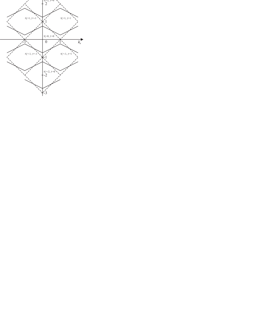
Figure 3: Ground states resonances for a ring with two fermionic species $b=R,L$: Along the lines the energies are degenerate and transport is there maximal. Continuous lines correspond to the interaction parameter $\tilde{W}=2$, dotted lines to the non-interacting case, $\tilde{W}=1$.

Figure 4 shows the ground state energies $E(k_{\mu_{g}},\mathcal{N},\mathcal{J})$ for $k_{\phi}=0$.

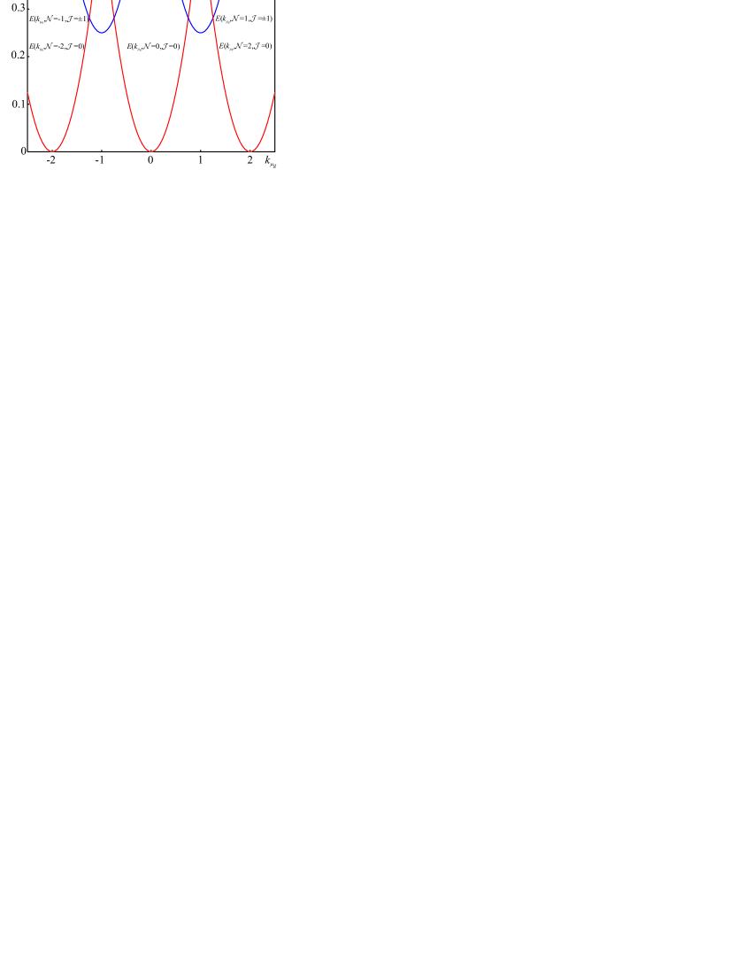
Figure 4: Ground state energies $E(k_{\mu_{g}},\mathcal{N},\mathcal{J})$ for $k_{\phi}=0$ and interaction parameter $\tilde{W}=2$. Notice that the parabolas corresponding to an odd electron number are doubly degenerate.

For values of $k_{\mu_{g}}$ around zero the ring is in the state $(\mathcal{N}=0,\mathcal{J}=0)$. Raising the external gate voltage above $k_{\mu_{g}}=0.75$ leads to a transition to a charged state with one electron. Above $k_{\mu_{g}}=1.25$ the state $(\mathcal{N}=2,\mathcal{J}=0)$ is the one with the lowest energy. We observe that along $k_{\phi}=0$ for the states with an odd number of electrons there is also a degeneracy between the states with the same charge but different current directions.

VI.1.2 SWNT ring

Let us now turn back to the SWNT ring. Due to the presence of the spin and orbital degrees of freedom, the fermionic part of the Hamiltonian is quadratic in all of the variables ${\cal N}_{\tilde{F}j}$ and ${\cal J}_{\tilde{F}j}$, cf. (23). However, it remains gapped only with respect to the total charge and current operators. Let us then introduce for given $\mu_{g}$ and $\tilde{\phi}$ the integer numbers $N_{c}$ and $J_{c}$ which minimize $E_{\rm ring,f}$. Outside resonance, only one couple $(N_{c},J_{c})$ contributes to the grandcanonical sum in (V.4). Nearby resonance we have to include states which differ by one electron and with corresponding current configurations differing by plus/minus one. Moreover, in the low temperature regime $k_{B}T<\varepsilon_{0}$ the quadratic forms in $\hat{H}_{\rm ring,f}$ impose that we only have to take into account those configurations $\{\vec{N}\}$, where the number of electrons in each configuration $(F^{\prime}b^{\prime}\sigma^{\prime})$ differs at most by one (i.e., we neglect ”fermionic excitations”). From now on we measure the number of excess electrons or holes from the charge neutrality point where ${\vec{N}}=0$. Thus, ${N}_{F^{\prime}b^{\prime}\sigma^{\prime}}$ can only assume the values $m$ and $m+1$, where $m\geq 0$ above and $m<0$ below the charge neutrality point. This means that $N_{c}$, obtained by summing over the occupation of all the branches $(F^{\prime}b^{\prime}\sigma^{\prime})$, can be written as $N_{c}=8m+l,\quad m\in Z,\quad l=0,1,\ldots 7.$ Notice that this implies an eight-electron periodicity as a function of the gate voltage. In contrast, as $J_{c}$ counts the occupation difference between the orbital branches, $b=R,L$, it can only take values between $-4$ and $+4$. We can thus simplify the trace operation considerably by summing only over the dominant configurations in (V.4). These are the configurations where $N_{c}\to N_{c}+1$ with ${N}_{Fb\sigma}=m$, and $N_{c}+1\to N_{c}$ with ${N}_{Fb\sigma}=m+1$. We obtain

$$G^{\rm ret}_{Fb\sigma}(\omega,x^{\prime}-x)=\left[1-z\left(\alpha+\frac{1}{q_{c}},0\right)\right]^{C^{2}_{\oplus cq_{0}}}$$ (66)

$$\times \frac{e^{-\beta E^{\phantom{\dagger}}_{\mathrm{ring,f}}(\vec{N}|_{N_{c}+1}}+e^{-\beta E^{\phantom{\dagger}}_{\mathrm{ring,f}}(\vec{N}|_{N_{c}+1})}e^{-i\frac{2\pi}{L}{\rm sgn}(b)(x^{\prime}-x)}}{e^{-\beta E^{\phantom{\dagger}}_{\mathrm{ring,f}}(\vec{N}|_{N_{c}})}+e^{-\beta E^{\phantom{\dagger}}_{\mathrm{ring,f}}(\vec{N}|_{N_{c}+1})}}$$

$$\times \frac{e^{-i\frac{2\pi}{L}(m{\rm sgn}(b)+\tilde{\phi})(x^{\prime}-x)}}{\hbar\omega-{\cal E}_{00}(m+1,N_{c}+1,\mu_{g},\tilde{\phi})+i\eta}.$$

Recalling that $E^{\phantom{\dagger}}_{\mathrm{ring,f}}(\vec{N}|_{N_{c}+1})-E^{\phantom{\dagger}}_{\mathrm{ring,f}}(\vec{N}|_{N_{c}+1})={\cal E}_{00}(m+1,N_{c}+1,\mu_{g},\tilde{\phi})\equiv{\cal E}_{0}$, we obtain

$$|G^{\rm ret}_{Fb\sigma}(\omega,x^{\prime}-x)|^{2}=\left[1-z\left(\alpha+\frac{1}{q_{c}},0\right)\right]^{2C^{2}_{\oplus cq_{0}}}$$ (67)

$$\times \frac{\cos^{2}(\Delta x)+\sin^{2}(\Delta x)\tanh^{2}\Bigl{(}\frac{\beta{\cal E}_{0}}{2}\Bigr{)}}{|\hbar\omega-{\cal E}_{00}(m+1,N_{c}+1,\mu_{g},\tilde{\phi})+i\eta|^{2}},$$

where $\Delta x:=\frac{\pi}{L}(m{\rm sgn}(b)(x^{\prime}-x)$. When Eq. (67) is inserted in Eq. (IV.1) the conductance diverges, as a consequence of the presence of the infinitesimal convergence factor $i\eta$ rather than of a finite line-width Kinaret98 ; Rollb hler99 . Nevertheless, Eq. (67) allows already to discuss the main qualitative features of the conductance, namely the resonance pattern as a function of the applied gate voltage and magnetic field.

To be definite, conductance resonances occur at a degeneracy for the removal of either a counter-clockwise or a clockwise propagating electron. Moreover, as in the spinless case, double resonances occur for special values of the applied magnetic flux and gate voltage, such that clockwise and anti-clockwise propagating modes are simultaneously at resonance. As the ring energy is independent of the spin and Fermi number degrees of freedom, a double resonance is uniquely fixed by $N_{c}$, $J_{c}$. Let us consider e.g. $N_{c}=0$, $J_{c}=0$ and $N_{c}+1=1$, $J_{c}\pm 1$. Then it only exists a configuration with $N_{c}=0$, while there are four equivalent configurations with $N_{c}=+1$, $J_{c}=1$ and four with $N_{c}=1$, $J_{c}=-1$ contributing to the double resonance.

The resonant pattern is easily obtained by approximating the derivative of the Fermi function in Eq. (IV.1) with a delta function Kinaret98 such that $G\propto\sum_{Fb\sigma}|G^{\rm ret}_{Fb\sigma}(0,x^{\prime}-x)|^{2}$, and then evaluating the poles of (67) as a function of $k_{\mu_{g}}$ and $k_{\phi}$. Upon recalling that $N_{c}=8m+l$, with $m\in Z$ and $l=0,1,..7$, we find

$$k_{\mu_{g}}=8m+\frac{4}{\tilde{W}}\Bigl{(}1+\frac{W_{00}}{\varepsilon_{0}}\Bigr{)}+\frac{8W_{00}}{\varepsilon_{0}\tilde{W}}l-\frac{k_{\phi}}{\tilde{W}}{\rm sgn}(b)\;.$$ (68)

Notice that this implies a distance between adjacent resonant lines, with $l$ and $l+1$, of $\Delta k_{\mu_{g}}=\frac{8W_{00}}{\varepsilon_{0}\tilde{W}}$. The corresponding results are shown in figure 5.

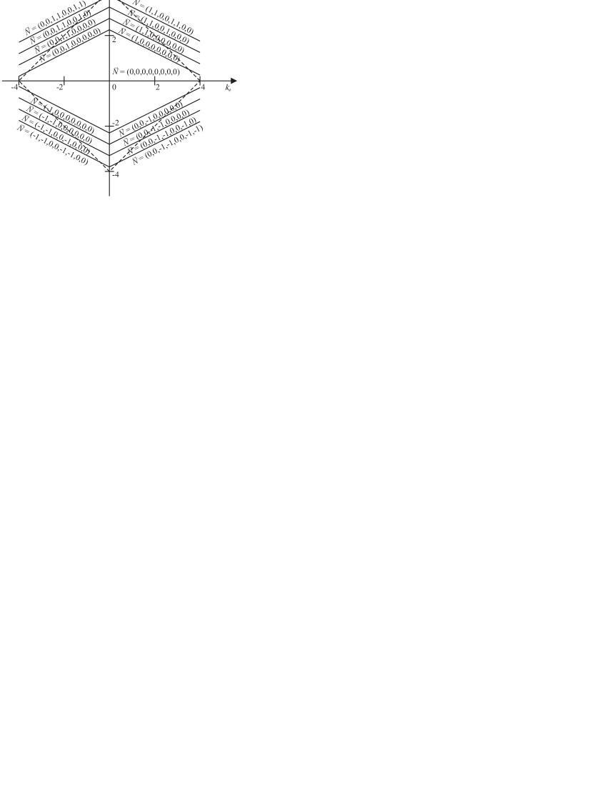
Figure 5: Conductance resonances of the carbon nanotube ring as a function of $k_{\mu_{g}}$ and $k_{\phi}$. The interaction is chosen to be $\tilde{W}=2$. The lines with different slopes correspond to an excess of electrons propagating in opposite directions (counterclockwise and clockwise). Dashed lines are for the non interacting case.

We choose a value of $\tilde{W}=2$ for the plot. The solutions for the non-interacting system are shown with dotted lines. In the non-interacting case the ring is occupied by a multiple of four electrons. From one square to the next other four electrons can be accomodated at one time, as there is no charging energy. In the presence of interactions, however, the picture is entirely different. The former squares are deformed to hexagons which only touch at their vertical boundary. There, the two ground states are degenerate. The conductance is zero here. In the parallel stripes in figure 5 we indicated one possible fermionic configuration only. There is no difference in the energy if we add the first electron to a spin-down state instead of a spin-up one as we did. The choice of $F$ is arbitrary as well. The main difference to the non-interacting case is that, similar to the spinless case, for certain values of $k_{\mu_{g}}$ no conductance resonances can be achieved.

Finally, Eq. (67) predicts a periodic pattern of the conductance as a function of the distance between left and right leads, with maxima when the distance between leads is $x_{R}-x_{L}=L/2$, cf. Fig. 1.

VII Conclusions

In this work the linear conductance of an interacting toroidal SWNT weakly coupled to leads and pierced by a magnetic field has been analyzed. We focussed on low temperatures $k_{B}T<\varepsilon_{0}$, where $\varepsilon_{0}$ is the mean level spacing. In this regime Coulomb blockade effects are known to crucially affect the conductance of a straight SWNT as a function of an applied gate voltage Sapmaz05 ; Moriyama05 . Likewise Coulomb interactions strongly influence the conductance characteristics of the ring. Due to charging effects, the electrons can enter the ring only one by one and not up to four at the time as in the non-interacting case. While in straight tubes the conductance pattern has a four-electron periodicity, for toroidal SWNTs we predict a periodicity of eight electrons. The conductance exhibits Coulomb resonances, and the resonance pattern is a function of the applied magnetic field $\phi$ and gate voltage $\mu_{g}$. In contrast to the non-interacting case, where the parameters $\phi$ and ${\mu_{g}}$ can always be tuned to match a resonance condition, in the interacting system this is no longer possible and we find that at certain values of $\mu_{g}$ a window opens where no conductance resonances can be obtained. Interference effects are manifested in the occurrence of double resonances where electron trajectories propagating clockwise and anticlockwise are degenerate. Finally, the conductance as a function of the distance between left and right leads is maximal when the distance between leads is half of the circumference length, i.e., when clockwise and anti-clockwise propagating electrons have to cover the same source to drain distance.

The conductance of toroidal SWTNs has already been measured in the experiments Shea00 , though not in the Coulomb blockade regime. Thus, we believe that the possible verification of our predictions is within the reach of present experiments.

Appendix A Bogoliubov transformation

The non-diagonal part of (LABEL:V_boson_sc) is given by

$$\hat{H}_{\mathrm{nd}}=\varepsilon_{0}\sum_{q\neq 0}|n_{q}|b_{\oplus cq}^{\dagger}b_{\oplus cq}+\frac{1}{2}\sum_{q\neq 0}4|n_{q}|W_{q,-q}\times$$

$$\times \Bigl{(}b_{\oplus cq}b_{\oplus c-q}+b_{\oplus cq}b^{\dagger}_{\oplus cq}+b^{\dagger}_{\oplus c-q}b_{\oplus c-q}+b^{\dagger}_{\oplus c-q}b^{\dagger}_{\oplus cq}\Bigr{)}.$$

The goal of the Bogoliubov transformation is the derivation of new operators, in terms of which $\hat{H}_{\mathrm{nd}}$ is diagonal. In general, we can write them as a linear combination of the old bosonic operators $b^{\dagger}_{\oplus cq}$ and $b_{\oplus cq}$:

$$a^{\dagger}_{\oplus cq} = \sum_{q^{\prime}}(U_{qq^{\prime}}b^{\dagger}_{\oplus cq^{\prime}}-V_{qq^{\prime}}b_{\oplus cq^{\prime}}),$$ (70)

$$a_{\oplus cq} = \sum_{q^{\prime}}(-V_{qq^{\prime}}b^{\dagger}_{\oplus cq^{\prime}}+U_{qq^{\prime}}b_{\oplus cq^{\prime}}).$$ (71)

Of course, these operators have to fulfill the bosonic commutation relations:

$$[a_{\oplus cq},a^{\dagger}_{\oplus cq^{\prime}}] = \delta_{qq^{\prime}},$$ (72)

$$\left[a_{\oplus cq},a_{\oplus cq^{\prime}}\right] = [a^{\dagger}_{\oplus cq},a^{\dagger}_{\oplus cq^{\prime}}]=0.$$ (73)

Additionally, in order to ensure the diagonal form of $\hat{H}_{\mathrm{nd}}$ in terms of the new operators, the conditions

$$[\hat{H}_{c},a^{\dagger}_{\oplus cq}]=\varepsilon_{cq}a^{\dagger}_{\oplus cq} \Longleftrightarrow [\hat{H}_{c},a_{\oplus cq}]=-\varepsilon_{cq}a_{\oplus cq}\quad$$ (74)

have to be fulfilled. Note that also new energies $\varepsilon_{cq}$ have been introduced. The calculation of the transformation matrices $U$ and $V$ follows closely the guidelines in Avery76 . The result is

$$U = \frac{1}{2}\left(\begin{array}[]{cc}\sqrt{\frac{\varepsilon_{cq}}{2\varepsilon_{0q}}}+\sqrt{\frac{\varepsilon_{0q}}{2\varepsilon_{cq}}}&\quad-\sqrt{\frac{\varepsilon_{cq}}{2\varepsilon_{0q}}}-\sqrt{\frac{\varepsilon_{0q}}{2\varepsilon_{cq}}}\\ \sqrt{\frac{\varepsilon_{cq}}{2\varepsilon_{0q}}}+\sqrt{\frac{\varepsilon_{0q}}{2\varepsilon_{cq}}}&\quad\sqrt{\frac{\varepsilon_{cq}}{2\varepsilon_{0q}}}+\sqrt{\frac{\varepsilon_{0q}}{2\varepsilon_{cq}}}\end{array}\right)$$ (77)

$$V = \frac{1}{2}\left(\begin{array}[]{cc}\sqrt{\frac{\varepsilon_{cq}}{2\varepsilon_{0q}}}-\sqrt{\frac{\varepsilon_{0q}}{2\varepsilon_{cq}}}&\quad-\sqrt{\frac{\varepsilon_{cq}}{2\varepsilon_{0q}}}+\sqrt{\frac{\varepsilon_{0q}}{2\varepsilon_{cq}}}\\ -\sqrt{\frac{\varepsilon_{cq}}{2\varepsilon_{0q}}}+\sqrt{\frac{\varepsilon_{0q}}{2\varepsilon_{cq}}}&\quad-\sqrt{\frac{\varepsilon_{cq}}{2\varepsilon_{0q}}}+\sqrt{\frac{\varepsilon_{0q}}{2\varepsilon_{cq}}}\end{array}\right),$$ (80)

where $\varepsilon_{0q}=\varepsilon_{0}|n_{q}|$ and the transformed energies $\varepsilon_{cq}$ are given by

$$\varepsilon_{cq}=\varepsilon_{0q}\sqrt{1+8W_{q,-q}/\varepsilon_{0}}.$$ (82)

Using the abbreviations $\alpha_{q}=\frac{1}{2}\sqrt{\frac{\varepsilon_{0q}}{2\varepsilon_{cq}}}$ and $\beta_{q}=\frac{1}{2}\sqrt{\frac{\varepsilon_{cq}}{2\varepsilon_{0q}}}$ the new operators read, assuming $q>0$:

$$a^{\dagger}_{\oplus cq} = (\alpha_{q}+\beta_{q})(b^{\dagger}_{\oplus c-q}+b^{\dagger}_{\oplus cq})$$

$$+ (\beta_{q}-\alpha_{q})(b_{\oplus c-q}+b_{\oplus cq}),$$

$$a_{\oplus cq} = (\beta_{q}-\alpha_{q})(b^{\dagger}_{\oplus c-q}+b^{\dagger}_{\oplus cq})$$

$$+ (\alpha_{q}+\beta_{q})(b_{\oplus c-q}+b_{\oplus cq}),$$

$$a^{\dagger}_{\oplus c-q} = (\alpha_{q}+\beta_{q})(b^{\dagger}_{\oplus c-q}-b^{\dagger}_{\oplus cq})$$

$$+ (\alpha_{q}-\beta_{q})(b_{\oplus c-q}-b_{\oplus cq}),$$

$$a_{\oplus c-q} = (\alpha_{q}-\beta_{q})(b^{\dagger}_{\oplus c-q}-b^{\dagger}_{\oplus cq})$$

$$+ (\alpha_{q}+\beta_{q})(b_{\oplus c-q}-b_{\oplus cq}).$$

The inverse of the transformation is

$$b^{\dagger}_{\oplus cq} = \frac{-(\alpha_{q}+\beta_{q})(a^{\dagger}_{\oplus c-q}-a^{\dagger}_{\oplus cq})}{8\alpha_{q}\beta_{q}}$$

$$+ \frac{(\alpha_{q}-\beta_{q})(a_{\oplus c-q}+a_{\oplus cq})}{8\alpha_{q}\beta_{q}},$$

$$b_{\oplus cq} = \frac{(\alpha_{q}-\beta_{q})(a^{\dagger}_{\oplus c-q}+a^{\dagger}_{\oplus cq})}{8\alpha_{q}\beta_{q}}$$

$$+ \frac{-(\alpha_{q}+\beta_{q})(a_{\oplus c-q}-a_{\oplus cq})}{8\alpha_{q}\beta_{q}},$$

$$b^{\dagger}_{\oplus c-q} = \frac{(\alpha_{q}+\beta_{q})(a^{\dagger}_{\oplus c-q}+a^{\dagger}_{\oplus cq})}{8\alpha_{q}\beta_{q}}$$

$$+ \frac{-(\alpha_{q}-\beta_{q})(a_{\oplus c-q}-a_{\oplus cq})}{8\alpha_{q}\beta_{q}},$$

$$b_{\oplus c-q} = \frac{-(\alpha_{q}-\beta_{q})(a^{\dagger}_{\oplus c-q}-a^{\dagger}_{\oplus cq})}{8\alpha_{q}\beta_{q}}$$

$$+ \frac{(\alpha_{q}+\beta_{q})(a_{\oplus c-q}+a_{\oplus cq})}{8\alpha_{q}\beta_{q}}.$$

The inverse transformation can also be written in a more concise way:

$$b_{\tilde{F}jq}=\sum_{q^{\prime}}\left(S_{\tilde{F}jqq^{\prime}}a_{\tilde{F}jq^{\prime}}+C_{\tilde{F}jqq^{\prime}}a_{\tilde{F}jq}^{\dagger}\right),$$

where we have for the spin related coefficients $S$ and $C$:

$$S_{\oplus sqq^{\prime}} = S_{\ominus sqq^{\prime}}=S_{\ominus cqq^{\prime}}=\delta_{qq^{\prime}},$$

$$C_{\oplus sqq^{\prime}} = C_{\ominus sqq^{\prime}}=C_{\ominus cqq^{\prime}}=0,$$

while for the charge related ones, we have to take care of the sign of $q$. Let us choose $q>0$:

$$S_{\oplus cqq^{\prime}} = \delta_{qq^{\prime}}\frac{\alpha_{q}+\beta_{q}}{8\alpha_{q}\beta_{q}}-\delta_{q-q^{\prime}}\frac{\alpha_{q}+\beta_{q}}{8\alpha_{q}\beta_{q}},$$

$$C_{\oplus cqq^{\prime}} = \delta_{qq^{\prime}}\frac{\alpha_{q}-\beta_{q}}{8\alpha_{q}\beta_{q}}+\delta_{q-q^{\prime}}\frac{\alpha_{q}-\beta_{q}}{8\alpha_{q}\beta_{q}},$$

$$S_{\oplus c-qq^{\prime}} = \delta_{qq^{\prime}}\frac{\alpha_{q}+\beta_{q}}{8\alpha_{q}\beta_{q}}+\delta_{q-q^{\prime}}\frac{\alpha_{q}+\beta_{q}}{8\alpha_{q}\beta_{q}},$$

$$C_{\oplus c-qq^{\prime}} = \delta_{qq^{\prime}}\frac{\alpha_{q}-\beta_{q}}{8\alpha_{q}\beta_{q}}-\delta_{q-q^{\prime}}\frac{\alpha_{q}-\beta_{q}}{8\alpha_{q}\beta_{q}}.$$

The final result for the diagonalised Hamiltonian is then

$$\hat{H}_{\mathrm{ring}} = \sum_{\tilde{F}j}\sum_{q\neq 0}\varepsilon_{\tilde{F}jq}a_{\tilde{F}jq}^{\dagger}a^{\phantom{\dagger}}_{\tilde{F}jq}+\varepsilon_{0}\sum_{Fr\sigma}\frac{\mathcal{N}^{2}_{Fr\sigma}}{2}+$$ (83)

$$+ \varepsilon_{0}\tilde{\phi}\sum_{Fr\sigma}\mbox{sgn}(r)\mathcal{N}_{Fr\sigma}+\frac{1}{2}W_{00}\mathcal{N}^{2},$$

where we introduced the energies

$$\varepsilon_{\oplus sq}=\varepsilon_{\ominus sq}=\varepsilon_{\ominus cq}=\varepsilon_{0q}\mbox{ and }\varepsilon_{\oplus cq}=\varepsilon_{cq}.$$ (84)

Appendix B The bosonic correlator

We evaluate in this appendix explicitly the bosonic part of the Green’s function, Eq. (V.3), in the so called Luttinger limit, where i) we assume a linear dispersion: $\varepsilon_{cq}=\varepsilon_{0q}/K_{c}$, with coupling constant $K_{c}=\sqrt{1+8W_{q_{0}-q_{0}}/\varepsilon_{0}}$; ii) we assume an exponential decay of the parameter $C_{\oplus cqq}$ entering the Bogoliubov transformation: $C^{2}_{\oplus cqq}=C^{2}_{\oplus cq_{0}}e^{-q/q_{c}}$, with $q_{c}$ a momentum cut-off. Let us then start from Eq. (V.3):

$$\left\langle\psi^{\dagger}_{Fb\sigma}(x^{\prime},-t)\psi^{\phantom{\dagger}}_{Fb\sigma}(x,0)\right\rangle_{b}=\frac{1}{1-e^{-\alpha\frac{2\pi}{L}}}$$

$$\times \exp\left\{-\frac{1}{4}\sum_{q>0}\frac{e^{-\alpha q}}{n_{q}}\right.\left[\sum_{\tilde{F}j}Q_{\tilde{F}jq}(t,{\rm sgn}(b)(x^{\prime}-x))\right.$$

$$+ \left.2C^{2}_{\oplus cqq}[Q_{cq}(t,(x^{\prime}-x))+Q_{cq}(t,-(x^{\prime}-x))]\right]\left.\right\},$$

where we introduced the correlation function

$$Q_{\gamma q}(t,x) := i\sin\Bigl{(}\frac{\varepsilon_{\gamma q}t}{\hbar}-qx\Bigr{)}$$

$$+ \left[1-\cos\Bigl{(}\frac{\varepsilon_{\gamma q}t}{\hbar}-qx\Bigr{)}\right]\coth\Bigl{(}\frac{\beta\varepsilon_{\gamma q}}{2}\Bigr{)}.$$

In the low temperature regime we can approximate $\coth(\beta\varepsilon_{0q}/2)$ and $\coth(\beta\varepsilon_{cq}/2)$ by 1. We perform now the Luttinger approximation and recall that $q=2n\pi/L$. Rewriting the sin and cos functions as exponentials and remembering the formula

$$\sum_{n>0}\frac{e^{an}}{n}=-\ln(1-e^{a}),\quad|e^{a}|<1,$$ (87)

we arrive at

$$\left\langle\psi^{\dagger}_{Fb\sigma}(x^{\prime},-t)\psi^{\phantom{\dagger}}_{Fb\sigma}(x,0)\right\rangle_{b}$$ (88)

$$= \left[1-z\Bigl{(}\alpha+\frac{1}{q_{c}},0\Bigr{)}\right]^{C^{2}_{\oplus cq_{0}}}$$

$$\times \left[1-z\Bigl{(}\alpha,v_{F}t+{\rm sgn}(b)(x^{\prime}-x)\Bigr{)}\right]^{-3/4}$$

$$\times \left[1-z\Bigl{(}\alpha,{\rm v}_{c}t+{\rm sgn}(b)(x^{\prime}-x)\Bigr{)}\right]^{-1/4}$$

$$\times \left[1-z\Bigl{(}\alpha+\frac{1}{q_{c}},{\rm v}_{c}t+(x^{\prime}-x)\Bigr{)}\right]^{-\frac{1}{2}C^{2}_{\oplus cq_{0}}}$$

$$\times \left[1-z\Bigl{(}\alpha+\frac{1}{q_{c}},{\rm v}_{c}t-(x^{\prime}-x)\Bigr{)}\right]^{-\frac{1}{2}C^{2}_{\oplus cq_{0}}},$$

where we have defined the function

$$z(\alpha,x):=e^{(-\alpha+ix)\frac{2\pi}{L}}.$$ (89)

Because the functions entering (88) are periodic in time, we can write the bosonic correlation function as a product of Fourier series. To this extent we use the relation

$$(1-z)^{\gamma}=\sum_{k=0}^{\infty}\frac{\Gamma(k-\gamma)}{k!\Gamma(-\gamma)}z^{k},\quad|z|<1,$$ (90)

which yields the final result

$$\left\langle\psi^{\dagger}_{Fb\sigma}(x^{\prime},-t)\psi_{Fb\sigma}(x,0)\right\rangle_{b}=\left[1-z\left(\alpha+\frac{1}{q_{c}},0\right)\right]^{C^{2}_{\oplus cq_{0}}}$$ (91)

$$\times \sum_{k=0}^{\infty}r_{k}\Biggl{(}\alpha,-\frac{3}{4},\mbox{sgn}(b)(x^{\prime}-x)\Biggr{)}e^{\frac{i}{\hbar}\varepsilon_{0}kt}$$

$$\times \sum_{l=0}^{\infty}s_{l}(b,x^{\prime}-x)e^{\frac{i}{\hbar}\varepsilon_{c}lt}.$$

Here we have defined

$$r_{k}(\alpha,\gamma,x):=\frac{\Gamma(k-\gamma)}{k!\Gamma(-\gamma)}e^{k\frac{2\pi}{L}(-\alpha+ix)},$$

$$s_{l}(b,x^{\prime}-x) := \phantom{\times}\sum_{n_{1}=0}^{l}r_{n_{1}}\Biggl{(}\alpha,-\frac{1}{4},\mbox{sgn}(b)(x^{\prime}-x)\Biggr{)}$$

$$\times\sum_{n_{2}=0}^{l-n_{1}}r_{n_{2}}\left(\alpha+\frac{1}{q_{c}},-\frac{1}{2}C^{2}_{\oplus cq_{0}},(x^{\prime}-x)\right)$$

$$\times\sum_{n_{3}=0}^{l-n_{1}-n_{2}}r_{n_{3}}\left(\alpha+\frac{1}{q_{c}},-\frac{1}{2}C^{2}_{\oplus cq_{0}},-(x^{\prime}-x)\right),$$

where $\Gamma$ is the gamma function.

References

- (1) Y. Aharonov and D. Bohm, Phys. Rev. 115, 485 (1959).
- (2) B. L. Al’tschuler, A. G. Aronov and B. Z. Spivak, Pis’ma Zh.Eksp. Teor. Fiz. 33, 101 (1981) [JETP Lett. 33, 94 (1981)].
- (3) E. A. Jagla and C. A. Balseiro, Phys. Rev. Lett. 68, 1220 (1992).
- (4) J. M. Kinaret, M. Jonson and R. I. Shekhter, Phys. Rev. B 57, 3777 (1998).
- (5) M. Pletyukhov, V. Gritsev and N. Pauget, Phys. Rev. B 74, 045301 (2006).
- (6) R. Saito, G. Dresselhaus and M. Dresselhaus, Physical Properties of Carbon Nanotubes (Imperial College Press, London, 1998).
- (7) R. Egger and A. O. Gogolin, Phys. Rev. Lett. 79, 5082 (1997); Eur. Phys. J. B 3, 281 (1998).
- (8) C. Kane, L. Balents and M. P. A. Fisher, Phys. Rev. Lett. 79, 5086 (1997).
- (9) S. J. Tans et al., Nature (London) 386, 474 (1997).
- (10) M. Bockrath et al., Nature (London) 397, 598 (1999).
- (11) H. W. Ch. Postma et al., Science 293, 76 (2001).
- (12) J. Lee et al., Phys. Rev. Lett. 93, 166403 (2004).
- (13) D. H. Cobden and J. Nygård, Phys. Rev. Lett. 89, 046803 (2002).
- (14) W. Liang, M. Bockrath and H. Park, Phys. Rev. Lett. 88, 126801 (2002).
- (15) S. Sapmaz, P. Jarillo-Herrero, J. Kong, C. Dekker, L. P. Kouwenhoven and H. S. J. van der Zant, Phys. Rev. B 71, 153402 (2005).
- (16) S. Moriyama, T. Fuse, M. Suzuki, Y. A. Yagi and K. Ishibashi, Phys. Rev. Lett. 94, 186806 (2005).
- (17) F. Kuemmeth, S. Ilani, D. C. Ralph and P. L. McEuen, Nature 452, 448 (2008).
- (18) Y. Oreg, K. Byczuk and B. I. Halperin, Phys. Rev. Lett. 85, 365 (2000).
- (19) L. Mayrhofer and M. Grifoni, Phys. Rev. B 74, 121403R (2006); Europ. Phys. J. B 56, 107 (2007).
- (20) L. Mayrhofer and M. Grifoni, Eur. Phys. J. B in press and arXiv:0804.3360.
- (21) J. Liu et al., Nature 385, 780 (1997).
- (22) R. Martel, H. R. Shea and Ph. Avouris, Nature 398, 299 (1999).
- (23) H. R. Shea, R. Martel and Ph. Avouris, Phys. Rev. Lett. 84, 4441(2000).
- (24) M. F. Lin and D. S. Chuu, Phys. Rev. B 57, 6731 (1998).
- (25) A. A. Odintsov, W. Smit and H. Yoshioka, Europhysics Lett. 45, 598 (1999).
- (26) J. Rollbühler and A. A. Odintsov, Physica B 280, 386 (1999).
- (27) S. Latil, S. Roche and A. Rubio, Phys. Rev. B 67, 165420 (2003).
- (28) G. C. Rocha, M. Pacheco, Z. Particevic and A. Latgeé, Phys. Rev. B 70, 233402 (2004).
- (29) H.-K. Zhao and J. Wang, Phys. Lett. A 325, 407 (2004).
- (30) M. Jack and M. Encinosa, arXiv:0709.0760v1
- (31) J. van Delft and H. Schoeller, Ann. Phys. 7, 225 (1998).
- (32) D. Loss, Phys. Rev. Lett. 69, 343 (1992).
- (33) J. Avery, Creation and Annihilation Operators (McGraw-Hill, New York 1976).