Linear sigma model at finite density in the $1/N$ expansion to next-to-leading order

Abstract

We study relativistic Bose–Einstein condensation at finite density and temperature using the linear sigma model in the one-particle-irreducible $1/N$-expansion. We derive the effective potential to next-to-leading (NLO) order and show that it can be renormalized in a temperature-independent manner. As a particular application, we study the thermodynamics of the pion gas in the chiral limit as well as with explicit symmetry breaking. At nonzero temperature we solve the NLO gap equation and show that the results describe the chiral-symmetry-restoring second-order phase transition in agreement with general universality arguments. However, due to nontrivial regularization issues, we are not able to extend the NLO analysis to nonzero chemical potential.

I Introduction

The Lagrangian of quantum chromodynamics (QCD) with $N_{f}$ quark flavors has an extended $\mathrm{SU}(N_{f})_{L}\times\mathrm{SU}(N_{f})_{R}$ symmetry in the chiral limit, which is not respected by the true QCD ground state. The chiral symmetry is spontaneously broken down to the vector subgroup $\mathrm{SU}(N_{f})_{V}$ by quantum effects, and according to Goldstone’s theorem there are $N_{f}^{2}-1$ massless excitations associated with this breaking. For $N_{f}=2$, this implies the existence of three Goldstone bosons, which are identified with the pions. The fact that these particles are not exactly massless is taken into account by small nonzero quark masses in the QCD Lagrangian. In low-energy QCD phenomenology, one takes advantage of the isomorphism between the groups $\mathrm{SU}(2)\times\mathrm{SU}(2)$ and $\mathrm{SO}(4)$ to describe the pions as well as the sigma by scalar field theory with this symmetry. At low temperature, the $\mathrm{O}(4)$ symmetry is broken down to $\mathrm{O}(3)$ either explicitly or spontaneously. In the latter case, one expects it to be restored at sufficiently high temperature. Lattice simulations of QCD suggest that the critical temperature is around $170\text{ MeV}$, depending on the masses of the quarks.

At zero temperature, the $\mathrm{O}(N)$ linear sigma model was studied a long time ago using the one-particle-irreducible (1PI) $1/N$-expansion, to leading order (LO) by Coleman et al. Coleman et al. (1974), and to next-to-leading order (NLO) by Root Root (1974). At finite temperature but vanishing chemical potential, the LO thermodynamics was studied by Meyer-Ortmanns et al. Meyer-Ortmanns et al. (1993). Later several attempts to calculate the pressure to next-to-leading order have been made, but the approximations made were uncontrolled and renormalization was ignored. Due to the nontrivial renormalization issues, the NLO pressure was calculated only recently Andersen et al. (2004). Specifically, one problem was that the effective potential seemed to have ultraviolet divergences which were temperature-dependent, except at its minimum. Renormalization of the effective potential could therefore be carried out with temperature-independent counterterms only on shell.

Sigma models have also been investigated in detail at finite temperature using other methods: Optimized perturbation theory Chiku and Hatsuda (1998), two-particle-irreducible (2PI) effective action either in the Hartree or large-$N$ approximation Cornwall et al. (1974); Amelino-Camelia and Pi (1993); Amelino-Camelia (1997); Petropoulos (1999); Lenaghan and Rischke (2000). In these calculations, one typically encounters a local gap equation for a mass parameter, which is straightforward to solve. Beyond leading order, the resulting equations are nonlocal and much harder to solve.

Linear sigma models at finite chemical potential that describe relativistic Bose–Einstein condensation, have received interest in recent years due to the possibility of e.g. pion and kaon condensation in compact stars Kaplan and Reddy (2002); Bedaque and Schaefer (2002). Pion condensation and the phase diagram of two-flavor QCD have been investigated using chiral perturbation theory  Son and Stephanov (2001); Splittorff et al. (2001); Kogut and Toublan (2001); Loewe and Villavicencio (2003, 2004, 2005), lattice QCD Kogut and Sinclair (2002); Gupta (2002), ladder QCD Barducci et al. (2003), chiral quark model Jakovac et al. (2004), Nambu–Jona-Lasinio models in the mean-field approximation Nambu and Jona-Lasinio (1961); Hufner et al. (1994); Zhuang et al. (1994); Barducci et al. (2004); He et al. (2005); Ebert and Klimenko (2006a, b); Andersen and Kyllingstad (2007), and the linear sigma model using the Hartree approximation Mao et al. (2006), or the large-$N$ approximation Andersen (2007).

In the present paper, we extend the calculation of Ref. Andersen et al. (2004) using the 1PI-$1/N$ expansion by including nonzero chemical potential. In contrast to the previous work we show that, when interpreted properly, the effective potential can be renormalized in a temperature-independent manner even off its minimum. We apply the method to the study of pion condensation. The paper is organized as follows. In Sec. II, we introduce the general model and briefly discuss interacting bosons at finite temperature and density. In Sec. III, we review the standard calculation of the LO effective potential and determine the phase diagram. In Sec. IV, we calculate the NLO effective potential and discuss in detail its renormalization. In particular, we demonstrate how it is used to derive a renormalized gap equation. In Sec. V we summarize and conclude.

II Effective action in $1/N$ expansion

II.1 The model

The Euclidean Lagrangian for a Bose gas of $N$ real scalars is given by Andersen et al. (2004)

$$\mathcal{L}=\frac{1}{2}(\partial_{\mu}\phi_{i})^{2}+\frac{\lambda_{b}}{8N}(\phi_{i}\phi_{i}-Nf_{\pi,b}^{2})^{2}-\sqrt{N}H\phi_{N},$$ (1)

where $i=1,\dotsc,N$. The parameters $f_{\pi,b}$ and $\lambda_{b}$ denote the bare pion decay constant and coupling, respectively. If $H=0$, the Lagrangian has an $\mathrm{O}(N)$ symmetry, while if $H\neq 0$, this symmetry is explicitly broken down to $\mathrm{O}(N-1)$. Each generator of the symmetry group gives rise to a conserved charge and for $\mathrm{O}(N)$ there are $N(N-1)/2$ such charges. We can characterize a system described by Eq. (1) by the expectation values of the conserved charges $Q_{i}$ and for each of them we can in principle introduce a chemical potential $\mu_{i}$. Nevertheless, it is only possible to simultaneously specify two different charges if they commute. For the $\mathrm{O}(N)$ symmetry the maximum number of commuting charges is $\lfloor N/2\rfloor$ (here $\lfloor\,\rfloor$ denotes the integer part of a real number) Haber and Weldon (1982).

If we treat two real scalar fields, $\phi_{R}$ and $\phi_{I}$, as the real and imaginary part of a single complex field, $\Phi=(\phi_{R}+i\phi_{I})/\sqrt{2}$, the conserved charge $Q$ can be incorporated by making the substitution in the Euclidean Lagrangian,

$$\begin{split}\partial_{0}\Phi&\to(\partial_{0}-\mu)\Phi,\\ \partial_{0}\Phi^{\dagger}&\to(\partial_{0}+\mu)\Phi^{\dagger}.\end{split}$$ (2)

The actual value of the charge density in thermodynamic equilibrium is then determined from the free energy density ${\cal F}$ as $Q=-{\partial{\cal F}}/{\partial\mu}$.

In order to eliminate the quartic term from the Lagrangian (1), we introduce an auxiliary field $\alpha$ and add to Eq. (1) the following term Coleman et al. (1974),

$$\mathcal{L}_{\alpha}=\frac{N}{2\lambda_{b}}\left[\alpha-\frac{i\lambda_{b}}{2N}(\phi_{i}\phi_{i}-Nf^{2}_{\pi,b})\right]^{2}.$$

The Lagrangian can now be written as

$$\mathcal{L}=\frac{1}{2}(\partial_{\mu}\phi_{i})^{2}-\frac{i}{2}\alpha(\phi_{i}\phi_{i}-Nf_{\pi,b}^{2})+\frac{N}{2\lambda_{b}}\alpha^{2}-\sqrt{N}H\phi_{N}.$$ (3)

By using the equation of motion for $\alpha$, one can eliminate this field altogether and thus recover the original Lagrangian (1).

Another virtue of introducing the auxiliary field is that the Lagrangian now depends linearly on the two parameters, $f^{2}_{\pi,b}$ and $1/\lambda_{b}$. As will be shown later, the divergences that appear in the effective potential may be removed by their suitable redefinition. For the sake of systematic expansion in powers of $1/N$, we write them as

$$\begin{split}f_{\pi,b}^{2}&=f_{\pi}^{2}+a_{0}+\frac{1}{N}a_{1}+\dotsb,\\ \frac{1}{\lambda_{b}}&=\frac{1}{\lambda}+b_{0}+\frac{1}{N}b_{1}+\dotsb,\end{split}$$ (4)

where $f_{\pi}$ and $\lambda$ are the renormalized decay constant and coupling. The parameters $a_{0,1}$ and $b_{0,1}$ are the counterterms needed to cancel the divergences at the corresponding orders in $1/N$.

II.2 Application to pion gas

We next use our model to describe the pion gas at finite temperature and chemical potential. The vacuum expectation value $\phi_{0}$ of $\phi_{N}$ is interpreted as the usual chiral condensate. Using Eq. (2) we introduce isospin chemical potential $\mu_{I}$ for the pair $\phi_{1},\phi_{2}$, which are hence identified with the real and imaginary parts of the charged pion field. The neutral pion is $\phi_{3}$. The Lagrangian (3) thus becomes

$$\mathcal{L}=\frac{1}{2}(\partial_{\mu}\phi_{i})^{2}-\frac{i}{2}\alpha(\phi_{i}\phi_{i}-Nf_{\pi,b}^{2})+\frac{N}{2\lambda_{b}}\alpha^{2}-\sqrt{N}H\phi_{N}\\ -i\mu_{I}(\phi_{1}\partial_{0}\phi_{2}-\phi_{2}\partial_{0}\phi_{1})-\frac{1}{2}\mu_{I}^{2}(\phi_{1}^{2}+\phi_{2}^{2}).$$

The Lagrangian is quadratic in the scalar fields $\phi_{i}$ and we next integrate over the $N-3$ fields $\phi_{3},\dotsc,\phi_{N-1}$. This gives an effective action for the remaining fields $\alpha,\phi_{1},\phi_{2},\phi_{N}$,

$$S_{\text{eff}}=\frac{1}{2}(N-3)\operatorname{Tr}\log(-\partial^{2}-i\alpha)+\int_{0}^{\beta}d\tau\int d^{3}x\\ \times\left[\frac{1}{2}(\partial_{\mu}\phi_{1})^{2}+\frac{1}{2}(\partial_{\mu}\phi_{2})^{2}+\frac{1}{2}(\partial_{\mu}\phi_{N})^{2}-\sqrt{N}H\phi_{N}\right.\\ -i\mu_{I}(\phi_{1}\partial_{0}\phi_{2}-\phi_{2}\partial_{0}\phi_{1})-\frac{1}{2}\mu_{I}^{2}(\phi_{1}^{2}+\phi_{2}^{2})\\ \left.+\frac{N}{2\lambda_{b}}\alpha^{2}-\frac{i}{2}\alpha(\phi_{1}^{2}+\phi_{2}^{2}+\phi_{N}^{2}-Nf_{\pi,b}^{2})\right].$$ (5)

Now we introduce a nonzero expectation value $\rho_{0}$ for $\phi_{1}$ to allow for a nonzero pion condensate. We also expand the auxiliary field $\alpha$ around its expectation value $iM^{2}$. Thus we make the following replacements in Eq. (5),

$$\begin{split}\phi_{1}&\to\sqrt{N}\rho_{0}+\phi_{1},\\ \phi_{N}&\to\sqrt{N}\phi_{0}+\phi_{N},\\ \alpha&\to iM^{2}+\frac{\alpha}{\sqrt{N}}.\end{split}$$ (6)

The various factors of $\sqrt{N}$ do not change the physics, but merely facilitate the calculations in powers of $1/N$. Making the substitutions (6) in Eq. (5), the effective action becomes 

$$S_{\text{eff}}=\frac{1}{2}(N-3)\operatorname{Tr}\log\left(-\partial^{2}+M^{2}-\frac{i\alpha}{\sqrt{N}}\right)+\int_{0}^{\beta}d\tau\int d^{3}x\left[\frac{1}{2}(\partial_{\mu}\phi_{1})^{2}+\frac{1}{2}(\partial_{\mu}\phi_{2})^{2}+\frac{1}{2}(\partial_{\mu}\phi_{N})^{2}\right.\\ -NH\phi_{0}-i\mu_{I}(\phi_{1}\partial_{0}\phi_{2}-\phi_{2}\partial_{0}\phi_{1})-\frac{1}{2}\mu_{I}^{2}(N\rho_{0}^{2}+\phi_{1}^{2}+\phi_{2}^{2})-\frac{N}{2\lambda_{b}}M^{4}+\frac{1}{2\lambda_{b}}\alpha^{2}+\frac{1}{2}M^{2}(\phi_{1}^{2}+\phi_{2}^{2}+\phi_{N}^{2})\\ \left.-i\alpha\left(\phi_{0}\phi_{N}+\rho_{0}\phi_{1}+\frac{\phi_{1}^{2}+\phi_{2}^{2}+\phi_{N}^{2}}{2\sqrt{N}}\right)+\frac{1}{2}NM^{2}(\phi_{0}^{2}+\rho_{0}^{2}-f_{\pi,b}^{2})\right].$$ (7)

Expanding Eq. (7) up to second order in $1/\sqrt{N}$ and using Eq. (4), we obtain

$$\frac{S_{\text{eff}}}{\beta V}=\frac{1}{2}NM^{2}(\phi_{0}^{2}+\rho_{0}^{2}-f_{\pi}^{2})-\frac{NM^{4}}{2\lambda}-NH\phi_{0}-\frac{1}{2}N\mu_{I}^{2}\rho_{0}^{2}+\frac{1}{2}(N-3)\hbox{$\sum$}\!\!\!\!\!\!\int_{P}\ln(P^{2}+M^{2})-\frac{1}{2}NM^{2}a_{0}-\frac{1}{2}NM^{4}b_{0}\\ +\frac{1}{2}\hbox{$\sum$}\!\!\!\!\!\!\int_{P}\chi^{T}(-P)\left(\begin{array}[]{cccc}\frac{1}{2}\Pi(P,M)+\frac{1}{\lambda}+b_{0}&-i\phi_{0}&-i\rho_{0}&0\\ -i\phi_{0}&P^{2}+M^{2}&0&0\\ -i\rho_{0}&0&P^{2}+m^{2}&-2\mu_{I}\omega_{n}\\ 0&0&2\mu_{I}\omega_{n}&P^{2}+m^{2}\\ \end{array}\right)\chi(P)-\frac{1}{2}M^{2}a_{1}-\frac{1}{2}M^{4}b_{1},$$ (8)

where $\chi(P)=(\alpha(P),\phi_{N}(P),\phi_{1}(P),\phi_{2}(P))^{T}$ and $m^{2}=M^{2}-\mu_{I}^{2}$. The self-energy function is

$$\Pi(P,M)=\hbox{$\sum$}\!\!\!\!\!\!\int_{Q}\frac{1}{Q^{2}+M^{2}}\frac{1}{(P+Q)^{2}+M^{2}}.$$

We have also introduced the notation

$$\hbox{$\sum$}\!\!\!\!\!\!\int_{P}=T\sum_{\omega_{n}=2\pi nT}\int\frac{d^{3}p}{(2\pi)^{3}}.$$

The sum-integral involves a summation over Matsubara frequencies and an integral over three-momenta $p$. At zero temperature, the sum-integrals reduce to a four-dimensional integral, where we write

$$\int_{P}=\int\frac{d^{4}P}{(2\pi)^{4}}.$$

Such integrals are regularized by a four-dimensional ultraviolet cutoff $\Lambda$.

In deriving Eq. (8) we implicitly assumed that the classical fields $\phi_{0},\rho_{0},M^{2}$ are constant. This makes it possible to define the effective potential by dividing by the space volume and inverse temperature. Specifically, we define its LO and NLO parts by

$$-\frac{S_{\text{eff}}}{\beta V}=NV_{\text{LO}}+V_{\text{NLO}}.$$

In equilibrium, the effective potential is then equal to the pressure.

At this point it is worthwhile to discuss explicitly the symmetries of the model with(out) the $H$ term and the chemical potential, and their spontaneous breaking by the condensates $\phi_{0},\rho_{0}$, in the physical case $N=4$. First, in the chiral limit, $H=0$, the system has $\mathrm{O(4)}$ symmetry in the vacuum which is broken explicitly by the chemical potential down to $\mathrm{O(2)\times O(2)}$. The pion condensate (which is always favored in the chiral limit, see Sec. III.2) breaks this down to $\mathrm{O(2)}$. The Goldstone theorem then predicts a single exactly massless Goldstone boson, which is identified with the charged pion (its antiparticle being massive). Only at zero chemical potential is the unbroken symmetry larger, $\mathrm{O(3)}$, leading to three Goldstone bosons.

Second, nonzero $H$ breaks the symmetry of the action explicitly down to $\mathrm{O(3)}$. The chiral condensate is a singlet of this unbroken symmetry, and therefore does not affect the low-energy spectrum. Nonzero isospin chemical potential breaks the $\mathrm{O(3)}$ explicitly down to $\mathrm{O(2)}$, which is subsequently broken spontaneously by the pion condensate, so we again find a single massless Goldstone boson, to be identified with the charged pion.

Let us remark that, as is clear from the second line of Eq. (8), the above discussion of the excitation spectrum applies only after the NLO correction to the effective action, and thus the contribution of the chemical potential to the kinetic term, has been included. It can then be shown using the NLO gap equation that the expected Goldstone bosons are indeed exactly massless Andersen et al. (2004).

III Leading order

III.1 Effective potential and gap equations

The LO part of the effective potential is given by the first line of Eq. (8),

$$V_{\text{LO}}=\frac{1}{2}M^{2}(f_{\pi}^{2}-\phi_{0}^{2}-\rho_{0}^{2})+\frac{M^{4}}{2\lambda}+H\phi_{0}+\frac{1}{2}\mu_{I}^{2}\rho_{0}^{2}\\ -\frac{1}{2}\hbox{$\sum$}\!\!\!\!\!\!\int_{P}\ln(P^{2}+M^{2})+\frac{1}{2}M^{2}a_{0}+\frac{1}{2}M^{4}b_{0}.$$

The sum-integral which appears here is evaluated as follows. First we extract its zero-temperature part, i.e., the four-dimensional integral, which is regulated using a four-dimensional cutoff. The difference of the integral over $p_{0}$ and the Matsubara sum is UV-finite and calculated e.g. using standard contour techniques. The result is

$$\hbox{$\sum$}\!\!\!\!\!\!\int_{P}\ln(P^{2}+M^{2})=\frac{M^{2}\Lambda^{2}}{16\pi^{2}}-\frac{M^{4}}{64\pi^{2}}\left(2\ln\frac{\Lambda^{2}}{M^{2}}+1\right)\\ -\frac{T^{4}}{32\pi^{2}}J_{0}(\beta M),$$ (9)

where we have dropped a (quartically divergent) constant piece as well as terms suppressed by inverse powers of the cutoff, and defined

$$J_{0}(\beta M)=\frac{32}{3T^{4}}\int_{0}^{\infty}dp\,\frac{p^{4}}{\omega_{p}}n(\omega_{p}).$$

Here $\omega_{p}=\sqrt{p^{2}+M^{2}}$, and $n(x)=1/(e^{\beta x}-1)$ is the Bose–Einstein distribution function.

The divergences encountered in this calculation can be cancelled by adjusting the LO counterterms $a_{0},b_{0}$. We employ the “minimal subtraction” strategy, i.e., just cancel the divergences in the effective potential, leaving the finite part unchanged. This leads to

$$a_{0}=\frac{\Lambda^{2}}{16\pi^{2}},\quad b_{0}=-\frac{1}{32\pi^{2}}\ln\frac{\Lambda^{2}}{\mu^{2}},$$

where $\mu$ is the scale at which the coupling is renormalized. The renormalized LO effective potential can then be written as

$$V_{\text{LO}}=\frac{1}{2}M^{2}(f_{\pi}^{2}-\phi_{0}^{2}-\rho_{0}^{2})+\frac{T^{4}}{64\pi^{2}}J_{0}(\beta M)+H\phi_{0}\\ +\frac{M^{4}}{64\pi^{2}}\left(\frac{32\pi^{2}}{\lambda}+\ln\frac{\mu^{2}}{M^{2}}+\frac{1}{2}\right)+\frac{1}{2}\mu_{I}^{2}\rho_{0}^{2}.$$ (10)

Once we have renormalized the effective potential, the gap equations are obtained by setting its derivatives with respect to the variables $\phi_{0},\rho_{0}$, and $M^{2}$ equal to zero,

$$\frac{\partial V}{\partial\phi_{0}} =0,\quad\frac{\partial V}{\partial\rho_{0}}=0,$$ (11)

$$\frac{\partial V}{\partial M^{2}} =0.$$ (12)

As will be explained in detail in Sec. IV.2, it is Eq. (11) that represents the true dynamic gap equations, while Eq. (12) can be treated as merely a constraint which serves to eliminate the vacuum expectation value of the auxiliary field $\alpha$ in favor of the condensates $\phi_{0},\rho_{0}$. Using now the explicit expression for the LO effective potential (10), we find

$$\phi_{0}M^{2}=H, \quad\rho_{0}(M^{2}-\mu^{2}_{I})=0,$$ (13)

$$f_{\pi}^{2}-\phi_{0}^{2}-\rho_{0}^{2} -\frac{T^{2}}{16\pi^{2}}J_{1}(\beta M)$$

$$+\frac{M^{2}}{16\pi^{2}}\left(\frac{32\pi^{2}}{\lambda}+\ln\frac{\mu^{2}}{M^{2}}\right)=0,$$ (14)

where

$$J_{1}(\beta M)=-\frac{T^{2}}{2}\frac{dJ_{0}(\beta M)}{dM^{2}}=\frac{8}{T^{2}}\int_{0}^{\infty}dp\,\frac{p^{2}}{\omega_{p}}n(\omega_{p}).$$

III.2 Phase diagram

III.2.1 Chiral limit

In the chiral limit and at zero chemical potential $\mu_{I}$, the Lagrangian is exactly $\mathrm{O}(4)$-invariant and the $\phi_{0}$ and $\rho_{0}$ condensates connected by a symmetry transformation. Since switching on the chemical potential favors the pion condensate $\rho_{0}$, we can always set $\phi_{0}=0$ in this case. The second gap equation in Eq. (13) then tells us that $M^{2}=\mu_{I}^{2}$. Plugging this into Eq. (14), we realize that it yields an explicit expression for the pion condensate in the chiral limit,

$$\rho_{0}^{2}=f_{\pi}^{2}-\frac{T^{2}}{16\pi^{2}}J_{1}(\beta\mu_{I})+\frac{\mu_{I}^{2}}{16\pi^{2}}\left(\frac{32\pi^{2}}{\lambda}+\ln\frac{\mu^{2}}{\mu_{I}^{2}}\right).$$ (15)

At $\mu_{I}=0$, we use the fact that $J_{1}(0)=\frac{4}{3}\pi^{2}$ to reduce this expression to the simple formula Andersen et al. (2004)

$$\rho_{0}=\sqrt{f_{\pi}^{2}-\frac{T^{2}}{12}},$$

which predicts a second-order chiral-symmetry-restoring phase transition at $T_{c}=\sqrt{12}f_{\pi}$. At nonzero chemical potential, the critical temperature cannot be calculated analytically. However, at weak coupling it will be presumably much larger than $\mu_{I}$ so that we can still approximate $J_{1}(\beta\mu_{I})$ with $\frac{4}{3}\pi^{2}$. We then obtain a weak-coupling result for the critical temperature,

$$T_{c}^{2}=12\left(f_{\pi}^{2}+\frac{2\mu_{I}^{2}}{\lambda}\right),$$

which is consistent with calculations using different methods Kapusta (1981); Andersen (2007), and justifies the assumption we made, $T_{c}\gg\mu_{I}$.

III.2.2 Physical point

While in the chiral limit the pion condensate persists down to zero temperature and chemical potential, i.e., the vacuum, when nonzero $H$ breaks the symmetry explicitly, the situation changes. The chiral condensate is now always nonzero, $\phi_{0}^{2}=H/M^{2}$, and Eq. (15) modifies to

$$\rho_{0}^{2}=f_{\pi}^{2}-\frac{H^{2}}{\mu_{I}^{4}}-\frac{T^{2}}{16\pi^{2}}J_{1}(\beta\mu_{I})+\frac{\mu_{I}^{2}}{16\pi^{2}}\left(\frac{32\pi^{2}}{\lambda}+\ln\frac{\mu^{2}}{\mu_{I}^{2}}\right).$$

This shows that, as expected, the pion condensate increases with chemical potential and decreases with temperature. However, at $\mu_{I}\to 0$ the right-hand side of this equation goes to $-\infty$. That means, there is a critical chemical potential $\mu_{Ic}$, given by the solution of

$$f_{\pi}^{2}-\frac{H^{2}}{\mu_{Ic}^{4}}-\frac{T^{2}}{16\pi^{2}}J_{1}(\beta\mu_{Ic})+\frac{\mu_{Ic}^{2}}{16\pi^{2}}\left(\frac{32\pi^{2}}{\lambda}+\ln\frac{\mu^{2}}{\mu_{Ic}^{2}}\right)=0,$$ (16)

below which there is no pion condensate; this is the normal phase. In that case $M^{2}$ is found from the gap equation (14) by substituting for $\phi_{0}$ from Eq. (13),

$$f_{\pi}^{2}-\frac{H^{2}}{M^{4}}-\frac{T^{2}}{16\pi^{2}}J_{1}(\beta M)+\frac{M^{2}}{16\pi^{2}}\left(\frac{32\pi^{2}}{\lambda}+\ln\frac{\mu^{2}}{M^{2}}\right)=0.$$ (17)

Note that the normal-phase solution is completely independent of the chemical potential. Remembering that at the leading order, the parameter $M$ has the meaning of the pion mass in the vacuum Andersen et al. (2004), the observation that Eqs. (16) and (17) are identical upon the replacement $\mu_{I}\leftrightarrow M$ immediately leads to the physically expected conclusion that the critical chemical potential for pion condensation is equal to the pion mass in the vacuum.

III.2.3 Numerical results

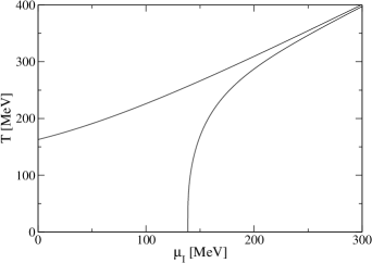
Figure 1: Phase diagram for pion condensation at the leading order. The upper curve is the chiral limit and the lower curve corresponds to the physical point.

We start with discussion of the choice of the parameters in the Lagrangian (1). First of all, in order for the theory to be stable, the bare coupling $\lambda_{b}$ has to be positive. This implies that the maximum value the cutoff $\Lambda$ may take at fixed renormalized coupling $\lambda$, is

$$\Lambda_{\text{max}}=\mu\exp\left(\frac{16\pi^{2}}{\lambda}\right).$$

In Refs. Andersen et al. (2004); Warringa (2006), it was shown that the mass of the sigma predicted by the model is maximal at $\lambda(\mu=100\text{ MeV})=80$, in which case $m_{\sigma}=433\text{ MeV}$, lying rather low in the experimentally observed range $m_{\sigma}=400-800\text{ MeV}$. However, for this large coupling the cutoff is forced to be unphysically small since $\Lambda_{\text{max}}=720\text{ MeV}$. We therefore choose a lower value, $\lambda(\mu=100\text{ MeV})=30$. The symmetry-breaking parameter $H$ is adjusted to $H=(104\text{ MeV})^{3}$ so that it, together with the pion decay constant $f_{\pi}=47\text{ MeV}$ (note that our definition of $f_{\pi}$ differs by a factor of $1/2$ from the standard value), reproduces the average of the measured masses of $\pi^{0},\pi^{\pm}$, $m_{\pi}=138\text{ MeV}$.

Note that for these values of the parameters, the sigma mass comes out as $m_{\sigma}=350\text{ MeV}$. The discrepancy with the measured value might be due to the fact that we restrict our treatment to the pion sector, and therefore miss contributions from the third-flavor physics. On the other hand, it might as well be just a shortcoming of the present approach.

With the above remark in mind, we plot in Fig. 1 the LO phase diagram both in the chiral limit and for the physical value of $H$. This phase diagram is identical to that found previously in Ref. Andersen (2007) using the 2PI effective action, because the leading orders of the 1PI and 2PI formalisms coincide. In Figs. 2 and 3 we show the dependence of the pion condensate on temperature and chemical potential, in the chiral limit and at the physical point, respectively.

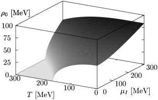
Figure 2: Pion condensate in the chiral limit as a function of temperature and chemical potential.

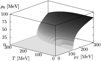
Figure 3: Pion condensate at the physical point as a function of temperature and chemical potential.

IV Next-to-leading order

IV.1 Effective potential

The NLO contribution to the effective potential is given by the second line of Eq. (8). By performing the Gaussian integral over the field $\chi$, we obtain

$$V_{\text{NLO}}=-\frac{1}{2}\hbox{$\sum$}\!\!\!\!\!\!\int_{P}\ln[I(P,M)]+\frac{1}{2}M^{2}a_{1}+\frac{1}{2}M^{4}b_{1}\\ -\frac{1}{2}\hbox{$\sum$}\!\!\!\!\!\!\int_{P}\ln\left[(P^{2}+m^{2})^{2}+4\mu_{I}^{2}\omega_{n}^{2}\right]+\hbox{$\sum$}\!\!\!\!\!\!\int_{P}\ln(P^{2}+M^{2}).$$ (18)

Here $I(P,M)$ is the inverse propagator of the $\alpha$-field in momentum space and reads

$$I(P,M)=\frac{1}{2}\Pi(P,M)+\frac{1}{\lambda}+b_{0}+\frac{\phi_{0}^{2}}{P^{2}+M^{2}}\\ +\frac{\rho_{0}^{2}(P^{2}+m^{2})}{(P^{2}+m^{2})^{2}+4\mu_{I}^{2}\omega_{n}^{2}}.$$ (19)

The last two terms of Eq. (18) represent the correction to the pressure of a free gas of charged scalar bosons, induced by finite chemical potential. It stems from the fact that at the leading order, $\phi_{1}$ and $\phi_{2}$ were treated on the same footing as all other fields, despite the fact that they are endowed with the chemical potential. The finite-temperature part of this correction (i.e., the difference of the Matsubara sum and the corresponding frequency integral) reduces to

$$\frac{T^{4}}{64\pi^{2}}\left[K_{0}^{+}(\beta M,\beta\mu_{I})+K_{0}^{-}(\beta M,\beta\mu_{I})-2J_{0}(\beta M)\right],$$

where the functions $K_{0}^{\pm}(\beta M,\beta\mu_{I})$ are the finite-$\mu_{I}$ generalizations of $J_{0}(\beta M)$,

$$K_{0}^{\pm}(\beta M,\beta\mu_{I})=\frac{32}{3T^{4}}\int_{0}^{\infty}dp\,\frac{p^{4}}{\omega_{p}}n(\omega_{p}\pm\mu_{I}).$$

On the other hand, the $T=0$ part of the last two terms of Eq. (18) gives, when evaluated with a four-dimensional cutoff, the contribution

$$\frac{1}{32\pi^{2}}\left(\mu_{I}^{2}\Lambda^{2}-\mu_{I}^{2}M^{2}+\frac{\mu_{I}^{4}}{6}\right).$$

This is clearly unphysical since it gives, among others, a $\mu_{I}$-dependent quadratic divergence. Should we use unconstrained integration over the frequency in combination with three-dimensional cutoff or dimensional regularization in $3-\epsilon$ space dimensions, we would get simply zero instead of these unpleasant terms Kapusta (1989). However, with these regularization schemes, which do not bound the size of the four-momentum, we would run into trouble with the self-energy $\Pi(P,M)$: As we will see shortly, it would turn negative at large enough $P^{2}$, due to the existence of the Landau pole in the running coupling. This clash of low-energy and high-energy physics prevents us from applying our method directly to the thermodynamics at nonzero chemical potential . Therefore, from now on we set $\mu_{I}=0$ and investigate the NLO corrections to the thermodynamics of chiral symmetry breaking. Moreover, at zero chemical potential we can, without lack of generality, set the pion condensate to zero, $\rho_{0}=0$.

The expression for the NLO effective potential (18) thus reduces just to the first term plus the counterterms. We first evaluate the self-energy function $\Pi(P,M)$, which is involved in the effective inverse propagator of the $\alpha$ field. Summing over Matsubara frequencies and integrating over three-momentum, we obtain

$$\Pi(P,M)=\frac{1}{16\pi^{2}}\left(\ln\frac{\Lambda^{2}}{M^{2}}+1+\sqrt{\frac{P^{2}+4M^{2}}{P^{2}}}\ln\frac{\sqrt{P^{2}+4M^{2}}-\sqrt{P^{2}}}{\sqrt{P^{2}+4M^{2}}+\sqrt{P^{2}}}\right)+\Pi_{T}(P,M),$$ (20)

where $\Pi_{T}(P,M)$ is the temperature-dependent part of the self-energy,

$$\Pi_{T}(P,M)=\frac{1}{8\pi^{2}p}\int_{0}^{\infty}dq\,\frac{q}{\omega_{q}}\ln\left(\frac{q^{2}+pq+A^{2}}{q^{2}-pq+A^{2}}\right)n(\omega_{q}),\quad A^{2}=\frac{P^{4}+4M^{2}p_{0}^{2}}{4P^{2}}.$$

The divergence in the expression (19) coming from the self-energy (20) is cancelled by the LO counterterm $b_{0}$.

Proceeding with the same steps as in Ref. Andersen et al. (2004), we next expand the self-energy in powers of $1/P^{2}$ in order to extract the dominant ultraviolet (UV) contributions. After averaging over angles, the UV-divergent part of the NLO effective potential stems from the part of the $\alpha$-propagator that we call $I_{\text{UV}}(P,M)$,

$$\ln[I_{\text{UV}}(P,M)]=\ln C_{1}+\frac{1}{P^{2}}\frac{C_{2}}{C_{1}}-\frac{1}{2P^{4}}\frac{C_{2}^{2}}{C_{1}^{2}}+\frac{1}{P^{4}}\frac{C_{3}}{C_{1}},$$

where

$$C_{1}= \ln\frac{\Lambda^{2}}{P^{2}}+\kappa,$$

$$C_{2}= 2(G-2M^{2})+2M^{2}C_{1},$$

$$C_{3}= -2M^{2}(G-\tfrac{M^{2}}{2})-2M^{4}C_{1},$$

and we have defined

$$\kappa =1+32\pi^{2}\left(\frac{1}{\lambda}+b_{0}\right),$$

$$G =16\pi^{2}\phi_{0}^{2}+T^{2}J_{1}(\beta M)-M^{2}\ln\frac{\mu^{2}}{M^{2}}-\frac{32\pi^{2}M^{2}}{\lambda}.$$

In order to avoid infrared (IR) singularity in the $1/P^{4}$ term, we make the replacement $P^{4}\to(P^{2}+\delta^{2})^{2}$ in the denominator, where $\delta$ is a small IR cutoff. Needless to say that this is just an artifact of the $1/P^{2}$ expansion and the full expression for the NLO effective potential, of course, does not depend on $\delta$. We next integrate $\ln[I_{\text{UV}}(P,M)]$ over $P$ and extract the UV-divergent part. The result can be written as

$$-\frac{1}{2}\int_{P}\ln[I_{\text{UV}}(P,M)]=D+\text{UV-finite pieces},$$ (21)

where the divergent terms are contained in

$$D\equiv\int_{P}\biggl{[}-\frac{1}{P^{2}}\biggl{(}M^{2}+\frac{G-2M^{2}}{\kappa+\ln\frac{\Lambda^{2}}{P^{2}}}\biggr{)}+\frac{2M^{4}}{(P^{2}+\delta^{2})^{2}}\biggr{]}\\ =\frac{1}{16\pi^{2}}\left[-M^{2}\Lambda^{2}+(G-2M^{2})\Lambda^{2}e^{\kappa}\operatorname{li}\frac{1}{e^{\kappa}}\right.\\ \left.+2M^{4}\left(\ln\frac{\Lambda^{2}}{\delta^{2}}-1\right)\right].$$ (22)

We have provided an exact representation of the divergence $D$, which is a necessity for the numerical implementation of renormalization.

IV.2 Renormalization

The UV-divergent term in Eq. (22), proportional to $G$, depends explicitly on temperature, except at the solution of the LO gap equation (14), where $G$ reduces to $16\pi^{2}f_{\pi}^{2}$. This led previously to the conclusion that the NLO effective potential is renormalizable in a temperature-independent manner only at the minimum Andersen et al. (2004). At this point, we should carefully distinguish what effective potential we are speaking of. It is crucial to note that what we have actually calculated so far, is not an effective potential of just the scalar fields $\phi_{i}$, but one of $\phi_{i}$ and $\alpha$.

As is clear already from the LO expression (10), such an effective potential does not have the usual physical interpretation as the minimum energy at fixed vacuum expectation values of the fields of the theory. In fact, it is unbounded from both below and above and the solution of the LO gap equations (13), (14) is its saddle point rather than a global extremum. This problem can be traced back to the fact that the field $\alpha$ is not an independent dynamical degree of freedom; upon using its equation of motion, it turns out to be a composite operator function of $\phi_{i}$.

The way out is to treat the gap equation for $M$ (12) as merely a constraint that serves to eliminate $M$ in favor of $\phi_{0}$. We thus arrive at an effective potential as a function solely of $\phi_{0}$, which already has the usual properties Coleman et al. (1974). This is the physical effective potential, $\mathcal{V}$, we eventually want to calculate, independent of the method we use.

First of all, let us note that none of the results of Sec. III is altered by changing the perspective from $V_{\text{LO}}(M,\phi_{0})$ to $\mathcal{V}_{\text{LO}}(\phi_{0})$. The reason is that, of course, the stationary point of $\mathcal{V}_{\text{LO}}$ coincides with that of $V_{\text{LO}}$ once the LO constraint (14) has been used to eliminate $M$ from it.

At the next-to-leading order we have to be more careful. Expanding the solution of the constraint (12) in powers of $1/N$ (and suppressing the argument in $M(\phi_{0})$ for the sake of legibility), the physical effective potential up to next-to-leading order reads,

$$\mathcal{V}(\phi_{0})=NV_{\text{LO}}(M_{\text{LO}}+\tfrac{1}{N}M_{\text{NLO}}+\dotsb,\phi_{0})+V_{\text{NLO}}(M_{\text{LO}}+\tfrac{1}{N}M_{\text{NLO}}+\dotsb,\phi_{0})\\ =NV_{\text{LO}}(M_{\text{LO}},\phi_{0})+\frac{\partial V_{\text{LO}}}{\partial M}(M_{\text{LO}},\phi_{0})M_{\text{NLO}}+V_{\text{NLO}}(M_{\text{LO}},\phi_{0})+\mathcal{O}(1/N)\\ =NV_{\text{LO}}(M_{\text{LO}},\phi_{0})+V_{\text{NLO}}(M_{\text{LO}},\phi_{0})+\mathcal{O}(1/N),$$

where the middle term vanishes due to the LO constraint (14). We can thus see that in order to calculate the physical effective potential to next-to-leading order, it is sufficient to solve the LO constraint for $M$. Doing that, we obtain the effective potential as a function of $\phi_{0}$ alone. Moreover, Eq. (22) tells us that the divergences of $\mathcal{V}_{\text{LO}}$ are independent of temperature for all values of $\phi_{0}$ since $G=16\pi^{2}f_{\pi}^{2}$ follows directly from the constraint (14) and does not need the true gap equation (13) to be fulfilled. Substituting for $G$, Eqs. (22) and (18) show that the necessary NLO counterterms are

$$a_{1}=\frac{\Lambda^{2}}{8\pi^{2}}\left(1+2e^{\kappa}\operatorname{li}\frac{1}{e^{\kappa}}\right),\quad b_{1}=-\frac{1}{4\pi^{2}}\ln\frac{\Lambda^{2}}{\mu^{2}}.$$ (23)

Finally, it is important to check whether the procedure of elimination of $M$ is in practice well defined. To this end, note that the left-hand side of Eq. (14) is a monotonically increasing function of $M^{2}$. It goes to $+\infty$ as $M^{2}\to+\infty$, and reaches the limit $f_{\pi}^{2}-\phi_{0}^{2}-\frac{T^{2}}{12}$ as $M^{2}\to 0$. This means that the constraint has a real solution only when $\phi_{0}$ is such that $\phi_{0}^{2}\geq f_{\pi}^{2}-\frac{T^{2}}{12}$. If this condition is satisfied, the solution of the constraint is unique as it should. Inside the interval $(-R,+R)$ around the origin with the “radius” $R=\sqrt{f_{\pi}^{2}-\frac{T^{2}}{12}}$, the effective potential $\mathcal{V}(\phi_{0})$ is undetermined by the auxiliary field technique. In principle it can be analytically continued to this interval Sher (1989) (this is what we actually do in our weak-coupling analysis in Sec. IV.3), but that would be hard to implement numerically. Fortunately, for our parameter set the minimum of the NLO effective potential always lies outside this interval so that the problem does not arise. It is also useful to note that the interval $(-R,+R)$ is precisely the region where the scalar field fluctuations become tachyonic, and the perturbative one-loop effective potential acquires nonzero imaginary part.

IV.3 Gap equations

Once we have renormalized the NLO effective potential, we may proceed in the standard manner and calculate the condensate $\phi_{0}$ as a solution to the gap equation,

$$\frac{d\mathcal{V}}{d\phi_{0}}=0.$$ (24)

Thanks to the fact that $M$ now depends on the condensate, we have to evaluate the total derivative using the chain rule, which leads to

$$\frac{\partial V_{\text{LO}}}{\partial\phi_{0}}+\frac{1}{N}\left(\frac{\partial V_{\text{NLO}}}{\partial\phi_{0}}+\frac{\partial V_{\text{NLO}}}{\partial M^{2}}\frac{\partial M_{\text{LO}}^{2}}{\partial\phi_{0}}\right)=0.$$ (25)

It is important to observe that while both $\partial V_{\text{NLO}}/\partial\phi_{0}$ and $\partial V_{\text{NLO}}/\partial M^{2}$ may in general contain temperature-dependent divergences (just because we can set $G=16\pi^{2}f_{\pi}^{2}$ only after taking the derivative), these cancel in the linear combination in Eq. (25).

To illustrate this procedure by an explicit example, let us consider the weak-coupling limit in case of exact chiral symmetry, i.e., $H=0$. Since $M=0$ in the chirally broken phase at the stationary point of the LO effective potential (10), we expect it to be of order $\mathcal{O}(\lambda)$ at the NLO value of the chiral condensate. Then, in the LO constraint (14) we can set $M=0$ everywhere except the term proportional to $1/\lambda$, which leads to the expression for $M$,

$$M^{2}=\frac{\lambda}{2}\left(-f_{\pi}^{2}+\phi_{0}^{2}+\frac{T^{2}}{12}\right).$$ (26)

The first partial derivative in Eq. (25) is simply $-M^{2}\phi_{0}$, while the last one is $\lambda\phi_{0}$ by Eq. (26). The $\mathcal{O}(\lambda)$ part of the derivative of $V_{\text{NLO}}$ with respect to $\phi_{0}$ is given by

$$\frac{\partial V_{\text{NLO}}}{\partial\phi_{0}}=-\phi_{0}\hbox{$\sum$}\!\!\!\!\!\!\int_{P}\frac{1}{P^{2}+M^{2}}\\ \times\frac{1}{\frac{1}{2}\Pi(P,M)+\frac{1}{\lambda}+b_{0}+\frac{\phi_{0}^{2}}{P^{2}+M^{2}}}\to-\lambda\phi_{0}\hbox{$\sum$}\!\!\!\!\!\!\int_{P}\frac{1}{P^{2}+M^{2}}.$$

By an analogous argument, the partial derivative with respect to $M^{2}$ is $\frac{1}{2}a_{1}+\mathcal{O}(\lambda)\to\Lambda^{2}/16\pi^{2}$ as $\lambda\to 0$. Putting all the pieces together, we find

$$\frac{d\mathcal{V}}{d\phi_{0}}=-M^{2}\phi_{0}-\frac{\lambda}{N}\phi_{0}\left(\hbox{$\sum$}\!\!\!\!\!\!\int_{P}\frac{1}{P^{2}+M^{2}}-\frac{\Lambda^{2}}{16\pi^{2}}\right)\\ =-\phi_{0}\left(M^{2}+\frac{\lambda}{N}\frac{T^{2}}{12}\right)+\mathcal{O}(\lambda^{2}).$$

The sum-integral above was calculated by differentiation of Eq. (9) with respect to $M^{2}$. This, together with the LO constraint (26), immediately yields the NLO expression for the chiral condensate in the weak-coupling limit,

$$\phi_{0}^{2}=f_{\pi}^{2}-\left(1+\frac{2}{N}\right)\frac{T^{2}}{12},$$

and the NLO critical temperature

$$T_{c}=\sqrt{\frac{12}{1+\frac{2}{N}}}f_{\pi}.$$ (27)

It is important to stress that while the LO critical temperature, $T_{c}=\sqrt{12}f_{\pi}$, derived in Sec. III.2 is a nonperturbative result valid for all values of the coupling, the present NLO correction is just a weak-coupling limit. In fact, while Eq. (27) predicts a decrease of the critical temperature with respect to the LO value, in particular for $N=4$ by about $20\%$, our numerical analysis discussed in Sec. IV.4 shows that at $\lambda(\mu=100\text{ MeV})=30$ the critical temperature actually increases by more than $30\%$! In order to make sure that these two results are consistent, we will briefly investigate the dependence of the critical temperature on the coupling.

Apart from calculating the exact minimum of the NLO effective potential, the NLO correction to the chiral condensate can also be determined in a more straightforward manner Veillette et al. (2007). One writes the solution to Eq. (24) as $\phi_{0}=\phi_{0}^{\text{LO}}+\frac{1}{N}\phi_{0}^{\text{NLO}}$ and expands the whole gap equation in powers of $1/N$. Comparing the terms of the same order, one thus gets an explicit formula for the NLO correction to the condensate,

$$\phi_{0}^{\text{NLO}}=-\frac{\frac{d\mathcal{V}_{\text{NLO}}(\phi_{0}^{\text{LO}})}{d\phi_{0}}}{\frac{d^{2}\mathcal{V}_{\text{LO}}(\phi_{0}^{\text{LO}})}{d\phi_{0}^{2}}}.$$ (28)

While the first derivative of the NLO effective potential in the numerator of Eq. (28) is best evaluated numerically, the second derivative of the LO effective potential in the denominator can be calculated analytically. Keeping in mind that this is a total derivative we find, in a fashion similar to Eq. (25),

$$\frac{d^{2}\mathcal{V}_{\text{LO}}}{d\phi_{0}^{2}}=\frac{\partial^{2}V_{\text{LO}}}{\partial\phi_{0}^{2}}-\left[\frac{\partial^{2}V_{\text{LO}}}{\partial(M^{2})^{2}}\right]^{-1}\left(\frac{\partial^{2}V_{\text{LO}}}{\partial\phi_{0}\partial M^{2}}\right)^{2}.$$

At the intermediate step, we used the implicit function theorem to extract the derivative $\partial M^{2}_{\text{LO}}/\partial\phi_{0}$ from the constraint (12). The second partial derivatives are easily found to be $\partial^{2}V_{\text{LO}}/\partial\phi_{0}^{2}=-M^{2}$, $\partial^{2}V_{\text{LO}}/\partial\phi_{0}\partial M^{2}=-\phi_{0}$, and

$$\frac{\partial^{2}V_{\text{LO}}}{\partial(M^{2})^{2}}=\frac{1}{32\pi^{2}}\left[J_{2}(\beta M)+\frac{32\pi^{2}}{\lambda}+\ln\frac{\mu^{2}}{M^{2}}-1\right],$$ (29)

where

$$J_{2}(\beta M)=-T^{2}\frac{dJ_{1}(\beta M)}{dM^{2}}=4\int_{0}^{\infty}dp\,\frac{n(\omega_{p})}{\omega_{p}}.$$

IV.4 Numerical results

For sake of numerical computation, the NLO effective potential was renormalized as follows. First, the “vacuum” effective potential, evaluated at zero temperature and with the LO value of the chiral condensate, was subtracted. This canceled the leading, quartic, field-independent divergence. In addition, we subtracted the integral representation of the remaining divergence (22). This amounts to NLO renormalization according to Eq. (23) as well as a finite piece, which must be added to the effective potential after the numerical integration,

$$\frac{M^{4}}{8\pi^{2}}\left(\ln\frac{\mu^{2}}{\delta^{2}}-1\right)-\frac{M_{0}^{4}}{8\pi^{2}}\left(\ln\frac{\mu^{2}}{\delta^{2}}-1\right),$$

where $M_{0}$ refers to the value of the mass parameter in the vacuum.

Note that the UV-finite pieces indicated in Eq. (21) depend explicitly on the counterterm $b_{0}$, hence also on the cutoff. It is technically advantageous to keep these terms and regulate the integrations with the cutoff even after all divergences have been subtracted. Physically this means that we treat our model as a low-energy effective theory and neglect contributions suppressed by inverse powers of the cutoff. In Ref. Andersen et al. (2004) the cutoff dependence of the final results was shown to be mild enough to justify this procedure. In concrete calculations, we chose $\Lambda=5\text{ GeV}$.

In Fig. 4 we display the numerical solution of the NLO gap equation (25) in the chiral limit. We can see that the correction to the chiral condensate is quite large. However, at zero temperature, the increase is about $25\%$, which is exactly what one would expect from a $1/N$ correction at $N=4$. The critical temperature increases from the LO value $163\text{ MeV}$ to $218\text{ MeV}$, which means an increase by about a third. That is still compatible with the $1/N$ prediction up to a numerical factor close to one.

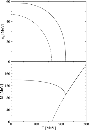
Figure 4: Solution of the NLO gap equation in the chiral limit. Upper panel: the chiral condensate; lower panel: the mass parameter $M$. For reference, the LO values are shown by the dashed lines.

At the physical point, the NLO corrections are considerably smaller, see Fig. 5. Here we also compare the exact self-consistent solution to the NLO gap equation (solid line) with the expansion of the condensate according to Eq. (28) (dash-dotted line). [In the chiral limit it cannot be used since the function $J_{2}(\beta M)$ diverges at the LO solution $M_{\text{LO}}=0$.] Apparently, the formula (28), though exact in the large-$N$ limit, is of little use in our case: At temperatures below about $200\text{ MeV}$, it overshoots the NLO correction to the condensate provided by exact solution to the gap equation (25) by nearly $100\%$. In spite of that, the two evaluations of the NLO condensate are formally consistent for their difference is of order $1/N^{2}$ of the LO value.

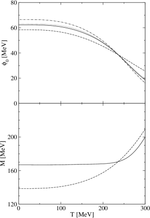
Figure 5: Solution of the NLO gap equation at the physical point (solid lines). Upper panel: the chiral condensate; lower panel: the mass parameter $M$. For reference, the LO values are shown by the dashed lines. We also show the NLO chiral condensate calculated using Eqs. (28) (dash-dotted) and (30) (dotted), respectively.

However, the agreement with the exact solution of the NLO gap equation can be improved by modifying Eq. (28) to

$$\phi_{0}^{\text{NLO}}=-\frac{\frac{d\mathcal{V}_{\text{NLO}}(\phi_{0}^{\text{LO}})}{d\phi_{0}}}{\frac{d^{2}\mathcal{V}_{\text{LO}}(\phi_{0}^{\text{LO}})}{d\phi_{0}^{2}}+\frac{1}{N}\frac{d^{2}\mathcal{V}_{\text{NLO}}(\phi_{0}^{\text{LO}})}{d\phi_{0}^{2}}}.$$ (30)

This expression is easily understood. The denominator contains the second derivative of the full (LO plus NLO) effective potential, and the numerator contains the first derivative of the same, just because $d\mathcal{V}_{\text{LO}}(\phi_{0}^{\text{LO}})/d\phi_{0}=0$. Eq. (30) then gives the approximate solution to the NLO gap equation by replacing the function $d\mathcal{V}/d\phi_{0}$ at the point $\phi_{0}=\phi_{0}^{\text{LO}}$ with a straight line; this is just the first step of the Newton iterative algorithm for solving nonlinear equations.

From the point of view of $1/N$ expansion, Eq. (30) resums a selected series of contributions to the gap from arbitrarily high orders. Our comparison to exact solution of the NLO gap equation demonstrates that Eq. (30) (dotted line in Fig. 5) is superior to the simpler expression (28) at a little extra computational cost (just one more evaluation of the NLO effective potential when implemented properly).

In order to make connection between our numerical results and the weak-coupling prediction (27) for the critical temperature in the chiral limit, we also investigated the dependence of the critical temperature on the renormalized coupling, with all other parameters fixed. The result is shown in Fig. 6. We could not check the limit (27) directly, because as follows from the discussion in Sec. IV.2, the auxiliary field technique only allows us to study the range of coupling for which the NLO critical temperature is higher than the LO one (and the chiral condensate at fixed temperature thus larger). Nevertheless, the plot in Fig. 6 clearly indicates that the critical temperature decreases at small coupling and the corresponding numerical values are consistent with the limit (27). (The bend at large coupling is most likely a cutoff effect: At $\lambda=40$ the maximal cutoff allowed by stability criterion is already very close to the actual value used in the computations.)

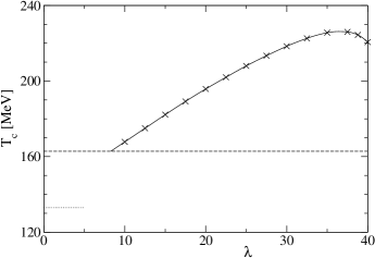
Figure 6: Critical temperature for chiral symmetry breaking as a function of the coupling. The dashed line denotes the LO critical temperature while the dotted one indicates the weak-coupling NLO limit (27).

In addition to the nonuniversal quantities such as the critical temperature and the condensate $\phi_{0}$ as a function of temperature, our NLO calculation also allows to check some universal properties of the $\mathrm{O}(N)$ model. At high temperature, the nonzero Matsubara modes decouple and the system undergoes dimensional reduction to a Euclidean field theory in three dimensions. This implies that the critical exponents of the system are those of the three-dimensional $\mathrm{O}(N)$ model. For example, the critical exponent $\nu$ that governs the behavior of the order parameter $\phi_{0}$ near the critical temperature, has been calculated in the $1/N$ expansion to next-to-leading order Alford et al. (2004); Zinn-Justin (2002),

$$\nu=\frac{1}{2}-\frac{4}{N\pi^{2}}+\mathcal{O}(1/N^{2}).$$

For $N=4$, this reduces to $\nu\approx 0.3987$ (as compared to the LO value $\nu=1/2$). The power-law fit based on the NLO chiral condensate in Fig. 4 is in agreement with this analytical result within the error bars.

V Conclusions

In the present paper, we have investigated the thermodynamics of the $\mathrm{O}(N)$ linear sigma model at the next-to-leading order of the 1PI-$1/N$ expansion. We explained how the NLO effective potential can be systematically renormalized in a temperature-independent manner. The crucial observation leading to this result was that the effective action previously used in literature, is one of the scalar field $\phi_{i}$ as well as the auxiliary composite field $\alpha$. The latter has to be eliminated before renormalization can be carried out consistently. One thus arrives at an effective action which is a function solely of $\phi_{i}$ and has the usual physical properties and interpretation. This procedure is further justified by the fact that in the numerical computation, we solved the NLO gap equation by direct extremization of the effective potential, thereby proving that the found solution provides a thermodynamically stable configuration.

A different way to calculate the NLO corrections to the condensates, based on expressions like (28), is sometimes used in the literature. This has the great advantage of being much less computationally demanding than the self-consistent solution of the NLO gap equations, in addition to the fact that the latter may lead to unphysical results Nikolic and Sachdev (2007). In our model the NLO gap equation can be solved exactly. A direct comparison of the results obtained using the two methods shows that a careless use of Eq. (28) can be misleading and need not improve the approximation provided by the leading order. We suggest a simple modification, Eq. (30), which in our case yields much better results with a little extra computational effort.

We also extended the NLO 1PI formalism to finite chemical potential. At leading order, we determined the phase diagram and confirmed the results previously obtained using the 2PI effective action at the leading order Andersen (2007). This is of course not surprising since at the leading order, the 1PI and 2PI formalisms coincide. It would be interesting to compare these two approaches at the next-to-leading order. In the present framework, we could not extend the explicit NLO calculations to finite chemical potential due to regularization problems. This issue as well as the relation to the 2PI formalism Aarts et al. (2002); Berges et al. (2005) will be subject of future work.