Sum-Capacity of Ergodic Fading Interference and Compound Multiaccess Channels

Abstract

The problem of resource allocation is studied for two-sender two-receiver fading Gaussian interference channels (IFCs) and compound multiaccess channels (C-MACs). The senders in an IFC communicate with their own receiver (unicast) while those in a C-MAC communicate with both receivers (multicast). The instantaneous fading state between every transmit-receive pair in this network is assumed to be known at all transmitters and receivers. Under an average power constraint at each source, the sum-capacity of the C-MAC and the power policy that achieves this capacity is developed. The conditions defining the classes of strong and very strong ergodic IFCs are presented and the multicast sum-capacity is shown to be tight for both classes.

I Introduction

The two-user interference channel (IFC) and the two-user compound multiaccess channel (C-MAC) model networks with two sources (senders or transmitters) and two destinations (receivers). The unicast case in which the message from each source is intended for only one destination is modeled as an IFC while the multicast case in which both messages are intended for both destinations is modeled as a C-MAC (see Fig. 1). The capacity region of a discrete memoryless C-MAC is obtained in [1]. The capacity region of both the discrete memoryless and the Gaussian IFC remain open problems; however, for certain classes of time-invariant IFCs satisfying specific well-defined constraints the capacity region is known (see for e.g., [2, 3, 4, 5] and the references therein).

The ergodic sum-capacity and the capacity region of a multiaccess channel (MAC) are studied in [6] and [7], respectively, under the assumption that the channel states and statistics are known at all nodes. These papers also develop the rate-optimal power policies. The ergodic capacity of a C-MAC, however, is not a straightforward extension of these results. For a parallel Gaussian IFC, in [8], the authors propose a sub-optimal iterative water-filling solution when every receiver views signals from the unintended transmitters as interference. In [9], the capacity of a parallel Gaussian IFC where every parallel subchannel is strong, i.e., its signal-to-noise and interference-to-noise ratios at each receiver satisfy specific conditions [2], is developed. In this paper, we study the problem of resource allocation for the two-user ergodic fading IFC and C-MAC under the assumption that the instantaneous fading state between each transmit-receive pair in this network is known at all transmitters and receivers. We develop the ergodic sum-capacity for the C-MAC which in turn lower bounds the sum-capacity of the IFC. We further develop the conditions defining the classes of strong and very strong ergodic IFCs with resource allocation and show that the C-MAC lower bounds are tight for both classes. Our work differs from [9] in that we develop capacity results for an ergodic IFC that is strong or very strong on average, i.e., the constraints for these classes require averaging over all channel instantiations, and thus, our result subsumes that in [9].

The sum-capacity optimal policy for the C-MAC is motivated by the work in [10] on maximizing the sum-rate of an ergodic fading two-user orthogonal multiaccess relay channel (MARC) [10] when the relay employs a decode-and-forward (DF) strategy. For the MARC, a DF relay acts as a decoding receiver; this enables us to generalize from [10] that when both receivers in a two-sender two-receiver network decode messages from both sources (users), the resulting sum-rate belongs to one of five disjoint cases or lies on the boundary of any two of them (boundary cases). Further, the sum-rate optimal policy either: 1) exploits the multiuser fading diversity to opportunistically schedule users analogous to the fading MAC [6, 7] or 2) involves simultaneous water-filling over two independent point-to-point links. We first develop the capacity region of the ergodic C-MAC; the resulting region is shown to lie within the capacity region of an ergodic IFC. The sum-rate optimal policy described above achieves the C-MAC sum-capacity and a lower bound on the IFC sum-capacity. We develop the conditions for the very strong IFC and show that the C-MAC lower bound for one of the five disjoint cases is tight for this IFC class. We define the conditions for the strong ergodic IFC and prove that when these conditions are met, the IFC sum-capacity is the C-MAC sum-capacity for one of three other disjoint cases or three boundary cases. We also show that, in contrast to the non-fading case [2], the constraints for both classes of IFC depend on both the channel statistics and average power constraints.

The paper is organized as follows. In Section II, we model the ergodic fading Gaussian C-MAC and IFC. In Section III we present the C-MAC capacity region and determine the power policies that maximize the sum-capacity. In Section IV, we define the strong and very strong ergodic IFC conditions and show that the sum-capacity in Section III is tight when the conditions for either the strong or the very strong ergodic IFC hold.

II Channel Model and Preliminaries

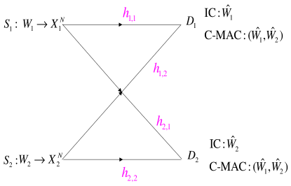
Figure 1: The two-user Gaussian IFC or C-MAC.

A two-sender two-receiver Gaussian IFC consists of two source nodes $S_{1}$ and $S_{2}$, and two destination nodes $D_{1}$ and $D_{2}$ as shown in Fig. 1. Source $S_{k}$, $k=1,2$, uses the channel $N$ times to transmit its messages $W_{k}$, distributed uniformly in the set $\,\{1,2,\ldots,2^{B_{k}}\}$, to its intended receiver, $D_{k}$, at a rate $R_{k}=B_{k}/N$ bits per channel use. In each use of the channel, $S_{k}$ transmits the signal $X_{k}$ while the destinations $D_{1}$ and $D_{2}$ receive $Y_{1}$ and $Y_{2}$, respectively, such that

$$Y_{1} =H_{1,1}X_{1}+H_{1,2}X_{2}+Z_{1}$$ (1)

$$Y_{2} =H_{2,1}X_{1}+H_{2,2}X_{2}+Z_{2}$$ (2)

where $Z_{1}$ and $Z_{2}$ are independent circularly symmetric complex Gaussian noise random variables with zero means and unit variances. For the special case when the messages at $S_{1}$ and $S_{2}$ are intended for both destinations, the model defined by (1) and (2) results in a two-user Gaussian C-MAC (see Fig. 1). We write $\mathbf{H}$ to denote the random matrix of fading states, $H_{k,m}$, for all $k,m=1,2$, such that $\mathbf{H}$ is a realization for a given channel use of a jointly stationary and ergodic (not necessarily Gaussian) fading process $\mathbf{H}$. Note that $H_{k,m}$ for all $k,m$, are not assumed to be independent. We also assume that over $N$ uses of the channel, the source transmissions are constrained in power according to

$$\left.\sum\limits_{i=1}^{N}\left|X_{k,i}\right|^{2}\leq N\overline{P}_{k}\right.\text{ for all }k=1,2$$ (3)

where $X_{k,i}$ denotes the transmitted signal from source $k$ in the $i^{th}$ channel use. Since the sources know the fading states of the links on which they transmit, they can allocate their transmitted signal power according to the channel state information. We write $P_{k}(\mathbf{H})$ to denote the power allocated at the $k^{th}$ transmitter as a function of the channel states $\mathbf{H}$. For an ergodic fading channel, (3) then simplifies to

$$\left.\mathbb{E}\left[P_{k}(\mathbf{H})\right]\leq\overline{P}_{k},\right.\text{ }k=1,2,$$ (4)

where the expectation in (4) is over the joint distribution of $\mathbf{H}$. We write $\underline{P}\left(\mathbf{H}\right)$ to denote a vector of power allocations with entries $P_{k}(\mathbf{H})$, for all $k$, and define $\mathcal{P}$ to be the set of all $\underline{P}\left(\mathbf{H}\right)$ whose entries satisfy (4). The capacity region $\mathcal{C}_{\text{IFC}}$ $\left(\mathcal{C}_{\text{C-MAC}}\right)$ of a two-user IFC (C-MAC) is defined as the closure of the set of rate tuples $(R_{1},R_{2})$ such that the destinations can decode their intended messages with an arbitrarily small positive error probability $\epsilon$. For ease of notation, we henceforth omit the functional dependence of $\underline{P}$ on $\mathbf{H}$. We write random variables (e.g. $H_{k,j}$) with uppercase letters and their realizations (e.g. $h_{k,j}$) with the corresponding lowercase letters. We write $\mathcal{K}=\left\{1,2\right\}$ to denote the set of transmitters, the notation $C(x)$ $=$ $\log(1+x)$ where the logarithm is to the base 2, $\left(x\right)^{+}=\max(x,0)$, and write $R_{\mathcal{S}}$ $=$ ${\textstyle\sum\nolimits_{k\in\mathcal{S}}}R_{k}$ for any ${\mathcal{S}}$ $\subseteq\mathcal{K}$.

III C-MAC: Sum-Capacity and Optimal Policy

The capacity region of a two-transmitter (sender) two-receiver discrete memoryless (d.m.) channel, now often referred to as a d.m. compound MAC, is developed in [1]. For each choice of input distribution at the two independent sources, this capacity region is an intersection of the MAC capacity regions achieved at the two receivers. The techniques in [1] can be easily extended to develop the capacity region for a Gaussian C-MAC with fixed channel gains. For the Gaussian C-MAC, one can show that Gaussian signaling achieves the capacity region using the fact that Gaussian signaling maximizes the MAC region at each receiver. Thus, the Gaussian C-MAC capacity region is an intersection of the Gaussian MAC capacity regions achieved at $D_{1}$ and $D_{2}$. For a stationary and ergodic process $\mathbf{H}$, the channel in (1) and (2) can be modeled as a set of parallel Gaussian C-MACs, one for each fading instantiation $H$. For the ergodic fading case, the capacity region $\mathcal{R}_{\text{C-MAC}}$, achieved over all $\underline{P}\in\mathcal{P}$ is given by the following theorem.

Theorem 1

The capacity region, $\mathcal{C}_{\text{C-MAC}}$, of an ergodic fading Gaussian C-MAC is

$$\mathcal{C}_{\text{C-MAC}}=\bigcup_{\underline{P}\in\mathcal{P}}\left\{\mathcal{C}_{1}\left(\underline{P}\right)\cap\mathcal{C}_{2}\left(\underline{P}\right)\right\}$$ (5)

where for all $\mathcal{S}\subseteq\mathcal{K}$ and $j=1,2,$ we have

$$\mathcal{C}_{j}\left(\underline{P}\right)=\left\{\left(R_{1},R_{2}\right):R_{\mathcal{S}}\leq\mathbb{E}\left[C\left(\sum_{k\in\mathcal{S}}\left|H_{j,k}\right|^{2}P_{k}\right)\right]\right\}.$$ (6)

Proof:

The achievability follows from using Gaussian signaling and decoding at both receivers. For the converse, we apply the proof techniques developed for the capacity of an ergodic fading MAC in [7]. For any $\underline{P}\in\mathcal{P}$, one can use limiting arguments (see for e.g., [7, Appendix B]) to show that for asymptotically error-free performance at receiver $j$, for all $j$, the achievable region has to be bounded as

$$\begin{array}[c]{cc}R_{\mathcal{S}}\leq\mathbb{E}\left[\log\left(1+\sum_{k\in\mathcal{S}}\left|H_{j,k}\right|^{2}P_{k}\right)\right],&j=1,2.\end{array}$$ (7)

The proof is completed by taking the union of the region over all $\underline{P}\in\mathcal{P}$. ∎

Corollary 2

The interference channel ergodic capacity region $\mathcal{C}_{\text{IFC}}$ is bounded as $\mathcal{C}_{\text{C-MAC}}\subseteq\mathcal{C}_{\text{IFC}}$.

Corollary 2 follows from the argument that a rate pair in $\mathcal{C}_{\text{C-MAC}}$ is achievable for the IFC since $\mathcal{C}_{\text{C-MAC}}$ is the capacity region when both messages are decoded at both receivers.

Remark 3

The capacity region $\mathcal{C}_{\text{C-MAC}}$ is convex. This follows from the convexity of the set $\mathcal{P}$ and the concavity of the $\log$ function.

The capacity region $\mathcal{C}_{\text{C-MAC}}$ is a union of the intersection of the pentagons $\mathcal{C}_{1}\left(\underline{P}\right)$ and $\mathcal{C}_{2}\left(\underline{P}\right)$ achieved at $D_{1}$ and $D_{2},$ respectively, where the union is over all $\underline{P}\in\mathcal{P}$. The region $\mathcal{C}_{\text{C-MAC}}$ is convex, and thus, each point on the boundary of $\mathcal{C}_{\text{C-MAC}}$ is obtained by maximizing the weighted sum $\mu_{1}R_{1}$ $+$ $\mu_{2}R_{2}$ over all $\underline{P}\in\mathcal{P}$, and for all $\mu_{1}>0$, $\mu_{2}>0$. Specifically, we determine the optimal policy $\underline{P}^{\ast}$ that maximizes the sum-rate $R_{1}+R_{2}$ when $\mu_{1}$ $=$ $\mu_{2}$ $=$ $1$. Using the fact that the rate regions $\mathcal{C}_{1}\left(\underline{P}\right)$ and $\mathcal{C}_{2}\left(\underline{P}\right)$ are pentagons, in Figs. 2 and 3 we illustrate the five possible choices for the sum-rate resulting from an intersection of $\mathcal{C}_{1}\left(\underline{P}\right)$ and $\mathcal{C}_{2}\left(\underline{P}\right)$ (see also [10]).

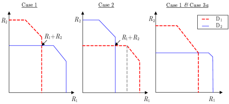
Figure 2: The rate region and sum-rate for cases $1$, $2$, and boundary case $(1,3a)$.

Figure 3: The rate region and sum-rate for cases $3a$, $3b$, and $3c$.

We broadly categorize the five possible choices for the sum-rate resulting from the intersection of two pentagons into the sets of active and inactive cases. The inactive set, consisting of cases $1$ and $2$, includes all intersections of $\mathcal{C}_{1}\left(\underline{P}\right)$ and $\mathcal{C}_{2}\left(\underline{P}\right)$ for which the constraints on the two sum-rates are not active, i.e., no rate tuple on the sum-rate plane achieved at one of the receivers lies within or on the boundary of the rate region achieved at the other receiver. On the other hand, the intersections for which there exists at least one such rate tuple such that the two sum-rates constraints are active belong to the active set. This includes cases $3a$, $3b$, and $3c$ shown in Fig. 2 where the sum-rate at $D_{1}$ is smaller, larger, or equal, respectively, to that achieved at $D_{2}$. By definition, the active set also include the boundary cases where there is exactly one such rate pair. However, to simplify the optimization problem, we consider the six boundary cases separately and denote them as cases $\left(l,n\right)$, $l=1,2,$ and $n=3a,3b,3c$. We write $\mathcal{B}_{i}\subseteq\mathcal{P}$ and $\mathcal{B}_{l,n}\subseteq\mathcal{P}$ to denote the set of power policies that achieve case $i$, $i=1,2,3a,3b,3c$ and case $\left(l,n\right)$, $l=1,2$, $n=3a,3b,3c$, respectively. Observe that cases $1$ and $2$ do not share a boundary since such a transition (see Fig. 2) requires passing through case $3a$ or $3b$ or $3c$. Finally, note that Fig. 3 illustrates two specific $\mathcal{C}_{1}$ and $\mathcal{C}_{2}$ regions for $3a$, $3b$, and $3c$.

The occurrence of any one of the disjoint cases depends on both the channel statistics and the policy $\underline{P}$. Since it is not straightforward to know a priori the power allocations that achieve a certain case, we maximize the sum-capacity for each case over all allocations in $\mathcal{P}$ and write $\underline{P}^{(i)}$ and $\underline{P}^{(l,n)}$ to denote the optimal solution for case $i$ and case $(l,n)$, respectively. Explicitly including boundary cases ensures that the sets $\mathcal{B}_{i}$ and $\mathcal{B}_{l,n}$ are disjoint for all $i$ and $(l,n)$, i.e., these sets are either open or half-open sets such that no two of them share a boundary (see [10]). This in turn simplifies the convex optimization as follows. Let $\underline{P}^{(i)}$ be the optimal policy maximizing the sum-rate for case $i$ over all $\underline{P}\in\mathcal{P}$. The optimal $\underline{P}^{(i)}$ must satisfy the conditions for case $i$, i.e., $\underline{P}^{(i)}$ $\in$ $\mathcal{B}_{i}$. If the conditions are satisfied, we prove the optimality of $P$⁽ⁱ⁾ using the fact that the rate functions for each case are concave. On the other hand, when $P$⁽ⁱ⁾ $\not\in$ $\mathcal{B}_{i}$, it can be shown that $R_{1}+R_{2}$ achieves its maximum outside $\mathcal{B}_{i}$. The proof again follows from the fact that $R_{1}+R_{2}$ for all cases is a concave function of $P$ for all $\underline{P}$ $\in$ $\mathcal{P}$. Thus, when $P$⁽ⁱ⁾ $\not\in$ $\mathcal{B}_{i}$, for every $P$ $\in$ $\mathcal{B}_{i}$ there exists a $P$^′ $\in$ $\mathcal{B}_{i}$ with a larger sum-rate. Combining this with the fact that the sum-rate expressions are continuous while transitioning from one case to another at the boundary of the open set $\mathcal{B}_{i}$, ensures that the maximum sum-rate is achieved by some $\underline{P}$ $\not\in$ $\mathcal{B}_{i}$. Similar arguments justify maximizing the optimal policy for each case over all $\mathcal{P}$.

The following theorem summarizes the optimal power policy for each case. The optimal $\underline{P}^{\left(i\right)}$ or $\underline{P}^{\left(l,n\right)}$ maximizing the sum-rate for case $i$ or $\left(l,n\right)$ satisfies the conditions for only that case and is determined using Lagrange multipliers and the Karush-Kuhn-Tucker (KKT) conditions.

Theorem 4

A policy $\underline{P}^{\left(i\right)}$ or $\underline{P}^{\left(l,n\right)}$ maximizes the sum-rate for case $i$, $i=1,2,3a,3b,3c,$ or the boundary case $\left(l,n\right)$, $l=1,2$, and $n=3a,3b,3c,$ when the entries $P$${}_{1}^{\left(\cdot\right)}$ and $P$${}_{2}^{\left(\cdot\right)}$ of $\underline{P}^{\left(\cdot\right)}$ satisfy

$$\begin{array}[c]{cc}f_{k}^{\left(\cdot\right)}\leq\nu_{k}\ln 2&k=1,2\end{array}$$ (8)

where $\nu_{k}$ is chosen to satisfy (4) such that

$$\begin{array}[c]{ll}f_{k}^{(i)}=\frac{\left|h_{m,k}\right|^{2}}{\left(1+\left|h_{m,k}\right|^{2}P_{k}\right)}&\begin{array}[c]{c}i=1:\left(m,k\right)=(1,1),(2,2)\\ i=2:\left(m,k\right)=(1,2),(2,1)\end{array}\\ f_{k}^{(i)}=\frac{\left|h_{m,k}\right|^{2}}{\left(1+\sum_{j=1}^{2}\left|h_{m,j}\right|^{2}P_{j}\right)}&\begin{array}[c]{c}i=3a:m=1\\ i=3b:m=2\end{array}\end{array}$$ (9)

$$\begin{array}[c]{ll}\begin{array}[c]{l}f_{k}^{\left(i\right)}=\left(1-\alpha\right)f_{k}^{\left(3a\right)}\\ ~{}\ \ \ \ \ \ \ \ \ +\alpha f_{k}^{\left(3b\right)}\end{array}&\text{ }i=3c\\ \begin{array}[c]{l}f_{k}^{\left(l,n\right)}=\left(1-\alpha\right)f_{k}^{\left(n\right)}\\ \text{ \ \ \ \ \ \ \ \ \ \ }+\alpha f_{k}^{\left(l\right)}\text{ \ \ \ \ \ \ }\end{array}&\left(l,n\right)=(1,3a),(2,3b)\\ \begin{array}[c]{l}f_{k}^{\left(l,3c\right)}=\alpha_{3}f_{k}^{\left(3a\right)}\\ \text{ \ \ \ \ \ \ \ \ \ }+\alpha_{2}f_{k}^{\left(3b\right)}+\alpha_{1}f_{k}^{(l)}\end{array}&l=1,2\end{array}$$ (10)

with $\alpha$, $\alpha_{1}$, $\alpha_{2}$, and $\alpha_{3}=1-\alpha_{1}-\alpha_{2}$ chosen to satisfy the appropriate boundary conditions. The optimal $\underline{P}^{\left(i\right)}\in\mathcal{B}_{i}$ or $\underline{P}^{\left(l,n\right)}\in\mathcal{B}_{l,n}$ satisfies the condition for case $i$ or case $(l,n)$, respectively. The conditions for each case are given as

$$\begin{array}[c]{cc}\text{Case }1:&\begin{array}[c]{c}I(X_{1};Y_{1}|X_{2}\mathbf{H})<I(X_{1};Y_{2}|\mathbf{H})\\ I(X_{2};Y_{2}|X_{1}\mathbf{H})<I(X_{2};Y_{1}|\mathbf{H})\end{array}\end{array}$$ (14)

$$\begin{array}[c]{cc}\text{Case }2:&\begin{array}[c]{c}I(X_{1};Y_{1}|X_{2}\mathbf{H})<I(X_{1};Y_{2}|\mathbf{H})\\ I(X_{2};Y_{2}|X_{1}\mathbf{H})<I(X_{2};Y_{1}|\mathbf{H})\end{array}\end{array}$$ (18)

$$\begin{array}[c]{cc}\text{Case }3a:&I(X_{1}X_{2};Y_{1}|\mathbf{H})<I(X_{1}X_{2};Y_{2}|\mathbf{H})\end{array}$$ (20)

$$\begin{array}[c]{cc}\text{Case }3b:&I(X_{1}X_{2};Y_{1}|\mathbf{H})>I(X_{1}X_{2};Y_{2}|\mathbf{H})\end{array}$$ (22)

$$\begin{array}[c]{cc}\text{Case }3c:&I(X_{1}X_{2};Y_{1}|\mathbf{H})=I(X_{1}X_{2};Y_{2}|\mathbf{H})\end{array}$$ (24)

$$\begin{array}[c]{cc}\text{Case }\left(l,n\right):&\begin{array}[c]{c}\text{Satisfy cases }n\text{ }\&\text{ }l\text{ with }\\ \text{equality for one case }l\text{ condition }\end{array}\end{array}$$ (25)

where in (14)-(25), $X_{1}$ and $X_{2}$ are Gaussian distributed subject to (4). The $\underline{P}^{\ast}$ that maximizes the sum-capacity is obtained by computing $\underline{P}^{(i)}$ or $\underline{P}^{(l,n)}$ starting with the inactive cases, followed by the boundary cases $(l,n)$, and finally the active cases $3a,$ $3b,$ and $3c$ until for some case the corresponding $\underline{P}^{(i)}$ or $\underline{P}^{(l,n)}$ satisfies the case conditions.

From (8) and (9), one can easily verify that for the inactive cases $1$ and $2$ the optimal policies involve the classic water-filling solution over point-to-point links. Specifically, the optimal policies for cases $1$ and $2$ simplify to water-filling over the two bottle-neck links $(S_{1}\rightarrow D_{1})$, $(S_{2}\rightarrow D_{2})$ and $(S_{1}\rightarrow D_{2})$, $(S_{2}\rightarrow D_{1})$, respectively. On the other hand, for the active cases $3a$ and $3b$, the optimal allocation at each source simplifies to the opportunistic water-filling allocation for a MAC [6, 7] such that in each channel use the source with the larger $f_{k}^{\left(i\right)}/\nu_{k}$ for case $i,$ $i=3a,3b$, transmits. Observe that the water-filling solutions are with respect to the receiver that achieves the smaller sum-capacity. Finally, for all the boundary cases including case $3c$, the optimal policy for source $k$ is still an opportunistic solution such that the source with the larger $f_{k}^{(i)}/\nu_{k}$ or $f_{k}^{(l,n)}/\nu_{k}$, $i=3c$ and for all $(l,n)$, transmits. However, unlike the other cases, the optimal policy at each source for the boundary cases is no longer a water-filling solution; instead for each channel instantiation the optimal policy at source $k$ satisfies (8) with equality when the users are opportunistically scheduled.

The conditions in (14) and (18) for the two inactive cases exclude all other cases and define the disjoint sets $\mathcal{B}_{1}$ and $\mathcal{B}_{2}$. Similarly, the conditions for the six boundary cases define the disjoint sets $\mathcal{B}_{l,n}$ for all $\left(l,n\right)$. However, the conditions for $3a$, $3b$, and $3c$ can be satisfied by the boundary cases. To ensure that the sets $\mathcal{B}_{3a}$, $\mathcal{B}_{3b}$, and $\mathcal{B}_{3c}$ are disjoint from all other sets, the algorithm for determining the optimal $P$^∗ requires eliminating a case at a time starting from case $1$. Thus, the algorithm first eliminates the inactive cases, and then checks for the boundary cases, and finally checks for cases $3a,$ $3b$, and $3c$.

Remark 5

The capacity region, $\mathcal{C}_{\text{C-MAC}}$ can be completely characterized by using the same approach to maximize the sum $\mu_{1}R_{1}+\mu_{2}R_{2}$, for all $\left(\mu_{1},\mu_{2}\right)$ pairs. In general, each tuple on the boundary of $\mathcal{C}_{\text{C-MAC}}$ may be maximized by a different case, and thus, the optimal policy is also a function of $\left(\mu_{1},\mu_{2}\right)$.

IV IFC: Converse

We now apply the results in Theorem 4 to the ergodic fading IFC. For the IFC, the power policies satisfying (8) and (9) are achievable when $D_{1}$ and $D_{2}$ decode messages from both sources; the resulting C-MAC sum-capacity is a lower bound on the IFC sum-capacity. Below, we present a converse to show that these sum-rate lower bounds are tight for the classes of strong and very strong ergodic fading IFC. The convex capacity region of the ergodic fading two-user IFC, $\mathcal{C}_{\text{IFC}}$, can be bounded by hyperplanes $C\left(\mu_{1},\mu_{2}\right)$ such that for all $\mu_{1}>0$ and $\mu_{2}>0$, we have

$$\mathcal{C}_{\text{IFC}}=\left\{\left(R_{1},R_{2}\right):\mu_{1}R_{1}+\mu_{2}R_{2}\leq C\left(\mu_{1},\mu_{2}\right)\right\}$$ (26)

subject to (4). The boundary of $\mathcal{C}_{\text{IFC}}$ is determined by maximizing $\mu_{1}R_{1}+\mu_{2}R_{2}$ for each choice of $(\mu_{1},\mu_{2})$ over all $\underline{P}\in\mathcal{P}$. For the sum-capacity, we set $\mu_{1}=\mu_{2}=1$.

IV-A Very Strong Ergodic IFC

Definition 6

A very strong ergodic fading IFC with respect to the tuple $\left(\mu_{1},\mu_{2}\right)$ results when a $\underline{P}\in\mathcal{P}$ and $\mathbf{H}$ satisfy

$$\begin{array}[c]{c}I(X_{1};Y_{1}|X_{2}\mathbf{H})<I(X_{1};Y_{2}|\mathbf{H})\\ I(X_{2};Y_{2}|X_{1}\mathbf{H})<I(X_{2};Y_{1}|\mathbf{H})\end{array}$$ (27)

for all choices of $X_{1}$ and $X_{2}$.

Theorem 7

The sum-capacity of a class of very strong ergodic Gaussian IFCs is

$$\sum_{k=1}^{2}\mathbb{E}\left[\log\left(1+\left|H_{k,k}\right|^{2}P_{k}^{\ast}\left(\mathbf{H}\right)\right)\right]$$ (28)

where $P$${}_{k}^{\ast}\left(\mathbf{H}\right)$, for all $k$, is the optimal water-filling solution for single-sender single-receiver ergodic fading links.

Proof:

An outer bound on the sum-capacity of the IFC can be obtained by setting $H_{j,k}=0$ for all $j\not=k$, i.e., by assuming no interference. In the absence of interference, Gaussian signaling achieves capacity for each of the $S_{k}$ to $D_{k}$ links, $k=1,2$, and the resulting sum-capacity is given by (28) where, $P$${}_{k}^{\ast}\left(\mathbf{H}\right)$ is the optimal water-filling solution for single-sender single-receiver ergodic fading links, i.e., it satisfies the condition in (8) for $f_{k}^{(1)}$ in (9), subject to (4). From Theorem 4, we see that when the channel statistics and the power policy satisfy (14), i.e., $\underline{P}^{\ast}=\underline{P}^{(1)}\in\mathcal{B}_{1}$, the achievable strategy of decoding both messages at both destinations achieves this sum-capacity outer bound. Thus, the sum-capacity of a very strong IFC is that of a C-MAC for which $\underline{P}$ satisfies case $1$ conditions, i.e., $\underline{P}$ satisfies (27). ∎

For a deterministic $\mathbf{H}$, the conditions in (27) simplify to those for the very strong non-fading IFC in [2]. Further, from Fig. 2, we see that as with the non-fading very strong IFC, the intersecting region for Case $1$ is also a rectangle; note, however that unlike the non-fading case, this rectangle is not the entire capacity region but only the region achieving the sum-capacity. Finally, note that the condition in (27) depends on both the channel statistics and the transmit power.

Remark 8

In contrast, the conditions for case $2$ in (18) model a weak ergodic IFC for which the C-MAC sum-capacity is strictly a lower bound.

IV-B Strong Ergodic IFC

Definition 9

A strong ergodic fading IFC with respect to the tuple $\left(\mu_{1},\mu_{2}\right)$ results when a $\underline{P}\in\mathcal{P}$ and $\mathbf{H}$ satisfies

$$I(X_{1};Y_{1}|X_{2}\mathbf{H}) <I(X_{1};Y_{2}|X_{2}\mathbf{H})$$ (29)

$$I(X_{2};Y_{2}|X_{1}\mathbf{H}) <I(X_{2};Y_{1}|X_{1}\mathbf{H})$$ (30)

for all choices of $X_{1}$ and $X_{2}$.

Theorem 10

The sum-capacity of the class of strong ergodic fading Gaussian IFCs is

$$\min_{j=1,2}\left\{\mathbb{E}\left[C\left(\sum\nolimits_{k=1}^{2}\left|H_{j,k}\right|^{2}P_{k}^{\ast}\right)\right]\right\}$$ (31)

where, for all $k$, $P_{k}^{\ast}=P_{k}^{\left(i\right)}$ or $P_{k}^{\ast}=P_{k}^{\left(l,n\right)}$ for $l=1$ and $i,n\in\left\{3a,3b,3c\right\}$.

Proof:

Due to lack of space, we present a proof sketch. We use the fact that the channel states are independent of the source messages, Fano’s and the data processing inequality, the ergodicity of the channel for large $N$, the fact that $\underline{P}\in\mathcal{P}$ satisfies (29) and (30), and the optimality of Gaussian signaling to upper bound the sum-rate as

$$R_{1}+R_{2} \leq\left[I(X_{1};Y_{1}|X_{2}\mathbf{H})+I(X_{2};Y_{2}|\mathbf{H})\right]$$ (32)

$$\leq\left[I(X_{1};Y_{2}|X_{2}\mathbf{H})+I(X_{2};Y_{2}|\mathbf{H})\right]$$ (33)

$$\leq I(X_{1}X_{2};Y_{2}|\mathbf{H})$$ (34)

$$\leq\mathbb{E}\left[C\left(\sum\nolimits_{k=1}^{2}\left|H_{2,k}\right|^{2}P_{k}^{\ast}\right)\right]$$ (35)

One can similarly show that

$$R_{1}+R_{2}\leq\mathbb{E}\left[C\left(\sum\nolimits_{k=1}^{2}\left|H_{1,k}\right|^{2}P_{k}^{\ast}\right)\right],$$ (36)

and thus, from (6) we see that the sum-rate is upper bounded by the sum-capacity of a C-MAC. Further, we can bound $R_{1}\leq\mathbb{E[}C(\left|H_{1,k}\right|^{2}P_{k}^{\ast})]$ and $R_{2}\leq$ $\mathbb{E[}C(\left|H_{2,k}\right|^{2}P_{k}^{\ast})]$, and thus, from Corollary 2, the sum-capacity of a the ergodic C-MAC sum-capacity is also the sum-capacity of the ergodic IFC when (29) and (30) hold.

Optimal Power Allocation : From Theorem 4, the optimal $\underline{P}^{\ast}$ for an ergodic C-MAC satisfies only one of the conditions in (14)-(25). Further, from Theorem 4 and Figs. 2 and 3, the conditions in (29) and (30) can be satisfied by $7$ different cases, namely, cases $1$, $3a$, $3b$, $3c$, $\left(1,3a\right)$, $\left(1,3b\right)$, and $\left(1,3c\right)$. Since these cases are mutually exclusive, the optimal $\underline{P}^{\ast}$ is given by that optimal policy which in addition to satisfying the condition for one of the above listed cases also satisfies (29) and (30). For example, suppose $\underline{P}^{\ast}$ satisfies the condition for case $1$, i.e., $\underline{P}^{\ast}\in\mathcal{B}_{1}$. Since the conditions for this very strong case in (14) (see also (27)) imply the conditions for the strong case in (29) and (30), the sum-capacity and the optimal power policy are directly given by Theorem 7. On the other hand, suppose $\underline{P}^{\ast}\in\mathcal{B}_{3a}$, i.e., $\underline{P}^{\ast}$ satisfies the conditions in Theorem 4 only for case $3a$ (see Fig. 3). Since $\underline{P}^{\ast}$ also satisfies (29) and (30), we define an open (or half-open) set $\mathcal{B}_{3a}^{\prime}\subset\mathcal{B}_{3a}$ in which (29), (30), and (20) are all satisfied. The concavity of the sum-rate expression for this case then guarantees that the optimal policy is unique and belongs to the open set $\mathcal{B}_{3a}^{\prime}$ (see also the arguments in Section III). Note that the requirement that $\underline{P}^{(3a)}$ satisfy (29) and (30) only limits $\underline{P}^{(3a)}$ to $\mathcal{B}_{3a}^{\prime}$ and does not change the solution presented in Theorem 4 for this case. Thus, the sum-capacity for this case is

$$\mathbb{E}\log\left(1+\sum_{k=1}^{2}\left|H_{1,k}\right|^{2}P_{k}^{(3a)}\left(\mathbf{H}\right)\right).$$ (37)

The arguments above also apply to the remaining cases listed above. ∎

Remark 11

The conditions in (29) and (30) are ergodic generalizations of the conditions presented in [2] for the non-fading strong IFC (see also [4, (1),(2)] for the discrete memoryless strong IFC). However, unlike the non-fading Gaussian IFC, the conditions in (29) and (30) for the ergodic Gaussian IFC depend on both the channel statistics and the power policy $\underline{P}$. Further, as expected, the very strong ergodic IFC is a special case of the strong IFC where (27) holds.

References

- [1] R. Ahlswede, “The capacity region of a channel with two senders and two receivers,” Ann. Prob., vol. 2, pp. 805–814, Oct. 1974.
- [2] H. Sato, “The capacity of Gaussian interference channel under strong interference,” IEEE Trans. Inform. Theory, vol. 27, no. 6, pp. 786–788, Nov. 1981.
- [3] A. B. Carleial, “A case where interference does not reduce capacity,” IEEE Trans. Inform. Theory, vol. 21, no. 5, pp. 569–570, Sept. 1975.
- [4] M. H. M. Costa and A. El Gamal, “The capacity region of the discrete memoryless interference channel with strong interference,” IEEE Trans. Inform. Theory, vol. 33, no. 5, pp. 710–711, Sept. 1987.
- [5] A. Motahari and A. Khandani, “Capacity bounds for the Gaussian interference channel,” Jan. 2008, submitted to the IEEE Trans. Inform. Theory.
- [6] R. Knopp and P. Humblet, “Information capacity and power control in single-cell multiuser communications,” in Proc. IEEE Intl. Conf. Commun., Seattle, WA, June 1995.
- [7] D. N. C. Tse and S. V. Hanly, “Multiaccess fading channels - part I: Polymatroid structure, optimal resource allocation and throughput capacities,” IEEE Trans. Inform. Theory, vol. 44, no. 7, pp. 2796–2815, Nov. 1998.
- [8] W. Yu, G. Ginis, and J. M. Cioffi, “Distributed multiuser power control for digital subscriber lines,” IEEE J. Sel. Areas Commun., vol. 20, no. 5, pp. 1105–1115, June 2002.
- [9] S. T. Chung and J. M. Cioffi, “The capacity region of frequency-selective gaussian interference channels under strong interference,” IEEE Trans. Comm., vol. 55, no. 9, pp. 1812–1820, Sept. 2007.
- [10] L. Sankar, Y. Liang, H. V. Poor, and N. B. Mandayam, “Opportunistic communications in orthogonal multiaccess relay channels,” in Proc. Int. Symp. Inf. Theory, Nice, France, July 2007.