Fragmentation of Shocked Flows: Gravity, Turbulence and Cooling

Abstract

The observed rapid onset of star formation in molecular clouds requires rapid formation of dense fragments which can collapse individually before being overtaken by global gravitationally-driven flows. Many previous investigations have suggested that supersonic turbulence produces the necessary fragmentation, without addressing however the source of this turbulence. Motivated by our previous (numerical) work on the flow-driven formation of molecular clouds, we investigate the expected timescales of the dynamical and thermal instabilities leading to the rapid fragmentation of gas swept up by large-scale flows, and compare them with global gravitational collapse timescales. We identify parameter regimes in gas density, temperature and spatial scale within which a given instability will dominate. We find that dynamical instabilities disrupt large-scale coherent flows via generation of turbulence, while strong thermal fragmentation amplifies the resulting low-amplitude density perturbations, thus leading to small-scale, high-density fragments as seeds for local gravity to act upon. Global gravity dominates only on the largest scales; large-scale gravitationally-driven flows promote the formation of groups and clusters of stars formed by turbulence, thermal fragmentation, and rapid cooling.

1. Motivation

There is increasing evidence that star formation (in the solar neighborhood) follows rapidly on molecular cloud formation (Hartmann et al., 2001; Ballesteros-Paredes & Hartmann, 2007; Elmegreen, 2007). This evidence suggests that the density enhancements in which stars form are produced during the cloud formation phase – and not after the cloud has formed, as implicitly assumed by the initial conditions of many numerical models. Global gravitational modes can sweep up material at the edges of clouds (Burkert & Hartmann, 2004), leading to the formation of filaments (Vázquez-Semadeni et al., 2007; Heitsch et al., 2008). Yet for local gravitational collapse to win, the cloud needs to be seeded with local perturbations early on (Burkert & Hartmann, 2004; Hartmann & Burkert, 2007). Not only need these density enhancements to arise early, but they also need to be non-linear, i.e. the cloud must acquire strong small-scale density perturbations during its formation. Thus, a rapid fragmentation mechanism other – and faster! – than gravity is needed.

The scenario of flow-driven cloud formation, in which large-scale shocked flows of atomic hydrogen in the warm neutral medium (WNM) assemble molecular clouds (Ballesteros-Paredes et al., 1999; Hartmann et al., 2001), offers an elegant mechanism for the rapid fragmentation of the proto-cloud and the generation of non-linear density seeds. The key to the rapid fragmentation is a combination of strong dynamical and thermal instabilities in shocked flows (Hennebelle & Pérault, 1999 and Koyama & Inutsuka, 2000 for one-dimensional models; Koyama & Inutsuka, 2002 for 2D models including H₂ formation; Audit & Hennebelle, 2005, Heitsch et al., 2005, 2006, Hennebelle & Audit, 2007 and Hennebelle et al., 2007 emphasizing the formation of cold neutral medium clouds in 2D; Vázquez-Semadeni et al., 2006, Vázquez-Semadeni et al., 2007 and Heitsch et al., 2008 for three-dimensional models, the latter two including self-gravity). Rather than generating turbulence by imposing e.g. a velocity field chosen ad hoc in Fourier space, density and velocity structures arise naturally during the formation of the cloud in this scenario.

In this study, we attempt to throw some light on the relative importance of various classes of instabilities at play, via a consideration of their timescales. We aim to assess whether fragmentation processes other than gravity are acting rapidly enough during the formation of molecular clouds to allow the rapid onset of local star formation. Thermal effects – strong cooling and thermal instability (TI, Field, 1965) play a dominant role, weakening the effective equation of state in a shocked flow and thus allowing rapid fragmentation. The TI derives its strength from a combination with turbulence which generates density perturbations on small scales. The resulting rapid growth of small-scale perturbations allows the rapid onset of local gravitational collapse, before global collapse modes overwhelm any pre-existing low-amplitude density variations. Hence, in the context of flow-driven cloud formation, thermal fragmentation is the key to the rapid onset of star formation.

The expressions for the timescales and the instability conditions are given in §2. We discuss the parameter regimes for the instabilities and their consequences in §3 and summarize in §4.

2. Timescales and Instability Conditions

The instabilities enabling the rapid fragmentation of shocked flows are associated with characteristic timescales. These will serve as a vehicle to estimate the relative importance of the instabilities for fragmentation and turbulence generation.

Since we are mainly interested in the competition between global gravity and local fragmentation processes, we restrict ourselves to the discussion of four instabilities which can be split into two groups of physical processes, namely condensation processes (driven by cooling [§2.1] and gravity [§2.2]) and generic fluid instabilities (ram pressure imbalance [§2.3] and shear flows [§2.4]). This list of instabilities is by no means exhaustive (§2.5). Our choice is to some extent guided by the results of our numerical simulations (Heitsch et al., 2008), and by the notion of cloud formation in large-scale, organized flows such as spiral arms of galaxies (Kim et al., 2003; Kim & Ostriker, 2006; Elmegreen, 2007; Dobbs & Bonnell, 2007, 2008), or expanding supernova shells (e.g. Elmegreen & Lada, 1977; see also discussion in Ballesteros-Paredes & Hartmann, 2007).

2.1. Thermal Instability (TI) and Cooling Timescales

The TI rests on the balance between heating and cooling processes. The astrophysically most relevant mode is the isobaric condensation mode (e.g. Balbus, 1995). The condensation mode’s linear growth rate is independent of the wave number as long as the perturbation can adjust to an isobaric state and under neglection of heat conduction, however, perturbations on smaller scales will grow first (Burkert & Lin, 2000). Thus, in the linear regime, the condensation mode is limited to scales smaller than the sound crossing length (see also Vázquez-Semadeni et al., 2003 and Hennebelle & Audit, 2007),

$$\lambda_{c}=\tau_{c}\,c_{s},$$ (1)

where

$$\tau_{c}=\frac{k_{B}T}{n\Lambda}$$ (2)

is the cooling timescale with temperature $T$ and particle density $n$. Thermal energy losses due to optically thin, collisionally excited atomic lines are given by the cooling function $\Lambda(T)$ in erg cm³ s^-1. The sound speed is

$$c_{s}\equiv\sqrt{\frac{\gamma k_{B}T}{\mu}},$$ (3)

with the mean molecular mass $\mu$. Since the TI spans a range of 2 orders of magnitude in temperature, condition (1) can become quite restrictive, but it varies strongly with temperature and the strength of the cooling (see Fig. 1). The scale $\lambda_{c}$ can drop to a few tenths of a parsec for parameters typical of the WNM.

In the non-linear regime, and on scales $\lambda>\lambda_{c}$, the gas can still cool isochorically such that the resulting pressure drop will generate waves (e.g. Balbus, 1995), leading to additional fragmentation. In that sense, equation (1) is not a strict upper limit for the TI, since it only refers to the (linear) evolution of the condensation mode. Nevertheless, we will use it as a proxy for estimating the importance of the TI since it gives the largest scale out of which a single coherent cold fragment can form and thus is emphasizing the local nature of the TI. On small scales, the condensation mode is limited by the Field (1965) length, below which heat conduction will become important (see e.g. Koyama & Inutsuka, 2004). The condensation mode will grow if

$$\left(\frac{\partial{\cal L}}{\partial T}\right)_{n}-\frac{n_{0}}{T_{0}}\left(\frac{\partial{\cal L}}{\partial n}\right)_{T}<0,$$ (4)

where ${\cal L}\equiv n\Lambda-\Gamma$ is the loss-heat function in erg s^-1 (Field, 1965).

The growth timescale of the condensation mode under the conditions (1) and (4) is given by

$$\tau_{TI}\equiv\frac{\gamma\,k_{B}\,T}{(\gamma-1)(n\,\partial{\cal L}_{n}-T\,\partial{\cal L}_{T})}$$ (5)

with the partial derivatives $\partial{\cal L}_{n}\equiv\partial{\cal L}/\partial n$ and $\partial{\cal L}_{T}\equiv\partial{\cal L}/\partial T$. Equation (5) includes the condition for the condensation mode, i.e. for $\tau_{TI}<0$, the condensation mode does not grow.

Thermal effects still may be important in the absence of the TI, in which case the thermal timescale is given by the more general cooling time (eq. [2]). A short $\tau_{c}$ does not necessarily entail TI. Rather, a short $\tau_{c}$ in the presence of a more or less constant heating term means that the gas cools rapidly to a minimum temperature and then stays at that temperature effectively isothermal, i.e. the effective adiabatic exponent $\gamma_{eff}=1$, as in $P\propto n^{\gamma_{eff}}$. A $\gamma_{eff}<0$ indicates thermal instability: with increasing density, the pressure drops. For $0<\gamma_{eff}<1$, fragmentation can still be enhanced in the presence of an external (gravitational or ram) pressure.

We derive the cooling function from a combination of the rates quoted by Dalgarno & McCray (1972) and Wolfire et al. (1995) for $T<10^{4}$ K, while for $T>10^{4}$ K, we use the tabulated curves of Sutherland & Dopita (1993). Figure 1 summarizes the cooling curves for a range of ionization degrees $x_{i}$ and metallicities, corresponding to solar abundances (Dalgarno & McCray, 1972) and abundances typical for the LMC and SMC (Garnett, 1999).

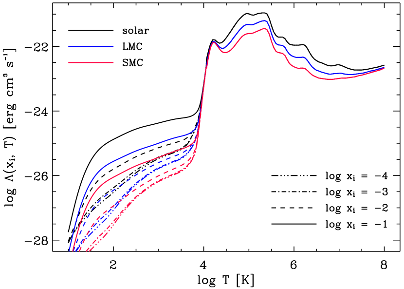
Figure 1.— Composite cooling curve (see text) for various ionization degrees and for metallicities corresponding to the solar neighborhood, the LMC and the SMC.

2.2. Gravity, Jeans Instability (GI)

A (one-dimensional) region becomes gravitationally unstable if

$$\rho>\frac{(c_{s}\,k)^{2}}{4\pi G},$$ (6)

with the wave number $k$ and mass density $\rho\equiv\mu n$. The corresponding time scale is

$$\tau_{GI}=(4\pi G\rho-c_{s}^{2}k^{2})^{-1/2},$$ (7)

again including the condition for instability. Gravitational collapse occurs for $\tau_{GI}\in\mathbb{R}$.

2.3. Non-Linear Thin Shell Instability (NTSI)

The NTSI (Vishniac, 1994) arises in a shock-bounded slab, when ripples in a two-dimensional slab focus incoming shocked material and produce density fluctuations. The growth rate of the NTSI is mostly controlled by $k\eta$, the product of the wave number of the slab perturbation $k=2\pi/L$, and the amplitude of the slab’s initial displacement $\eta$ (equivalently, the amplitude of the collision interface’s geometrical perturbation). The instability is driven by lateral transport of longitudinal momentum, i.e. if the inflow is parallel to the $x$ direction, and the slab is in the $y$-$z$-plane, $x$-momentum is transported laterally in $y$ (and $z$), collecting at the focal points of the perturbed slab. The efficiency of lateral momentum transport is key to the development of the instability, since it is the imbalance of ram pressure at the focal points that eventually propels matter forward, driving the growth of the slab’s perturbation. Vishniac (1994) derived a growth timescale of

$$\tau_{NTSI}\approx[c_{s}k(k\eta)^{1/2}]^{-1}.$$ (8)

Blondin & Marks (1996) found that at constant $\eta$ and for small $k$, equation (8) yields only a lower limit, while for large $k$, the analytical growth rates agree well with the numerical results. The reason for this seems to lie in the efficiency of deflecting the incoming flow: for small $k$, a small fraction of the incoming flow’s momentum is converted to lateral motions, while a large part compresses the slab (depending on the equation of state, this could lead to an increase in energy losses). For the parameter study (§3), we set $\eta\equiv L/4$. Keeping $k$ constant and varying $\eta$ affects the NTSI in a similar way as keeping $\eta$ constant and changing $k$, with a weaker dependence on $\eta$. Magnetic fields can suppress the NTSI if the ram pressure of the incoming flow drops below the magnetic pressure (Heitsch et al., 2007). The NTSI is an efficient dynamical focusing mechanism for large-scale gas streams, resulting in the rapid build-up of massive cores in the focal points (Hueckstaedt, 2003) as possible sites for massive star formation (Heitsch et al., 2008).

2.4. Kelvin-Helmholtz-Instability (KHI)

The NTSI converts the highly compressible modes of the inflows into shear flows at the flanks of the perturbed slab. These shear flows give rise to the KHI, which thus is secondary to the NTSI, but which also is the main turbulence generation mechanism. The turbulence in turn leads to the saturation of the NTSI (Vishniac, 1994). In the simplest – incompressible – scenario of the KHI (Chandrasekhar, 1961), the shear layer has constant density, and the velocity profile is a step function. In this case, the growth timescale is given by the velocity difference $\Delta U$ and the wave number as

$$\tau_{KHI}=(k\Delta U)^{-1},$$ (9)

i.e. the system is unconditionally unstable. This is definitely the most extreme case: magnetic field components parallel to the shear flows can stabilize against the KHI, and for compressible flows, the system will be stable for all those wave numbers whose effective Mach number is larger than a critical value (Gerwin, 1968). For a detailed discussion of the KHI, see Palotti et al. (2008).

2.5. Other Instabilities

The list of instabilities and their effects considered here is by no means exhaustive. For instance, Inoue et al. (2006) discuss a corrugation instability of evaporation fronts appearing at the interface between the WNM and the CNM on timescales of approximately $\sim 1$ Myr in the WNM, and down to $0.01$ Myr in the CNM. This – so they argue – is on the order of the cooling timescales in each of the media, so that the instability could contribute to the generation of turbulence in the ISM. Hence the corrugation instability will play an important role for the dynamics of the WNM/CNM. However, as equation (47) and Figure 9 of Inoue et al. (2006) demonstrate, the growth timescale of the corrugation instability is in the (for our application) interesting range of $\lesssim 1Myr$ only for sub-parsec scales, which are substantially smaller than the large-scale flows sweeping up whole clouds as envisaged in the current study.

In a similar vein, we do not discuss turbulence generation by the TI alone. This possibility has been investigated extensively (e.g. Burkert & Lin, 2000; Kritsuk & Norman, 2002b; Vázquez-Semadeni et al., 2003). Cox (2005) points out that because of the limited energy reservoir, thermal pressure variations in a bistable ISM are expected to have negligible dynamical effects, requiring additional sources or triggers for turbulence generation (e.g. Kritsuk & Norman, 2002a).

2.6. Criteria for Instability Dominance

The characteristic timescales (eqs. [5,7,8,9]) can be used to derive criteria for the dominance of a given instability in terms of physical quantities. We chose (particle) density and temperature, to facilitate a straight-forward comparison to ISM regimes. Attributes in square brackets in each of the following subsection titles stand for the line-styles used in Figure 2. Not all combinations are physically relevant. For instance, $\tau_{c}\ll\tau_{GI}$ generally for gravitationally unstable regimes (§3.2). The ratio of specific heat capacities is set to $\gamma\equiv 5/3$, and the mean molecular weight $\equiv 2.36$. Obviously, these choices are not valid over the full parameter range discussed, but they will considerably simplify the discussion.

2.6.1 Gravity threshold [green dashed]

A region will be gravitationally unstable if

$$n > \frac{\gamma k_{B}}{4\pi G\mu^{2}}\,k^{2}\,T$$

$$\approx 7.4\times 10^{1}\frac{T}{[\mbox{K}]}\,\left(\frac{L}{[\mbox{pc}]}\right)^{2}\,\mbox{cm}^{-3}..$$

This is just equation (6) expressed in terms of temperature.

2.6.2 GI dominates NTSI and KHI [red dashed]

If condition (2.6.1) is fulfilled, gravitation will dominate the NTSI if

$$n > \frac{\gamma\,k_{B}}{4\pi G\mu^{2}}\,k^{3}\,\eta\,T$$

$$\approx 4.7\times 10^{2}\frac{\eta}{[\mbox{pc}]}\,\left(\frac{L}{[\mbox{pc}]}\right)^{-3}\,\frac{T}{[\mbox{K}]}\,\mbox{cm}^{-3},$$

where $\eta$ is the displacement of the slab. Note the strong dependence on the wave number $k$, which hints at the power of dynamical fragmentation to prevent global gravitational collapse.

The condition for the KHI is similar to conditions (2.6.1) and (2.6.2). The GI dominates over the KHI for

$$n > \frac{\gamma\,k_{B}}{4\pi G\mu^{2}}\,{\cal M}\,k^{2}\,T$$

$$\approx 7.4\times 10^{1}{\cal M}\,\frac{T}{[\mbox{K}]}\,\left(\frac{L}{[\mbox{pc}]}\right)^{-2}\,\mbox{cm}^{-3},$$

where ${\cal M}$ is the Mach number of the shear flow. This is the most beneficial case for the KHI: for supersonic flows, the KHI is not unconditionally unstable anymore.

Since conditions (2.6.2) and (2.6.2) each depend linearly on the temperature, they will behave similarly in the $(n,T)$, plane. Without loss of generality, we can combine them in §3.

2.6.3 TI dominates NTSI and KHI [red solid]

The TI dominates the NTSI for

$$n > \left(\frac{\gamma}{\mu}\right)^{1/2}\,k^{3/2}\,\eta^{1/2}\,\frac{(k_{B}T)^{3/2}}{\Lambda(T)}$$

$$\approx 5.4\times 10^{-4}\left(\frac{\eta}{[\mbox{pc}]}\right)^{1/2}\left(\frac{L}{[\mbox{pc}]}\right)^{-3/2}\left(\frac{T}{[\mbox{K}]}\right)^{3/2}$$

$$\times \left(\frac{10^{26}\Lambda(T)}{[\mbox{erg cm${}^{3}$ s${}^{-1}$}]}\right)^{-1}\,\mbox{cm}^{-3}.$$

This just mirrors the fact that with increasing density the cooling becomes stronger. A similar condition can be derived for the KHI by replacing $(k\eta)^{1/2}$ by the velocity difference multiplied by the wave number.

2.6.4 Sound crossing time limit for the TI [blue solid]

As discussed in §2.1, we use the sound crossing scale (eq. 1) for the TI’s condensation mode as a proxy to estimate the importance of the TI. It leads to a density threshold above which the condensation mode of the TI cannot be excited:

$$n < \left(\frac{\gamma}{\mu}\right)^{1/2}\,k\,\frac{(k_{B}T)^{3/2}}{\Lambda(T)}$$

$$\approx 2.2\times 10^{-4}\left(\frac{L}{[\mbox{pc}]}\right)^{-1}\left(\frac{T}{[\mbox{K}]}\right)^{3/2}\left(\frac{10^{26}\Lambda(T)}{[\mbox{erg cm${}^{3}$ s${}^{-1}$}]}\right)^{-1}.$$

The smaller the scales, the less restrictive is the limit on the density for the condensation mode. The temperature dependence is given by the detailed form of the cooling curve.

3. Discussion

The conditions summarized in §2.6 allow us to identify the dominant instabilities in the two-dimensional $(n,T)$ parameter plane. Most of the conditions (2.6.1)-(2.6.4) depend on the spatial scale. Figure 2 summarizes the regimes in four diagrams, at characteristic (fixed) scales of $0.1,1.0,10$ and $10^{2}$ pc. Table 1 provides a key to the line styles and colors used in Figure 2. We will discuss the dominant instabilities (§3.1–3.4) and an evolutionary sequence of a fluid parcel in the ISM (§3.5).

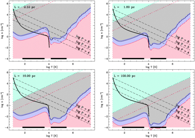
Figure 2.— Summary of the instability regimes in $(n,T)$-space, for four characteristic spatial scales as indicated in the top left corners. The diagonal black long-dashed lines denote lines of constant pressure as indicated. The thick black line between $1<\log T<4$ represents the thermal equilibrium curve due to a balance between heating and cooling. The horizontal thick black lines at the bottom of each panel denote the ranges of the two thermally unstable regimes. Fragmentation by cooling dominates in all regions with right-slanted hashing (red, blue and black), while gravity dominates fragmentation in the left-slanted hashed region (green). Red stands for dominance of dynamical instabilities over cooling/TI. Blue/black indicates where fragmentation by cooling dominates. The blue ribbon and the black horizontal lines together indicate ranges of strict thermal instability. See Table 1 for a summary of the line styles and colors.

Table 1Key to Figure 2

line style	meaning	equation
hashed, slanted right	fragmentation by cooling or TI
hashed, slanted left	fragmentation by gravity
red hashed	dynamics dominate cooling
blue hashed	cooling/TI dominates dynamics
black hashed	cooling (but not TI) dominates dynamics
green dash	Jeans criterion	(2.6.1)
red dash	GI dominates NTSI	(2.6.2)
red solid	TI dominates NTSI	(2.6.3)
blue solid	TI crossing time	(2.6.4)

3.1. Thermally Dominated Regime

The most prominent feature in Figure 2 is the large extent of the thermally dominated parameter regime (right-slanted hashing; blue and black). This regime is limited by the growing importance of dynamical instabilities (red) towards low densities, and by the Jeans condition (eq. 2.6.1) towards high densities. Towards low densities (red), the thermal timescales get longer than the dynamical timescales, so that the gas will tend to behave adiabatically. Within the blue hashed region, cooling dominates dynamical instabilities, leading to the TI within the temperature ranges indicated by the thick black horizontal bars. Outside the strictly thermally unstable regions, cooling still dominates and can lead to fragmentation when an external (ram or gravitational) pressure is applied. Thus, while the TI dominates the dynamics only within certain temperature ranges, thermal effects (strong cooling) continue to dominate all through the black hashed region at higher densities. The upper edge of the blue ribbon is determined by the sound crossing time condition (2.6.4), which is – strictly – only applicable to the TI. There are two thermally unstable regimes (according to eq. [4]): The lower one between $10^{2}<T<10^{4}$ K connects the warm and cold neutral medium (WNM and CNM), while the upper (of lesser strength) in the range of $T\approx 10^{5}$ connects the hot and warm ionized medium (HIM and WIM).

The curved thick black line between $10<T<10^{4}$ K denotes the thermal equilibrium curve, where heating terms balance cooling terms. At $T\approx 10^{4}$ K and $n<1$ cm^-3, the ISM behaves quasi-isothermal. The signature of the thermal instability is a pressure loss with increasing density (compare to dashed lines of constant pressure). Moving to high densities and lower temperatures, the effective equation of state tends back to isothermality but stays sub-isothermal, i.e. $\gamma_{eff}<1$. The thermal equilibrium curve is describing an approximate evolutionary sequence of a fluid element from the WNM to the CNM (see §3.5).

Before we compare the relative strengths of the instabilities, Figure 3 offers a more detailed view of the TI in the WNM. As orientation and for comparison with Figure 2, the lines of constant pressure and the sound crossing time limit (eq. [2.6.4]) for the TI have been indicated in the same style as in Figure 2. The color-shaded region denotes the growth timescale (eq. [5]) of the TI (see color bar to the right of the diagrams) in all locations where the TI can be excited. There are two points to notice here:

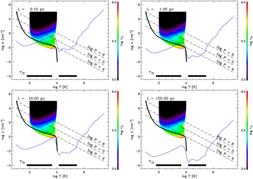
Figure 3.— A more detailed look at the TI in $(n,T)$-space, for four characteristic spatial scales as indicated in the top left corners. The diagonal black long-dashed lines denote lines of constant pressure as indicated. The thick black line between $1<\log T<4$ represents the thermal equilibrium curve due to a balance between heating and cooling. The horizontal thick black lines at the bottom of each panel denote the ranges of the two thermally unstable regimes. The blue line denotes the maximum density given by the sound crossing time limit (eq. [2.6.4]). The color-shaded region shows the growth timescale of the TI (eq. [5]). Light green corresponds to a timescale of $\approx 1$ Myr.

(1) Looking at the upper left panel ($L=0.1$ pc), the timescale $\tau_{TI}$ can become extremely short; however, around the thermally unstable region, it is on the order of $1$ Myr (light green, traced by the thermal equilibrium curve), comparable to dynamical timescales. This leads to a noticeable amount of thermally unstable gas (e.g. Heiles & Troland, 2003 for observations of neutral hydrogen, and Gazol et al., 2001, Sánchez-Salcedo et al., 2002, Audit & Hennebelle, 2005, Heitsch et al., 2006 for evidence from numerical models). For the isothermal branch at $T\approx 10^{4}$ K, the TI is essentially absent. Thus, the lower the density on the (warm) isothermal branch, the higher the compression due to e.g. shocks needs to be to trigger the TI. Since the post-shock density in an isothermal gas scales with the square of the Mach number, this condition is not overly restrictive.

(2) With increasing spatial scale (solid blue line in the remaining three panels of Fig. 3), the upper density limit for the TI drops due to the sound crossing time condition (2.6.4). Strictly, the TI will only be excited if there is a color-shaded region below the blue line, so to speak. This leaves us with the somewhat puzzling result that for scales $L>10$ pc, the TI seemingly cannot be excited. The solution is two-fold: (a) At large scales (and lower densities/higher temperatures), the upper TI at $10^{5}$ K kicks in, and (b) the notion of fixed scales is misleading. The TI will be triggered by compressions and/or turbulent mixing equivalent to a reduction of spatial scale. Moreover, since it is a condensation mode, we cannot regard the evolution of the TI at a fixed scale, but need to follow a fluid parcel (see §3.5).

3.2. Gravitation against Thermal Instability

The Jeans criterion (eq. [2.6.1]) is fulfilled for all pairs $(n,T)$ above the green dashed line in Figure 2 – e.g., for densities $n>10^{5}$ cm^-3 and temperatures $T\approx 10$ K at $0.1$ pc. With increasing scale, the $(n,T)$-regime dominated by gravitation extends more and more to lower densities and higher temperatures. At large scales ($\approx 10$ pc), gravity starts to dominate the parameter space, indicating the importance of global gravitational modes.

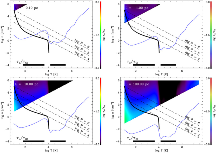
Figure 4.— Comparison of characteristic times for self-gravity and cooling in $(n,T)$-space, for four characteristic spatial scales as indicated in the top left corners. The diagonal black long-dashed lines denote lines of constant pressure as indicated. The thick black line between $1<\log T<4$ represents the thermal equilibrium curve due to a balance between heating and cooling. The horizontal thick black lines at the bottom of each panel denote the ranges of the two thermally unstable regimes. The blue line denotes the maximum density given by the sound crossing time limit (eq. [2.6.4]). The color-shaded triangles show the ratio $\tau_{c}/\tau_{GI}$ (eqs. [2], [7]) for the pairs of $(n,T)$ subject to the GI. Yellow would correspond to $\tau_{c}=\tau_{GI}$ – obviously, $\tau_{c}<\tau_{GI}$ for all gravitationally dominated pairs of $(n,T)$.

Figure 4 compares the relative strengths of gravitational over thermal condensation. Shown are the same plots as in the previous figures, but now overlaid with the ratio $\tau_{c}/\tau_{GI}$ for the gravitationally dominated $(n,T)$-regime (eq. 7). Yellow (see color bar of $\tau_{c}/\tau_{GI}$) denotes $\tau_{c}=\tau_{GI}$. The cooling timescales are substantially shorter than any gravitational timescales over the whole parameter range accessible to the GI. If the TI can be excited (e.g between $80<T<5000$ K), this means that thermal condensations will be the dominant fragmentation process. For parameters $(n,T)$ not subjected to the TI, the short cooling timescales mean only that any excess energy due to compressions (by gravity!) will be efficiently radiated away.

3.3. Gravitational against dynamical effects

The relative importance of gravity and dynamics can be read off equations (2.6.1)–(2.6.2). The discerning line for GI against NTSI is shown in Figure 2 as a red dashed line – obviously, the NTSI ceases to be important before densities high enough for gravitational collapse can be reached. Equations (2.6.1) and (2.6.2) on the other hand show that for Mach numbers ${\cal M}>1$, the KHI can still dominate in gravitationally unstable gas. This is the regime of turbulent fragmentation in a Jeans-unstable medium discussed in detail by Mac Low & Klessen (2004).

3.4. Thermal against dynamical effects

Dynamical instabilities dominate below the red (NTSI) and the black (KHI) lines (Fig. 2), generally however in the red hashed region. They impose a lower density threshold on the importance of cooling (and of the TI within the applicable temperature range), i.e. the gas will tend to behave more and more adiabatically for those regions in $(n,T)$-space.

Figure 5 shows the ratio of the cooling time scale (eq. [2]) over $\tau_{NTSI}$ (eq. [2.6.3]), where the latter is used as a proxy of dynamical instabilities. Since the cooling timescale does not depend on the spatial scale, dynamical instabilities can become dominant for small scales ($L=0.1\cdots 1.0$ pc) in the WNM ($T\approx 10^{4}$ K). With increasing density, cooling dominates dynamics, but the TI is still limited by condition (2.6.4).

Dynamical instabilities entail the generation of turbulence – especially at the high Reynolds numbers in the ISM. The turbulent cascade leads to a spectrum of density perturbations, populating a wide range of spatial scales. In other words: instead of proceeding at a fixed scale, the TI will act on all density perturbations within its parameter range (see Fig. 3) at scales smaller than the sound crossing scale simultaneously.

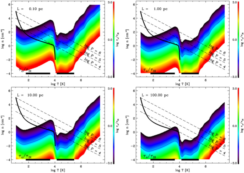
Figure 5.— Comparison of characteristic times for dynamical instabilities and cooling in $(n,T)$-space, for four characteristic spatial scales as indicated in the top left corners. The diagonal black long-dashed lines denote lines of constant pressure as indicated. The thick black line between $1<\log T<4$ represents the thermal equilibrium curve due to a balance between heating and cooling. The horizontal thick black lines at the bottom of each panel denote the ranges of the two thermally unstable regimes. The blue line denotes the maximum density given by the sound crossing time limit (eq. [2.6.4]). The color-shaded regions show the ratio $\tau_{c}/\tau_{DI}$ (eqs. [2], [2.6.3]). Note that the ratio decreases monotonically with increasing density.

3.5. An Evolutionary Sequence

The strength and importance of the TI is based on the one hand on the fact that it grows on the smallest scales first (Burkert & Lin, 2000) and thus can feed on ubiquitous small-scale structures generated by turbulence. On the other hand, the condensation mode of the TI does not proceed at a fixed scale: a fluid parcel which gets thermally unstable will contract to smaller scales and thus “delay” running into the sound crossing scale condition (2.6.4).

To see this, consider the thermal equilibrium curve (solid black curve in e.g. Figs. 2 and 3). Numerical simulations of the fragmentation of shocked flows in a thermally unstable medium demonstrate that the gas generally follows this thermal equilibrium curve (see Fig. 3 of Audit & Hennebelle, 2005, and Fig. 14 of Heitsch et al., 2006), so that it can be interpreted as an evolutionary sequence from the WNM to the CNM. While the equilibrium curve is well defined at the high-density end due to extremely short cooling time scales (see Fig. 3), the scatter especially in the thermally unstable regime can be substantial and depends largely on the ratio between the dynamical and the cooling timescales (Figs. 14 and 15 of Heitsch et al., 2006).

A fluid parcel in the WNM/WIM starts out at a scale of e.g. $\sim 1$ pc and a density of a little under $1$ cm^-3. The parcel may be compressed due to a shock wave, or turbulence may lead to density variations. In any case, the density increases, propelling the parcel upwards along the isothermal branch of the equilibrium curve, reducing the cooling timescales (Fig. 3) and thus eventually lowering the temperature. The fluid parcel will follow (approximately) the equilibrium curve along its sharp left-turn into the thermally unstable regime. Looking at the 1 pc panel, by then, the fluid parcel will have left the region of thermal instability (Fig. 2). However, the compression above not only increased the density, but also reduced the scale, so that effectively the thermally unstable regime (blue hashed) shifts upwards to higher densities, moving us from the $1$ pc panel to the $0.1$ pc panel in Figures 2 or 3.

Once the fluid parcel has entered the thermally unstable regime, it evolves (more or less) along lines of constant pressure towards higher densities and lower temperatures. In the condensation mode, this is equivalent to a further shrinking of the fluid parcel’s volume, so that the blue ribbon of thermal instability essentially “moves” to smaller scales with the fluid parcel on its way along the equilibrium curve. This “co-moving” or Lagrangian behavior is crucial for the strength and the importance of the condensation mode of the TI in the ISM.

Yet the above statement calls for a caveat. A closer inspection of equation (2.6.4) reveals the following. Assuming that the fluid parcel evolves under constant pressure $P_{0}$ – actually, for dynamical times substantially longer than thermal timescales, the fluid parcel will follow approximately the thermal equilibrium curve (Sánchez-Salcedo et al., 2002; and Fig. 2), which is sub-isobaric as indicated by $\gamma_{eff}<0$ in the thermally unstable regime – and with a constant cooling strength $\Lambda_{0}$, the sound crossing scale condition (2.6.4) translates into an expression for the outer length scale $L_{T}$ of thermal instability,

$$L_{T}<a_{0}\,n^{-5/2},$$ (15)

equivalent to equation (1), with the constant

$$a_{0}\equiv 2\pi\,\left(\frac{\gamma\,k_{B}}{\mu}\right)^{1/2}\,\frac{P_{0}^{3/2}}{\Lambda_{0}}.$$ (16)

A spherical blob of constant mass $m_{0}$ will contract as

$$L_{V}=b_{0}\,n^{-1/3},$$ (17)

with the constant

$$b_{0}\equiv\left(\frac{6\,m_{0}}{\pi\,\mu}\right)^{1/3}.$$ (18)

Thus,

$$L_{T}\propto L_{V}\,n^{-13/6},$$ (19)

meaning that the sound crossing scale (eq. [1]) shrinks more rapidly by a factor of $\approx n^{2}$ than the size of the fluid parcel. Even a one-dimensional compression $L_{V}\propto n^{-1}$ would still result in $L_{T}\propto L_{V}\,n^{-3/2}$. This would move the fluid parcel out of the thermally unstable regime. If the fluid parcel contracts “faster” than the sound crossing time criterion allows, the condensation mode will be suppressed, but the isochoric mode of the TI still will be excited. This is specifically the case for the black hashed regions (Fig. 2) where thermal timescales are substantially shorter than the dynamical timescales. The thermal pressure of the fluid parcel can then drop below that of the surrounding medium, and the resulting waves will lead to further fragmentation (smaller scales) and compression, triggering again the condensation mode. In that sense, while the co-moving picture is a simplification, the more realistic evolution of a fluid parcel involving isobaric and isochoric modes will lead to even more fragmentation.

Eventually, our fluid parcel will reach the sub-isothermal branch of the thermal equilibrium curve below $\approx 80$ K, entering the gravitationally dominated regime (as discussed earlier, this regime is characterized also by extremely short cooling timescales). In the presence of an “external” pressure (due to e.g. gravity), the sub-isothermal equation of state can lead to further fragmentation.

However, gravity will not only play a local role. At large scales, global gravity can be dominant (Fig. 2, e.g. 10 pc). Global gravitational modes in combination with a finite extent of the cloud can easily lead to the sweep-up of material at the edges of the cloud (Burkert & Hartmann, 2004; see Vázquez-Semadeni et al., 2007 and Heitsch et al., 2008 for numerical evidence). Due to the rapid evolution of the local (thermal and dynamical) instabilities, the resulting filaments will have substructure, leading to further fragmentation into cores.

The thermal instability thus offers a short-cut to reach the gravitationally dominated regime from the warm, isothermal branch (at $T=10^{4}$ K). Instead of having to compress the gas isothermally by a factor of $\approx 10^{4}$ – corresponding to a Mach number of $10^{2}$ – only a modest compression is needed in the warm isothermal branch to move the fluid parcel up the thermally stable equilibrium line and “push it over the ledge”. This allows star formation in environments without high pressurization and/or deep gravitational potentials.

To summarize, the generation of turbulence due to dynamical instabilities (red hashed regime) introduces density variations at smaller scales, triggering the thermal instability, which in turn amplifies the density perturbations. The growth of the thermal instability is eventually limited by the mass reservoir available, and thus by the external pressure (Kritsuk & Norman, 2002b, a). This could take the form of global gravity, cloud collisions, expanding shells or galaxy mergers. Gravity acts locally on the high-density seeds, allowing rapid collapse before edge effects of global gravity (Burkert & Hartmann, 2004) overrun the local perturbations.

3.6. Limitations

Obvious limitations of the study include neglecting the effect of structure in the inflows, a generic cooling curve, the missing time-dependence and neglecting magnetic fields. Each of these is discussed in turn below.

3.6.1 The Structure-less Inflows

Our analysis approaches the problem of structured cloud formation from the angle of a “worst case” scenario, using the most unfavorable initial conditions to generate turbulence and substructure, by considering (as in our numerical work) the large-scale flows to be uniform. Obviously – as pointed out earlier (Heitsch et al., 2006) – this assumption neglects the possibility that the flows themselves already might contain substructure. This however is not problematic, as our goal is to demonstrate that substructure can arise from uniform flows with only small, long-wavelength initial perturbations. The introduction of structure in the inflows – specifically a mixture of WNM/CNM instead of just WNM – would make it even easier to form substructure. Moreover, introducing substructure in the inflows raises the question of just what form should be assumed. The most common initial conditions for numerical simulations of cloud formation comprise density perturbations (e.g. Inutsuka et al., 2005), velocity “noise” (e.g. Vázquez-Semadeni et al., 2007), or a turbulent velocity distribution (e.g. Hennebelle et al., 2007), but the theoretical justification of these assumptions is unclear. Moreover, it is far from obvious that driving mechanisms such as that of a spherical stellar wind, H II region expansion, or supernova bubble expansion are highly turbulent and structured in the absence of interaction with the surrounding medium. By ignoring substructure in the inflows we can consider the most general (and unfavorable) cases for generating turbulent substructure.

3.6.2 Cooling Curve

Our cooling curve at low temperatures is mainly limited by the fact that it does not include molecular line cooling or the formation of molecules. Molecular cooling would lower the cooling timescales further, driving the cooling curve more to isothermality. The formation of H₂ lowers the sound speed by a factor of $\sqrt{2}$ and the pressure by $2$, thus introducing an additional pressure loss at high densities. While the thermal equilibrium curve will describe the evolution of a fluid parcel approximately correctly from the WNM to the CNM, the details of the evolution at high densities and low temperature are less realistic.

The heating and cooling functions $\Gamma$ and $\Lambda$ were defined for solar abundances and a Galactic UV background. Reducing the metallicity by e.g. a factor of $10$ to values typical for the SMC reduces the cooling strength below $T\approx 10^{4}$ K by approximately the same factor (see Fig. 1). Thus, the blue ribbon in Figure 2 would move up to higher densities.

3.6.3 Time dependence

Obviously, the analysis does not include any time evolution (although a rough idea of the dynamical evolution can be gleaned from following the thermal equilibrium curve connecting the WNM and CNM, §3.5). Dynamical effects (turbulence, shocks) are expected to render thermal effects (cooling, TI) even stronger, specifically by providing small-scale seeds, and by allowing the TI to act on many scales simultaneously. This can clearly be seen in the high-resolution two-dimensional simulations by Hennebelle et al. (2007) and Hennebelle & Audit (2007). For a detailed discussion of (fully developed) turbulence in combination with the TI, see e.g. Vázquez-Semadeni et al. (2003) and Audit & Hennebelle (2005). The latter authors point out that increasing the level of turbulence will lower the CNM fraction, an effect depending on the ratio of dynamical over thermal timescales (see also Heitsch et al., 2006).

Certain simplifications had to be made, e.g. the Mach number for the KHI (eq. 9) was set to $1$. While this is a good approximation for many regimes in the ISM that exhibit trans-sonic flows, it will fail in cases of extreme shear flow conditions such as HVCs or molecular clouds (however, see Fig. 9 of Heitsch et al., 2006).

3.6.4 Magnetic Fields

Magnetic fields are not included. In relevance to the flow-driven cloud formation scenario, they would introduce a threshold criterion for the KHI (Chandrasekhar, 1961) and the NTSI (Heitsch et al., 2007), and they may affect the evolution of the TI (Field, 1965). Critical field strengths and angles for the suppression of the condensation mode in one-dimensional converging flows have been identified by (Hennebelle & Pérault, 2000). Two-dimensional models of flow-driven cloud formation with the magnetic field perpendicular to the inflows (Inoue & Inutsuka, 2008) demonstrate that while the fields can suppress the formation of high-density clouds, thermal fragmentation still occurs, leading to highly filamentary cold HI clouds. These results lighten somewhat the restrictive low limits on the perpendicular field strengths derived from one-dimensional arguments (Bergin et al., 2004). On a larger (galactic spiral arm) scale, numerical models by Kim et al. (2003) and Kim & Ostriker (2006) demonstrate the importance of magnetic fields for channeling gas streams.

4. Summary

To form stars, molecular clouds need to fragment on scales vastly smaller than their overall dimensions. Self-gravity in combination with supersonic turbulence allows the rapid fragmentation of Jeans-unstable regions (Larson, 1981; Elmegreen, 1993; Mac Low & Klessen, 2004). Yet unless the density perturbations in molecular clouds are non-linear before the onset of global gravitational collapse, global gravity tends to win and “overrun” any local perturbation (Burkert & Hartmann, 2004). Thus, a strong fragmentation mechanism is needed during the formation of the cloud to provide simultaneously the observed turbulence as well as the initial density seeds for the rapid local gravitational collapse mandated by the observed rapid onset of star formation (Hartmann et al., 2001; Hartmann, 2002).

The flow-driven formation of molecular clouds in large-scale flows of atomic hydrogen provides a natural fragmentation mechanism due to a combination of dynamical and strong thermal instabilities (see references in §1). As demonstrated by numerical models, this fragmentation mechanism does not need to recur on imposed turbulent velocity fields, but arises from the physical conditions in the WNM/CNM. The rapid fragmentation of the shocked flows will form high-density seeds for local gravity to take over, while gravitational forces on the cloud scale can sweep up material into filaments (Heitsch et al., 2008).

The above outline of the connection between cloud formation and the initial conditions for star formation mainly rests on evidence from numerical simulations. In the present study we discussed the timescales of the instabilities dominating the evolution of shocked flows. Guided by our earlier work, we identify four instabilities, namely two condensation mechanisms (gravity and thermal instability) and two fluid instabilities (NTSI and KHI). We determine the parameter regime in density, temperature and scale in which each of the instabilities is expected to dominate. These are our findings and their implications:

1. The (dynamical and thermal) instabilities leading to the rapid fragmentation of shocked flows dominate on small scales for reasonable parameters of the WNM and CNM (Fig. 2).

2. Cooling timescales (of $\approx 1$ Myr in the thermally unstable regime) are generally substantially shorter than gravitational timescales for that same density and temperature regime (Fig. 4). Thus, thermal fragmentation dominates gravitational fragmentation during cloud formation.

3. The strength of the condensation mode of the TI derives from two effects, namely that it grows on the smallest scales first, and that it is essentially a co-moving (or Lagrangian) mode, i.e. the unstable region shrinks, thus keeping “longer” below the sound crossing scale $\lambda_{c}$ (eq. [2.6.4]). Feeding on turbulent density perturbations below $\lambda_{c}$ will allow the TI to grow on many scales simultaneously.

4. The preference of small scales by the TI entails the preference to form sheets and filaments: the shorter axes are more susceptible to become unstable. This is an obvious parallel to the GI, with the – equally obvious but crucial – difference that the GI will act globally and locally.

5. The fragmentation due to thermal effects is crucial for the formation of small-scale, high-density perturbations during the formation of the molecular cloud, to provide the seeds for rapid local gravitational collapse before global gravity dominates the dynamics completely.

6. The all-important role of the TI due to the intermittent nature of the turbulence driven by dynamical instabilities allows an early fragmentation of the converging flows, before (local) gravity can take over. This supports numerical findings that the (molecular) core mass spectrum might be set to some extent (Dib et al., 2008) early on during cloud formation by thermal fragmentation (Hennebelle et al., 2007; Heitsch et al., 2008).

References

- Audit & Hennebelle (2005) Audit, E. & Hennebelle, P. 2005, A&A, 433, 1
- Balbus (1995) Balbus, S. A. 1995, in Astronomical Society of the Pacific Conference Series, Vol. 80, The Physics of the Interstellar Medium and Intergalactic Medium, ed. A. Ferrara, C. F. McKee, C. Heiles, & P. R. Shapiro, 328
- Ballesteros-Paredes & Hartmann (2007) Ballesteros-Paredes, J. & Hartmann, L. 2007, Revista Mexicana de Astronomia y Astrofisica, 43, 123
- Ballesteros-Paredes et al. (1999) Ballesteros-Paredes, J., Vázquez-Semadeni, E., & Scalo, J. 1999, ApJ, 515, 286
- Bergin et al. (2004) Bergin, E. A., Hartmann, L. W., Raymond, J. C., & Ballesteros-Paredes, J. 2004, ApJ, 612, 921
- Blondin & Marks (1996) Blondin, J. M. & Marks, B. S. 1996, New Astronomy, 1, 235
- Burkert & Hartmann (2004) Burkert, A. & Hartmann, L. 2004, ApJ, 616, 288
- Burkert & Lin (2000) Burkert, A. & Lin, D. N. C. 2000, ApJ, 537, 270
- Chandrasekhar (1961) Chandrasekhar, S. 1961, Hydrodynamic and hydromagnetic stability (International Series of Monographs on Physics, Oxford: Clarendon, 1961)
- Cox (2005) Cox, D. P. 2005, ARA&A, 43, 337
- Dalgarno & McCray (1972) Dalgarno, A. & McCray, R. A. 1972, ARA&A, 10, 375
- Dib et al. (2008) Dib, S., Brandenburg, A., Kim, J., Gopinathan, M., & Andre, P. 2008, ArXiv e-prints, 801
- Dobbs & Bonnell (2007) Dobbs, C. L. & Bonnell, I. A. 2007, MNRAS, 376, 1747
- Dobbs & Bonnell (2008) —. 2008, MNRAS, 285
- Elmegreen (1993) Elmegreen, B. G. 1993, ApJ, 419, L29+
- Elmegreen (2007) —. 2007, ApJ, 668, 1064
- Elmegreen & Lada (1977) Elmegreen, B. G. & Lada, C. J. 1977, ApJ, 214, 725
- Field (1965) Field, G. B. 1965, ApJ, 142, 531
- Garnett (1999) Garnett, D. R. 1999, in IAU Symposium, Vol. 190, New Views of the Magellanic Clouds, ed. Y.-H. Chu, N. Suntzeff, J. Hesser, & D. Bohlender, 266–272
- Gazol et al. (2001) Gazol, A., Vázquez-Semadeni, E., Sánchez-Salcedo, F. J., & Scalo, J. 2001, ApJ, 557, L121
- Gerwin (1968) Gerwin, R. A. 1968, Reviews of Modern Physics, 40, 652
- Hartmann (2002) Hartmann, L. 2002, ApJ, 578, 914
- Hartmann et al. (2001) Hartmann, L., Ballesteros-Paredes, J., & Bergin, E. A. 2001, ApJ, 562, 852
- Hartmann & Burkert (2007) Hartmann, L. & Burkert, A. 2007, ApJ, 654, 988
- Heiles & Troland (2003) Heiles, C. & Troland, T. H. 2003, ApJ, 586, 1067
- Heitsch et al. (2005) Heitsch, F., Burkert, A., Hartmann, L. W., Slyz, A. D., & Devriendt, J. E. G. 2005, ApJ, 633, L113
- Heitsch et al. (2008) Heitsch, F., Hartmann, L. W., Slyz, A. D., Devriendt, J. E. G., & Burkert, A. 2008, ApJ, 674, 316
- Heitsch et al. (2006) Heitsch, F., Slyz, A. D., Devriendt, J. E. G., Hartmann, L. W., & Burkert, A. 2006, ApJ, 648, 1052
- Heitsch et al. (2007) —. 2007, ApJ, 665, 445
- Hennebelle & Audit (2007) Hennebelle, P. & Audit, E. 2007, A&A, 465, 431
- Hennebelle et al. (2007) Hennebelle, P., Audit, E., & Miville-Deschênes, M.-A. 2007, A&A, 465, 445
- Hennebelle & Pérault (1999) Hennebelle, P. & Pérault, M. 1999, A&A, 351, 309
- Hennebelle & Pérault (2000) —. 2000, A&A, 359, 1124
- Hueckstaedt (2003) Hueckstaedt, R. M. 2003, New Astronomy, 8, 295
- Inoue & Inutsuka (2008) Inoue, T. & Inutsuka, S.-i. 2008, ArXiv e-prints, 801
- Inoue et al. (2006) Inoue, T., Inutsuka, S.-i., & Koyama, H. 2006, ApJ, 652, 1331
- Inutsuka et al. (2005) Inutsuka, S.-I., Koyama, H., & Inoue, T. 2005, in American Institute of Physics Conference Series, Vol. 784, Magnetic Fields in the Universe: From Laboratory and Stars to Primordial Structures., ed. E. M. de Gouveia dal Pino, G. Lugones, & A. Lazarian, 318–328
- Kim & Ostriker (2006) Kim, W.-T. & Ostriker, E. C. 2006, ApJ, 646, 213
- Kim et al. (2003) Kim, W.-T., Ostriker, E. C., & Stone, J. M. 2003, ApJ, 599, 1157
- Koyama & Inutsuka (2000) Koyama, H. & Inutsuka, S.-I. 2000, ApJ, 532, 980
- Koyama & Inutsuka (2002) Koyama, H. & Inutsuka, S.-i. 2002, ApJ, 564, L97
- Koyama & Inutsuka (2004) —. 2004, ApJ, 602, L25
- Kritsuk & Norman (2002a) Kritsuk, A. G. & Norman, M. L. 2002a, ApJ, 580, L51
- Kritsuk & Norman (2002b) —. 2002b, ApJ, 569, L127
- Larson (1981) Larson, R. B. 1981, MNRAS, 194, 809
- Mac Low & Klessen (2004) Mac Low, M.-M. & Klessen, R. S. 2004, Reviews of Modern Physics, 76, 125
- Palotti et al. (2008) Palotti, M. L., Heitsch, F., Zweibel, E. G., & Huang, Y. . 2008, ArXiv e-prints, 802
- Sánchez-Salcedo et al. (2002) Sánchez-Salcedo, F. J., Vázquez-Semadeni, E., & Gazol, A. 2002, ApJ, 577, 768
- Sutherland & Dopita (1993) Sutherland, R. S. & Dopita, M. A. 1993, ApJS, 88, 253
- Vázquez-Semadeni et al. (2003) Vázquez-Semadeni, E., Gazol, A., Passot, T., & et al. 2003, in Lecture Notes in Physics, Berlin Springer Verlag, Vol. 614, Turbulence and Magnetic Fields in Astrophysics, ed. E. Falgarone & T. Passot, 213–251
- Vázquez-Semadeni et al. (2007) Vázquez-Semadeni, E., Gómez, G. C., Jappsen, A. K., Ballesteros-Paredes, J., González, R. F., & Klessen, R. S. 2007, ApJ, 657, 870
- Vázquez-Semadeni et al. (2006) Vázquez-Semadeni, E., Ryu, D., Passot, T., González, R. F., & Gazol, A. 2006, ApJ, 643, 245
- Vishniac (1994) Vishniac, E. T. 1994, ApJ, 428, 186
- Wolfire et al. (1995) Wolfire, M. G., Hollenbach, D., McKee, C. F., Tielens, A. G. G. M., & Bakes, E. L. O. 1995, ApJ, 443, 152