An Information-Theoretical View of Network-Aware Malware Attacks

Abstract

This work investigates three aspects: (a) a network vulnerability as the non-uniform vulnerable-host distribution, (b) threats, i.e., intelligent malwares that exploit such a vulnerability, and (c) defense, i.e., challenges for fighting the threats. We first study five large data sets and observe consistent clustered vulnerable-host distributions. We then present a new metric, referred to as the non-uniformity factor, which quantifies the unevenness of a vulnerable-host distribution. This metric is essentially the Renyi information entropy and better characterizes the non-uniformity of a distribution than the Shannon entropy. Next, we analyze the propagation speed of network-aware malwares in view of information theory. In particular, we draw a relationship between Renyi entropies and randomized epidemic malware-scanning algorithms. We find that the infection rates of malware-scanning methods are characterized by the Renyi entropies that relate to the information bits in a non-unform vulnerable-host distribution extracted by a randomized scanning algorithm. Meanwhile, we show that a representative network-aware malware can increase the spreading speed by exactly or nearly a non-uniformity factor when compared to a random-scanning malware at an early stage of malware propagation. This quantifies that how much more rapidly the Internet can be infected at the early stage when a malware exploits an uneven vulnerable-host distribution as a network-wide vulnerability. Furthermore, we analyze the effectiveness of defense strategies on the spread of network-aware malwares. Our results demonstrate that counteracting network-aware malwares is a significant challenge for the strategies that include host-based defense and IPv6.

I Introduction

Malware attacks are a significant threat to networks. Malwares are malicious softwares that include worms, viruses, bots, and spywares. A fundamental characteristic of malwares is self-propagation, i.e., a malware can infect vulnerable hosts and use infected hosts to self-disseminate. A key component of malware propagation is malware-scanning methods, i.e., how effectively and efficiently the malware finds vulnerable targets. Most of the real, especially old worms, such as Code Red [16], Slammer [17], and latter Witty [24], exploit naive random scanning. Random scanning chooses target IP addresses uniformly and does not take any information on network structures into consideration. Advanced scanning methods, however, have been developed that exploit the IP address structure. For example, Code Red II and Nimda worms have used localized scanning [34, 35]. Localized scanning preferentially searches for vulnerable hosts in the local sub-network. The Blaster worm has used sequential scanning in addition to localized scanning [37]. Sequential scanning searches for vulnerable hosts through their closeness in the IP address space. The AgoBot has employed a blacklist of the well-known monitored IP address space and avoided scanning these addresses to be stealthy [20]. A common characteristic of these malwares is that they scan for vulnerable hosts by taking a certain structure in the IP address space into consideration. Such a structure, as we shall soon show, exhibits network vulnerabilities to defenders and advantages to attackers.

In this paper, we study the perspective of attackers who attempt to collect the information on network vulnerabilities and design intelligent malwares. By studying this perspective, we hope to help defenders better understand and defend against malware propagation. For attackers, an open question is how certain information can help them design fast-spreading malwares. The information may include the vulnerability on end hosts, the number of vulnerable hosts, the locations of detection systems, and the distributions of vulnerable hosts.

This work focuses on vulnerable-host distributions. The vulnerable-host distributions have been observed to be bursty and spatially inhomogeneous by Barford et al. [2]. A non-uniform distribution of Witty-worm victims has been reported by Rajab et al. [19]. A Web-server distribution has been found to be non-uniform in the IP address space in our prior work [8]. These discoveries suggest that vulnerable hosts and Web servers may be “clustered” (i.e., non-uniform). The clustering/non-uniformity makes the network vulnerable since if one host is compromised in a cluster, the rest may be compromised rather quickly. Therefore, the information on vulnerable-host distributions can be critical for attackers to develop intelligent malwares.

We refer the malwares that exploit the information on highly uneven distributions of vulnerable hosts as network-aware malwares. Such malwares include aforementioned localized-scanning and sequential-scanning malwares. In our prior work, we have studied importance-scanning malwares [8, 7, 14]. Specifically, importance scanning provides a “what-if” scenario: When there are many ways for network-aware malwares to exploit the information on vulnerable hosts, importance scanning is a worst-case threat-model and can serve as a benchmark for studying real network-aware malwares. What has been observed is that real network-aware and importance-scanning malwares spread much faster than random-scanning malwares [19, 8]. This shows the importance of the problem. It is not well understood, however, how to characterize the relationship between the information on vulnerable-host distributions and the propagation speed of network-aware malwares.

Questions arise. Does there exist a generic characteristic across different vulnerable-host distributions? If so, how do network-aware malwares exploit such a vulnerability? How can we defend against such malwares? Our goal is to investigate such a generic characteristic in vulnerable-host distributions, to quantify its relationship with network-aware malwares, and to understand the effectiveness of defense strategies. To achieve this goal, we investigate network-aware malware attacks in view of information theory, focusing on both the worst-case and real network-aware malwares.

A fundamental concept of information theory is the entropy that measures the uncertainty of outcomes of a random event. The reduction of uncertainty is measured by the amount of acquired information. We apply the Renyi entropy, a generalized entropy [21], to analyze the uncertainty of finding vulnerable hosts for different malware-scanning methods. This would relate malware-attacking methods with the information bits extracted by malwares from the vulnerable-host distribution.

As the first step, we study, from five large-scale measurement sets, the common characteristics of non-uniform vulnerable-host distributions. Then, we derive a new metric as the non-uniformity factor to characterize the non-uniformity of a vulnerable-host distribution. A larger non-uniformity factor reflects a more non-uniform distribution of vulnerable hosts. We obtain the non-uniformity factors from the data sets on vulnerable-host distributions and show that all data sets have large non-uniformity factors. Moreover, the non-uniformity factor is a function of the Renyi entropies of order two and zero [21]. We show that the non-uniformity factor better characterizes the unevenness of a distribution than the Shannon entropy. Therefore, in view of information theory, the non-uniformity factor provides a quantitative measure of the unevenness/uncertainty of a vulnerable-host distribution.

Next, we relate the generalized entropy with network-aware scanning methods. The class of network-aware malwares that we study all utilizes randomized epidemic algorithms. Hence the importance of applying the generalized entropy is that the Renyi entropy characterizes the bits of information extractable by the randomized epidemic algorithms. Specifically, we explicitly relate the Renyi entropy with the randomized epidemic scanning methods through analyzing the spreading speed of network-aware malwares at an early stage of propagation. A malware that spreads faster at the early stage can in general infect most of the vulnerable hosts in a shorter time. The propagation ability of a malware at the early stage is characterized by the infection rate [32]. We derive the infection rates of a class of network-aware malwares. We find that the infection rates of random-scanning and network-aware malwares are determined by the uncertainty of the vulnerable-host distribution or the Renyi entropies of different orders. Specifically, a random-scanning malware has the largest uncertainty (e.g., Renyi entropy of order zero), and an optimal importance-scanning malware has the smallest uncertainty (e.g., Renyi entropy with order infinity). Moreover, the infection rates of some real network-aware malwares depend on the non-uniformity factors or the Renyi entropy of order two. For example, compared with random scanning, localized scanning can increase the infection rate by nearly a non-uniformity factor. Therefore, the infection rates of malware-scanning algorithms are characterized by the Renyi entropies, relating the efficiency of a randomized scanning algorithm with the uncertainty on a non-uniform vulnerable-host distribution. These analytical results on the relationships between vulnerable-host distributions and network-aware malware spreading ability are validated by simulation.

Finally, we study new challenges to malware defense posed by network-aware malwares. Using the non-uniformity factor, we show quantitatively that the host-based defense strategies, such as proactive protection [4] and virus throttling [27], should be deployed at almost all hosts to slow down network-aware malwares at the early stage. A partial deployment would nearly invalidate such host-based defense. Moreover, we demonstrate that the infection rate of a network-aware malware in the IPv6 Internet can be comparable to that of the Code Red v2 worm in the IPv4 Internet. Therefore, fighting network-aware malwares is a real challenge.

The remainder of this paper is structured as follows. Section II introduces information theory and malware propagation. Section III presents our collected data sets. Section IV formulates the problems studied in this work. Section V introduces a new metric called the non-uniformity factor and compares this metric to the Shannon entropy. Sections VI and VII characterize the spreading ability of network-aware malwares through theoretical analysis and simulation. Section VIII further studies the effectiveness of defense strategies on network-aware malwares. Section IX concludes this paper.

II Preliminaries

In this section, we provide the background on information theory and malware propagation.

II-A Renyi Entropy and Information Theory

An entropy is a measure of the average information uncertainty of a random variable [11]. A general entropy, called the Renyi entropy [21, 5], is defined as

$$H_{q}(X)=\frac{1}{1-q}\log_{2}{\sum_{x\in\mathcal{X}}\left(P_{X}(x)\right)^{q}},\ \mbox{for}\ q\not=1,$$ (1)

where the random variable $X$ is with probability distribution $P_{X}$ and alphabet $\mathcal{X}$. The well-known Shannon entropy is a special case of the Renyi entropy, i.e.,

$$H(X)=\lim_{q\rightarrow 1}{H_{q}(X)}.$$ (2)

It is noted that

$$H_{0}(X)=\log_{2}{|\mathcal{X}|}$$ (3)

where $|\mathcal{X}|$ is the alphabet size, and

$$H_{\infty}(X)=-\log_{2}{\max_{x\in\mathcal{X}}P_{X}(x)}$$ (4)

where $H_{\infty}(X)$ is a result from $\lim_{q\rightarrow\infty}{H_{q}(X)}$ and is called the min-entropy of $X$. In this paper, moreover, we are also interested in the Renyi entropy of order two, i.e.,

$$H_{2}(X)=-\log_{2}{\sum_{x\in\mathcal{X}}{\left(P_{X}(x)\right)^{2}}}.$$ (5)

Comparing $H_{0}(X)$, $H(X)$, $H_{2}(X)$, and $H_{\infty}(X)$, we have the following theorem that has been proved in [22, 5].

Theorem 1

$$H_{0}(X)\geq H(X)\geq H_{2}(X)\geq H_{\infty}(X)$$ (6)

with equality if and only if $X$ is uniformly distributed over $\mathcal{X}$.

Information theory has been applied in a wide range of fields, such as communication theory, Kolmogorov complexity, and cryptography. A fundamental result of information theory is that data compression can be achieved by assigning short codewords to the most frequent outcomes of the data source and necessarily longer codewords to the less frequent outcomes [11].

II-B Malware Propagation

Similar to data compression, a smart malware that searches for vulnerable hosts can assign more scans to a range of IP addresses that contain more vulnerable hosts. Thus, the malware can reduce the number of scans for attacking a large number of vulnerable hosts. We call such a malware as a network-aware malware. In essence, network-aware malwares consider the network structure (i.e., an uneven distribution of vulnerable hosts) to speed up the propagation.

Many network-aware malwares have been studied. For example, routable-scanning malwares select targets only in the routable address space, using the information provided by the BGP routing table [29, 32]. Evasive worms exploit lightweight sampling to obtain the knowledge of live subnets of the address space and spread only in these networks [20]. In our prior work, we have studied a class of worst-case malwares, called importance-scanning malwares, which exploit non-uniform vulnerable-host distributions in an optimal fashion [8, 7]. Importance scanning is developed from and named after importance sampling in statistics. Importance scanning probes the Internet according to an underlying vulnerable-host distribution. Such a scanning method forces malware scans on the most relevant parts of an address space and supplies an optimal scanning strategy. Furthermore, if the complete information of vulnerable hosts is known, an importance-scanning malware can achieve the top speed of infection and become flash worms [26].

III Measurements and Vulnerable-Host Distributions

We begin our study by considering how significant the unevenness of vulnerable-host distributions is. We use five large data sets to obtain empirical vulnerable-host distributions.

III-A Measurements

DShield (D1): DShield collects intrusion detection system (IDS) logs [36]. Specifically, DShield provides the information of vulnerable hosts by aggregating logs from more than 1,600 IDSes distributed throughout the Internet. We further focus on the following ports that were attacked by worms: 80 (HTTP), 135 (DCE/RPC), 445 (NetBIOS/SMB), 1023 (FTP servers and the remote shell attacked by W32.Sasser.E.Worm), and 6129 (DameWare).

iSinks (P1 and C1): Two unused address space monitors run the iSink system [30]. The monitors record the unwanted traffic arriving at the unused address spaces that include a Class A network (referred to as “Provider” or P1) and two Class B networks at the campus of the University of Wisconsin (referred to as “Campus” or C1) [2].

Witty-worm victims (W1): A list of Witty-worm victims is provided by CAIDA [24]. CAIDA used a network telescope with approximate $2^{24}$ IP addresses to log the traffic of Witty-worm victims that are Internet security systems (ISS) products.

Web-server list (W2): The IP addresses of Web servers were collected through UROULETTE (http://www.uroulette.com/). UROULETTE provides a random uniform resource locator (URL) generator to obtain a list of IP addresses of Web servers.

The first three data sets (D1, P1, and C1) were collected over a seven-day period from 12/10/2004 to 12/16/2004 and have been studied in [2] to demonstrate the bursty and spatially inhomogeneous distribution of malicious source IP addresses. The last two data sets (W1 and W2) have been used in our prior work [8] to show the virulence of importance-scanning malwares. The summary of our data sets is given in Table I.

TABLE I: Summary of the data sets.

Trace	Description	Number of unique source addresses
D1	DShield	7,694,291
P1	Provider	2,355,150
C1	Campus	448,894
W1	Witty-worm victims	55,909
W2	Web servers	13,866

III-B Vulnerable-Host Distributions

To obtain vulnerable-host group distributions, we use the classless inter-domain routing (CIDR) notation [15]. The Internet is partitioned into subnets according to the first $l$ bits of IP addresses, i.e., /$l$ prefixes or /$l$ subnets. In this division, there are $2^{l}$ subnets, and each subnet contains $2^{32-l}$ addresses, where $l\in\{0,1,\cdots,32\}$. For example, when $l=8$, the Internet is grouped into Class A subnets (i.e., /8 subnets); when $l=16$, the Internet is partitioned into Class B subnets (i.e., /16 subnets).

We plot the complementary cumulative distribution functions (CCDF) of our collected data sets in /8 and /16 subnets in Figure 1 in log-log scales. CCDF is defined as the faction of the subnets with the number of hosts greater than a given value. Figure 1(a) shows population distributions in /8 subnets for D1, P1, C1, W1, and W2, whereas Figure 1(b) exhibits host distributions in /16 subnets for D1 with different ports (80, 135, 445, 1023, and 6129). Figure 1 demonstrates a wide range of populations, indicating highly inhomogeneous address structures. Specifically, the relatively straight lines, such as W2 and D1-135, imply that vulnerable hosts follow a power law distribution. Similar observations were given in [2, 19, 18, 16, 17, 8, 28].

Why is the vulnerable-host distribution highly non-uniform in the IPv4 address space? An answer to this question would involve other empirical study beyond the scope of this work. Nevertheless, we hypothesize several possible reasons. First, no vulnerable hosts can exist in reserved or multicast address ranges [38]. Second, different subnet administrators make different use of their own IP address space. Third, a subnet intends to have many computers with the same operating systems and applications for easy management [25, 6]. Last, some subnets are more protected than others [2, 19].

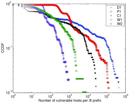
(a) Population distributions in /8 subnets.

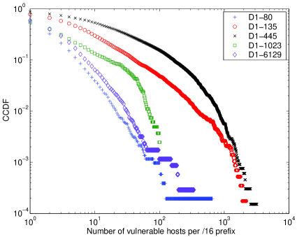
(b) Population distributions in /16 subnets.

Figure 1: CCDF of collected data sets.

IV Problem Formulation

Motivated by the empirical study, we provide a problem formulation in this section.

IV-A Characterization

Let a vulnerable host be a host that can be infected by a malware. A vulnerable host can be either already infected or uninfected. In this work, we denote vulnerable hosts as uninfected vulnerable hosts.

We consider aggregated vulnerable-host distributions. Let $l$ ($0\leq l\leq 32$) be an aggregation level of IP addresses as defined in Section III-B. For a given $l$, let $N_{i}^{(l)}$ be the number of vulnerable hosts in /$l$ subnet $i$, where $1\leq i\leq 2^{l}$. Let $N$ be the total number of vulnerable hosts, where $N=\sum_{i=1}^{2^{l}}{N_{i}^{(l)}}$. Let $p_{g}^{(l)}(i)$ ($i=1,2,\cdots,2^{l}$) be the probability that a randomly chosen vulnerable host is in the $i$-th $/l$ subnet. Then $p_{g}^{(l)}(i)=\frac{N_{i}^{(l)}}{N}$; and $\sum_{i=1}^{2^{l}}{p_{g}^{(l)}(i)}=1$. Thus, $p_{g}^{(l)}(i)$’s denote the group distribution of vulnerable hosts in /$l$ subnets.

Now consider a malware or an adversary that searches for vulnerable hosts. An adversary often does not have the complete knowledge on the locations of vulnerable hosts. Hence malwares make a random guess on which $/l$ subnets are likely to have most vulnerable hosts. This results in a class of randomized epidemic algorithms for malwares to scan subnets. Let $q_{g}^{(l)}(i)$ ($i=1,2,\cdots,2^{l}$) be the probability that a malware scans the $i$-th $/l$ subnet. As we shall see, $q_{g}^{(l)}(i)$’s characterize how effectively a malware scans and thus hits vulnerable hosts.

IV-B Examples

Consider $/8$ subnets ($l=8$). As an extreme case if all vulnerable hosts are in subnet $123.0.0.0/8$, $p_{g}^{(8)}(123)=1$ and $p_{g}^{(8)}(i)=0$ for $i\neq 123$. Hence, in view of a network defender, the network would be extremely vulnerable since if the malware discovers this subnet, the malware could focus its scan accordingly and potentially find all vulnerable hosts. As another extreme case, if $p_{g}^{(8)}(i)={1\over 2^{8}}$ is uniform, in view of a network defender, it would be harder for the malware to find vulnerable hosts rapidly as they are uniformly distributed over all /8 subnets.

In view of an adversary, whether and how vulnerable hosts can be discovered and scanned depends on a randomized algorithm utilized by the malware. In other words, an adversary can customize $q_{g}^{(l)}(i)$’s to make the malware spread either faster or slower. Specifically, for the first extreme case where all vulnerable subnets are concentrated in subnet $123.0.0.0/8$, $q_{g}^{(8)}(i)=p_{g}^{(8)}(i)$ would be the best choice, and the resulting malware would spread the fastest. But if the adversary makes a poor choice of $q_{g}^{(l)}(i)$’s being uniform across /8 subnets, the resulting malware spread would be slow. Hence $p_{g}^{(l)}(i)$’s and $q_{g}^{(l)}(i)$’s characterize the severity of network vulnerabilities and the virulence of randomized epidemic scanning algorithms, respectively.

IV-C Problems

We now consider network-aware malware attacks in view of information theory. If a malware obtains the partial information on vulnerable hosts (e.g., $p_{g}^{(l)}(i)$’s), it can extract the information (bits) to design randomize epidemic algorithms (e.g., $q_{g}^{(l)}(i)$’s). A fundamental question is how we can relate the information on vulnerable-host distributions with the performance of randomized epidemic algorithms. Specifically, we intend to study the following questions:

• What information-theoretical measure can be used to quantify the unevenness of vulnerable-host distributions?

• How much information (bits) on vulnerable hosts can be extracted by randomized epidemic algorithms utilized by malwares?

• How good are practical randomized epidemic algorithms?

• What is the effectiveness of defense methods on network-aware malwares?

V Non-Uniformity Factor

In this section, we derive a simple metric, called the non-uniformity factor, to quantify the vulnerability, i.e., the non-uniformity of a vulnerable-host distribution. We show that the non-uniformity factor is a function of Renyi entropies. We then compare the non-uniformity factor with the well-known Shannon entropy.

V-A Definition and Property

Definition: The non-uniformity factor in /$l$ subnets is defined as

$$\beta^{(l)}=2^{l}\sum_{i=1}^{2^{l}}{\left(p_{g}^{(l)}(i)\right)^{2}}.$$ (7)

One property of $\beta^{(l)}$ is that

$$\beta^{(l)}\geq\left(\sum_{i=1}^{2^{l}}{p_{g}^{(l)}(i)}\right)^{2}=1.$$ (8)

The above inequality is derived by the Cauchy-Schwarz inequality. The equality holds if and only if $p_{g}^{(l)}(i)=2^{-l}$, for $i=1,2,\cdots,2^{l}$. In other words, when the vulnerable-host distribution is uniform, $\beta^{(l)}$ achieves the minimum value 1. On the other hand, since $p_{g}^{(l)}(i)\geq 0$,

$$\beta^{(l)}\leq 2^{l}\cdot\left(\sum_{i=1}^{2^{l}}{p_{g}^{(l)}(i)}\right)^{2}=2^{l}.$$ (9)

The equality holds when $p_{g}^{(l)}(j)=1$ for some $j$ and $p_{g}^{(l)}(i)=0$, $i\not=j$, i.e., all vulnerable hosts concentrate on one subnet. This means that when the vulnerable-host distribution is extremely non-uniform, $\beta^{(l)}$ obtains the maximum value $2^{l}$. Moreover, assuming that vulnerable hosts are uniformly distributed in the first $n$ ($1\leq n\leq 2^{l}$) /$l$ subnets, i.e., $p_{g}^{(l)}(i)=\frac{1}{n}$, $i=1,2,\cdots,n$; and $p_{g}^{(l)}(i)=0$, $i=n+1,\cdots,2^{l}$, we have $\beta^{(l)}=\frac{2^{l}}{n}$. Therefore, $\beta^{(l)}$ characterizes the non-uniformity of a vulnerable-host distribution. A larger non-uniformity factor reflects a more non-uniform distribution of vulnerable hosts.

The non-uniformity factor is indeed related to a distance between a vulnerable-host distribution and a uniform distribution. Consider $L_{2}$ distance between $p_{g}^{(l)}(i)$ and the uniform distribution $p_{u}^{(l)}(i)={1\over{2^{l}}}$ for $i=1,2,\cdots,2^{l}$, where

$${||p_{g}^{(l)}-p_{u}^{(l)}||_{2}}^{2}=\sum_{i=1}^{2^{l}}{\left(p_{g}^{(l)}(i)-\frac{1}{2^{l}}\right)^{2}},$$ (10)

which leads to

$$\beta^{(l)}=2^{l}\cdot{||p_{g}^{(l)}-p_{u}^{(l)}||_{2}}^{2}+1.$$ (11)

For a given $l$, $2^{l}$ is a constant that is the size of the sample space of /$l$ subnets. Hence $\beta^{(l)}$ essentially measures the deviation of a vulnerable-host group distribution from a uniform distribution for /$l$ subnets.

How does $\beta^{(l)}$ vary with $l$? When $l=0$, $\beta^{(0)}=1$. In the other extreme where $l=32$,

$$p_{g}^{(32)}(i)=\left\{\begin{array}[]{ll}\frac{1}{N},&\mbox{address $i$ is vulnerable to the malware};\\ 0,&\mbox{otherwise},\end{array}\right.$$ (12)

which results in $\beta^{(32)}=\frac{2^{32}}{N}$. More importantly, the ratio of $\beta^{(l)}$ to $\beta^{(l-1)}$ lies between 1 and 2, as shown below.

Theorem 2

$$\beta^{(l-1)}\leq\beta^{(l)}\leq 2\beta^{(l-1)},$$ (13)

where $l\in\{1,\cdots,32\}$.

The proof of Theorem 2 is given in Appendix 1. An intuitive explanation of this theorem is as follows. For /$l$ and /$(l-1)$ subnets, group $i$ ($i=1,2,\cdots,2^{l-1}$) of /$(l-1)$ subnets is partitioned into groups $2i-1$ and $2i$ of /$l$ subnets. If vulnerable hosts in each group of /$(l-1)$ subnets are equally divided into the groups of /$l$ subnets (i.e., $p_{g}^{(l)}(2i-1)=p_{g}^{(l)}(2i)=\frac{1}{2}p_{g}^{(l-1)}(i)$, $\forall i$), then $\beta^{(l)}=\beta^{(l-1)}$. If the division of vulnerable hosts is extremely uneven for all groups (i.e., $p_{g}^{(l)}(2i-1)=0$ or $p_{g}^{(l)}(2i)=0$, $\forall i$), then $\beta^{(l)}=2\beta^{(l-1)}$. Excluding these two extreme cases, $\beta^{(l-1)}<\beta^{(l)}<2\beta^{(l-1)}$. Therefore, $\beta^{(l)}$ is a non-decreasing function of $l$. Moreover, the ratio of $\beta^{(l)}$ to $\beta^{(l-1)}$ reflects how unevenly vulnerable hosts in each /$(l-1)$ subnet distribute between two groups of /$l$ subnets. This ratio is indicated by the slope of $\beta^{(l)}$ in a $\beta^{(l)}\sim l$ figure.

V-B Estimated Non-Uniformity Factor

Figure 2 shows the non-uniformity factors estimated from our data sets. The non-uniformity factors increase with the prefix length for all data sets. Note that the y-axis is in a log scale. Thus, $\beta^{(l)}$ increases almost exponentially with a wide range of $l$. To gain intuition on how large $\beta^{(l)}$ can be, $\beta^{(8)}$ and $\beta^{(16)}$ are summarized for all data sets in Table II. It can be observed that $\beta^{(8)}$ and $\beta^{(16)}$ have large values, indicating the significant unevenness of collected distributions.

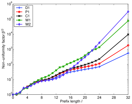
(a) Five data sets.

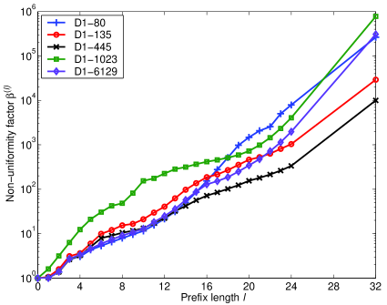
(b) D1 with different ports.

Figure 2: Non-uniformity factors of collected data sets. Note that the y-axis uses a log scale.

TABLE II: $\beta^{(8)}$ and $\beta^{(16)}$ of collected distributions.

$\beta^{(l)}$	D1	P1	C1	W1	W2
$\beta^{(8)}$	7.9	8.4	9.0	12.0	7.8
$\beta^{(16)}$	31.2	43.2	52.2	126.7	50.2
$\beta^{(l)}$	D1-80	D1-135	D1-445	D1-1023	D1-6129
$\beta^{(8)}$	7.9	15.4	10.5	48.2	9.1
$\beta^{(16)}$	153.3	186.6	71.7	416.3	128.9

V-C Shannon Entropy

To further understand the importance of the non-uniformity factor, we now turn our attention on the Shannon entropy for comparison. It is well-known that the Shannon entropy can be used to measure the non-uniformity of a probability distribution [11]. The Shannon entropy in /$l$ subnets is defined as

$$H\left(P^{(l)}\right)=-\sum_{i=1}^{2^{l}}{p_{g}^{(l)}(i)\log_{2}p_{g}^{(l)}(i)},$$ (14)

where $P^{(l)}=\{p_{g}^{(l)}(1),p_{g}^{(l)}(2),\cdots,p_{g}^{(l)}(2^{l})\}$.

It is noted that

$$0\leq H\left(P^{(l)}\right)\leq l.$$ (15)

If a distribution is uniform, $H\left(P^{(l)}\right)$ achieves the maximum value $l$. On the other hand, if a distribution is extremely non-uniform, e.g., all vulnerable hosts concentrate on one subnet, $H\left(P^{(l)}\right)$ obtains the minimum value 0.

Furthermore, we compare $H\left(P^{(l)}\right)$ with $H\left(P^{(l-1)}\right)$ and find that their difference is between 0 and 1, as shown in the following theorem.

Theorem 3

$$H\left(P^{(l-1)}\right)\leq H\left(P^{(l)}\right)\leq H\left(P^{(l-1)}\right)+1,$$ (16)

where $l\in\{1,\cdots,32\}$.

The proof of Theorem 3 is given in Appendix 2. If vulnerable hosts in each group of /$(l-1)$ subnets are extremely unevenly divided into the groups of /$l$ subnets (i.e., $p_{g}^{(l)}(2i-1)=0$ or $p_{g}^{(l)}(2i)=0$, $\forall i\in\{1,2,\cdots,2^{l-1}\}$), then $H\left(P^{(l)}\right)=H\left(P^{(l-1)}\right)$. If the division of vulnerable hosts is equal for all groups (i.e., $p_{g}^{(l)}(2i-1)=p_{g}^{(l)}(2i)=\frac{1}{2}p_{g}^{(l-1)}(i)$, $\forall i$)), then $H\left(P^{(l)}\right)=H\left(P^{(l-1)}\right)+1$. Excluding these two extreme cases, $H\left(P^{(l-1)}\right)<H\left(P^{(l)}\right)<H\left(P^{(l-1)}\right)+1$. Therefore, $H\left(P^{(l)}\right)$ is a non-decreasing function of $l$. Moreover, the difference between $H\left(P^{(l)}\right)$ and $H\left(P^{(l-1)}\right)$ reflects how evenly vulnerable hosts in each /($l-1$) subnet distribute between two groups of /$l$ subnets.

Figure 3 shows the Shannon entropies of our empirical distributions from the data sets. $H\left(P^{(l)}\right)=l$ is denoted by the diagonal line in the figure. It can be seen that the curves for our collected data sets are similar.

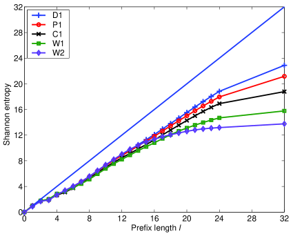
(a) Five data sets.

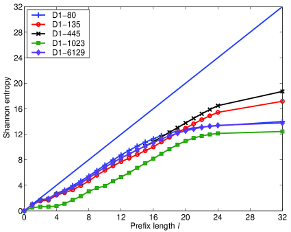
(b) D1 with different ports.

Figure 3: Shannon entropies of collected data sets.

V-D Non-Uniformity Factor, Renyi Entropy, and Shannon Entropy

To quantify the difference between the non-uniformity factor and the Shannon entropy, we note that the non-uniformity factor directly relates to the Renyi entropies of order two and zero, as shown in the following equation:

$$\beta^{(l)}=2^{l-H_{2}\left(P^{(l)}\right)}=2^{H_{0}\left(P^{(l)}\right)-H_{2}\left(P^{(l)}\right)},$$ (17)

where $P^{(l)}=\{p_{g}^{(l)}(1),p_{g}^{(l)}(2),\cdots,p_{g}^{(l)}(2^{l})\}$. Therefore, the non-uniformity factor is essentially a Renyi entropy. Hence, the non-uniformity factor corresponds to a generalized entropy of order 2, whereas the Shannon entropy is the generalized entropy of order 1.

Why do we choose the non-uniformity factor rather than the Shannon entropy? We compare these two metrics in terms of characterizing a vulnerable-host distribution and find the following fundamental differences.

• In Figure 2, when a distribution is uniform, $\beta^{(l)}=1$. Hence, the distance between $\beta^{(l)}$ and the horizontal access $1$ measures the degree of unevenness. Similarly, the distance between $H\left(P^{(l)}\right)$ and 0 in Figure 3 reflects how uniform a distribution is. A larger $H\left(P^{(l)}\right)$ corresponds to a more even distribution, whereas a larger $\beta^{(l)}$ corresponds to a more non-uniform distribution. In addition, if two distributions have different prefix lengths, we can directly apply the non-uniformity factor (or the Shannon entropy) to compare the unevenness (or evenness) between them. Therefore, the Shanon entropy provides a better measure for describing the evenness of a distribution, while the non-uniformity factor gives a better metric for characterizing the non-uniformity of a distribution.

• From Theorem 1 and Equation (17), we have $\beta^{(l)}>2^{l-H\left(P^{(l)}\right)}$ when the non-zero $p_{g}^{(l)}$’s are not all equal. Meanwhile, evidenced by Figures 2 and 3, the non-uniformity factor magnifies the unevenness of a distribution. Therefore, $\beta^{(l)}$ depends more on the large $p_{g}^{(l)}$’s.

A more important aspect of using the non-uniformity factor is its relation to some real randomized epidemic algorithms (e.g., localized scanning and sequential scanning). Such a relation cannot be drawn using the Shannon entropy. We will show this in the next section.

VI Network-Aware Malware Spreading Ability

In this section, we explicitly relate the speed of malware propagation with the information bits extracted by random-scanning and network-aware malwares.

VI-A Collision Probability, Uncertainty, and Information Bits

We begin with defining three important quantities: the collision probability, uncertainty, and information bits. Consider a randomly chosen vulnerable host $Y$. The probability that this host is in the $/l$ subnet $i$ is $p_{g}^{(l)}(i)$. Imagine that a malware guesses which subnet host $Y$ belongs to and chooses a target $/l$ subnet $i$ with the probability $q_{g}^{(l)}(i)=p_{g}^{(l)}(i)$. Thus, the probability for the malware to make a correct guess is $p_{h}=\sum_{i=1}^{2^{l}}{\left(p_{g}^{(l)}(i)\right)^{2}}$. This probability is called the collision probability and is defined in [5]. Such a probability of success is reflected in our designed non-uniformity factor and corresponds to a scenario that the malware knows the underlying vulnerable-host group distribution. Intuitively, the more non-uniform a vulnerable-host distribution is, the larger the probability of success is, i.e., the easier it is for a scan to hit a vulnerable host, the more vulnerable the network is, and the less uncertainty there is in a vulnerable-host distribution.

We now extend the concept of the collision probability and define $p_{h}$ as the probability that a malware scan hits a subnet where a randomly chosen vulnerable host locates, i.e.,

$$p_{h}=\sum_{i=1}^{2^{l}}{p_{g}^{(l)}(i)q_{g}^{(l)}(i)}.$$ (18)

Then two important quantities can be defined:

• $-\log_{2}{p_{h}}$ as the uncertainty exhibited by the vulnerable-host distribution $p_{g}^{(l)}(i)$’s.

• $H_{0}\left(P^{(l)}\right)-[-\log_{2}{p_{h}}]$ as the number of information bits extracted by a randomized epidemic scanning algorithm using $q_{g}^{(l)}(i)$’s.

Here $-\log_{2}{p_{h}}$ is regarded as the uncertainty on the vulnerable-host distribution in view of the malware, similar to self-information [39]. For example, if a malware has no information about a vulnerable-host distribution and has to use random scanning, it has the largest uncertainty $H_{0}\left(P^{(l)}\right)=l$ and extracts zero information bit from the distribution. Likewise, the number of information bits extracted by a network-aware malware can be measured as the reduction of the uncertainty and thus equals to $H_{0}\left(P^{(l)}\right)-[-\log_{2}{p_{h}}]$. For example, $\log_{2}{\beta^{(l)}}=H_{0}\left(P^{(l)}\right)-H_{2}\left(P^{(l)}\right)$ is the information bits extractable by an adversary that chooses $q_{g}^{(l)}(i)=p_{g}^{(l)}(i)$.

VI-B Infection Rate

We characterize the spread of a network-aware malware at an early stage by deriving the infection rate. The infection rate, denoted by $\alpha$, is defined as the average number of vulnerable hosts that can be infected per unit time by one infected host during the early stage of malware propagation [32]. The infection rate is an important metric for studying network-aware malware spreading ability for two reasons. First, since the number of infected hosts increases exponentially with the rate $1+\alpha$ during the early stage, a malware with a higher infection rate can spread much faster at the beginning and thus infect a large number of hosts in a shorter time [8]. Second, while it is generally difficult to derive a close-form solution for dynamic malware propagation, we can obtain a close-form expression of the infection rate for different malware scanning methods.

Let $R$ denote the (random) number of vulnerable hosts that can be infected per unit time by one infected host during the early stage of malware propagation. The infection rate is the expected value of $R$, i.e., $\alpha=E[R]$. Let $s$ be the scanning rate or the number of scans sent by an infected host per unit time, $N$ be the number of vulnerable hosts, and $\Omega$ be the scanning space (i.e., $\Omega=2^{32}$).

VI-C Random Scanning

Random scanning (RS) has been used by most real worms. For RS, an infected host sends out $s$ random scans per unit time, and the probability that one scan hits a vulnerable host is $\frac{N}{\Omega}$. Thus, $R$ follows a Binomial distribution B($s$, $\frac{N}{\Omega}$), resulting in

$$\alpha_{RS}=E[R]=\frac{sN}{\Omega}.$$ (19)

Another way to derive the infection rate of RS is as follows. Consider a randomly chosen vulnerable host $Y$. The probability that this host is in the /$l$ subnet $i$ is $p_{g}^{(l)}(i)$. An RS malware can make a successful guess on which subnet host $Y$ belongs to with collision probability $p_{h}=\frac{1}{2^{l}}=2^{-H_{0}\left(P^{(l)}\right)}$. A scan from the RS malware can be regarded as first selecting the /$l$ subnet randomly and then choosing the host in the subnet at random. Hence the probability for the malware to hit host $Y$ is $\frac{1}{2^{32-l}}\cdot 2^{-H_{0}\left(P^{(l)}\right)}=2^{-H_{0}\left(P^{(l)}\right)-(32-l)}$. Since there are $N$ vulnerable hosts, the probability for a malware to hit a vulnerable host is $N\cdot 2^{-H_{0}\left(P^{(l)}\right)-(32-l)}$. Thus, $R$ follows a Binomial distribution B($s$, $N\cdot 2^{-H_{0}\left(P^{(l)}\right)-(32-l)}$), resulting in

$$\alpha_{RS}=E[R]=\frac{sN}{2^{32-l}}\cdot 2^{-H_{0}\left(P^{(l)}\right)}.$$ (20)

Therefore, for the RS malware, the uncertainty on the vulnerable-host distribution is $-\log_{2}{p_{h}}=H_{0}\left(P^{(l)}\right)$, i.e., the number of information bits on vulnerable hosts extracted by RS is $H_{0}\left(P^{(l)}\right)-H_{0}\left(P^{(l)}\right)=0$.

VI-D Optimal Importance Scanning

Importance scanning (IS) exploits the non-uniform distribution of vulnerable hosts. We derive the infection rate of IS. An infected host scans /$l$ subnet $i$ with the probability $q_{g}^{(l)}(i)$. Consider a randomly chosen vulnerable host $Y$. The probability for this host being in /$l$ subnet $i$ is $p_{g}^{(l)}(i)$. An IS malware can make a successful guess on which subnet host $Y$ belongs to with collision probability $p_{h}=\sum_{i=1}^{2^{l}}{p_{g}^{(l)}(i)q_{g}^{(l)}(i)}$. Thus, the probability for the malware to hit the host $Y$ is $\frac{1}{2^{32-l}}\sum_{i=1}^{2^{l}}{p_{g}^{(l)}(i)q_{g}^{(l)}(i)}$. Similar to RS, $R$ of IS follows a Binomial distribution B($s$,$\frac{N}{2^{32-l}}\sum_{i=1}^{2^{l}}{p_{g}^{(l)}(i)q_{g}^{(l)}(i)}$), which leads to

$$\alpha_{IS}=E[R]=\frac{sN}{2^{32-l}}\sum_{i=1}^{2^{l}}{p_{g}^{(l)}(i)q_{g}^{(l)}(i)}.$$ (21)

Therefore, the uncertainty of the vulnerable-host distribution for an IS malware is $-\log_{2}{\sum_{i=1}^{2^{l}}{p_{g}^{(l)}(i)q_{g}^{(l)}(i)}}$, and the number of information bits on vulnerable hosts extracted by IS is $H_{0}\left(P^{(l)}\right)+\log_{2}{\sum_{i=1}^{2^{l}}{p_{g}^{(l)}(i)q_{g}^{(l)}(i)}}$.

Note that importance scanning can choose $q_{g}^{(l)}(i)$’s to maximize the infection rate, resulting in a “worst-case” scenario for defenders or /$l$ optimal IS (/$l$ OPT_IS) for attackers [8], i.e.,

$$\alpha_{OPT\_IS}^{(l)}=\max\{\alpha_{IS}\}=\frac{sN}{2^{32-l}}\max_{i}\{p_{g}^{(l)}(i)\}.$$ (22)

That is,

$$\alpha_{OPT\_IS}^{(l)}=\frac{sN}{2^{32-l}}2^{-H_{\infty}\left(P^{(l)}\right)}=\alpha_{RS}\cdot 2^{H_{0}\left(P^{(l)}\right)-H_{\infty}\left(P^{(l)}\right)}.$$ (23)

Therefore, the uncertainty on the vulnerable-host distribution for /$l$ OPT_IS is $H_{\infty}\left(P^{(l)}\right)$; and the number of infection bits on vulnerable hosts extracted by this scanning method is $H_{0}\left(P^{(l)}\right)-H_{\infty}\left(P^{(l)}\right)$.

VI-E Suboptimal Importance Scanning

As shown in our prior work [8], the optimal IS is difficult to implement in reality. Hence we also consider a special case of IS, where the group scanning distribution $q_{g}^{(l)}(i)$ is chosen to be proportional to the number of vulnerable hosts in group $i$, i.e., $q_{g}^{(l)}(i)=p_{g}^{(l)}(i)$. This results in suboptimal IS [8], called /$l$ IS. Thus, the infection rate is

$$\alpha_{IS}^{(l)}=\frac{sN}{2^{32-l}}{\sum_{i=1}^{2^{l}}\left(p_{g}(i)\right)^{2}}=\frac{sN}{2^{32-l}}{\cdot 2^{-H_{2}\left(P^{(l)}\right)}}=\alpha_{RS}\cdot\beta^{(l)}.$$ (24)

Therefore, the uncertainty on the vulnerable-host distribution for /$l$ IS is $H_{2}\left(P^{(l)}\right)$; and the corresponding number of information bits extracted is $H_{0}\left(P^{(l)}\right)-H_{2}\left(P^{(l)}\right)$ or $\log_{2}{\beta^{(l)}}$. Moreover, compared with RS, this /$l$ IS can increase the infection rate by a factor of $\beta^{(l)}$. On the other hand, RS can be regarded as a special case of suboptimal IS when $l=0$.

VI-F Localized Scanning

Localized scanning (LS) has been used by such real worms as Code Red II and Nimda. LS is a simpler randomized algorithm that utilizes only a few parameters rather than an underlying vulnerable-host group distribution. We first consider a simplified version of LS, called /$l$ LS, which scans the Internet as follows:

• $p_{a}$ ($0\leq p_{a}\leq 1$) of the time, an address with the same first $l$ bits is chosen as the target,

• $1-p_{a}$ of the time, an address is chosen randomly from an entire IP address space.

Hence LS is an oblivious yet local randomized algorithm where the locality is characterized by parameter $p_{a}$. Assume that an initially infected host is randomly chosen from the vulnerable hosts. Let $I_{g}$ denote the subnet where an initially infected host locates. Thus, $P(I_{g}=i)=p_{g}^{(l)}(i)$, where $i=1,2,\cdots,2^{l}$. For an infected host located in /$l$ subnet $i$, a scan from this host probes globally with the probability of $1-p_{a}$ and hits /$l$ subnet $j$ ($j\not=i$) with the likelihood of $\frac{1-p_{a}}{2^{l}}$. Thus, the group scanning distribution for this host is

$$q_{g}^{(l)}(j)=\left\{\begin{array}[]{ll}p_{a}+\frac{1-p_{a}}{2^{l}},&\mbox{if $j=i$};\\ \frac{1-p_{a}}{2^{l}},&\mbox{otherwise},\end{array}\right.$$ (25)

where $j=1,2,\cdots,2^{l}$. Given the subnet location of an initially infected host (i.e., /$l$ subnet $i$), the conditional collision probability or the probability for a malware scan to hit a randomly chosen vulnerable host can be calculated based on Equation (18), i.e.,

$$p_{h}(i)=p_{a}p_{g}^{(l)}(i)+\frac{1-p_{a}}{2^{l}}.$$ (26)

Therefore, we can compute the collision probability as

$$p_{h}=\sum_{i=1}^{2^{l}}{P(I_{g}=i)p_{h}(i)}=p_{a}\sum_{i=1}^{2^{l}}{p_{g}^{2}(i)}+\frac{1-p_{a}}{2^{l}},$$ (27)

resulting in

$$\alpha_{LS}^{(l)}=\alpha_{RS}\left(1-p_{a}+p_{a}\beta^{(l)}\right).$$ (28)

Therefore, the number of information bits extracted from the vulnerable-host distribution by /$l$ LS is $\log_{2}\{1-p_{a}+p_{a}\beta^{(l)}\}$, which is between 0 and $H_{0}\left(P^{(l)}\right)-H_{2}\left(P^{(l)}\right)$.

Moreover, since $\beta^{(l)}>1$ ($\beta^{(l)}=1$ is for a uniform distribution and is excluded here), $\alpha_{LS}^{(l)}$ increases with respect to $p_{a}$. Specifically, when $p_{a}\rightarrow 1$, $\alpha_{LS}^{(l)}\rightarrow\alpha_{RS}\beta^{(l)}=\alpha_{IS}^{(l)}$. Thus, /$l$ LS has an infection rate comparable to that of /$l$ IS. In reality, $p_{a}$ cannot be 1. This is because an LS malware begins spreading from one infected host that is specifically in a subnet; and if $p_{a}=1$, the malware can never spread out of this subnet. Therefore, we expect that the optimal value of $p_{a}$ should be large but not 1.

Next, we further consider another LS, called two-level LS (2LLS), which has been used by the Code Red II and Nimda worms [34, 35]. 2LLS scans the Internet as follows:

• $p_{b}$ ($0\leq p_{b}\leq 1$) of the time, an address with the same first byte is chosen as the target,

• $p_{c}$ ($0\leq p_{c}\leq 1-p_{b}$) of the time, an address with the same first two bytes is chosen as the target,

• $1-p_{b}-p_{c}$ of the time, a random address is chosen.

For example, for the Code Red II worm, $p_{b}=0.5$ and $p_{c}=0.375$ [34]; for the Nimda worm, $p_{b}=0.25$ and $p_{c}=0.5$ [35]. Using the similar analysis for /$l$ LS, we can derive the infection rate of 2LLS:

$$\alpha_{2LLS}=\alpha_{RS}\left(1-p_{b}-p_{c}+p_{b}\beta^{(8)}+p_{c}\beta^{(16)}\right).$$ (29)

Similarly, the number of information bits extracted from the vulnerable-host distribution by the 2LLS malware is $\log_{2}\{1-p_{b}-p_{c}+p_{b}\beta^{(8)}+p_{c}\beta^{(16)}\}$, which is between 0 and $H_{0}\left(P^{(16)}\right)-H_{2}\left(P^{(16)}\right)$.

Since $\beta^{(16)}\geq\beta^{(8)}\geq 1$ from Theorem 2, $\alpha_{2LLS}$ holds or increases when both $p_{b}$ and $p_{c}$ increase. Specially, when $p_{c}\rightarrow 1$, $\alpha_{2LLS}\rightarrow\alpha_{RS}\beta^{(16)}=\alpha_{IS}^{(16)}$. Thus, 2LLS has an infection rate comparable to that of /16 IS. Moreover, $\beta^{(16)}$ is much larger than $\beta^{(8)}$ as shown in Table II for the collected distributions. Hence, $p_{c}$ is more significant than $p_{b}$ for 2LLS.

VI-G Modified Sequential Scanning

The Blaster worm is a real malware that exploits sequential scanning in combination with localized scanning. A sequential-scanning malware studied in [33, 13] begins to scan addresses sequentially from a randomly chosen starting IP address and has a similar propagation speed as a random-scanning malware. The Blaster worm selects its starting point locally as the first address of its Class C subnet with probability 0.4 [37, 33]. To analyze the effect of sequential scanning, we do not incorporate localized scanning. Specifically, we consider our /$l$ modified sequential-scanning (MSS) malware, which scans the Internet as follows:

• Newly infected host $A$ begins with random scanning until finding a vulnerable host with address $B$.

• After infecting the target $B$, host $A$ continues to sequentially scan IP addresses $B+1$, $B+2$, $\cdots$ (or $B-1$, $B-2$, $\cdots$) in the /$l$ subnet where $B$ locates.

Such a sequential malware-scanning strategy is in a similar spirit to the nearest neighbor rule, which is widely used in pattern classification [10]. The basic idea is that if the vulnerable hosts are clustered, the neighbor of a vulnerable host is likely to be vulnerable also.

Such a /$l$ MSS malware has two stages. In the first stage (called MSS_1), the malware uses random scanning and has an infection rate of $\alpha_{RS}$, i.e., $\alpha_{MSS\_1}=\alpha_{RS}$. In the second stage (called MSS_2), the malware scans sequentially in a /$l$ subnet. The fist $l$ bits of a target address are fixed, whereas the last $32-l$ bits of the address are generated additively or subtractively and are modulated by $2^{32-l}$. Let $I_{g}$ denote the sunbet where $B$ locates. Thus, $P(I_{g}=i)=p_{g}^{(l)}(i)$, where $i=1,2,\cdots,2^{l}$. Since an MSS_2 malware scans only the subnet where $B$ locates, the conditional collision probability $p_{h}(i)=p_{g}^{(l)}(i)$, which leads to $p_{h}=\sum_{i=1}^{2^{l}}{\left(p_{g}^{(l)}(i)\right)^{2}}$. Thus, the infection rate is

$$\alpha_{MSS\_2}=\alpha_{RS}\cdot\beta^{(l)}.$$ (30)

Therefore, the uncertainty on vulnerable hosts for /$l$ MSS is between $H_{0}\left(P^{(l)}\right)$ and $H_{2}\left(P^{(l)}\right)$. Moreover, the infection rate of /$l$ MSS is between $\alpha_{RS}$ and $\alpha_{RS}\beta^{(l)}$.

VI-H Summary

In summary, the uncertainty on the vulnerable-host distribution and the corresponding number of information bits extracted by different randomized epidemic algorithms depends on the Renyi entropies of different orders, as shown in Table III. Moreover, the number of the information bits extractable by the network-aware malwares bridges the entropy on a vulnerable-host distribution and the malware propagation speed, as shown in the following equation.

$$\mbox{Information bits}=H_{0}\left(P^{(l)}\right)-[-\log_{2}{p_{h}}]=\log_{2}\left\{\frac{\alpha}{\alpha_{RS}}\right\},$$ (31)

where $p_{h}$ is the collision probability and $\alpha$ is the infection rate of the malware.

TABLE III: Summary of Randomized Epidemic Scanning Algorithms and Information Bits

Algorithm	Infection Rate	Information Bits Extracted
RS	$\frac{sN}{2^{32-l}}\cdot 2^{-H_{0}\left(P^{(l)}\right)}$	$0$
/$l$ OPT_IS	$\alpha_{RS}\cdot 2^{H_{0}\left(P^{(l)}\right)-H_{\infty}\left(P^{(l)}\right)}$	$H_{0}\left(P^{(l)}\right)-H_{\infty}\left(P^{(l)}\right)$
/$l$ IS	$\alpha_{RS}\cdot\beta^{(l)}$	$\log_{2}\{\beta^{(l)}\}$
/$l$ LS	$\alpha_{RS}\left(1-p_{a}+p_{a}\beta^{(l)}\right)$	$\log_{2}\{1-p_{a}+p_{a}\beta^{(l)}\}$
2LLS	$\alpha_{RS}\left(1-p_{b}-p_{c}+p_{b}\beta^{(8)}+p_{c}\beta^{(16)}\right)$	$\log_{2}\{1-p_{b}-p_{c}+p_{b}\beta^{(8)}+p_{c}\beta^{(16)}\}$
/$l$ MSS_2	$\alpha_{RS}\cdot\beta^{(l)}$	$\log_{2}\{\beta^{(l)}\}$

When /$l$ subnets are considered, RS has the largest uncertainty $H_{0}\left(P^{(l)}\right)$, while optimal IS has the smallest uncertainty $H_{\infty}\left(P^{(l)}\right)$. Moreover, infection rates of all three network-aware malwares (suboptimal IS, LS, and MSS) can be far larger than that of an RS malware, depending on the non-uniformity factors (i.e., $\beta^{(l)}$) or the Renyi entropy in the order of two (i.e., $H_{2}\left(P^{(l)}\right)$). The infection rates of all these scanning algorithms are characterized by the Renyi entropies, relating the efficiency of a randomized scanning algorithm with the information bits in a non-uniform vulnerable-host distribution.

Hence we relate the information theory with the network-aware malware propagation through the Renyi entropy. The uncertainty of a vulnerable-host group probability distribution, which is quantified by the Renyi entropy, is important for an attacker to design a network-aware malware. If there is no uncertainty about the distribution of vulnerable hosts (e.g., either all vulnerable hosts are concentrated on a subnet or all information about vulnerable hosts is known), the entropy is minimum, and the malware that uses the information on the distribution can spread fastest by employing the optimal importance scanning. On the other hand, if there is maximum uncertainty (e.g., vulnerable hosts are uniformly distributed), the entropy is maximum. For this case, the best a malware can take an advantage from a uniform distribution is to use random scanning. In general, when an attacker obtains more information about a non-uniform vulnerable-host distribution, the resulting malware can spread faster.

VII Simulation and Validation

We now validate our analytical results through simulations on the collected data sets.

VII-A Infection Rate

We first focus on validating infection rates. We apply the discrete event simulation to our experiments [23]. Specifically, we simulate the searching process of a malware using different scanning methods at the early stage. We use the C1 data set for the vulnerable-host distribution. Note that the C1 distribution has the non-uniformity factors $\beta^{(8)}=9.0$ and $\beta^{(16)}=52.2$, and $\max_{i}\{p_{g}^{(l)}(i)\}=0.0041$. The malware spreads over the C1 distribution with $N=448,894$ and has a scanning rate $s=100$. The uncertainty on the vulnerable-host distribution and the information bits extractable for different scanning methods are shown in Table IV. The simulation stops when the malware has sent out $10^{3}$ scans for RS, /16 OPT_IS, /16 IS, /16 LS, and 2LLS, and 65,535 scans for /16 MSS_2. Then, we count the number of vulnerable hosts hit by the malware scans and compute the infection rate. The results are averaged over $10^{4}$ runs. Table IV compares the simulation results (i.e., sample mean) with the analytical results (i.e., Equations (20), (22), (24), (28), (29), and (30)). Here, a /16 LS malware uses $p_{a}=0.75$, whereas a 2LLS malware employs $p_{b}=0.25$ and $p_{c}=0.5$. We observe that the sample means and the analytical results are almost identical.

TABLE IV: Uncertainty on the vulnerable-host distribution, information bits, and infection rates of different scanning methods.

Scanning method	RS	/16 OPT_IS	/16 IS	/16 LS	2LLS	/16 MSS_2
Uncertainty (analytical result)	16	7.9266	10.2940	10.6999	11.1620	10.2940
Information bits (analytical result)	0	8.0734	5.7060	5.3001	4.8380	5.7060
Infection rate (analytical result)	0.0105	2.8152	0.5456	0.4118	0.2989	0.5456
Infection rate (sample mean)	0.0103	2.7745	0.5454	0.4023	0.2942	0.5489
Infection rate (sample variance)	0.0010	0.2597	0.0543	0.2072	0.1053	0.3186

We observe that network-aware malwares have much larger infection rates than random-scanning malwares. LS indeed increases the infection rate with nearly a non-uniformity factor and approaches the capacity of suboptimal IS. This is significant as LS only depends on one or two parameters (i.e., $p_{a}$ for /$l$ LS and $p_{b}$, $p_{c}$ for 2LLS), while IS requires the information of the vulnerable-host distribution. On the other hand, LS has a larger sample variance than IS as indicated by Table IV. This implies that the infection speed of an LS malware depends on the location of initially infected hosts. If the LS malware begins spreading from a subnet containing densely populated vulnerable hosts, the malware would spread rapidly. Furthermore, we notice that the MSS malware also has a large infection rate at the second stage, indicating that MSS can indeed exploit the clustering pattern of the distribution. Meanwhile, the large sample variance of the infection rate of MSS_2 reflects that an MSS malware strongly depends on the initially infected hosts. We further compute the infection rate of a /16 MSS malware that includes both random-scanning and sequential-scanning stages. Simulation results are averaged over $10^{6}$ runs and are summarized in Table V. These results strongly depend on the total number of malware scans. When the number of malware scans is small, an MSS malware behaves similar to a random-scanning malware. When the number of malware scans increases, the MSS malware spends more scans on the second stage and thus has a larger infection rate.

TABLE V: Infection rates of a /16 MSS malware.

# of malware scans	10	100	1000	10000	50000
Sample mean	0.0108	0.0190	0.0728	0.2866	0.4298
Sample variance	0.1246	0.1346	0.1659	0.2498	0.2311

VII-B Dynamic Malware Propagation

An infection rate only characterizes the early stage of malware propagation. We now employ the analytical active worm propagation (AAWP) model and its extensions to characterize the entire spreading process of malwares [6]. Specifically, the spread of RS and IS malwares is implemented as described in [8], whereas the propagation of LS malwares is modeled according to [19]. The parameters that we use to simulate a malware are comparable to those of the Code Red v2 worm. Code Red v2 has a vulnerable population $N=360,000$ and a scanning rate $s=358$ per minute [31]. We assume that the malware begins spreading from an initially infected host that is located in the subnet containing the largest number of vulnerable hosts.

We first show the propagation speeds of network-aware malwares for the same vulnerable-host distribution from data set D1-80. From Section VI, we expect that a network-aware malware can spread much faster than an RS malware. Figure 4 demonstrates such an example on a malware that uses different scanning methods. It takes an RS malware 10 hours to infect 99% of vulnerable hosts, whereas a /8 LS malware with $p_{a}=0.75$ or a /8 IS malware takes only about 3.5 hours. A /16 LS malware with $p_{a}=0.75$ or a 2LLS malware with $p_{b}=0.25$ and $p_{c}=0.5$ can further reduce the time to 1 hour. A /16 IS malware spreads fastest and takes only 0.5 hour.

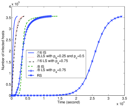
Figure 4: A network-aware malware spreads over the D1-80 distribution.

We also study the effect of vulnerable-host distributions on the propagation of network-aware malwares. From Table II, we observe that $\beta_{D1-1023}^{(16)}>\beta_{W1}^{(16)}>\beta_{C1}^{(16)}>\beta_{D1}^{(16)}$. Thus, we expect that a network-aware malware using the /16 D1-1023 distribution would spread faster than using other three distributions. Figure 5 verifies this through the simulations of the spread of a 2LLS malware that uses different vulnerable-host distributions (i.e., D1-1023, W1, C1, and D1). Here, the 2LLS malware employs the same parameters as the Nimda worm, i.e., $p_{b}=0.25$ and $p_{c}=0.5$. As expected, the malware using the D1-1023 distribution spreads fastest, especially at the early stage of malware propagation.

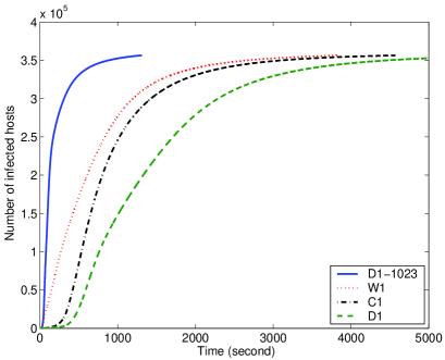
Figure 5: A 2LLS malware spreads over different distributions.

VIII Effectiveness of defense strategies

What are new requirements and challenges for a defense system to slow down the spread of a network-aware malware? We study the effectiveness of defense strategies through non-uniformity factors.

VIII-A Host-Based Defense

Host-based defense has been widely used for random-scanning malwares. Proactive protection and virus throttling are examples of host-based defense strategies.

A proactive protection (PP) strategy proactively hardens a system, making it difficult for a malware to exploit vulnerabilities [4]. Techniques used by PP include address-space randomization, pointer encryption, instruction-set randomization, and password protection. Thus, a malware requires multiple trials to compromise a host that implements PP. Specifically, let $p$ ($0\leq p\leq 1$) denote the protection probability or the probability that a single malware attempt succeeds in infecting a vulnerable host that implements PP. On the average, a malware should make $\frac{1}{p}$ exploit attempts to compromise the target. We assume that hosts with PP are uniformly deployed in the Internet. Let $d$ ($0<d\leq 1$) denote the deployment ratio of the number of hosts with PP to the total number of hosts.

To show the effectiveness of the PP strategy, we consider the infection rate of a /$l$ IS malware. Since now some of the vulnerable hosts implement PP, Equation (24) changes to

$$\alpha_{IS}^{(l)} = \frac{sN}{2^{32-l}}\sum_{i=1}^{2^{l}}{\left[dp\left(p_{g}^{(l)}(i)\right)^{2}+(1-d)\left(p_{g}^{(l)}(i)\right)^{2}\right]}$$ (32)

$$= \alpha_{RS}\beta^{(l)}(1-d+dp).$$

To slow down the spread of a suboptimal IS malware to that of a random-scanning malware, $\beta^{(l)}(1-d+dp)\leq 1$, resulting in

$$p\leq\frac{1-(1-d)\beta^{(l)}}{d\beta^{(l)}}.$$ (33)

When PP is fully deployed, i.e., $d=1$, $p$ can be at most $\frac{1}{\beta^{(l)}}$. On the other hand, if PP provides perfect protection, i.e., $p=0$, $d$ should be at least $1-\frac{1}{\beta^{(l)}}$. Therefore, when $\beta^{(l)}$ is large, Inequality (33) presents high requirements for the PP strategy. For example, if $\beta^{(16)}=50$ (most of $\beta^{(16)}$’s in Table II are larger than this value), $p\leq 0.02$ and $d\geq 0.98$. That is, a PP strategy should be almost fully deployed and provide a nearly perfect protection for a vulnerable host.

We extend the model described in [8] to characterize the spread of suboptimal IS malwares under the defense of the PP strategy and show the results in Figure 6. Here, Code-Red-v2-like malwares spread over the C1 distribution with $\beta^{(16)}=52.2$. It is observed that even when the protection probability is small (e.g., $p=0.01$) and the deployment ratio is high (e.g., $d=0.8$), a /16 IS malware is slowed down a little at the early stage, compared with a /16 IS malware without the PP defense (i.e., $p=1$ and $d=0$). Moreover, when $p$ is small (e.g., $p\leq 0.02$), $d$ is a more sensitive parameter than $p$.

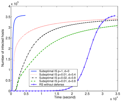
Figure 6: A /16 IS malware spreads under the defense of PP.

We next consider the virus throttling (VT) strategy [27]. VT constrains the number of outgoing connections of a host and can thus reduce the scanning rate of an infected host. We find that Equation (32) also holds for this strategy, except that $p$ is the ratio of the scanning rate of infected hosts with VT to that of infected hosts without VT. Therefore, VT also requires to be almost fully deployed for fighting network-aware malwares effectively.

From these two strategies, we have learned that an effective strategy should reduce either $\alpha_{RS}$ or $\beta^{(l)}$. Host-based defense, however, is limited in such capabilities.

VIII-B IPv6

IPv6 can decrease $\alpha_{RS}$ significantly by increasing the scanning space [32]. But the non-uniformity factor would increase the infection rate if the vulnerable-host distribution is still non-uniform. Hence, an important question is whether IPv6 can counteract network-aware malwares when both $\alpha_{RS}$ and $\beta^{(l)}$ are taken into consideration.

We study this issue by computing the infection rate of a network-aware malware in the IPv6 Internet. As pointed out by [3], a smart malware can first detect some vulnerable hosts in /64 subnets containing many vulnerable hosts, then release to the hosts on the hitlist, and finally spread inside these subnets. Such a malware only scans the local /64 subnet. Thus, we focus on the spreading speed of a network-aware malware in a /64 subnet. From Figure 2, we extrapolate that $\beta^{(32)}$ in the IPv6 Internet can be in the order of $10^{5}$ if hosts are still distributed in a clustered fashion. Using the parameters $N=10^{8}$ proposed by [12] and $s=4,000$ used by the Slammer worm [17], we derive the infection rate of a /32 IS malware in a /64 subnet of the IPv6 Internet: $\alpha_{IS}^{IPv6}=\frac{sN}{2^{64}}\cdot\beta^{(32)}=2.2\times 10^{-3}$. $\alpha_{IS}^{IPv6}$ is larger than the infection rate of the Code Red v2 worm in the IPv4 Internet, where $\alpha_{RS}^{CR}=\frac{360,000\times 358/60}{2^{32}}=5\times 10^{-4}$.

Therefore, IPv6 can only slow down the spread of a network-aware malware to that of a random-scanning malware in IPv4. To defend against the malware effectively, we should further consider how to slow down the increase rate of $\beta^{(l)}$ as $l$ increases when IPv4 is updated to IPv6. In essence, we should reduce the information bits extractable by the network-aware malwares from the vulnerable-host distribution.

IX Conclusions

In this paper, we have first obtained and characterized empirical vulnerable-host distributions, using five large measurement sets from different sources. We have derived a simple metric, known as the non-uniformity factor, to quantify an uneven distribution of vulnerable hosts. The non-uniformity factors have been obtained on the empirical vulnerable-host distributions using our collected data, and all of which demonstrate large values. This implies that the non-uniformity of the vulnerable-host distribution is significant and seems to be consistent across networks and applications. Moreover, the non-uniformity factor, shown as a function of the Renyi entropies of order two and zero, better characterizes the uneven feature of a distribution than the Shannon entropy.

We have drawn a relationship between Renyi entropies and randomized epidemic scanning algorithms. In particular, we have quantified the spreading ability of network-aware malwares that utilize randomized scanning algorithms at the early stage. These randomized malware-scanning algorithms range from optimal randomized scanning (e.g., importance scanning) to real malware scanning (e.g., localized scanning). We have derived analytical expressions relating the infection rates of network-aware malwares with the uncertainty (i.e., Renyi entropy) of finding vulnerable hosts. We have derived and empirically verified that localized scanning and modified sequential scanning can increase the infection rate by nearly a non-uniformity factor when compared to random scanning and thus approach the capacity of suboptimal importance scanning. As a result, we have bridged the information bits extracted by malwares from a vulnerable-host distribution with the propagation speed of network-aware malwares.

Furthermore, we have evaluated the effectiveness of several commonly used defense strategies on network-aware malwares. The host-based defense, such as proactive protection or virus throttling, requires to be almost fully deployed to slow down malware spreading at the early stage. This implies that host-based defense would be weakened significantly by network-aware scanning. More surprisingly, different from previous findings, we have shown that network-aware malwares can be zero-day malwares in the IPv6 Internet if vulnerable hosts are still clustered. These findings present a significant challenge to malware defense: Entirely different strategies may be needed for fighting against network-aware malwares.

The information-theoretical view of malware attacks provides us a quantification and a better understanding of three aspects: a non-uniform vulnerable-host distribution characterized by the non-uniformity factor or the Renyi entropy of order two, randomized malware-scanning algorithms characterized by the infection rate or the Renyi entropy of different orders, and the effectiveness of defense strategies.

As part of our ongoing work, we plan to study in more depth relationships between information theory and dynamic malware attacks for developing effective detection and defense systems that would take vulnerable-host distributions into consideration.

APPENDIX

APPENDIX 1: Proof of Theorem 2

Proof: Group $i$ ($i=1,2,\cdots,2^{l-1}$) of /$(l-1)$ subnets is partitioned into groups $2i-1$ and $2i$ of /$l$ subnets. Thus,

$$p_{g}^{(l-1)}(i)=p_{g}^{(l)}(2i-1)+p_{g}^{(l)}(2i),$$ (A-1)

where $i=1,2,\cdots,2^{i-1}$. Then, $\beta^{(l)}$ is related to $\beta^{(l-1)}$ by the Cauchy-Schwarz inequality.

$$\beta^{(l)} = 2^{l-1}\sum_{i=1}^{2^{l-1}}\left\{\left(\sum_{j=1}^{2}{1^{2}}\right)\left[\sum_{j=1}^{2}\left(p_{g}^{(l)}(2(i-1)+j)\right)^{2}\right]\right\}$$ (A-2)

$$\geq 2^{l-1}\sum_{i=1}^{2^{l-1}}{\left(\sum_{j=1}^{2}{p_{g}^{(l)}(2(i-1)+j)}\right)^{2}}$$

$$= \beta^{(l-1)}.$$

The equality holds when $p_{g}^{(l)}(2i-1)=p_{g}^{(l)}(2i)=\frac{p_{g}^{(l-1)}(i)}{2}$, $i=1,2,\cdots,2^{l-1}$. That is, in each /$(l-1)$ subnet, the vulnerable hosts are uniformly distributed in two groups of /$l$ subnets.

On the other hand, since

$$\left(p_{g}^{(l)}(2i-1)\right)^{2}+\left(p_{g}^{(l)}(2i)\right)^{2}\leq\left(p_{g}^{(l)}(2i-1)+p_{g}^{(l)}(2i)\right)^{2},$$ (A-3)

we have

$$\frac{\beta^{(l)}}{\beta^{(l-1)}} = 2\cdot\frac{\sum_{i=1}^{2^{l-1}}\left[\left(p_{g}^{(l)}(2i-1)\right)^{2}+\left(p_{g}^{(l)}(2i)\right)^{2}\right]}{\sum_{i=1}^{2^{l-1}}{\left(p_{g}^{(l-1)}(i)\right)^{2}}}$$ (A-4)

$$\leq 2.$$

The equality holds when for $\forall i$, $p_{g}^{(l)}(2i-1)=0$ or $p_{g}^{(l)}(2i)=0$. That is, in each /$(l-1)$ subnet, the vulnerable hosts are extremely non-uniformly distributed in two groups of /$l$ subnets.  

APPENDIX 2: Proof of Theorem 3

Proof: Since

$$p_{g}^{(l-1)}(i)=\sum_{j=1}^{2}{p_{g}^{(l)}(2(i-1)+j)}\geq p_{g}^{(l)}(2(i-1)+j),$$ (A-5)

where $i=1,2,\cdots,2^{l-1}$, we have

$$H\left(P^{(l)}\right)$$

$$=-\sum_{i=1}^{2^{l-1}}{\sum_{j=1}^{2}{p_{g}^{(l)}(2(i-1)+j)\log_{2}p_{g}^{(l)}(2(i-1)+j)}}$$

$$\geq-\sum_{i=1}^{2^{l-1}}{\sum_{j=1}^{2}{p_{g}^{(l)}(2(i-1)+j)\log_{2}p_{g}^{(l-1)}(i)}}$$

$$=H\left(P^{(l-1)}\right).$$ (A-6)

The equality holds when for $\forall i$, $p_{g}^{(l)}(2i-1)=0$ or $p_{g}^{(l)}(2i)=0$. That is, in each /$(l-1)$ subnet, the vulnerable hosts are extremely non-uniformly distributed in two groups of /$l$ subnets.

On the other hand, using the log-sum inequality,

$$\sum_{j=1}^{2}{p_{g}^{(l)}(2(i-1)+j)\log_{2}{p_{g}^{(l)}(2(i-1)+j)}}$$

$$\geq\left(\sum_{j=1}^{2}{p_{g}^{(l)}(2(i-1)+j)}\right)\log_{2}{\frac{\sum_{j=1}^{2}{p_{g}^{(l)}(2(i-1)+j)}}{2}},$$ (A-7)

we have

$$H\left(P^{(l)}\right)$$

$$=-\sum_{i=1}^{2^{l-1}}{\sum_{j=1}^{2}{p_{g}^{(l)}(2(i-1)+j)\log_{2}p_{g}^{(l)}(2(i-1)+j)}}$$

$$\leq-\sum_{i=1}^{2^{l-1}}{\left(p_{g}^{(l-1)}(i)\right)\log_{2}{\frac{p_{g}^{(l-1)}(i)}{2}}}$$

$$=H\left(P^{(l-1)}\right)+1.$$ (A-8)

The equality holds when for $\forall i$, $p_{g}^{(l)}(2i-1)=p_{g}^{(l)}(2i)=\frac{p_{g}^{(l-1)}(i)}{2}$. That is, in each /$(l-1)$ subnet, the vulnerable hosts are uniformly distributed in two groups of /$l$ subnets.  

Zesheng Chen is an Assistant Professor at the Department of Electrical and Computer Engineering at Florida International University. He received his M.S. and Ph.D. degrees from the School of Electrical and Computer Engineering at the Georgia Institute of Technology in 2005 and 2007, under the supervision of Dr. Chuanyi Ji. He also holds B.E. and M.E. degrees from the Department of Electronic Engineering at Shanghai Jiao Tong University, Shanghai, China in 1998 and 2001, respectively. His research interests include network security and the performance evaluation of computer networks.

Chuanyi Ji (S’85-M’91-SM’07) is an Associate Professor at the School of Electrical and Computer Engineering at the Georgia Institute of Technology. She received a BS (Honor) from Tsinghua University, Beijing, China in 1983, an MS from the University of Pennsylvania, Philadelphia in 1986, and a PhD from the California Institute of Technology, Pasadena, in 1992, all in Electrical Engineering. Chuanyi Ji was on the faculty at Rensselaer Polytechnic Institute from 1991 to 2001. She spent her sabbatical at Bell-labs Lucent in 1999, and was a visiting faculty at MIT in Fall 2000. Chuanyi Ji’s research lies in the areas of network management and control, and adaptive learning systems. Her research interests are in understanding and managing complex networks, applications of adaptive learning systems to network management, learning algorithms, statistics, and information theory. Chuanyi Ji received CAREER award from NSF in 1995 and Early Career award from Rensselaer Polytechnic Institute in 2000.

References

- [1] S. Antonatos, P. Akritidis, E. Markatos, and K. G. Anagnostakis, “Defending against hitlist worms using network address space randomization,” in Proc. ACM/CCS Workshop on Rapid Malcode (WORM’05), Fairfax, VA, Nov. 2005, pp. 30-40.
- [2] P. Barford, R. Nowak, R. Willett, and V. Yegneswaran, “Toward a model for sources of Internet background radiation,” in Proc. of the Passive and Active Measurement Conference (PAM’06), Mar. 2006.
- [3] S. M. Bellovin, B. Cheswick, and A. Keromytis, “Worm propagation strategies in an IPv6 Internet,” ;login:, vol. 31, no. 1, Feb. 2006, pp. 70-76.
- [4] D. Brumley, L. Liu, P. Poosankam, and D. Song, “Design space and analysis of worm defense strategies,” in ACM Symposium on InformAtion, Computer and Communications Security (ASIACCS), Mar. 2006.
- [5] C. Cachin, “Entropy measures and unconditional security in cryptography,” Ph.D thesis, Swiss Federal Institute of Technology, Zurich, 1997.
- [6] Z. Chen, L. Gao, and K. Kwiat, “Modeling the spread of active worms,” in Proc. of INFOCOM’03, vol. 3, San Francisco, CA, Apr. 2003, pp. 1890-1900.
- [7] Z. Chen and C. Ji, “A self-learning worm using importance scanning,” in Proc. ACM/CCS Workshop on Rapid Malcode (WORM’05), Fairfax, VA, Nov. 2005, pp. 22-29.
- [8] Z. Chen and C. Ji, “Optimal worm-scanning method using vulnerable-host distributions,” International Journal of Security and Networks: Special Issue on Computer and Network Security, vol. 2, no. 1/2, 2007.
- [9] Z. Chen and C. Ji, “Measuring network-aware worm spreading ability,” in Proc. of INFOCOM’07, Anchorage, AK, May 2007.
- [10] T. M. Cover and P. E. Hart, “Nearest neighbor pattern classification,” IEEE Transactions on Information Theory, vol. IT-13, no. 1, Jan. 1967, pp. 21-27.
- [11] T. M. Cover and J. A. Thomas, Elements of Information Theory. New York: Wiley, 1991.
- [12] H. Feng, A. Kamra, V. Misra, and A. D. Keromytis, “The effect of DNS delays on worm propagation in an IPv6 Internet,” in Proc. of INFOCOM’05, vol. 4, Miami, FL, Mar. 2005, pp. 2405-2414.
- [13] G. Gu, M. Sharif, X. Qin, D. Dagon, W. Lee, and G. Riley, “Worm detection, early warning and response based on local victim information,” in Proc. 20th Ann. Computer Security Applications Conf. (ACSAC’04), Tucson, AZ, Dec. 2004.
- [14] G. Gu, Z. Chen, P. Porras, and W. Lee, “Misleading and defeating importance-scanning malware propagation,” in Proc. of the 3rd International Conference on Security and Privacy in Communication Networks (SecureComm’07), Nice, France, Sept. 2007.
- [15] E. Kohler, J. Li, V. Paxson, and S. Shenker, “Observed structure of addresses in IP traffic,” in ACM SIGCOMM Internet Measurement Workshop, Marseille, France, Nov. 2002.
- [16] D. Moore, C. Shannon, and J. Brown, “Code-Red: a case study on the spread and victims of an Internet worm,” in ACM SIGCOMM Internet Measurement Workshop, Marseille, France, Nov. 2002.
- [17] D. Moore, V. Paxson, S. Savage, C. Shannon, S. Staniford, and N. Weaver, “Inside the Slammer worm,” IEEE Security and Privacy, vol. 1, no. 4, July 2003, pp. 33-39.
- [18] Y. Pryadkin, R. Lindell, J. Bannister, and R. Govindan, “An empirical evaluation of IP address space occupancy,” Technical Report ISI-TR-2004-598, USC/Information Sciences Institute, Nov. 2004.
- [19] M. A. Rajab, F. Monrose, and A. Terzis, “On the effectiveness of distributed worm monitoring,” in Proc. of the 14th USENIX Security Symposium (Security’05), Baltimore, MD, Aug. 2005, pp. 225-237.
- [20] M. A. Rajab, F. Monrose, and A. Terzis, “Fast and evasive attacks: highlighting the challenges ahead,” in Proc. of the 9th International Symposium on Recent Advances in Intrusion Detection (RAID’06), Hamburg, Germany, Sept. 2006.
- [21] A. Renyi, Probability Theory. North-Holland, Amsterdam, 1970.
- [22] A. Renyi, “Some fundamental questions of information theory,” Selected Papers of Alfred Renyi, Akademiai Kiado, Budapest, vol. 2, 1976, pp. 526-552.
- [23] S. M. Ross, Simulation, 3rd Edition. Academic Press, 2002.
- [24] C. Shannon and D. Moore, “The spread of the Witty worm,” IEEE Security and Privacy, vol. 2, no. 4, Jul-Aug 2004, pp. 46-50.
- [25] S. Staniford, V. Paxson, and N. Weaver, “How to 0wn the Internet in your spare time,” in Proc. of the 11th USENIX Security Symposium (Security’02), San Francisco, CA, Aug. 2002.
- [26] S. Staniford, D. Moore, V. Paxson, and N. Weaver, “The top speed of flash worms,” in Proc. ACM/CCS Workshop on Rapid Malcode (WORM’04), Washington DC, Oct. 2004, pp. 33-42.
- [27] J. Twycross and M. M. Williamson, “Implementing and testing a virus throttle,” in Proc. of the 12th USENIX Security Symposium (Security’03), Washington, DC, Aug. 2003, pp. 285-294.
- [28] M. Vojnovic, V. Gupta, T. Karagiannis, and C. Gkantsidis, “Sampling strategies for epidemic-style information dissemination,” Technical Report, MSR-TR-2007-82, 2007.
- [29] J. Wu, S. Vangala, L. Gao, and K. Kwiat, “An effective architecture and algorithm for detecting worms with various scan techniques,” in Proc. 11th Ann. Network and Distributed System Security Symposium (NDSS’04), San Diego, CA, Feb. 2004.
- [30] V. Yegneswaran, P. Barford, and D. Plonka, “On the design and utility of Internet sinks for network abuse monitoring,” in Proc. of Symposium on Recent Advances in Intrusion Detection (RAID’04), 2004.
- [31] C. C. Zou, L. Gao, W. Gong, and D. Towsley, “Monitoring and early warning for Internet worms,” in 10th ACM Conference on Computer and Communication Security (CCS’03), Washington DC, Oct. 2003.
- [32] C. C. Zou, D. Towsley, W. Gong, and S. Cai, “Routing worm: a fast, selective attack worm based on IP address information,” in Proc. 19th ACM/IEEE/SCS Workshop on Principles of Advanced and Distributed Simulation (PADS’05), Monterey, CA, June 2005.
- [33] C. C. Zou, D. Towsley, and W. Gong, “On the performance of Internet worm scanning strategies,” Elsevier Journal of Performance Evaluation, vol. 63. no. 7, July 2006, pp. 700-723.
- [34] CERT Coordination Center, “‘Code Red II:’ another worm exploiting buffer overflow in IIS indexing service DLL,” CERT Incident Note IN-2001-09, http://www.cert.org/incident_notes/IN-2001-09.html.
- [35] CERT Coordination Center, CERT Advisory CA-2001-26 Nimda Worm, http://www.cert.org/advisories/CA-2001-26.html.
- [36] Distributed Intrusion Detection System (DShield), http://www.dshield.org/.
- [37] eEye Digital Security, “ANALYSIS: Blaster worm,” http://www.eeye.com/html/Research/Advisories/AL20030811.html.
- [38] Internet Protocol V4 Address Space, http://www.iana.org/assignments/ipv4-address-space.
- [39] Wikipedia, “Self-information,” http://en.wikipedia.org/wiki/Self-information.