Breakdown of large-$N$ quenched reduction
in $SU(N)$ lattice gauge theories

Abstract

We study the validity of the large-$N$ equivalence between four-dimensional $SU(N)$ lattice gauge theory and its momentum quenched version—the Quenched Eguchi-Kawai (QEK) model. We find that the assumptions needed for the proofs of equivalence do not automatically follow from the quenching prescription. We use weak-coupling arguments to show that large-$N$ equivalence is in fact likely to break down in the QEK model, and that this is due to dynamically generated correlations between different Euclidean components of the gauge fields. We then use Monte-Carlo simulations at intermediate couplings with $20\leq N\leq 200$ to provide strong evidence for the presence of these correlations and for the consequent breakdown of reduction. This evidence includes a large discrepancy between the transition coupling of the “bulk” transition in lattice gauge theories and the coupling at which the QEK model goes through a strongly first-order transition. To accurately measure this discrepancy we adapt the recently introduced Wang-Landau algorithm to gauge theories.

I Introduction

QCD simplifies in the ‘t Hooft limit of a large number of colors, yet differs from the physical case, $N=3$, by only $O(1/N)$ corrections tHooft ; Witten . As a result, it has been a long-standing goal to understand the properties of QCD at large $N$. This goal has become even more interesting as string theory developments, based on gauge/gravity duality, attempt to move towards predictions for QCD-like theories at infinite $N$ Zamaklar-review . Considerable progress towards this goal has been made using numerical lattice computations (as reviewed, for example, in Refs. Mike-dublin-05 ; Narayanan-Regensburg-07 ). For example, using conventional large volume simulations, and extrapolating from $N=3-16$, precision results for several quantities in the large-$N$ limit have been obtained. In addition, many quantities have been found to depend only weakly on $N$.

In this paper we reconsider an alternative to conventional large volume simulations, namely the use of large-$N$ volume reduction, in which the infinite space-time volume is collapsed to a single point, with space-time degrees of freedom repackaged into the $O(N^{2})$ color degrees of freedom. This allows one, in principle, to trade two large parameters, the volume and $N^{2}$, for a single large parameter, and consequently to consider much large values of $N$.

The idea of large-$N$ reduction for lattice gauge theories was first proposed by Eguchi and Kawai in Ref. EK . They defined the “reduced” theory to be a lattice gauge theory on a single site and showed that, under certain assumptions, Wilson loops in the reduced theory and in the $d$-dimensional infinite-lattice gauge theory acquire the same expectation values in the large-$N$ limit. The two main assumptions in EK are that expectation values of products of single-trace operators factorize at large-$N$ (see Eq. (9) below) and that the vacuum is symmetric under the $(Z_{N})^{d}$ center transformations applied to the model’s $SU(N)$ “link” matrices $U_{\mu}$ (see Eq. (5)). It was quickly realized, based on weak coupling arguments and numerical results, that the second assumption does not hold for $d>2$ in the continuum BHN1 ; MK ; Okawa1 , and various ideas for solving this problem were suggested. The first, which we focus on here, was of quenching the eigenvalues of the link matrices by forcing them to have a $Z_{N}$ invariant distribution. This means that, by construction, all order parameters for the breakdown of the $(Z_{N})^{d}$ symmetry, such as $\langle{\text{t}r}\,U_{\mu}\rangle$, vanish.

This “quenched Eguchi-Kawai” (QEK) model was proposed in Ref. BHN1 (see also Migdal ), and first numerical results indicated that it did indeed solve the problem of unwanted symmetry breaking BHN2 ; Okawa2 ; Bhanot ; BM ; Lewis ; Carlson . Intensive analytic investigation of the QEK model ensued. (For example, see the papers HN ; GK ; DW ; Parisi-papers ; Neuberger-permutations ; Parsons , which are relevant for us here.) For further discussion and references we refer to the reviews in Refs. Das-review ; Makeenko-book ; Migdal-review .

Studies of the QEK model tailed off, partly because of the emergence of the apparently more promising “twisted Eguchi Kawai” (TEK) model TEK . We do not discuss this model here, but note only that despite the early literature, recent extensive simulations find evidence that large-$N$ reduction fails in the TEK model TV ; Ishikawa ; Bietenholz .

Another line of development, initiated in Ref. KNN and extended in a series of papers summarized in Narayanan-Regensburg-07 , has been much more successful. This is the idea of partial reduction. Here one reduces not to a single-site but to a lattice of size $L^{d}$, with $L>L_{\rm min}\approx 1\,$fm. As long as the dimensions exceed this minimum, the $(Z_{N})^{d}$ center symmetry is seen to be unbroken, so reduction holds and one obtains volume-independent results if $N$ is sufficiently large. Detailed studies have demonstrated partial reduction, and provided results for gauge and fermionic quantities for $N\stackrel{{\scriptstyle<}}{{{}_{\sim}}}50$ Narayanan-Regensburg-07 .

In this paper we return to the original QEK model, and study whether reduction holds there as well, as was indicated by the early works BHN2 ; Okawa2 ; Bhanot ; BM ; Lewis ; Carlson . We are motivated to do so not just as a tool to study very high values of $N$, but also for the following reason. It has recently been argued that the $(Z_{N})^{d}$ breaking does not occur in any volume if the fermions are in the adjoint representation of the gauge group, and that in such a theory, complete large-$N$ reduction to a single site should hold QCDadjoint . This theory is of phenomenological interest because, through the orientifold large-$N$ equivalence of adjoint and two-index antisymmetric tensor fermions, it differs from physical QCD by corrections of $O(1/N)$ ASV . Studying this theory numerically at any volume, however, is expensive since it requires simulating dynamical fermions. Thus, before plunging in to such a study, we chose to get experience with single-site models, and the QEK model is a natural candidate.

The outline of paper is as follows. In Section II we review the features of the original Eguchi-Kawai (EK) model which are relevant for our study, such as the failure of reduction in this model, and its relation to $(Z_{N})^{d}$ breaking. In Section III we discuss the QEK model in some detail. We begin by introducing the quenching prescription, and by presenting the symmetries of the model. We then review the theoretical arguments for the validity of the large-$N$ equivalence between the QEK and large-$N$ QCD. In Section IV we present weak-coupling analytic considerations that question these arguments and we conclude that, similarly to the EK model, it is likely that reduction fails in the continuum limit. In Section V we present an extensive numerical lattice study of the QEK and find evidence to support our claims of Section IV. We conclude in Section VI with remarks on the implications of our findings for other large-$N$ reduced models, such as those in DEK .

II Review of the original Eguchi-Kawai model

We begin with a brief review of the original EK model, so as to set notation and provide background for our observations. The EK model is a $d$-dimensional lattice gauge theory restricted to a single site whose partition function is

$$Z_{EK} = \int DU\,\exp({S_{EK}})\,,$$ (1)

$$S_{EK} = Nb\sum_{\mu<\nu}2{\rm Re}\,{\rm Tr}\,(U_{\mu}U_{\nu}U_{\mu}^{\dagger}U_{\nu}^{\dagger})\,.$$ (2)

Here $b=1/\lambda$, with $\lambda=g^{2}N$ the ’t Hooft coupling, and the integration measure is the Haar measure on $SU(N)$. Aside from the “reduced” gauge symmetry,

$$\forall\mu\,:\quad U_{\mu}\to\Omega\,U_{\mu}\,\Omega^{\dagger}\qquad{\rm with}\qquad\Omega\in SU(N),$$ (3)

the model is also symmetric under center transformations applied independently to the $d$ link matrices

$$U_{\mu}\to U_{\mu}\,z^{n_{\mu}}\quad{\rm with}\quad z=e^{2\pi iN}\quad{\rm and}\quad n_{\mu}\in Z_{N}\,,$$ (4)

and under the $d$ reflections

$${\cal P}_{\mu}\,:\qquad U_{\mu}\to U^{\dagger}_{\mu}\,.$$ (5)

A Wilson loop on the original lattice that is defined by the path $C:(x,x+\hat{\mu},\dots,x-\hat{\nu}-\hat{\rho},x-\hat{\nu},x)$, and that is given by

$$W_{C}=\frac{1}{N}\,{\text{t}r}\,\,U_{x,\hat{\mu}}U_{x+\hat{\mu},\hat{\nu}}\cdots U_{x-\hat{\nu}-\hat{\rho},\hat{\rho}}U_{x-\hat{\nu},\hat{\nu}}\,,$$ (6)

is mapped in the reduced model to

$$W^{\rm reduced}_{C}=\frac{1}{N}\,{\text{t}r}\,\,U_{\mu}U_{\nu}\cdots U_{\rho}U_{\nu}\,.$$ (7)

The essence of reduction is that the expectation values of $W_{C}$ in the gauge theory and of $W^{\rm reduced}_{C}$ in the reduced model are the same at large-$N$:

$$\langle W_{C}\rangle_{\rm gauge\,\,theory}=\langle W^{\rm reduced}_{C}\rangle_{\rm reduced}+O(1/N^{2}).$$ (8)

To obtain Eq. (8) one derives the Dyson-Schwinger equations of $W_{C}$ and $W^{\rm reduced}_{C}$ and finds that they are the same, up to additional source terms. These source terms vanish provided that the following two conditions are satisfied

$$\langle W_{C_{1}}\,W_{C_{2}}\rangle_{\rm reduced} = \langle W_{C_{1}}\rangle_{\rm reduced}\,\langle W_{C_{2}}\rangle_{\rm reduced}+O(1/N^{2}),$$ (9)

$$\langle W_{\rm open}\rangle_{\rm reduced} = 0.$$ (10)

Here Eq. (9) must hold for all contours $C_{1}$ and $C_{2}$, while in Eq. (10) $W_{\rm open}$ denotes any reduced Wilson loop whose path is a mapping of an open path in the gauge theory, e.g.

$$C_{\rm open}:(x,x+\hat{\mu},\dots,y-\hat{\nu},y)\quad;\quad y\neq x\,.$$ (11)

This means that, in at least one direction, the corresponding $W_{\rm open}^{\rm reduced}$ of Eq. (7) has the the number of $U$’s less the number of $U^{\dagger}$’s different from zero.

The factorization required in Eq. (9) is expected to hold in large-$N$ theories, and realizes the idea of the “Master field” Witten . Condition (10) holds if the vacuum is $(Z_{N})^{d}$ symmetric, since under this symmetry $W_{\rm open}$ acquires a phase. In fact, as already noted in Section I, this symmetry is spontaneously broken in the four-dimensional EK model, at weak-coupling. This is shown by perturbative calculations in the weak-coupling ($b\to\infty$) limit BHN1 ; MK ; Zeromodes , and has been demonstrated by lattice simulations to hold for $b\stackrel{{\scriptstyle>}}{{{}_{\sim}}}0.19-0.30$ BHN1 ; Okawa1 . Thus Eq. (10) does not hold, invalidating reduction.

It is useful for our subsequent discussion to briefly recall the perturbative calculation of Refs. BHN1 ; MK . One first writes the link matrices in polar form

$$U_{\mu}=V_{\mu}^{\dagger}\Lambda_{\mu}V_{\mu}\,,$$ (12)

where $V_{\mu}\in SU(N)$ and $\Lambda_{\mu}$ is a diagonal matrix containing the eigenvalues,

$$\Lambda_{\mu}={\rm diag}[\exp(ip_{\mu}^{1}),\dots,\exp(ip_{\mu}^{N})]\,;\qquad p^{a}_{\mu}\in[0,2\pi)\,.$$ (13)

For $U_{\mu}\in SU(N)$, the $p_{\mu}^{a}$ are constrained to satisfy

$$\sum_{a=1}^{N}p_{\mu}^{a}=0\ {\rm mod}\ N$$ (14)

in each direction—a constraint that we keep implicit in the following formulae for the sake of clarity. Using Eq. (12) one can show that the partition function Eq. (1) becomes

$$Z_{EK}=\int\prod_{\mu,a}\frac{dp^{a}_{\mu}}{2\pi}\,\Delta^{2}(p)\int DV\exp{S_{EK}}\equiv\int\prod_{\mu,a}\frac{dp^{a}_{\mu}}{2\pi}\,\exp{\left[-F_{EK}(p)\right]}\,,$$ (15)

where

$$\Delta^{2}(p)\equiv\prod_{\mu}\prod_{a<b}\sin^{2}\left(\frac{p^{a}_{\mu}-p^{b}_{\mu}}{2}\right)$$ (16)

is the Vandermonde determinant, and $DV$ is the Haar measure on $SU(N)$. For all values of $p^{a}_{\mu}$, the action $S_{EK}$ is minimized when $V_{\mu}=1$ for all $\mu$ (up to gauge transformations). Expanding $V_{\mu}$ around unity, and assuming non-degenerate $p$, i.e. $p^{a}_{\mu}\neq p^{b}_{\mu}$ if $a\neq b$, one finds at leading order in the weak-coupling expansion that the free energy is BHN1 ; MK

$$F_{\rm EK}(p)\stackrel{{\scriptstyle b\to\infty}}{{\longrightarrow}}(d-2)\sum_{a<b}\log\left[\sum_{\mu}\sin^{2}\left(\frac{p^{a}_{\mu}-p^{b}_{\mu}}{2}\right)\right].$$ (17)

For $d>2$, $F_{\rm EK}(p)$ is minimized when, for each $\mu$, the $p^{a}_{\mu}$ for all $a$ become equal. This implies that, for $SU(N)$, the theory has $N^{d}$ “vacua”, with $U_{\mu}\approx e^{ip_{\mu}^{a}}{\bf 1}\approx z^{m_{\mu}}{\bf 1}$, which are transformed into each other by the center transformations (4).

Such a clustering of the eigenvalues appears to indicate spontaneous breakdown of the center symmetry and so to invalidate Eq. (10). To establish spontaneous symmetry breaking (SSB), however, one needs to know whether fluctuations about each vacuum are sufficient to restore the symmetry (as happens for $d\leq 2$ in infinite volume statistical mechanical systems). In other words, does the free-energy barrier between the different vacua become infinitely high as $N\to\infty$ (implying symmetry breaking) or not (implying symmetry restoration)? Also, the calculation leading to Eq. (17) is valid only when $b\to\infty$, and it is possible that the symmetry is restored for moderate values of $b$. In fact, as noted above, numerical simulations imply that the symmetry is indeed broken once $b$ becomes moderately large.

We conclude this section with a general remark concerning the possible ways that reduction can fail. Of the two key conditions, Eqs. (9)-(10), it is often considered to be the second that is crucial. Thus the validity of Eguchi-Kawai reduction has become almost synonymous with the absence of spontaneous breaking of the center symmetry. In this scenario there are multiple vacua, connected by symmetry transformations, around each of which the fluctuations are $\sim 1/N^{2}$. We wish to emphasize, however, that this is not the only possibility. What is required for reduction to hold is the combination of Eq. (9) and Eq. (10), and it is also possible that the first of these can fail. This happens if there are multiple would-be symmetry-breaking ground states yet fluctuations lead to motion between all these states even when $N\to\infty$. (This possibility has been already mentioned in the previous paragraph.) In an infinite volume theory this corresponds to a breakdown of cluster decomposition. These two scenarios should be compared to that with a single vacuum obeying cluster decomposition, in which case both relations hold and reduction is valid.

The distinction between the failure of reduction due to a breakdown of cluster decomposition and due to SSB is important below, so we illustrate it with the following simple example. For an $SU(N)$ EK theory, as noted above, there is SSB for sufficiently weak coupling, with $N^{d}$ vacua. If we change the gauge group to $U(N)$, however, the free energy landscape has a “Mexican-hat” form, and the $N^{d}$ vacua become part of a continuous degenerate manifold connected by the four $U(1)$ phases (one per direction). The path integral over these phases causes expectation values of open loops to vanish and Eq. (10) holds. This does not, however, mean that reduction holds, because the first of the required conditions, eq. (9), is not satisfied. The failure of (9) can be seen by comparing its two sides for the case where $C_{1}$ and $C_{2}$ are both open loops that, when combined, form a closed loops (for example see Fig. 1). For this choice the $U(1)$ transformations multiply $W_{C_{1}}$ and $W_{C_{2}}$ by opposite phases and so the l.h.s. of Eq. (9) is independent of these $U(1)$ phases and has an $O(1)$ value. In contrast, the r.h.s. is of $O(1/N^{2})$ because the open-loop expectation values do vanish. The failure of factorization is perhaps surprising, but occurs because the vacuum is not unique and because the $U(1)$ degrees of freedom have unconstrained fluctuations. This is also an example of why it is simpler to analyze the $SU(N)$ theory.

III Review of the quenched Eguchi-Kawai model

Quenching attempts to avoid the spontaneous breaking of the $(Z_{N})^{d}$ symmetry by forcing the eigenvalues not to cluster. In this section we recall the quenching prescription and describe its relation to infinite-volume large-$N$ QCD.

III.1 The quenching prescription

The prescription consists of first calculating expectation values for a fixed set of the eigenvalues $p^{a}_{\mu}$ (labeled collectively by “$p$” and distinguished from the usual expectation values by a subscript),

$$\left\langle{{\cal O(U)}}\right\rangle_{p}\equiv Z(p)^{-1}\int\prod_{\mu}DV_{\mu}\,\,e^{S_{{\rm QEK}}(p)}\,\,{\cal O(U)}\,.$$ (18)

Here $S_{\rm QEK}(p)$ is simply $S_{\rm EK}$ with the $U_{\mu}$ having the form (12), i.e.

$$S_{\rm QEK}(p)=Nb\sum_{\mu<\nu}2{\rm Re}\,{\rm Tr}\,\left((V_{\mu}^{\dagger}\Lambda_{\mu}V_{\mu})\,(V_{\nu}^{\dagger}\Lambda_{\nu}V_{\nu})\,(V_{\mu}^{\dagger}\Lambda_{\mu}^{\dagger}V_{\mu})\,(V_{\nu}^{\dagger}\Lambda_{\nu}^{\dagger}V_{\nu})\,\right)\,,$$ (19)

$Z(p)$ is the partition function for fixed $p$,

$$Z(p)\equiv\int\prod_{\mu}DV_{\mu}\exp(S_{\rm QEK}(p))\,,$$ (20)

and the $V_{\mu}$ take values in $SU(N)$. The second part of the prescription is to average expectation values over the choices of $p$:

$$\left\langle{\cal O(U)}\right\rangle_{\rm QEK}=\int dp\,\,\left\langle{{{\cal O}(U)}}\right\rangle_{p}\equiv\int_{0}^{2\pi}\prod_{\mu,a}\frac{dp_{\mu}^{a}}{2\pi}\;\rho(p)\,\left\langle{{{\cal O}(U)}}\right\rangle_{p}\,.$$ (21)

Here $\rho(p)$ is a positive weight function (with integral normalized to unity) which is invariant under the $(Z_{N})^{d}$ shifts $p^{a}_{\mu}\to p^{a}_{\mu}+2\pi k_{\mu}/N$, and dense in the space of the $p_{\mu}^{a}$ as $N\to\infty$. For the $SU(N)$ theory, it should also incorporate the constraints (14). We discuss particular choices of $\rho(p)$ below.

To understand the significance of quenching, it is useful to write expectation values in the original EK model in terms of the $p$-dependent $\langle{\cal O(U)}\rangle_{p}$:

$$\left\langle{\cal O(U)}\right\rangle_{\rm EK}=\frac{\int_{0}^{2\pi}\,\prod_{\mu,a}\frac{dp_{\mu}^{a}}{2\pi}\,\,\Delta^{2}(p)\,Z(p)\,\left\langle{{{\cal O}(U)}}\right\rangle_{p}}{\int_{0}^{2\pi}\,\prod_{\mu,a}\,\frac{dp_{\mu}^{a}}{2\pi}\,\Delta^{2}(p)\,Z(p)}\,.$$ (22)

Comparing Eq. (22) and Eq. (21) we see that quenching changes the measure of the integral over the $p$ in such a way as to replace the non-uniform weighting $\Delta^{2}(p)Z(p)=\exp[-F_{\rm EK}(p)]$, which was the cause of the clustering of eigenvalues Migdal , with the uniform weighting $\rho(p)$.

III.2 Symmetries in the quenched model

Since quenching has divided the original dynamical degrees of freedom (the $U_{\mu}$) into the dynamical $V_{\mu}$ and the quenched $p_{\mu}^{a}$, it is important to understand how the symmetries Eqs. (3)-(5) are realized. The gauge transformations Eq. (3) can be chosen to act only on the $V_{\mu}$:

$$V_{\mu}\to V_{\mu}\Omega\,.$$ (23)

By contrast, the center and reflection symmetries must, in general, be realized by transforming the eigenvalues: center transformations (4) become

$$p_{\mu}^{a}\to{\rm mod}\left(p_{\mu}^{a}+\frac{2\pi n_{\mu}}{N},2\pi\right)\,,$$ (24)

while the reflections (5) become

$$p_{\mu}^{a}\to 2\pi-p_{\mu}^{a}\,.$$ (25)

There are, however, special choices of $\rho(p)$ for which one can realize Eqs.( 4-5) by transformations on the $V_{\mu}$ alone, and we discuss these in Section III.3 below.

Quenching solves the problem of the dynamical clustering of eigenvalues, and leads to the desired vanishing of the expectation values of open Wilson loops such as ${\text{t}r}\,(U_{\mu})$. To see this, note that the center transformation Eq. (24) performs a “clock rotation” of the $p_{\mu}^{a}$ and thus multiplies $\left\langle{\text{t}r}\,(U_{\mu})\right\rangle_{p}$ by $z^{n_{\mu}}$. This is as in the unquenched EK model, but now the $p_{\mu}^{a}$ are forced to have a $Z^{d}_{N}$ symmetric distribution. Thus the integration in Eq. (21) leads to

$$\left\langle{{\text{t}r}\,(U_{\mu})}\right\rangle_{\rm QEK}=\int dp\,\,\left\langle{\text{t}r}\,(U_{\mu})\right\rangle_{p}\,\,=0\,.$$ (26)

In fact, the quenched expectation value of any open loop will vanish due to the (now enforced) average over the center transformations.

III.3 Large-$N$ reduction in the QEK model

As in the EK model, one can derive the Dyson-Schwinger equations for Wilson loops in the QEK model. They too include unwanted source terms. In the QEK model, some of these have the form GK ; Parisi-papers  ,

$$\left\langle W_{\rm open}W^{\prime}_{{\rm open}}\,\right\rangle_{\rm QEK}=\int dp\,\,\left\langle W_{\rm open}\,\,W^{\prime}_{{\rm open}}\right\rangle_{p}\,$$ (27)

where $W_{\rm open}$ and $W^{\prime}_{{\rm open}}$ are open Wilson loops (as defined in Section II) that, when joined, form a closed loop, as illustrated in Fig. 1.

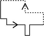
Figure 1: Illustration of the extra source terms, eq. (27), in the Dyson-Schwinger equations for a closed Wilson loop in the QEK model. The dashed line represents $W_{\rm open}$ while the solid line represents $W^{\prime}_{\rm open}$.

Such terms must all vanish for reduction to hold.

The argument that they do vanish proceeds in two steps HN ; GK ; Parisi-papers :

$$\int dp\,\,\left\langle W_{\rm open}\,\,W^{\prime}_{{\rm open}}\right\rangle_{p}\, = \int dp\,\,\left\langle W_{\rm open}\right\rangle_{p}\,\,\left\langle W^{\prime}_{{\rm open}}\right\rangle_{p}+\,O(1/N^{2})$$ (28)

$$\int dp\,\,\left\langle W_{\rm open}\right\rangle_{p}\,\,\left\langle W^{\prime}_{{\rm open}}\right\rangle_{p} = \int dp\,\,\left\langle W_{\rm open}\right\rangle_{p}\ \int dp^{\prime}\left\langle W^{\prime}_{{\rm open}}\right\rangle_{p^{\prime}}+\,O(1/N)\,.$$ (29)

The first step is large-$N$ factorization for a fixed set of $p$, valid to all orders in perturbation theory. The second step, which one might call “quenched factorization”, is special to the quenched theory. If it holds, then, due to the vanishing of quenched expectation values of open loops [as in Eq. (26)] the extra terms (27) in the loop equations do vanish in the large-$N$ limit.

We will argue in subsequent sections that the combination of eqs. (28) and (29) does not hold, most likely due to a failure of the latter equation. In order to understand what fails, we must first describe the argument for the correctness of these steps, and indeed why the quenching prescription is expected to reproduce the large-$N$ dynamics of $SU(N)$ lattice gauge theories.

The approach of Refs. BHN1 ; HN ; GK ; Parisi-papers ; DW provides an intuitive explanation of why large-$N$ quenched reduction works for a wide class of theories, albeit within perturbation theory. The idea relies on the fact that, in large-$N$ perturbation theory, only planar diagrams survive. In ‘t Hooft’s double-line notation each gluon line is replaced by two oppositely pointing lines that carry two indices $(a,b)$ with $a,b\in[1,N]$. In the reduced theory there is, initially, no momentum associated with a gluon “propagator”. The key point is then to associate a $d$-dimensional lattice momentum with each of the indices,

$$a\ \ \leftrightarrow\ \ p^{a}_{\mu}\,;\qquad p^{a}_{\mu}\in[0,2\pi)\,,$$ (30)

and to assign to the gluon with color indices $(a,b)$ the difference in the momenta associated with the two indices:

$$q^{ab}_{\mu}\equiv{\rm mod}\left(p^{a}_{\mu}-p^{b}_{\mu}\,,2\pi\right)\,\,.$$ (31)

It is easy to check that since one lets all $p^{a}_{\mu}$ take all values in $[0,2\pi)$, the momenta $q_{\mu}^{ab}$ of all gluons in any planar diagram will independently take values in the Brillouin zone, and will obey momentum conservation (modulo $2\pi$) at the vertices. This is impossible for non-planar diagrams, where some of the gluons carry the indices $(a,a)$ and so have $q^{aa}_{\mu}=0$.

The identification of Eq. (30) is necessary in order to embed space-time (or rather the first Brilluoin Zone of its momentum space) in color space, but it is only the first step. The next is to choose the action of the single-site model in such a way that the actual value of planar diagrams will be the same as that in the full gauge theory. In particular, they choose it such that the $(a,b)$ matrix element of the gluon propagator takes (in an appropriate gauge) the usual “$1/q^{2}$” form (or, more precisely, its lattice version) with $q$ indeed being the difference $p^{a}-p^{b}$. Vertices are similarly reproduced. In this way, for a given choice of color indices, one obtains the correct integrand of the corresponding infinite-volume large-$N$ Feynman diagram.

The application of the quenching prescription involves an important subtlety, which requires that additional constraints be placed on the single-site fields GK ; DW . The end result is that one arrives at precisely the QEK model, with the quenching prescription of Eqs. (18)–(21). The quantities $p_{\mu}^{a}$ are now viewed as (dimensionless) loop momenta. For example, perturbing around the classical vacuum of $V_{\mu}=\bm{1}$, yields the following two-point function for the fluctuating matrices $A^{ab}_{\mu}$

$$\langle A_{\mu}^{ab}A_{\nu}^{b^{\prime}a^{\prime}}\rangle_{p}=\delta_{\mu\nu}\delta_{aa^{\prime}}\delta_{bb^{\prime}}\frac{4}{\sum_{\nu}\sin^{2}\left(\frac{p_{\nu}^{a}-p_{\nu}^{b}}{2}\right)}\qquad(a\neq b),$$ (32)

which is the standard lattice result for the gluon propagator.

The final step in the quenching prescription of Ref. BHN1 ; GK ; Parisi-papers ; DW is to average over the momenta, as in eq. (21). The weight function should be manifestly $(Z_{N})^{d}$ invariant, and, as $N\to\infty$, force the momentum-components in each direction to densely cover the Brilluoin zone. An example for such a measure is that suggested in BHN2 :

$$\rho_{\rm VdM}(p)=\Delta^{2}(p)\,,$$ (33)

where the Vandermonde determinant is defined in Eq. (16). At large-$N$ the function $\rho_{\rm VdM}(p)$ forces the momenta to lie as far apart from each other as possible, and combined with the $SU(N)$ constraints (14), this requires the $p_{\mu}^{a}$ to be a permutation of the “clock” values,

$$P^{a}=\frac{2\pi}{N}\left(a-\frac{N+1}{2}\right)\,,\qquad a\in[1,N]\,.$$ (34)

The integral over $p$ then amounts to an average over permutations, independently for each direction. Since the momenta (34) are uniformly distributed, this gives a discrete approximation to the integration Eq. (21) over the infinite-volume momentum space. Thus as $N\to\infty$ one obtains, order by order in perturbation theory, the correct infinite-volume result for each Feynman diagram.

We can now give the argument of Refs. GK ; Parisi-papers for the crucial relation (29). Imagine evaluating the l.h.s. of Eq. (29) in perturbation theory, and focus on the contribution from planar diagrams with $(L+M)$-gluon loops, with $L$ loops coming from the expansion of $W_{\rm open}$, and the remaining $M$ loops from the expansion of $W^{\prime}_{\rm open}$. We can write this contribution as

$$\int dp\,\sum_{a_{1},a_{2},\dots,a_{L}\atop b_{1},b_{2},\dots,b_{M}}f(p_{a_{1}},p_{a_{2}},\dots,p_{a_{L}})\,g(p_{b_{1}},p_{b_{2}},\dots,p_{b_{M}}).$$ (35)

Here $f$ and $g$ denote the integrands of the planar diagrams contributing to the two Wilson loops, and $p_{a_{i}}$ and $p_{b_{i}}$ are the momenta that flow in these diagrams. If $(L+M)\ll N$ then a generic term in the double sum has all indices different, and for each such term the (normalized) integral over $p$ factorizes in the large-$N$ limit into the two integrals

$$\int dp\,f(p_{a_{1}},p_{a_{2}},\dots,p_{a_{L}})\,g(p_{b_{1}},p_{b_{2}},\dots,p_{b_{M}})=\int dp\,f(p_{a_{1}},p_{a_{2}},\dots,p_{a_{L}})\,\int dq\,g(q_{b_{1}},q_{b_{2}},\dots,q_{b_{M}})\,.$$ (36)

Here, for clarity, we changed the dummy integration variables $p_{b_{i}}$ to $q_{b_{i}}$. The last step is to sum Eq. (36) over all possible values of the indices $a_{i}$ and $b_{i}$, which gives the $L$-loop contribution to $\langle W_{\rm open}\rangle$ multiplied by the $M$-loop contribution to $\langle W^{\prime}_{\rm open}\rangle$. If this step is correct, we obtain the r.h.s. of Eq. (29).

This last step is only approximately correct for the following reason: Eq. (36) holds only if the indices $a_{1,\dots,L}$ are all different from the indices $b_{1,\dots,M}$, while in performing the final sum we ignore this restriction. At large-$N$, however, the effect of this “negligence” is only of $O(1/N)$—the fraction of terms with equal $a_{i}$ and $b_{i}$ indices. As a result one finds that to all orders in planar perturbation theory, quenched reduction holds at large-$N$. The fact that one ignores $O(1/N)$ terms here also explains why the quenched model has $O(1/N)$ rather than $O(1/N^{2})$ corrections.

III.4 Alternative choices of $\rho(p)$

The formulation of the QEK model provided by the approach of Refs. GK ; Parisi-papers shows that there is considerable freedom in choosing the weight function $\rho(p)$. The choice must simply turn the integrands of Feynman diagrams into their integrals as $N\to\infty$. The simplest choice is to use a uniform distribution: $\rho_{\rm uniform}(p)=1$ for all $N$. In practice, this can be implemented by Monte-Carlo—drawing $p$ randomly from a uniform distribution. Another choice, which we call $\rho_{\rm clock}(p)$, is to take the momenta to be a permutation of the clock values of eq. (34), even for finite $N$, and then average over permutations. This corresponds to setting

$$\rho_{\rm clock}(p)=\frac{1}{(N!)^{4}}\left(\prod_{\nu}\sum_{\sigma_{\nu}}\right)\left\{\prod_{\mu,a}\delta(p_{\mu}^{a}-P^{\sigma_{\mu}(a)})\right\}\,,$$ (37)

where the $\sigma_{\mu}(a)$ are permutations of the color indices. With this choice, which we use extensively below, the center-symmetry-breaking order parameters ${\text{t}r}\,\,U_{\mu}^{p}$ (for $p\neq 0\ {\rm mod}\ N$) vanish prior to the average over permutations. This choice also has a simple physical interpretation. The discrete $p_{\mu}$ are those that one would obtain if one had a lattice with $N$ sites in each direction, with periodic/antiperiodic boundary conditions for $N$ odd/even. After averaging over permutations one obtains the result of the Feynman diagram on a lattice of physical volume $(Na_{\rm lat})^{d}$, where $a_{\rm lat}$ is the lattice spacing.

It is further argued in Ref. GK ; Parisi-papers that the integral over momenta (or sum over permutations) becomes unnecessary as $N\to\infty$. This is because Eq. (31) implies that the sum over the color indices in each color loop becomes an integral over the corresponding Brillouin zone. Thus a single choice of randomly chosen momenta, or a single set of randomly chosen permutations of clock momenta, should, in principle, be sufficient. In practice, for finite $N$, it may be preferable to include an average over such choices.

The final choice of $\rho(p)$ we consider is that suggested in GK and analyzed by Bars in Bars . It applies only when $N=K^{d}$, where $K$ is an integer. In this case $\rho(p)$ is a product of delta-functions such that each value of the color index is associated with a different $d$-dimensional momentum lying on a $K^{d}$ latticization of the Brillouin zone (BZ). In four dimensions one has

$$\!\!\!\!\left\{p_{1}^{a},\,p_{2}^{a},\,p_{3}^{a},\,p_{4}^{a}\right\}=$$ (38)

$$\!\!\!\!\!\!\!\frac{2\pi}{K}\left\{{\rm mod}\left(a\!-\!1,K\right),{\rm mod}\left(\left[\frac{a\!-\!1}{K}\right],K\right),{\rm mod}\left(\left[\frac{a\!-\!1}{K^{2}}\right],K\right),{\rm mod}\left(\left[\frac{a\!-\!1}{K^{3}}\right],K\right)\right\},$$

where $[x]$ indicates the integer part. We shall henceforth denote this choice by “BZ”. As an example, consider the two-dimensional case with $N=16$ (so $K=4$). We divide the Brillouin zone into sixteen boxes, and set the sixteen momenta $p^{a}$ to lie at their centers, as shown in Fig. 2.

Figure 2: A two-dimensional example of the embedding suggested in Refs. GK ; Bars of the color indices in the Brilluoin zone for $N=16$.

For $\rho(p)=\rho_{BZ}(p)$, the momenta are those for a physical volume $(Ka_{\rm lat})^{d}=N(a_{\rm lat}^{d})$, which is much smaller than that obtained using the clock momenta. The advantage of using $p=p_{\rm BZ}$ is that one obtains a uniform distribution over the Brillouin zone from a single set of momenta, already at finite $N$.

The general discussion of the realization of center and reflection symmetries given in Section III.2 must be modified for $\rho_{\rm clock}$ and $\rho_{\rm BZ}$. These symmetries can now be realized by a transformation on the $V_{\mu}$. Consider first the clock momenta. There is then an $SU(N)$ matrix $S$, such that, when $V_{\mu}\to SV_{\mu}$,

$$U_{\mu}=V_{\mu}^{\dagger}\Lambda_{\mu}V_{\mu}\to V_{\mu}^{\dagger}S^{\dagger}\Lambda_{\mu}SV_{\mu}=V_{\mu}^{\dagger}(\Lambda_{\mu}z_{\mu})V_{\mu}=U_{\mu}z_{\mu}\,.$$ (39)

This is possible because, first, up to an overall phase, the elements of $\Lambda_{\mu}$ are a permutation of the N’th roots of unity (so that multiplication by $z_{\mu}$ corresponds to a permutation of these elements) and second the eigenvalues of $\Lambda_{\mu}$ can be arbitrarily permuted by conjugation by $SU(N)$ matrices (as will be discussed in detail in the subsequent section). The reflection transformations also correspond to permutations of the eigenvalues, and can be accomplished by different choices of $S$.

The situation is slightly different for $\rho_{\rm BZ}$. Here the quenched theory only realizes a $(Z_{K})^{d}$ subgroup of the center symmetry, because only such transformations correspond to a permutation of the momenta. The reflection transformations are also realized by permutations.

IV Breakdown of quenched reduction - analytic considerations

As explained in the previous section, the validity of quenching is predicated on the momenta being fixed by hand, independently in each direction, and then integrated over with a suitable weight function. This is possible in perturbation theory. When one does a non-perturbative calculation, however, the values of $p$ are not completely fixed, and their distribution is thus determined in part by dynamics. In other words, they are incompletely quenched. We argue in this section that, at least in the weak coupling limit $b\to\infty$, the dynamics is likely to choose a ground state in which this incomplete quenching invalidates reduction in perturbation theory, and also invalidates the key relations (28-29). If this persists beyond perturbation theory, then reduction fails. Our numerical results, obtained for finite $b$, suggest that this is indeed what occurs.

The key observation is simply stated. The “fixed” momenta can be dynamically permuted, independently in each direction, by fluctuations in the $V_{\mu}$. These innocent-sounding permutations lead, in general, to a different free energy, and the dynamics chooses the permutation(s) with the lowest free energy. The $p$’s that one puts in by hand are different, in general, from those chosen by the dynamics, and the latter are not uniformly distributed in the Brillouin Zone. Thus, the sum over color indices does not lead to a uniform integration over the Brillouin zone, and the agreement with infinite-volume perturbation theory fails.

The presence of permutations in the dynamics has long been known, and was stressed particularly in Refs. Neuberger-permutations ; Parsons and KNN . To our knowledge, however, the implications for the validity of reduction have not previously been noted.

IV.1 “Momentum locking” at weak coupling

Permutations are generated by transpositions, in which $p_{\mu}^{a}\leftrightarrow p_{\mu}^{b}$ for one pair $(ab)$ and one choice of $\mu$. Transpositions can be accomplished, for example, by multiplying $V_{\mu}$ from the left by the $SU(N)$ matrices $V^{(ab)}(\phi)$, which are the identity aside from

$$\left(V^{(ab)}(\phi)\right)_{(ab)\ {\rm block}}=e^{i\phi\sigma_{1}}\,.$$ (40)

As $\phi$ runs from $0$ to $\pi/2$, $V_{\mu}^{\dagger}\Lambda_{\mu}V_{\mu}$ changes to $V_{\mu}^{\dagger}\Lambda^{\prime}_{\mu}V_{\mu}$, where $\Lambda^{\prime}_{\mu}$ differs from $\Lambda_{\mu}$ in having the $a$’th and $b$’th momenta permuted. Since it is possible to reach any permutation by a sequence of transpositions, an ergodic simulation will pass through all possible permutations of the input momenta. The question then is which of these permutations has the smallest free energy. Only if they are equally likely will the quenched model work as desired.

We can calculate the relative free energies in the weak-coupling limit. First we describe the energy (i.e. action) “landscape”. The minimum energy states, after appropriate gauge fixing, have $V_{\mu}={\bf 1}$ and the momenta in any permutation of their input values. This is because the plaquette is unity for any choice of diagonal $\Lambda$’s. If the momenta are non-degenerate, there are in fact $(N!)^{d-1}$ different “vacua” (one factor of $N!$ being removed using a gauge transformation Eq. (3) to keep $\Lambda_{\mu=1}$ in its input order). These vacua are connected by the $V^{(ab)}(\phi)$, with the energy barrier (at $\phi=\pi/4$) being Neuberger-permutations ; Parsons

$$-\Delta S_{\rm QEK}=8Nb\,\sin^{2}(\Delta p_{\mu}^{ab}/2)\sum_{\nu\neq\mu}\sin^{2}(\Delta p_{\nu}^{ab}/2)\,.$$ (41)

Here the transposition is being done on $\Lambda_{\mu}$, and $\Delta p_{\mu}^{ab}=p_{\mu}^{a}-p_{\mu}^{b}$. Generically, all the $\Delta p$ are of $O(1)$, and the barrier height then grows as $N$. There will always be some $(ab)$ pairs, however, that have $\Delta p=O(1/N)$, and for these the energy barrier vanishes with increasing $N$. Nevertheless, for fixed $N$, as $b\to\infty$, these barriers too become infinitely high.

Thus, in the weak-coupling limit, and assuming non-degenerate momenta, one can treat the system as a collection of independent vacua with $V_{\mu}$ fluctuating around unity in each. At leading order the free energy in each vacuum is, up to an irrelevant constant, BHN1 ; MK

$$-\ln Z(p) = F_{\rm EK}(p)+F_{2}(p)\,,$$ (42)

$$F_{\rm EK}(p) = (d-2)\sum_{a<b}\log\left(\sum_{\mu}\sin^{2}[\Delta p_{\mu}^{ab}/2]\right)$$ (43)

$$F_{2}(p) = -\ln\Delta^{2}(p)\,.$$ (44)

This is just a repetition of the result already quoted in Eq. (17), taking into account the difference in the definitions of $Z(p)$ and $Z_{\rm EK}(p)$. Since $\Delta^{2}(p)$ is the same for all permutations, it is only $F_{\rm EK}(p)$ which distinguishes between them. The argument of the logarithm in $F_{\rm EK}(p)$ is just the lattice gluon propagator, and the overall factor $d-2$ is the number of transverse gluons. The key observation is simply that $F_{\rm EK}(p)$ depends on the permutation of the momenta. To see this qualitatively, note that, because the logarithm is a concave function, $F_{\rm EK}(p)$ is minimized by choosing permutations in which there are values of $(ab)$ for which $\Delta p_{\mu}^{ab}$ is simultaneously small in all directions. In other words, one lowers the free energy by aligning, or “locking”, the momenta in different directions. The gain one makes by locking the small momenta outweighs the loss incurred by locking large momenta.

We note that it is the same free energy $F_{\rm EK}(p)$ that causes the spontaneous breakdown of the center symmetry in the EK model. In that case the momenta are fully dynamical, and $F_{\rm EK}(p)$ causes them to be equal, as discussed in Sec. II. This collapse is prevented by quenching, but quenching, which acts independently in each direction, does not prevent correlations between momenta in different directions, such as that induced by “locking”.

We have numerically checked the argument that minimizing $F_{\rm EK}(p)$ leads to locking in the following way. We considered the clock momenta, and evaluated $F_{\rm EK}$ of Eq. (43) for many random permutations of the momenta. What we find is that the vast majority of permutations have a free energy larger by $O(N^{2})$ than that for the completely locked case. (An example of this result is given below in Fig. 3.) Thus as $b\to\infty$ at fixed $N$, the completely locked vacua dominate. As noted in Sec. III.4, the $(Z_{N})^{d}$ transformations and reflections form a subset of the permutations, and for these the free-energy is invariant. Thus there are $(2N)^{d-1}$ degenerate vacua of the locked type, whereas for general (non-clock) momenta we expect only a single vacuum.

In preparation for the numerical study, we now discuss quantities that can be used to discern the predicted locking of momenta. As we will explain, for the clock momenta these are appropriately called order parameters, although for general $\rho(p)$ they are not. The simplest choices are the expectation values of the $d(d-1)$ open loops

$$M_{\mu,\nu}\equiv{\text{t}r}\,(U_{\mu}U_{\nu})/N\quad{\rm and}\quad M_{\mu,-\nu}\equiv{\text{t}r}\,(U_{\mu}U_{\nu}^{\dagger})/N\quad(\mu>\nu)\,,$$ (45)

which are sensitive to correlations between gauge fields in different directions. The utility of these quantities is particularly clear for the clock momenta, for which one of the permutations leads to the $\Lambda_{\mu}$ being equal in all directions. Then, if $V_{\mu}\to 1$, half of the $|M_{\mu,\nu}|$ equal unity ($M_{\mu,-\nu}=1$), while the other half vanish ($M_{\mu,\nu}=0$). The same absolute values of the $M_{\mu,\nu}$ hold for the other locked vacua obtained by acting with $(Z_{N})^{d}$ transformations, while $M_{\mu,-\nu}$ and $M_{\mu,\nu}$ switch roles under reflections. This suggests using the combined quantity

$$M=\sum_{\mu<\nu}\left(|M_{\mu,\nu}|+|M_{\mu,-\nu}|\right),$$ (46)

as a signal for locking. We use both $M$ and the individual $M_{\mu\nu}$ in our numerical study.

To illustrate the utility of $M$, we present in Fig. 3 a scatter plot of the normalized free energy versus $M$ for a large set of randomly chosen permutations of the clock momenta and with $V_{\mu}=\bm{1}$. We include the locked vacua by hand, since they are not among those chosen randomly. The figure indicates that the locked configurations have free energies that are at least of $O(N^{2})$ smaller than those of the “unlocked” configurations, and have significantly larger values of $M$. Taking the results at face value, one might be concerned that the number of unlocked vacua might overcome their higher free-energy. However their entropy factor is $\ln N!\sim N\ln N$, which is thus smaller than the free-energy difference of $O(N^{2})$ or greater. Nevertheless, this plot does lead one to expect that, for finite $N$, a range of “partially unlocked” states (present in the figure only for $N=10$) will be populated.

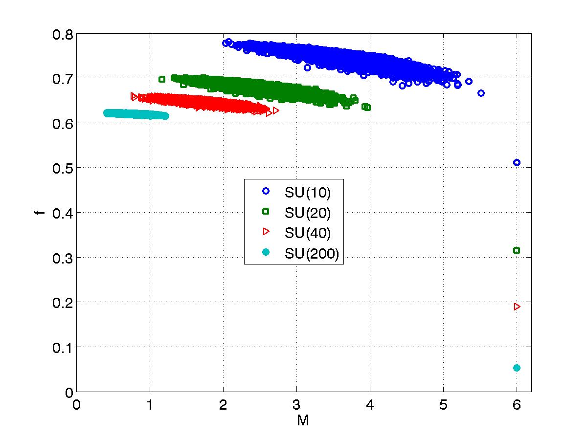
Figure 3: The dependence of $f=F_{\rm EK}(p)/((d-2)N(N-1)/2)$ on the combined order parameter $M$ for random permutations of the clock momenta. Results are for $d=4$ and $N=10,20,40,200$. The fully locked points with $M=6$ are included by hand. There are also partially unlocked states which, for each $N$, interpolate between the mass of unlocked states and the locked ones. These do not appear in the random sampling except for $N=10$.

In Section V we use these order parameters and other numerical evidence to argue that locking does occur also nonperturbatively. For the remainder of this section we discuss in more detail how locking leads to a failure of reduction. In particular, we explain why the previous arguments, summarized in Section III.3, do not hold.

IV.2 Implications of momentum locking for large-$N$ reduction

In this section we first focus on the case of the clock momenta, and then return to other choices. As noted above, the quenched average in this case is just an average over permutations of the momenta. But we now understand that the non-perturbative QEK model automatically includes this sum over permutations—it is self-averaging. Thus, in principle, the additional quenched average is unnecessary. We also know, however, that the permutations are included with different relative weights—this is manifest in the weak coupling free-energy landscape of Fig. 3, and there is no reason to expect equality for other couplings. Regardless of the details, the mere fact that the weights are different implies that the integrations over momentum space that are induced by the sums over color indices are not uniform. This is sufficient to invalidate reduction —the momentum integrations in the reduced and infinite-volume cases are different. The case of complete locking provides an extreme example: the momentum of each gluon then has the same component, $\Delta p_{\mu}^{ab}$, in each direction, and the integration over the $d$-dimensional Brillouin zone collapses to an integration along the 1-dimensional body diagonal.

The argument for reduction based on the loop equations also fails, because one or other of the key steps, eqs. (28) and (29), does not hold. To see how this works, we write out these relations for the case that $W_{\rm open}=M_{\mu,\nu}$ and $W^{\prime}_{{\rm open}}=M_{\mu,\nu}^{*}$:

$$\int dp\,\,\left\langle M_{\mu,\nu}\,\,M_{\mu,\nu}^{*}\right\rangle_{p}\, = \int dp\,\,\left\langle M_{\mu,\nu}\right\rangle_{p}\,\,\left\langle M_{\mu,\nu}^{*}\right\rangle_{p}+O(1/N^{2})$$ (47)

$$\int dp\,\,\left\langle M_{\mu,\nu}\right\rangle_{p}\,\,\left\langle M_{\mu,\nu}^{*}\right\rangle_{p} = \int dp\,\,\left\langle M_{\mu,\nu}\right\rangle_{p}\int dp^{\prime}\left\langle M^{\star}_{\mu,\nu}\right\rangle_{p^{\prime}}+O(1/N).$$ (48)

We now argue that, if locking occurs, then, for some $\mu$ and $\nu$, the following two statements are correct :

1. The r.h.s. of Eq. (48) is of $O(1/N)$.

2. The l.h.s. of Eq. (47) is of $O(1)$.

Thus one or both of the relations must be wrong. The numerical evidence of Section V suggests that it is the second relation, Eq. (48), which fails.

It is easy to see that statement (I) is correct regardless of the choice of $\rho(p)$. This is due to the center symmetry (24), under which

$$\left\langle M_{\mu,\nu}\right\rangle_{p}\longrightarrow\left\langle M_{\mu,\nu}\right\rangle_{p+{2\pi n}/{N}}=\left\langle M_{\mu,\nu}\right\rangle_{p}\,e^{2\pi i(n_{\mu}+n_{\nu})/N},$$ (49)

Since the measure $dp$ is unchanged when $p\to p+2\pi n/N$, the phase factors will cause $\int dp\left\langle M_{\mu,\nu}\right\rangle_{p}$ to vanish. For the clock momenta the situation can be slightly different. There, self-averaging may take place, and this means that the momenta that contribute to $\left\langle M_{\mu,\nu}\right\rangle_{p}$ are all those related to $p$ by permutations. These include also the momenta $p^{a}_{\mu}+2\pi n_{\mu}/N$ with $n_{\mu}$ integer, and so $\left\langle M_{\mu,\nu}\right\rangle_{p}\sim\sum_{n_{\mu},n_{\nu}}e^{2\pi i(n_{\mu}+n_{\nu})}=0$. Consequently we see that self-averaging in the clock momenta case makes statement (I) correct even without the integrations.

To see why statement (II) is correct note that the locking means that some of the $|M_{\mu,\nu}|$ will have $O(1)$ values. In contrast to the integrands of Eq. (48), the integrand here, $M_{\mu,\nu}M_{\mu,\nu}^{*}=|M_{\mu,\nu}|^{2}$, is invariant under the center symmetry, and thus maintains its $O(1)$ value even after integration.

Which of the two Equations (47) and (48) fails? This depends on the nature of the dynamics. If the self-averaging occurs, then the second step, which for clock momenta is simply

$$\left\langle M_{\mu,\nu}\right\rangle_{p}\,\,\left\langle M_{\mu,\nu}^{*}\right\rangle_{p}=\left\langle M_{\mu,\nu}\right\rangle_{p}\left\langle M^{\star}_{\mu,\nu}\right\rangle_{p^{\prime}}\,,$$ (50)

is trivially valid, and it is the first step which fails. This breakdown of large-$N$ factorization is then an example of the breakdown of cluster decomposition due the presence of multiple vacua —all those related by the center and reflection symmetry.

The other possibility is spontaneous symmetry breaking (SSB) of the center symmetry, in which the system gets stuck in the vicinity of one of the locked vacua. We recall that $Z(p)$ itself is $(Z_{N})^{d}$ symmetric with clock momenta, so there is a symmetry to break. Furthermore, despite the fact that the QEK model has zero volume, SSB is possible when $N\to\infty$ because there are then an infinite number of degrees of freedom. The $\left\langle M_{\mu,\nu}\right\rangle_{p}$ (or, indeed, the quenched expectation values of any open loops) are order parameters—non-vanishing values indicate SSB. If SSB takes place then, by definition, self-averaging no longer occurs, and vacuum expectation values of open loops vanish only if we explicitly average over the input permutations. If the input permutation is changed by a center transformation, then, since the dynamics is $(Z_{N})^{d}$ invariant, the vacuum that is selected will also be changed by the same transformation. In this possibility, factorization, Eq. (47), holds, because fluctuations about the single vacuum are suppressed as $N\to\infty$. It is the second step, Eq. (48), that fails. On the l.h.s. the same vacua are selected in the two quenched expectation values, because the same input momenta are used, while on the r.h.s. different vacua are, in general, selected. Thus the l.h.s. will be of $O(1)$ for all input $p$, while the first term on the r.h.s. will average to zero. Thus what we call quenched factorization fails.

We discuss which of the two possibilities—self-averaging or SSB—is expected to occur in the next subsection. Regardless of which occurs, however, the key point is that the combination of the relations (47-48) fails, either invalidating cluster decomposition or breaking the center symmetry, and thus large-$N$ reduction fails. Furthermore, one can numerically test for this by calculating the l.h.s. of (47) and determining whether it falls as $1/N$ (as required for reduction) or tends to a constant as $N\to\infty$ (reduction fails).

We now consider the uniform weight function, $\rho(p)=1$. In this case $Z(p)$ is not center-symmetric and the $M_{\mu,\nu}$ are not order parameters. Nevertheless, if locking occurs, we expect something similar to SSB to take place. For a random input choice of $p$, we expect the system to sample the space of permutations, until it finds that with the smallest free energy. Note that none of the permutations will be related by center or reflection symmetries, so all are expected to have different free energies. In this picture, the system ends up fluctuating in the vicinity of a particular permutation. If the weak-coupling free energy is any guide, the chosen permutation will be such that if, for a given pair of indices $(a,b)$, the difference $\Delta p_{\mu}^{ab}$ is small for one value of $\mu$, then it will also be small for all other values of $\mu$. In other words the chosen momenta will be partially locked. Thus, even though the input momenta are uniformly distributed in the BZ, those chosen dynamically are not, and planar perturbation theory is not correctly reproduced.

The expected partial locking implies that, for most input $p$, some of the $M_{\mu,\nu}$ will fluctuate around complex values with magnitudes of $O(1)$. If so, this invalidates the quenched factorization of Eq. (48), because the l.h.s. averages to an $O(1)$ value, while the $p$-integrals on the r.h.s. implement the center symmetry and cause the averages to vanish. This picture is confirmed by our numerical findings in Section V.

For $\rho_{\rm BZ}$ the situation is similar to that for $\rho_{\rm clock}$. There are multiple locked vacua related by the center and reflection symmetries, and locking invalidates reduction. The difference is that it is only the $(Z_{K})^{d}$ subgroup of the full center symmetry which is realized, where $K=N^{1/d}$. To make clear how the presence of permutations in the dynamics unravels the carefully chosen coverage of the BZ, we can refer to the simple example in Fig. 2. Permuting the momentum components in the “1” direction as, for example, $p_{1}^{a}\leftrightarrow p_{1}^{b}$ for $(ab)=(25)$, moves the two momenta in the “boxes” labeled 2 and 5 in the Figure into those labeled by 1 and 6, where the momenta are locked. Similarly, all other off-diagonal pairs can be moved by permutations onto the diagonal. Thus if the free-energy favors locking, as the weak-coupling argument implies, then the momenta chosen by the simulation will lie on the one-dimensional diagonal of the BZ.

Finally, we briefly discuss the choice $\rho(p)=\rho_{\rm VdM}(p)$ of Eq. (33). This is in some sense intermediate between the clock and uniform choices. On the one hand, any value of $p$ is possible with $\rho_{\rm VdM}(p)$, while, on the other, the large-$N$ limit of $\rho_{\rm VdM}(p)$ is $\rho_{\rm clock}(p)$. Thus we expect locking or partial-locking for $\rho_{\rm VdM}$, and this is indeed what we find numerically.

IV.3 Expected size of fluctuations

In this subsection we address the question of whether, for the clock momenta, we expect the theory to exhibit SSB or not. We are interested in this question for fixed $b$ and $N\to\infty$. The weak-coupling result of Eq. (43) provides a guide to the free-energy landscape, and suggests that the dominant states correspond to fluctuations about the locked vacua. As in any statistical mechanical system, the issue is whether the fluctuations are large enough to cause the theory to move from one locked vacuum to others related by symmetry transformations. In infinite volume, we know from the Mermin-Wagner-Coleman theorem MWC that for $d>2$ the fluctuations are not IR divergent and SSB is possible, while for $d\leq 2$ it is not. The question is how this result translates to the QEK model where the spatial volume is embedded in the color space.

To get a rough idea of what happens, imagine that we are in a completely locked vacuum. A measure of the fluctuations in the (normalized) traces of open Wilson loops (such as the $M_{\mu,\nu}$) is given by the “tadpole” graph

$$T\equiv\frac{g^{2}}{N}\sum_{a\neq b}\langle A_{\mu}^{ab}A_{\mu}^{ba}\rangle_{p}=\frac{g^{2}}{N}\sum_{a\neq b}\frac{4}{\sum_{\nu}\sin^{2}(\Delta p_{\nu}^{ab}/2)}\,,$$ (51)

where $\mu$ is fixed, and we have used Eq. (32). The $g^{2}$ comes from expanding the $U_{\mu}$, and the $1/N$ from the normalized trace. Note that since we are doing perturbation theory we can really fix the momenta, and we are taking $p$ to be locked. This means that $|\Delta p_{\nu}^{ab}|=|P^{a}-P^{b}|$ is independent of $\nu$, and the tadpole can be rewritten as

$$T_{\rm locked}=\frac{g^{2}}{N}\sum_{a\neq b}\frac{1}{\sin^{2}([P^{a}-P^{b}]/2)}=1/b\int_{c/N}^{\pi}\frac{dq}{\pi}\frac{1}{\sin^{2}(q/2)}+O(1/N)\,.$$ (52)

As $N\to\infty$, the sum has gone over to an integral, but the integral is over a one-dimensional momentum space, and is thus IR divergent. The cut-off $c/N$ (with $c$ a constant that could be determined by a more complete analysis) arises from fact that the original sum, Eq. (51), has a minimum $\Delta p$ of $O(1/N)$. The IR divergence implies that

$$T_{\rm locked}\propto N/b\,[1+O(1/N)]$$ (53)

so that the fluctuations about the locked vacua diverge as $N\to\infty$ for fixed $b$.

These divergences can be anticipated from the result for the maximum energy barrier $\Delta S_{\rm QEK}$ (see Eqs. (40)-(41)) that exists between two configurations related to each other by the permutation $p^{a}_{\mu}\leftrightarrow p_{\mu}^{b}$. Denoting $\Delta p_{\mu}^{ab}\equiv p^{a}_{\mu}-p_{\mu}^{b}$, we see that if $\Delta p_{\mu}^{ab}=O(1/N)$ and $\Delta p^{ab}_{\nu}\sim O(1)$, then $|\Delta S_{\rm QEK}|\sim b/N$, and fluctuations in the direction parameterized by the $SU(N)$ matrix (40) overcome the barrier when $N$ is large enough that $b/N<O(1)$. For locked vacua with $\Delta p_{\mu}=O(1/N)$ in all directions, the barrier is even lower, $|\Delta S_{\rm QEK}|\sim b/N^{3}$. The Gaussian terms in the action for these “flat” directions is small relative to higher-order terms, and ignoring the latter in the tadpole calculation leads to the apparent IR problem.

It is, in fact, the more severe $b/N^{3}$ divergence which leads to $T_{\rm locked}\propto N$. One can see this by noting that for a random permutation of the clock momenta $T\sim\int d^{4}q/q^{2}$ in the IR, and this is convergent. This is despite the fact that there are the flat directions with $|\Delta S_{\rm QEK}|\sim b/N$.

The upshot of this discussion is that we cannot quantitatively trust the weak-coupling calculation of $T$ for the locked vacua if $N\to\infty$ at fixed $b$. How does this affect the free-energy $F_{EK}(p)$ which we discussed above for the locked vacua? It follows from Eq. (43) that

$$F_{\rm EK}(p_{\rm locked})\sim N^{2}\int_{c/N}^{O(1)}dq\,q\log(q)\sim O(N^{2})+O(N\log N)\,,$$ (54)

and so the leading order term is IR safe, while the subleading term cannot be trusted in a Gaussian analysis. Since our previous discussion was based on the leading $O(N^{2})$ term, it remains valid.

Returning to the issue of SSB, we need to know whether the large-$N$ divergence of $T_{\rm locked}$ implies that the system will fluctuate into nearby locked vacua (which have momenta differing by center-transformations or reflections). We know that there will be large fluctuations in the directions given by transpositions between close momenta, for these are the source of the IR divergence. Thus to address the question we proceed as follows. It is possible to move from one locked vacuum to another by stringing together a sequence of transpositions involving nearby $p$’s (i.e. with $\Delta p$ always of $O(1/N)$). As we proceed along such a string, the momenta become partially unlocked, and the energy barriers to transpositions increase from of $O(1/N^{3})$ to of $O(1/N)$. Nevertheless, they all still vanish as $N\to\infty$, so there is a vanishing energy barrier between locked vacua. What matters, however, is whether there is a free-energy barrier. We can investigate this using the weak-coupling result, evaluating Eq. (43) numerically for each momenta along the path.

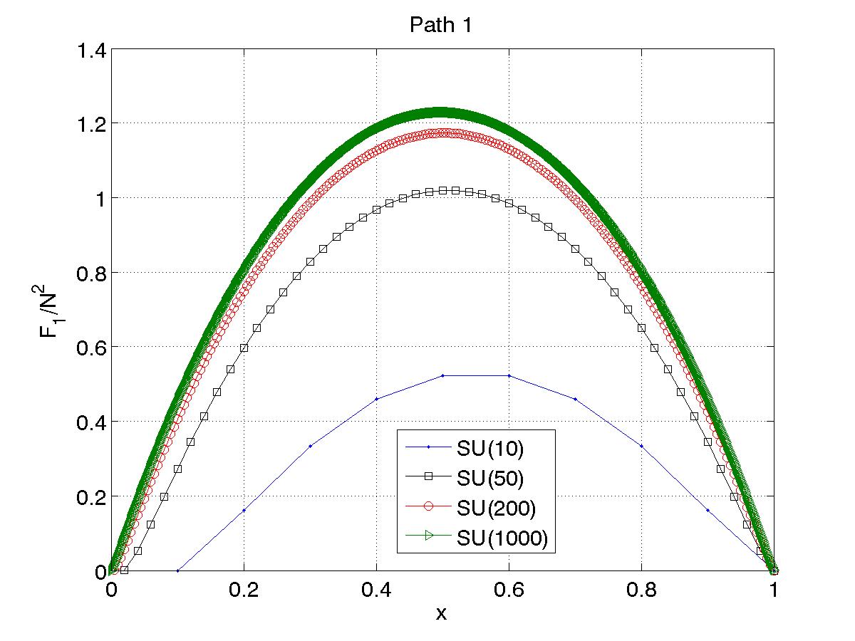
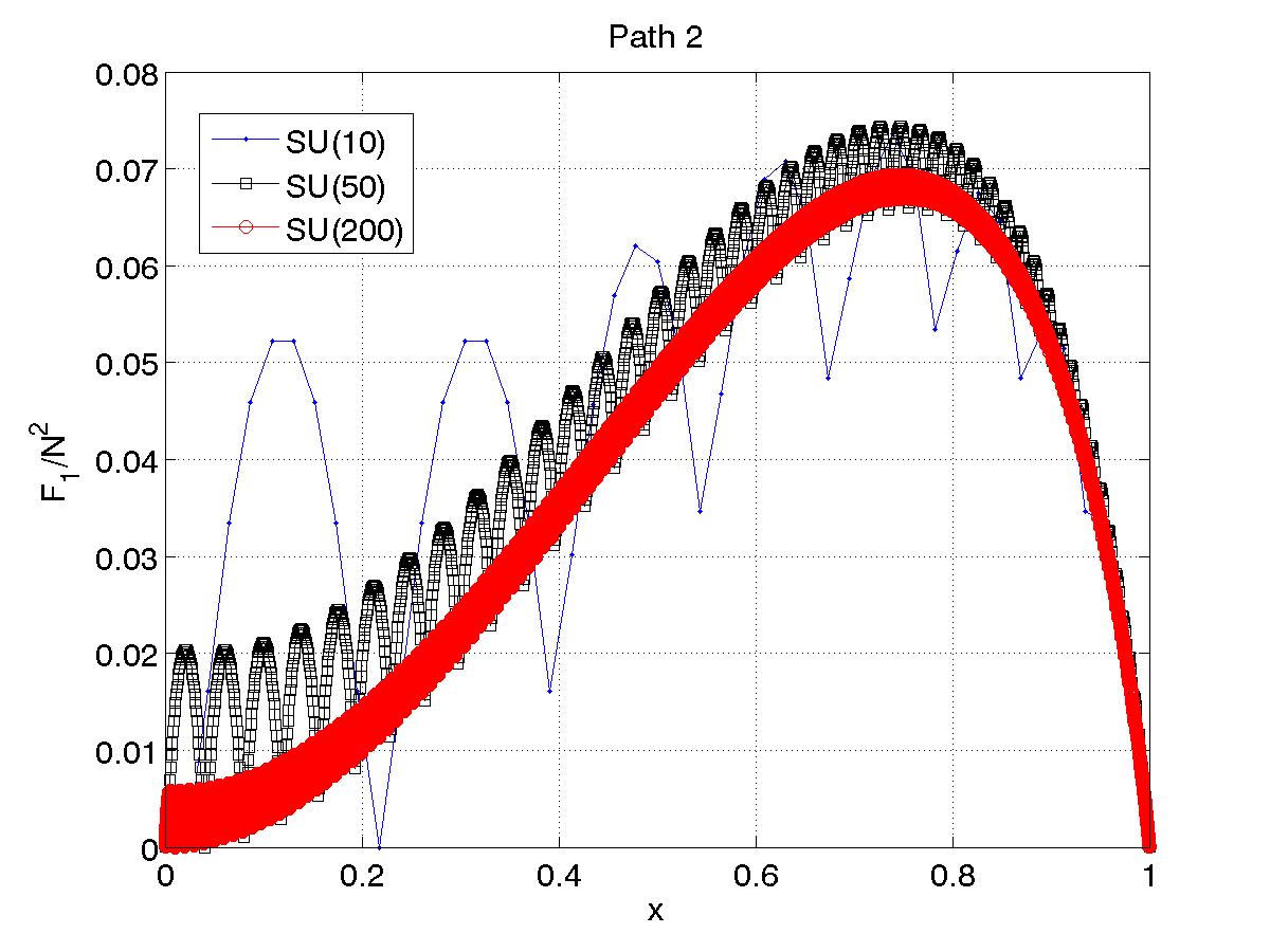
Figure 4: The free energy $F_{\rm EK}(p)/(d-2)$, divided by $N$ (left panel) or $N^{2}$ (right panel), along the two paths between locked vacua described in the text. Results are for $d=4$ and $N=10$, $50$, $200$ and $1000$. The horizontal axis gives the fraction of the total transpositions required, with the starting point being plotted at position $1/N$ (left panel) and $2/[N(N-1)+1]$ (right panel). The left panel is for path 1 (vacua related by center-symmetry), the right panel for path 2 (vacua related by a reflection).

We have considered two types of path. Both begin from a locked state in which $U_{\mu}=\Lambda_{1}$ for all $\mu$, where $(\Lambda_{1})_{aa}=\exp(iP^{a})$, with the $P^{a}$ given in Eq. (34). Thus, for example, $M_{\mu,\nu}=0$ and $M_{\mu,-\nu}=1$. Path 1 arrives at a state with $U_{1}=U_{3}=U_{4}$ unchanged and $U_{2}=U_{1}e^{-2\pi i/N}$, so that $M_{12}=0$, $M_{1,-2}=e^{+2\pi i/N}$, etc.. The path is made of a series of $N-1$ transpositions between adjacent indices, for each of which $|\Delta p|$ takes its minimal value of $2\pi/N$. The paths we use are exemplified by the following sequence for $N=6$ (which shows the ordering of the momenta $P^{a}$, $a\in[1,6]$, along the diagonal of $U_{2}$)

$$123456\to 213465\to 312564\to 412356\to 512346\to 612345\,.$$ (55)

In contrast, path 2 takes us to a vacuum with $U_{1}=U_{3}=U_{4}=\Lambda_{1}$ and $U_{2}=\Lambda_{1}^{\dagger}$, for which $M_{1,2}=1$ and $M_{1,-2}=0$. This can be achieved with transpositions alone along a more complicated path of length $N(N-1)/2$, that for $N=6$ would be the string of transpositions in Eq. (55), followed by

$$612345 \to 6213465\to 631245\to 641235\to 651234\to 652134\to 653124\to 654123\to$$ (56)

$$654213 \to 654312\to 654321.$$

We show the results in Fig. 4. We find that, for path 1, the free energy barrier $\Delta F$ scales asymptotically with $N$, while for path 2 it scales with $N^{2}$. Since we know from above that the $O(N^{2})$ part of the free energy is IR safe, we conclude that fluctuations along path 2 are certainly suppressed. For path 1 the situation is more subtle, as we now discuss.

The issue for path 1 is whether the leading contribution to $\Delta F$, which we see to be of $O(N)$, is IR safe, given that $F$ itself is untrustworthy at this order. The numerical results themselves suggest that the $N\log N$ terms cancel in $\Delta F$, but it would require a more detailed analytic analysis to demonstrate that this cancellation of untrustworthy terms is itself trustworthy. Thus the most conservative conclusion is that we do not know whether the barrier path 1 grows with $N$ and suppresses fluctuations. Other uncertainties in this analysis are that we have not investigated all paths, nor accounted for a possible entropy factor involving the number of paths, and finally that it is based on the leading term in the weak-coupling analysis. Thus to learn about the extent of locking, and the possibility of SSB, we must study the QEK model non-perturbatively, and to this we now turn.

V Non-perturbative Lattice Study

In this section we present our numerical results for the QEK model. In Sec. V.1 we briefly describe the methodology, focusing on an explanation of the two strategies we adopt to perform the quenched average: self-averaging and explicit averaging. In Sec. V.2 we map the phase structure as a function of the bare coupling, $b$, using measurements of the plaquette and the order parameters $M_{\mu,\nu}$. These results lead us to investigate various features of the model in more detail. In Sec. V.3 we describe results from high-precision measurements of the plaquette. This allows us to study the dependence of the results on the calculational strategy and on the choice of the weight function $\rho(p)$ (defined in Section III.3). We present similar measurements for $M_{\mu,\nu}$ in Sec. V.4 and use them to understand the structure of the vacua of the QEK model. Finally, in Sec. V.5, we analyze a “strong-to-weak” transition that occurs in the model, using an adaptation of the Wang-Landau algorithm WL to perform a precise measurement of the coupling $b_{t}$ at which it occurs.

V.1 Methodology

The QEK model has been defined above in eqs. (18)-(21). The ingredients for a simulation are a weight function for the momenta, $\rho(p)$, and the coupling $b$ in the quenched action, eq. (19). Specifically one is instructed to draw momenta weighted by $\rho(p)$, construct the diagonal eigenvalue matrices $\Lambda_{\mu}$ using eq. (13), and then do a Monte-Carlo average over the $SU(N)$ matrices $V_{\mu}$ for fixed $\Lambda_{\mu}$. Observables involving gauge links, such as the plaquette, can then be reconstructed using the definition $U_{\mu}=V_{\mu}^{\dagger}\Lambda_{\mu}V_{\mu}$.

As noted above, we consider four choices of weight function: uniform ($\rho_{\rm uniform}(p)=1$), clock [defined in eq. (37)], Vandermonde [defined in eq. (33)], and BZ [defined above eq. (38)]. It is straightforward to draw momenta from the first three of these distributions, while there is only a single choice for the BZ distribution.

The Monte-Carlo integration over the $V_{\mu}$ is non-standard because the action (19) is quartic in each of these matrices, so that a simple heat-bath algorithm cannot be used. Instead, we use the following three approaches.

1. A straightforward (and slow) Metropolis algorithm using the original action, updating all of the $SU(2)$ subgroups of each $V_{\mu}$ in turn;

2. A faster Metropolis algorithm, using a Gaussian auxiliary field to reduce the action to quadratic order in the $V_{\mu}$ FabriciusHahn . We again update $SU(2)$ subgroups of $V_{\mu}$ in turn.

3. A combination of a Cabibbo-Marinari heat-bath (again applied in turn to $SU(2)$ subgroups) and various type of over-relaxations (both $SU(2)$ and $SU(N)$, the latter using the method of Ref. SUNOR ). These are applied after using two Gaussian auxiliary fields to make the action linear in the $V_{\mu}$. We use a ratio of one heat-bath update for every four over-relaxations. The details of this algorithm are described in Ref. WL_paper .

We find that the second algorithm typically decorrelates our measured quantities most rapidly, and we use this for most of our runs. All the measurements in this paper were separated by 5 full updates of all four $V_{\mu}$’s.

We perform the evaluation of the quenched average, Eq. (21), using one of the following two strategies. The only exception is for $\rho_{\rm BZ}$, for which no average is necessary.

Strategy A :  Explicit quenched averaging

Here we simply follow the quenching recipe laid out above: generate an ensemble of sets of momenta weighted by the distribution $\rho(p)$, calculate $\langle{\cal O(U)}\rangle_{p}$ for each member of this ensemble, and then average over the ensemble. We have analyzed the QEK with this strategy for all choices of $\rho(p)$ listed above, except $\rho_{BZ}$, but have mostly focused on $\rho_{\rm clock}(p)$.

Strategy B:  Self-averaging

As mentioned in Sec. III.3, if reduction is valid, then one need not perform the momentum integral at large-$N$—a single value $p=p_{0}$ is sufficient, since the sum over color indices will sample the Brillouin zone. We refer to this possibility as self-averaging. For the choice $\rho(p)=\rho_{\rm clock}(p)$, self-averaging is, in principle, exact for all finite $N$, because, as explained in Sec. III.4,

$$\langle{\cal O(U)}\rangle_{\rm QEK}=\langle{\cal O(U)}\rangle_{p_{0}}\,.$$ (57)

Here, for each $\mu$, $(p_{0})_{\mu}$ can be any permutation of the clock momenta $P_{a}$ defined in Eq. (34). We recall that Eq. (57) holds because the integral over $V_{\mu}$ includes all permutations of the elements of $\Lambda_{\mu}$. For $\rho=\rho_{\rm clock}$, we often use $(p^{a}_{\mu})_{0}=P^{a}$ for all $\mu$ (which we call $p_{0}=p_{\rm locked}$).

The self-averaging strategy is not guaranteed to work in practice, because it may be that the simulation fails to fully explore all possible permutations due to algorithmic shortcomings Parsons ; KNN . To check whether this happens it is useful to measure quantities which change as one moves from one permutation to another, and we use the order parameters $M_{\mu,\nu}$ [Eq. (45)] for this purpose.

It is important, however, to distinguish such an algorithmic failure from a genuine breakdown of reduction. In the latter case, most of the permutations will have higher free energy, and will be visited with a probability which vanishes as $N\to\infty$. Furthermore, if spontaneous symmetry breaking occurs (as is possible with $\rho_{\rm clock}$ or $\rho_{\rm BZ}$) then, as $N\to\infty$, the system fluctuates around a single vacuum due to the infinite barrier between vacua connected by particular permutations.

V.2 Mapping $b$ dependence

We begin by determining the dependence of the average plaquette,

$$u_{p}\equiv\frac{1}{Nd(d-1)/2}\,{\text{R}e}\,\sum_{\mu>\nu}\langle{\rm Tr}\,U_{\mu}U_{\nu}U^{\dagger}_{\mu}U^{\dagger}_{\nu}\rangle\,,$$ (58)

and of the $M_{\mu,\nu}$, as a function of $b$ in the range $0.1\stackrel{{\scriptstyle<}}{{{}_{\sim}}}b\stackrel{{\scriptstyle<}}{{{}_{\sim}}}1$. We use the self-averaging strategy, and have used all choices of $\rho(p)$. Our focus in this section is on qualitative features, and at this level we do not find much dependence on the choice of $\rho(p)$. For brevity, therefore, we only present results for $\rho(p)=\rho_{\rm clock}$.

We use “hysteresis runs” starting either from a “cold” field configuration with

$$V_{\mu}=\bm{1}\,,$$ (59)

at a high value of $b=b_{\rm cold}\simeq 0.7-1.0$, or from a “hot” field configuration with

$$V_{\mu}={\rm random\,\,element\,\,of\,\,}SU(N)\,,$$ (60)

at a low value of $b=b_{\rm hot}\simeq 0.1-0.2$. For a cold (hot) start we gradually decrease (increase) $b$ until we reach the value $b=b_{\rm hot(cold)}$. We study gauge groups with $10\leq N\leq 200$, and list the parameters of our major runs in Table 1.

$N$	equilibration updates	measurements	$\rho(p)$ and $p$
$20$, $40$	$100$	$200$	uniform, VdM
$20$, $40$	$1000$	$5000$	clock ($p_{\rm locked}$)
$50$	$1000$	$5000$	clock ($p_{\rm locked}$)
$80$	$100$	$200$	$\left\{\parbox{85.35826pt}{\vskip 5.69046ptuniform \\ VdM \\ clock ($p_{\rm locked}$) \vskip 5.69046pt}\right.$
$100$	$500$	$1000$	clock ($p_{\rm locked}$)
$16$	$1000$	$5000$	$BZ$
$81$	$100$	$500$	$BZ$

Table 1: Details of hysteresis runs used to map the phase diagram. For each value of $b$, we use the quoted number of equilibration updates followed by the quoted number of measurements (the latter being made every 5 updates).

In Fig. 5 we present results for $u_{p}$ from simulations with $N=50$, $80$ and $100$.

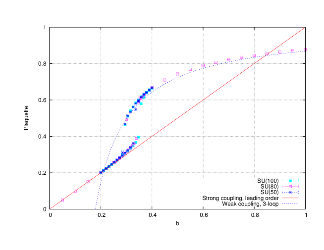
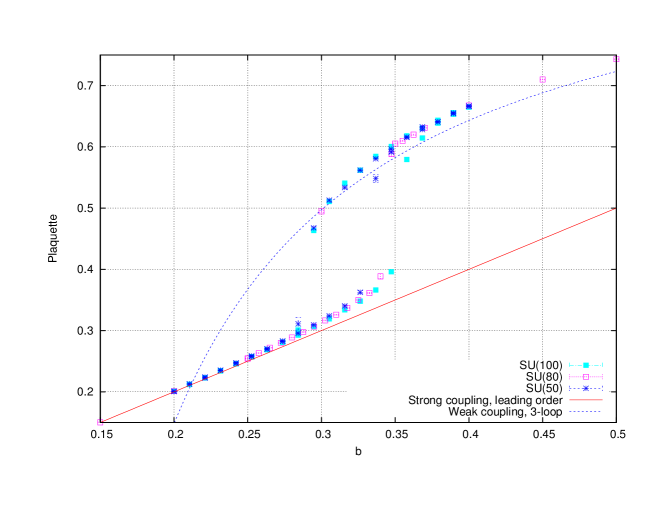
Figure 5: Hysteresis plots of the plaquette variable $u_{p}$ versus $b$ for $SU(50)$ ([blue] crosses), $SU(80)$ ([magenta] open squares), and $SU(100)$ ([light blue] filled squares). Results are for $\rho_{\rm clock}$ and self-averaging. The curves are the predictions for $SU(\infty)$ in the strong-coupling expansion to leading order (solid [red] curve) and of the weak-coupling expansion to three loop order (dashed [blue] curve) (taken from, for example, Ref. TEK ). The lower-panel shows a close-up of the strong-to-weak transition region.

At first glance, the plots appear consistent with the validity of reduction. The results for $u_{p}$ are close to the analytic predictions and to the numerical results from large volume, large-$N$ simulations (although we do not show the latter here). The increasing hysteresis with increasing $N$ is indicative of a strongly first order phase transition somewhere in the range $b_{t}\simeq 0.30-0.35$, which is indeed close to the coupling, $b_{\rm bulk}\simeq 0.36$, at which the well-known “bulk” transition occurs in the large-$N$ gauge theory Mike .

Below, and in the next three sub-sections, we show that this impression is wrong. A clear signal for this can be seen in Fig. (6), which shows how the absolute values $|M_{\mu,\nu}|$ depend on $b$. We recall that the $M_{\mu,\nu}$ transform non-trivially under center and reflection symmetries. The discussion of Sec. IV.2 implies that, for reduction to hold, the $|M_{\mu,\nu}|^{2}$ must have expectation values of $O(1/N)$, and thus that the $\langle|M_{\mu,\nu}|\rangle$ should fall to zero as $N\to\infty$.

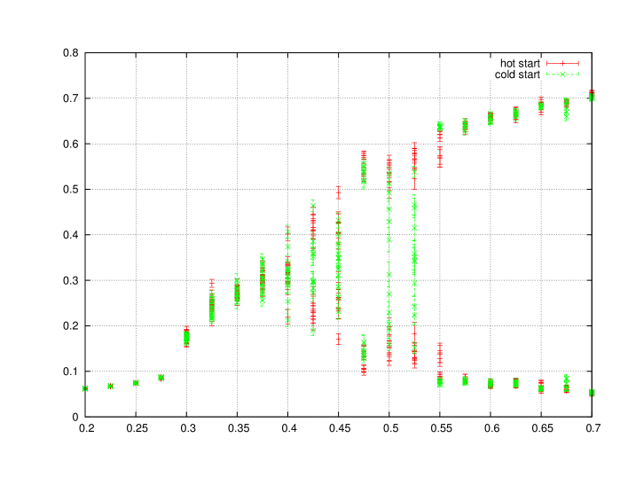
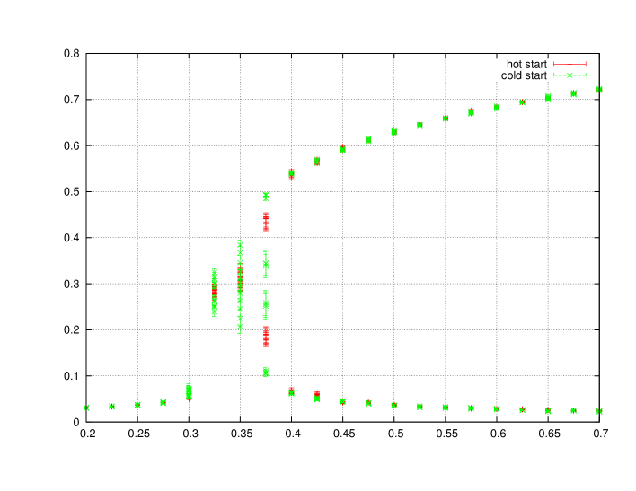
Figure 6: The values of all twelve $\langle|M_{\mu,\nu}|\rangle$ plotted versus $b$ for $N=20$ (upper panel) and $N=40$ (lower panel), using $\rho_{\rm clock}$ and self-averaging.

In fact what we find is that some of the $M_{\mu,\nu}$ fluctuate around $O(1)$ values in the weak-coupling phase. This is the first indication that reduction does not hold in the QEK model.

This result calls for a more detailed study of systematic errors. These include the possibility of very large $O(1/N)$ corrections (i.e. that the non-zero values for $\langle|M_{\mu,\nu}|\rangle$ would decrease for large enough $N$), dependence on the choice $\rho(p)$ or on the self-averaging strategy, and the possibility that the simulations did not, in fact, equilibrate (and that given enough updates would tunnel into a “vacuum” that satisfies reduction). In addition, a more accurate determination of the transition coupling $b_{t}$ would allow a direct test of reduction. This is the coupling at which the QEK model goes through a first order transition, and, if reduction holds, should equal the bulk-transition coupling $b_{\rm bulk}$ of the infinite-volume, large-$N$, pure-gauge theory. In the past, the numerical proximity of $b_{t}$ and $b_{\rm bulk}$ was considered to be evidence in favor of large-$N$ equivalence BHN2 ; Okawa2 ; BM ; Lewis ; Carlson , but the calculations of $b_{t}$ were not of high accuracy. In the next sub-sections we attempt to address all these issues.

V.3 Precise measurements of the plaquette

In this section we perform high-precision measurements of $u_{p}$ for $b=0.4$, $0.45$ and $0.5$, values chosen to allow comparison with results from the large volume simulations of Ref. TV ; Mike . We use and test both strategy A (explicit quenched averaging), and strategy B (self-averaging), and in addition study different choices for the measure $\rho(p)$. To implement strategy A we draw a new choice for $p$ (drawn randomly with weighting $\rho(p)$) after a fixed number of equilibration and measurement sweeps. The simulation parameters are given in Table 2. For strategy B we simply use very long runs with a fixed choice of $p$. Details are given in Table 3.

$N$	choices of $p$	equilibration updates	measurements	$\rho(p)$
$20$, $40$, $80$	$20$	$1000$	$5000$	clock
$40$	20	$5000$	$1000$ and $2000$	uniform

Table 2: Simulation details for measurements of $u_{p}$ using strategy A—explicit quenched averaging. The number of equilibration updates and measurements is for each value of $p$. We use $b=0.4$, $0.45$ and $0.5$ in all cases.

$N$	equilibration updates	measurements	choice of $\rho(p)$ and $p$
$20$, $40$, $80$	$5000$	$100000$	clock ($p=p_{\rm locked}$ or permutation)
$20$, $40$	$5000$	$100000$	uniform
$80$	$1000-5000$	$10000$	uniform
$50$	$1000$	$20000$	clock ($p=p_{\rm locked}$)
$100,125,150,200$	$500$	$1000$	clock ($p=p_{\rm locked}$)
$16$, $81$	$5000$	$100000$	BZ

Table 3: Parameters of simulations used to calculate $u_{p}$ using strategy B—self-averaging. We use $b=0.4$, $0.45$ and $0.5$ except for $N=50$, where we only use $b=0.4$ and $0.5$, and for $N=100$, $125$, $150$, $200$, where we only use $b=0.4$.

We begin by comparing the plaquette time histories for the two strategies. In Fig. 7 we show results for $N=40$ at $b=0.40$ and for $N=80$ at $b=0.50$, in both cases using $\rho_{\rm clock}(p)$.

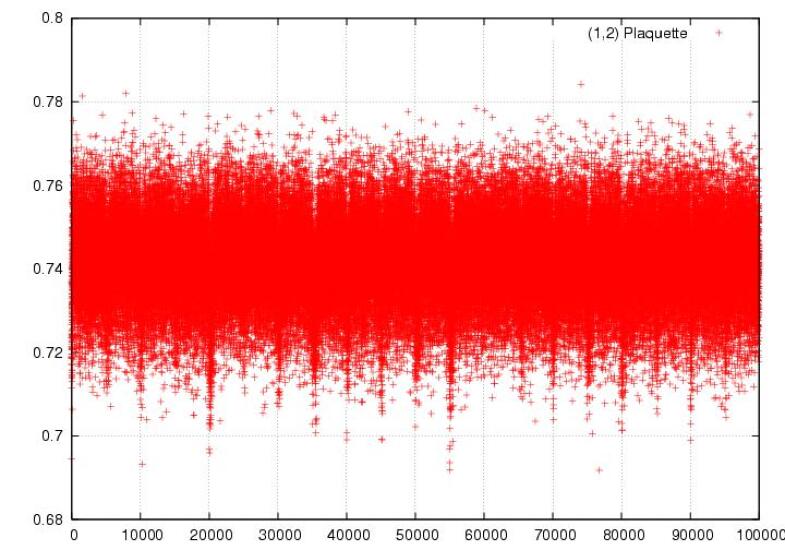
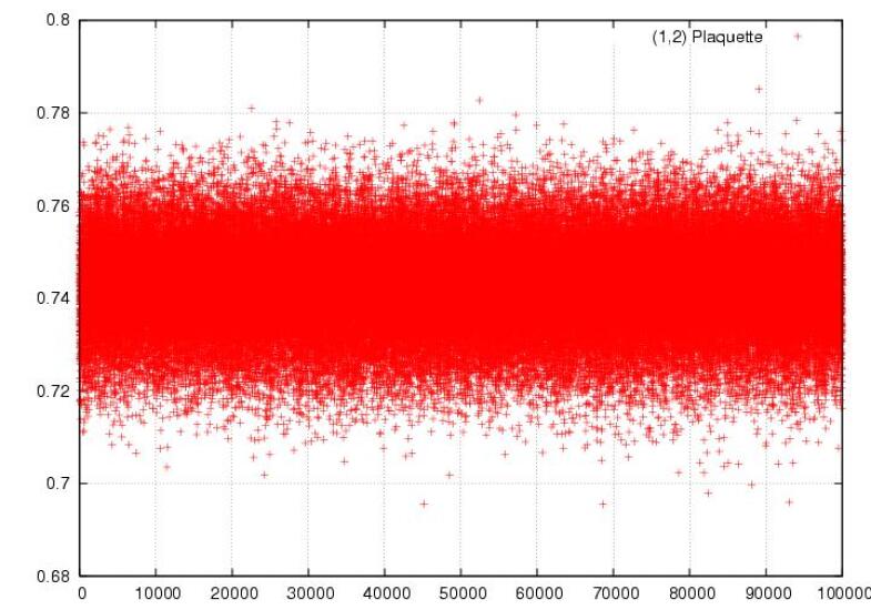
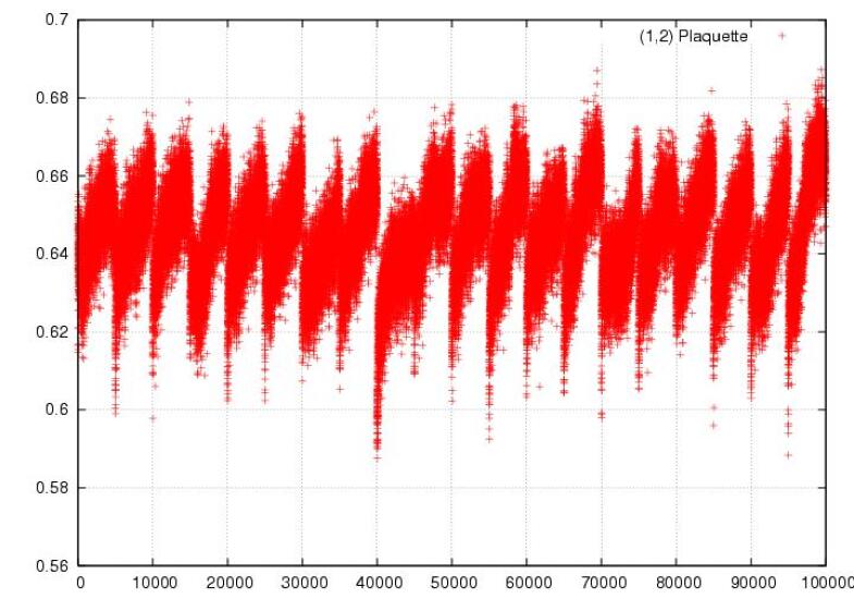
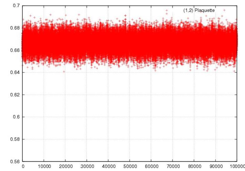
Figure 7: The ($\mu=1$, $\nu=2$) plaquette variable vs measurement number. Equilibration updates are not shown. The upper two panels are for $SU(40)$ with $b=0.5$, the lower two for $SU(80)$ with $b=0.4$. The left-hand plots are for strategy A, in which a random permutation of the clock momenta is generated every 5000 measurements. The right-hand plots are for strategy B, with $p=p_{\rm locked}$.

The results for $N=40$ suggest that, once equilibrated, both strategies give similar results. The “tails” below the main band for strategy A indicate, however, that insufficient equilibration sweeps were included. This effect is much clearer for $N=80$, because of the smaller fluctuations. To see what happens with sufficient equilibration, we present in Fig. 8 the time histories for $SU(40)$ at $b=0.50$, obtained using strategy B, with both $p=p_{\rm locked}$ and a single fixed random permutation. After a long period in a metastable state, with a relatively low value of $u_{p}$, the system does appear to tunnel into a state with a plaquette value consistent with that for $p=p_{\rm locked}$. The time this requires (about 15000 measurements) exceeds, however, that used in our strategy A runs.

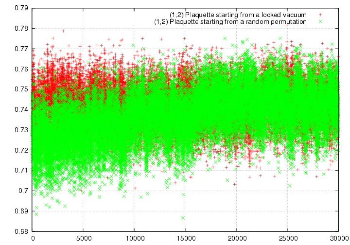
Figure 8: The $(\mu,\nu)=(1,2)$ plaquette variable for $SU(40)$ at $b=0.50$ vs. update with strategy B (self-averaging) with $\rho_{\rm clock}$. [Red] plusses are for $p=p_{\rm locked}$, while [green] crosses are for a random permutation of the clock momenta.

We tentatively conclude that self-averaging works at least approximately for the plaquette, given long enough equilibration times. This conclusion is supported by the results from the other simulations listed in Tables 2 and 3. To illustrate this, we collect, in Tables 4 and 5, the average values of $u_{p}$ using both strategies and for clock and uniform densities. For strategy B we show only results from runs that were equilibrated. For strategy A all results are suspect because of the thermalization issues discussed above and illustrated by Fig. 7. We nevertheless include them as a comparison. The table also includes the best estimates for the plaquette values for $SU(\infty)$, obtained by extrapolating from large-volume simulations Mike-Helvio . These are the numbers that would be reproduced by a large $N$ extrapolation of QEK results were reduction to hold.

We first comment on the results using strategy B. We first note (from Table 4) that, in all cases, the final plaquette is independent of the choice of input momenta for $\rho=\rho_{\rm clock}$. This is the expected self-averaging for a center-invariant quantity. More striking is that, as $N$ increases, results from strategy B using $\rho_{\rm uniform}$ appear to converge to those from $\rho_{\rm clock}$. This gives us confidence that we are not observing systematic errors due to the choice of $\rho$, and that the systematic differences with the results from strategy A are due to lack of equilibration of the latter.

$b$, $u_{p}$ for $SU(\infty)$	Strategy and $\rho(p)$	$SU(20)$	$SU(40)$	$SU(80)$
$b=0.50$, $u_{p}\simeq 0.7182$	A, clock⋆	0.7294(2)	0.7256(2)	0.7223(4)
	B, clock ($p=p_{\rm locked}$)	0.7396(5)	0.7425(2)	0.7429(1)
	B, clock ($p={\rm random}$)	0.739(1)	0.7424(1)	0.7429(1)
	A, uniform⋆	0.7401(3)	–	–
	B, uniform	0.7483(3)	0.7405(2)	0.7432(1)
$b=0.45$, $u_{p}\simeq 0.6795$	A, clock⋆	0.6968(5)	0.7090(1)	0.6867(8)
	B, clock ($p=p_{\rm locked}$)	0.7035(9)	0.7094(1)	0.7100(1)
	B, clock ($p={\rm random}$)	0.703(1)	0.7095(1)	0.7101(1)
	A, uniform⋆	0.7082(4)	–	–
	B, uniform	0.7153(2)	0.7086(2)	0.7100(1)
$b=0.40$, $u_{p}\simeq 0.6259$	A, clock⋆	0.6533(5)	0.6489(7)	0.645(1)
	B, clock ($p=p_{\rm locked}$)	0.66014(54)	0.6651(2)	0.6665(1)
	B, clock ($p={\rm random}$)	0.6595(5)	0.6645(3)	0.6665(1)
	A, uniform⋆	0.6648(5)	–	–
	B, uniform	0.6737(5)	0.6652(2)	0.6642(3)

Table 4: Comparison of plaquette expectation values between averaging strategies and different choices of $\rho(p)$. The results from strategy A are denoted by a “^⋆” to indicate that they are suspect due to a possible lack of equilibration (see text). The first column includes the estimates for $SU(\infty)$ based on extrapolations using large-volume simulations from Ref. Mike-Helvio .

$SU(50)$	$SU(100)$	$SU(125)$	$SU(150)$	$SU(200)$
0.6662(9)	0.6647(3)	0.6658(3)	0.6667(3)	0.6670(2)

Table 5: Additional results for $u_{p}$ obtained with strategy B at $b=0.40$ with $\rho_{\rm clock}$ and $p=p_{\rm locked}$.

The most important comparison is with the results for the infinite-volume $SU(\infty)$ theory. To make this more precise , we extended the results at $b=0.4$ up to $N=200$ (see Table 5). The resulting comparisons are shown in Fig. (9). We have plotted $u_{p}$ versus $1/N$, since this is the expected $N$ dependence in the QEK model. Our results show a fairly smooth extrapolation to $N=\infty$, with small corrections whose dependence on $1/N$ we cannot definitely determine. We do not perform a detailed fit, however, since it is clear that, regardless of the precise form of the subleading terms, our results extrapolate to significantly higher values of $u_{p}$ than those of the infinite-volume lattice gauge theory. This discrepancy clearly shows that the QEK model does not reproduce the physics of the large-$N$ gauge theory.

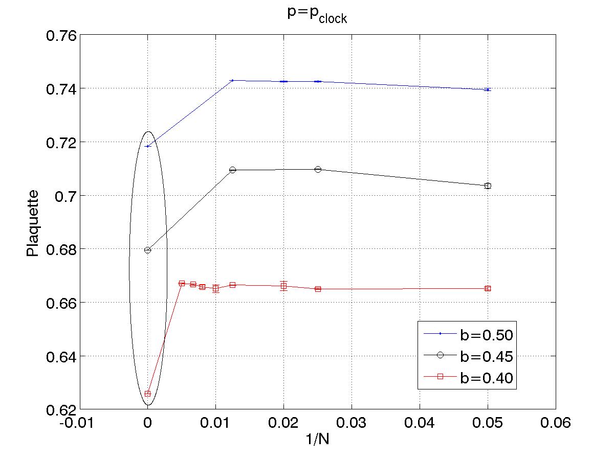
Figure 9: $u_{p}$ versus $1/N$, for $b=0.4$, $0.45$ and $0.5$, compared to the expectations for infinite-volume $SU(\infty)$ gauge theory (presented inside the ellipse). Lines are only to guide the eye. Results shown are for $\rho=\rho_{\rm clock}$ with $p=p_{\rm locked}$.

We have also obtained results using $\rho_{\rm BZ}$. These are collected in Table 6, and the comparison to the lattice large-$N$ result is shown in Fig. 10. The discrepancy with infinite-volume $SU(\infty)$ values is significantly larger in this case, a point we return to below.

$N$	$b=0.4$	$b=0.45$	$b=0.5$
$16$	0.88627(5)	0.89935(4)	0.90961(3)
$81$	0.812323(2)	0.83546(1)	0.85291(1)

Table 6: Results for $u_{p}$ using strategy B for $\rho_{\rm BZ}$.

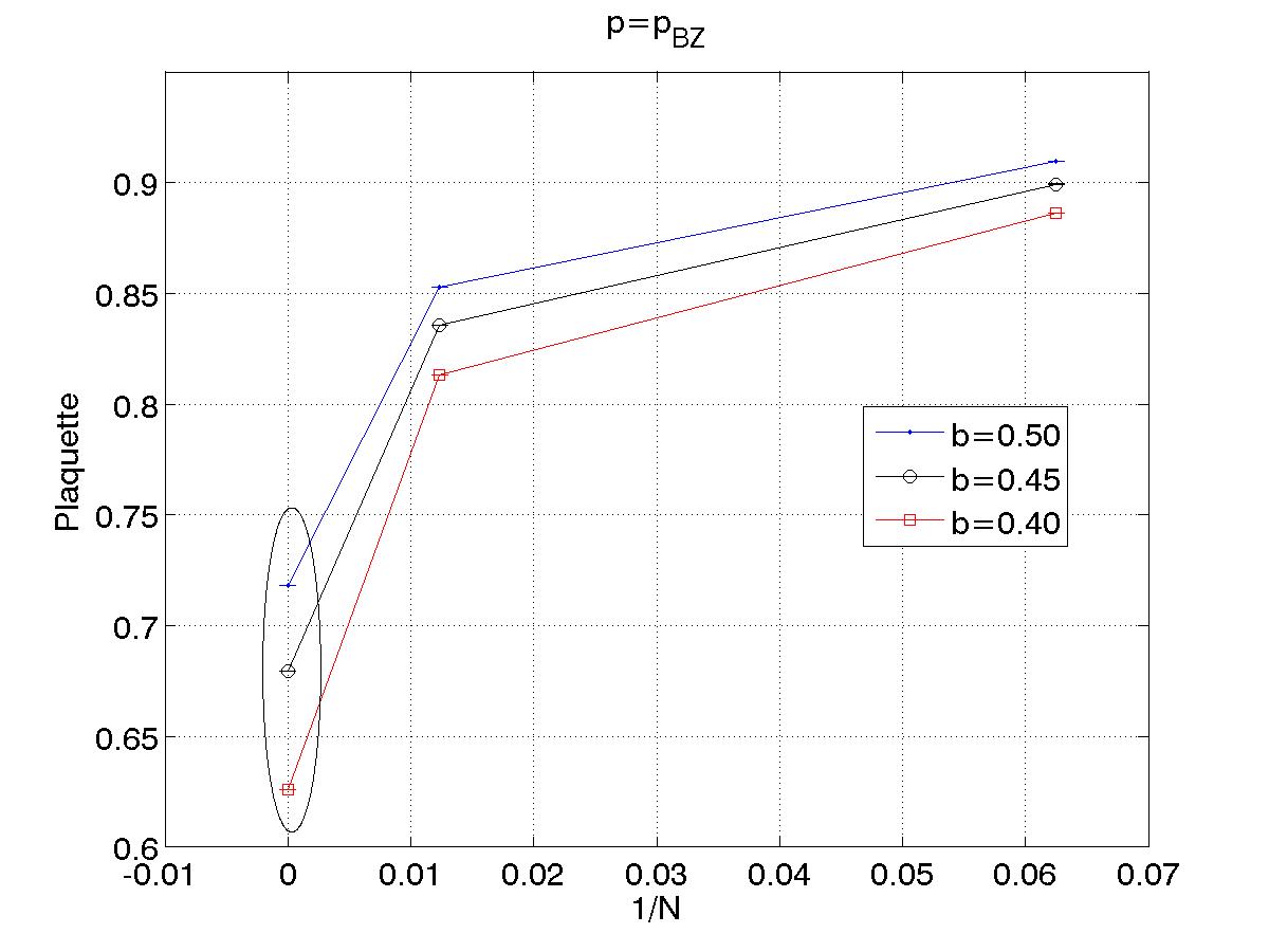
Figure 10: As in Fig. 9, but for $\rho_{\rm BZ}$. Note that the vertical scale differs from Fig.9.

V.4 Precise measurements of the $M_{\mu,\nu}$

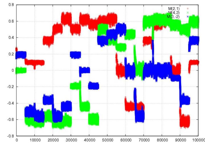
Figure 11: Real part of $M_{\mu,\nu}$ versus measurement number for $N=40$ and $b=0.50$ with $\rho_{\rm clock}(p)$. The figure shows a sequence of $20$ Monte-Carlo runs, each with $1000$ equilibration updates (not shown) followed by $5000$ measurements, and each with a randomly chosen permutation of the clock momenta. For clarity, we only present $M_{2,1}$ ([red] plusses), $M_{4,3}$ ([green] crosses), and $M_{3,-2}$ ([blue] fancy crosses).

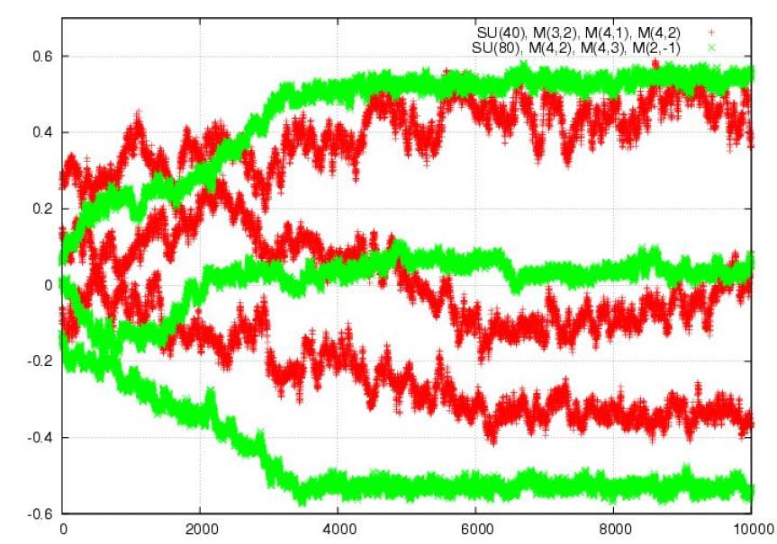
Figure 12: Real part of $M_{\mu,\nu}$ versus measurement number for $\rho_{\rm uniform}(p)$, with a single random $p$, at $b=0.5$ and for $N=40$ ([red] plusses) and $80$ ([green] crosses). We show only $M_{3,2}$, $M_{4,1}$, and $M_{4,2}$ for $SU(40)$, and $M_{4,2}$, $M_{4,3}$, and $M_{2,-1}$ for $SU(80)$.

To elucidate the nature of the breakdown of reduction, we present here results for the “order parameters” $M_{\mu,\nu}$. We use the same simulation parameters as in the previous section. We recall that, for reduction to hold, $\langle|M_{\mu,\nu}|^{2}\rangle_{p}$ should be no larger than $O(1/N)$ for all $\mu$ and $\nu$. Furthermore, for the case of $\rho_{\rm clock}$, the expectation values $\langle M_{\mu\nu}\rangle_{p}$ are true order parameters for spontaneous breakdown of the center symmetry.

We begin by presenting, in Fig. 11, the Monte-Carlo time history of the real parts of a selection of the $M_{\mu,\nu}$, using $\rho(p)=\rho_{\rm clock}(p)$ and strategy A (explicit quenched averaging), for $N=40$ and $b=0.50$. This is the run for which we have previously shown the plaquette in the upper-left panel of Fig. 7. We clearly see equilibration into distinct “vacua” for different choices of input momenta, and in several cases we can see the tail-end of what appears to be a tunneling process. The values of ${\rm Re}(M_{\mu,\nu})$ either oscillate around zero or around values of $O(1)$. The latter indicate SSB of the center symmetry, and the presence of the locked momenta discussed in Sec. IV.1.

We show a similar plot for $\rho_{\rm uniform}(p)$ in Fig. 12, except that we use only a single random choice of $p$, have longer runs to assure equilibration, and present results for both $N=40$ and $80$. After a long equilibration period, the $M_{\mu,\nu}$ at both $N$ fluctuate around what we assume to be vacuum values. We note that the fluctuations are smaller for the larger $N$, as expected in general. We see this behavior throughout our study. The crucial observations, however, are that some of the $M_{\mu,\nu}$ fluctuate around non-zero $O(1)$ values (indicating locked momenta), and that these values are comparable for both $N$. This implies that the left-hand side of Eq. (47) is of $O(1)$, and reduction does not hold.

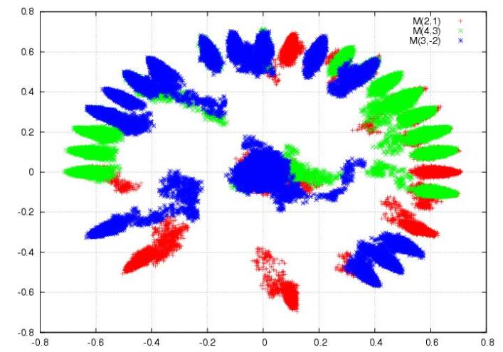
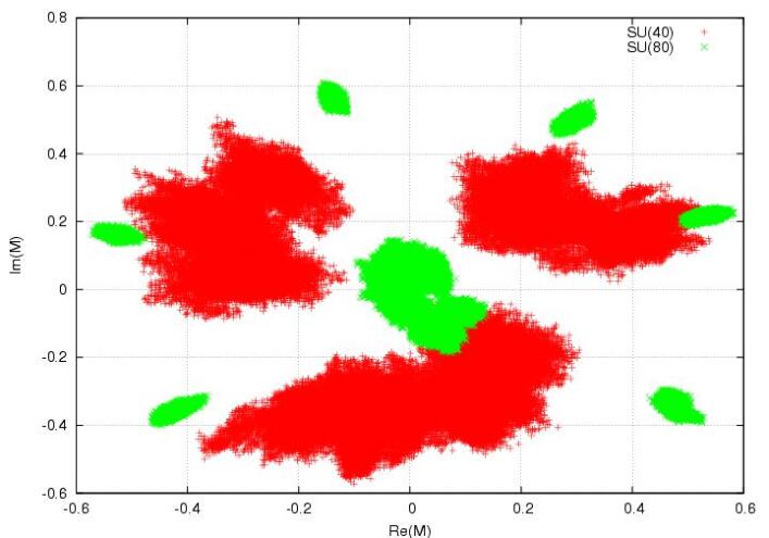
Figure 13: Left panel: scatter plot of the data that appears in the Fig. 11. Right panel: scatter plot of all twelve $M_{\mu,\nu}$ obtained from runs with $\rho(p)=\rho_{\rm uniform}(p)$ for $SU(40)$ ([red] plusses) and $SU(80)$ ([green] crosses) at $b=0.50$, with only equilibrated results shown.

It is also instructive to look at the full complex values of the $M_{\mu,\nu}$. In the left panel of Fig. 13 we show the scatter plot for the same data-set used in Fig. 11. Apart from “equilibration tails”, we see that the simulations settle down into vacua in which a given $M_{\mu,\nu}$ either fluctuates around $0$ or around $m_{0}\exp(2\pi in/40)$, with $n$ an integer and $m_{0}\approx 0.65$. The different vacua are related by (an appropriate subgroup of the $(Z_{N})^{4}$) transformations. This is qualitatively consistent with what we would expect with locked vacua when fluctuations are included. Without fluctuations, the locked vacua have half of the $M_{\mu,\nu}$ vanishing, and the other half of the form $\exp(2\pi in/N)$. The fluctuations reduce the magnitude from unity to $m_{0}$. Note that this reduction is greater than one would predict from a simple mean link model, in which $m_{0}\approx\sqrt{u_{p}}\approx 0.86$. This may be a consequence of the fact that the partial unlocking of momenta can reduce $|M_{\mu\nu}|$ while leaving the plaquette unchanged.

This figure gives a very clear illustration of the way in which $\langle M_{\mu,\nu}\rangle_{\rm QEK}$ vanishes when using $\rho_{\rm clock}(p)$. One is instructed to average over input momenta which are permutations of the clock momenta. For given input momenta, the dynamics picks a (partially) locked vacuum. As the average is taken, each $M_{\mu,\nu}$ will end up with equal probability in the center near the origin, or in the “ring” of radius $m_{0}$, and in the latter case with equal probability in each of the $N$ vacua. In this way $M_{\mu,\nu}$ will average to zero. As noted in Sec. IV, the dynamics will determine whether, for a given input momenta and as $N\to\infty$, the theory gets trapped in a single vacuum or moves between them. Our numerical results strongly indicate the former, in which case (for $\rho_{\rm clock}$) SSB is occurring.

A similar scatter plot for $\rho_{\rm uniform}$ is shown in the right panel of Fig. 13. In this case all twelve $M_{\mu,\nu}$ are shown for each $N$ (not just the three for each $N$ shown in Fig.  12), and we display only measurements after equilibration. For $\rho_{\rm uniform}$ there is no center symmetry, but we do see (most clearly for $N=80$) the expected pattern for locked momenta of six non-zero and six near-zero magnitudes. (Note that some of the [red] $N=40$ points near the origin are obscured by the [green] $N=80$ points.) We also observe no reduction in the $O(1)$ magnitudes as $N$ increases from $40$ to $80$—indeed the magnitudes seem to increase. This we take as strong evidence for the breakdown of reduction.

Finally, we consider $\rho_{\rm BZ}$. We show results obtained only from a hot start. In the left panel of Fig. 14, we show the time history of all the $M_{\mu,\nu}$ for $N=16$ and $b=0.40$. Recalling the definition of $\rho_{\rm BZ}$ from Eq. (38), we note that, since $K=\sqrt[4]{16}=2$, all $p^{a}_{\mu}$ are either $0$ or $\pi$. This means that the $M_{\mu,\nu}$ are real, and that $M_{\mu,\nu}=M_{\mu,-\nu}$ (so there are only 6 independent $M_{\mu,\nu}$). Furthermore, the center symmetry is only $(Z_{2})^{4}$, although this symmetry group is still sufficient to forbid expectation values for the $M_{\mu,\nu}$. What we see from the figure is that while four of the $M_{\mu,\nu}$ fluctuate around zero, two of them ($M_{1,2}$ and $M_{4,2}$ ) acquire nonzero expectation values that break the $(Z_{2})^{4}$ symmetry.

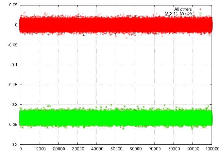
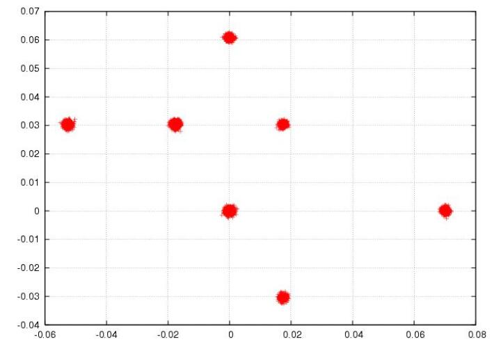
Figure 14: Results for $M_{\mu,\nu}$ with $\rho_{\rm BZ}$. Left panel: Time history (versus measurement number) of all six independent $M_{\mu,\nu}$ for $N=16$ and $b=0.40$. Right panel: Scatter plot of all $M_{\mu,\nu}$ for $N=81$ and $b=0.70$.

We can understand this pattern of expectation values in the following way. The input momenta [defined in Eq. (38)] are such that

$$\Lambda_{1} = {\rm diag}(\sigma_{3},\sigma_{3},\dots)\,,\ \ \Lambda_{2}={\rm diag}(\bm{1}_{2},-\bm{1}_{2},\bm{1}_{2},-\bm{1}_{2},\dots)\,,\ \$$

$$\Lambda_{3} = {\rm diag}(\bm{1}_{4},-\bm{1}_{4},\bm{1}_{4},-\bm{1}_{4})\,,\ \ \Lambda_{4}={\rm diag}(\bm{1}_{8},-\bm{1}_{8})\,,$$ (61)

where $\bm{1}_{n}$ indicates (the diagonal part of) an $n$-dimensional identity matrix. With these matrices, and assuming $U_{\mu}\approx\Lambda_{\mu}$ (i.e. ignoring fluctuations due to the $V_{\mu}$), all the $M_{\mu,\nu}$ vanish. By a single transposition, however, one can change $\Lambda_{2}$ to

$$\Lambda^{\prime}_{2}={\rm diag}(-\sigma_{3},-\bm{1}_{2},\bm{1}_{2},-\bm{1}_{2},\bm{1}_{2},-\sigma_{3},\bm{1}_{2},-\bm{1}_{2})\,.$$ (62)

One then finds, in the same approximation of ignoring fluctuations, that there are two non-zero $M_{\mu,\nu}$: $M_{1,2}=M_{2,4}=-0.25$. Fluctuations will reduce the average from this value. Thus this scenario provides a possible explanation for the results of the left panel of Fig. 14. This is, in fact, one of many choices of transpositions that leads to this pattern of expectation values. Furthermore, all the patterns of values for the $M_{\mu,\nu}$ that we have observed in our $N=16$ runs can be explained similarly.

We see an analogous phenomenon for $N=81$. Here, since $K=3$, the center symmetry is $(Z_{3})^{4}$. The right panel of Fig. 14 shows a scatter plot of all the (now twelve) $M_{\mu,\nu}$ from a simulation at $b=0.70$. One can understand this figure by calculating the possible values of $M_{\mu,\nu}$ that are obtained by permuting the elements of the initial $\Lambda_{\mu}$, and ignoring fluctuations. The result is shown in Fig. 15, and is clearly a good description of what we see in the right panel of Fig. 14.

Figure 15: Some of the possible values for $M_{\mu,\nu}$ in the $N=81$ case, assuming no fluctuations, i.e. when the $p_{\mu}^{a}$ are permutations of $p_{BZ}$. Note that, in a given simulation, one expects only some (at most 12) of these values to be realized. This figure should be compared to the right panel of Fig. 14.

We note that, unlike for $\rho_{\rm clock}$, the BZ weight function does not lead to complete or nearly-complete momentum locking. In a completely locked state, all the $\Lambda_{\mu}$ are equal up to center and reflection transformations, and this leads, in the example of $N=2$, to all six independent $M_{\mu,\nu}$ being close to $\pm 1$. To reach such a locked state requires many transpositions, however, and our results suggest that only a few transpositions have occurred.

In summary, the numerical results presented in this sub-section indicate that some of the “order parameters” $M_{\mu\nu}$ acquire $O(1)$ expectation values, which, as described in Sec. IV, is inconsistent with large-$N$ reduction for the QEK model. For the weight functions $\rho_{\rm clock}$ and $\rho_{\rm BZ}$, the expectation values for the $M_{\mu,\nu}$ spontaneously break the center and reflection symmetries. This breakdown is not apparent in the simplest open loops, i.e. $\langle{\text{t}r}\,U_{\mu}^{n}\rangle$ with $n<N$, but is exhibited by more complicated objects like the “corner” variables $M_{\mu,\nu}$. For the uniform and clock distributions, the actual values of the $M_{\mu,\nu}$ are qualitatively consistent with the “momentum-locking” predicted by the weak-coupling analysis. That analysis, however, could not determine whether the symmetry-breaking or cluster-decomposition-violating scenario would hold. Our numerical results clearly favor the former.

V.5 Precise measurements of the transition coupling $b_{t}$

The plaquette data in Fig. (5) strongly suggest that the QEK model has a first order phase transition for $b$ somewhere in the range $0.30-0.33$. This was already noted in the early QEK literature BHN2 ; Okawa2 ; Bhanot ; BM , and the transition was assumed to be the same as that which occurs in the $SU(\infty)$ gauge theory at $b_{\rm Bulk}\simeq 0.36$ (the “bulk transition”). The $\sim 10\%$ discrepancy was attributed to $O(1/N)$ corrections and/or other systematic errors. In this section we revisit this issue, and, in particular, attempt to greatly reduce the systematic errors in the determination of $b_{t}$.

The main source of uncertainty is the strongly first-order nature of the transition, and the consequent metastability. The strength of the transition is indicated by the size of the jump in the plaquette, which is $\sim 0.3$. Although, strictly speaking, there is no transition unless $N\to\infty$, already for $N=50$ there is a significant hysteresis regime of width $\Delta b\simeq 0.05$, and this width increases with $N$. Thus an estimate of $b_{t}$ from Fig. 5 has an $O(15\%)$ error at $N=50$, and this error too increases with $N$. It does not help to calculate $u_{p}$ on a denser grid, because of the metastability.

One way forward is to use re-weighting, making use of those values of $b$ where tunneling between phases occurs. We expect the tunneling probability to fall exponentially with $N^{2}$ (which counts the number of degrees of freedom and thus is like the volume), and our results are qualitatively consistent with this. We find that we can successfully use standard Ferrenberg-Swendsen (FS) re-weighting FS for $N=20$ and $30$, but for $N$ larger than about $40$ the method fails because tunneling ceases.

To proceed we need a method which encourages tunneling. We chose to use the “Wang-Landau” re-weighting method, developed recently in the field of statistical mechanics WL . This required adapting the method from spin-systems to gauge theories, as well as developing a systematic way of estimating errors. Presenting this analysis is beyond the scope of this paper, and is presented in Ref. WL_paper . We note only that this is an adaptive method of determining the density of states, which includes a feature that forces motion through configuration space.

Type of re-weighting	$\ SU(20)$	$\ SU(30)$	$\ SU(40)$	$\ SU(50)$
Ferrenberg-Swendsen	0.29598(5)	0.30545(5)	–	–
Wang-Landau	0.29544(37)	0.30569(17)	0.30968(20)	0.31121(19)

Table 7: Values of the strong-weak transition coupling $b_{t}$, obtained for $\rho_{\rm clock}(p)$ with $p=p_{\rm locked}$, with two different re-weighting methods.

We have carried out these calculations only for $\rho=\rho_{\rm clock}$ and with input momenta being locked. Since the algorithms are designed to ensure ergodicity, however, we expect that the simulations will explore multiple permutations of the momenta, i.e. will be self-averaging. Evidence in support of this expectation is that we do see many tunnelings between the weak and strong phases for all $N$. Table 7 gives our results for the transition coupling (defined as the peak in the susceptibility). We find that the results from both techniques agree (when both are available) despite the very small ($0.02\%-0.1\%$) statistical errors.

We plot these results versus $1/N$ in Fig. (16). For comparison, we include estimates of $b_{t}$ from the old numerical studies in Refs. BHN2 ; Okawa2 ; Bhanot ; BM , as well as the most recent estimates of the coupling $b_{\rm bulk}$ at which the bulk transition occurs in the infinite volume $SU(\infty)$ gauge theory Mike . While our new results are consistent with the old numerical studies of the QEK model, it is very unlikely that they extrapolate to the vicinity of $b_{\rm bulk}$. We stress, however, that to make this observation, it is crucial to have very small errors, and this was accomplished with the Wang-Landau algorithm.

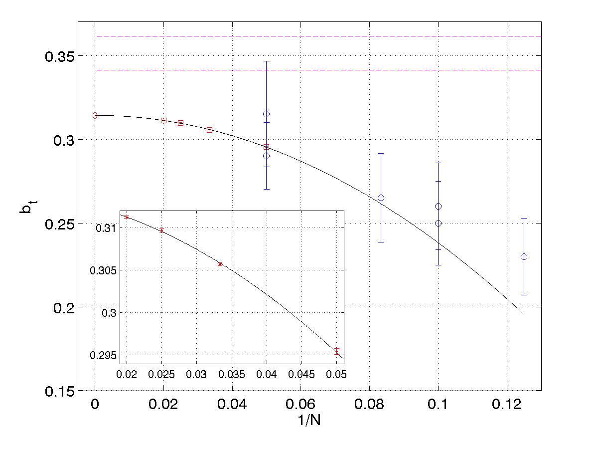
Figure 16: The strong-to-weak transition coupling, $b_{t}$, plotted versus $1/N$. [Red] squares show our results using the Wang-Landau algorithm from Table 7, while [blue] circles are from Refs. BHN2 ; Okawa2 ; Bhanot ; BM . The solid black curve is the fit described in the text. The [magenta] dashed horizontal lines give the range in which the bulk transition in $SU(12)$ should take place, according to hysteresis scans performed in a lattice theory Mike . The insert shows a close-up of our new data.

We fit the Wang-Landau data (i.e. the second row in Table 7) to the form

$$b_{t}(N)=b_{t}(\infty)+\frac{A}{N}+\frac{B}{N^{2}}\,,$$ (63)

and find the fit parameters listed in Table 8. The fits are of reasonable quality, and find values for $b_{t}(\infty)$ which lie well below the estimate $b_{\rm bulk}\simeq 0.36$. It is hard to quote a significance for this discrepancy, since we do not have a good estimate of the error in $b_{\rm bulk}$. If we use the error in our results, the significance is between $\sim 50$ to $\sim 200$ $\sigma$. We thus think it is very unlikely that $b_{t}$ in the QEK model can be identified with $b_{\rm bulk}$ of the $SU(\infty)$ lattice gauge theory.

We have compared fits with and without the $1/N$ term, and find that the former is slightly preferred, as shown in the Table. It is this fit which is included in Fig. (16). We have also attempted to fit simultaneously to the Wang-Landau results for $N=40$ and $50$ and the (more accurate) FS results for $N=20$ and $30$. This fit fails, quite likely because, given the very high accuracy obtained with the FS method, we need to include terms of $O(1/N^{3})$.

Type of fit	$b_{t}(\infty)$	$A$	$B$	$\chi^{2}/{\rm d.o.f.}$
$A=0,B\neq 0$	0.3142(2)	–	-7.59(18)	$1.45/1$
$A\neq 0,B\neq 0$	0.3148(10)	-0.037(65)	-7.06(97)	1.1/1

Table 8: The parameters $b_{t}(\infty)$, $A$, and $B$, obtained from fitting the Wang-Landau data in Table 7 to the form Eq. (63).

VI Summary and discussion

In this paper we have studied the validity of large-$N$ reduction for the four dimensional quenched Eguchi-Kawai model. This model is a variant of the original Eguchi-Kawai model in which the distribution of the eigenvalues of the link matrices is forced to be uniform by quenching, while all other degrees of freedom remain dynamical.

We find that while enforcing a uniform eigenvalue distribution is indeed a necessary condition for large-$N$ reduction to hold, it is not sufficient. The reason is that quenching fixes the eigenvalues only up to permutations that can be performed independently in the four directions. These permutations occur dynamically in the model due to fluctuations in the unquenched degrees of freedom, and can lead to correlations between the ordering of the eigenvalues of the four link matrices. If such correlations occur then we show that the arguments of Refs. BHN1 ; Migdal ; HN ; GK ; Parisi-papers ; DW for the validity of the large-$N$ quenched reduction break down.

The question then is whether such correlations between link eigenvalues occur. We show that they are indeed expected in the weak-coupling regime by minimizing the free energy with respect to the ordering of the eigenvalues. This then leads us to perform a detailed numerical study of the QEK model with intermediate and strong couplings using Monte-Carlo techniques. We find the weak-coupling calculation is indeed a good guide and obtain the following evidence for the breakdown of large-$N$ reduction in the model:

• We observe clear evidence for eigenvalue correlations by measuring order parameters that explicitly probe the correlation between the different link matrices along the different Euclidean directions.

• When we compare the plaquette expectation values of the QEK model and of large volume lattice gauge theories, we find very large discrepancies that do not go away with increasing $N$.

• When we measure the coupling at which a strong-to-weak transition occurs in the QEK model, and compare it to the coupling at which the “bulk” transition takes place in large-$N$ lattice gauge theories in large volumes, we observe a large discrepancy which is of order 13%, and very significant statistically.

We checked that these conclusions are insensitive to the precise form of the quenched eigenvalue distribution, and to the way we perform the quenched average. We also considered values of $N$ up to $200$ to look for a late onset of $1/N$ behavior, but find none. We conclude that the momentum quenched large-$N$ reduction of $SU(N)$ lattice gauge theories fails in the continuum limit.

We have focused in this paper on the behavior in the weak coupling region, since this is where a continuum limit might be taken. Nevertheless, it is also interesting to consider the status of reduction in the strong coupling regime. In the strong-coupling expansion no eigenvalue correlations appear and so the QEK model is expected to be equivalent to the $SU(\infty)$ gauge theory for large enough ‘t Hooft coupling $\lambda$. It follows that reduction is valid until a transition occurs into a phase in which eigenvalue correlations appear. For the quenched Eguchi-Kawai this occurs at the strong-to-weak transition. We have checked numerically that the eigenvalue correlations do vanish on the strong-coupling side of this transition. A similar picture holds for both the EK and TEK models: reduction holds for large enough $\lambda$ but is lost below a certain coupling. We stress, however, that this transition coupling differs for all three theories (and also differs from the bulk transition coupling for $SU(\infty)$). This is just a reflection of the fact that the weak-coupling phases in these theories are unrelated.

These results, together with those of Refs. TV ; Ishikawa concerning the TEK model, mean that, currently, only two single-site models are known that can possibly reproduce the properties of QCD at large-$N$. The first is the “deformed” Eguchi-Kawai (DEK) model, which is the single-site example of a class of models proposed very recently in Ref. DEK . In the DEK, the action of the Eguchi-Kawai model is deformed so that breakdown of the $Z_{N}^{4}$ symmetry is energetically disfavored, and yet at the same time the large-$N$ dynamics is not modified. Thus in this model the original Eguchi-Kawai proof of reduction is expected to remain valid. In preliminary calculations of the DEK model we see that this deformation must include terms that decorrelate the gauge fields in different Euclidean directions, and this makes a direct connection to our results in the QEK model, where we see that such correlation is dynamically preferred. Deformation comes, however, at a cost. Adding all possible deformations is likely to be prohibitively expensive, because there are $\sim N^{4}$ in four dimensions. Whether one can improve this scaling by wise choices of the deformations is a subject for future investigation.

The other single-site candidate is the model obtained by adding $1\leq N_{f}\leq 4$ Majorana adjoint quarks, with periodic boundary conditions, to the Eguchi-Kawai action QCDadjoint . Here the one-loop potential for the link eigenvalues is repulsive if the quark mass in units of the lattice spacing, $a_{\rm lat}m$, is small enough, and reduction is expected to hold. By taking $a_{\rm lat}m\ll 1$ and yet $m$ much larger than the confinement scale $\Lambda$, this single site model should reproduce the pure Yang-Mills theory in the IR, and it remains to be seen how such a construction compares computationally to that of DEK . For $m\ll\Lambda$ this model describes the large-$N$ limit of QCD with adjoint quarks which, for $N_{f}\leq 4$, is expected to confine and to be related to $3$-color QCD through the orientifold large-$N$ equivalence. For $N_{f}\simeq 5$ this model is expected to be close to conformal, and also of interest. We leave the exploration of both these single-site models to future studies.

- (1) G. ’t Hooft, Nucl. Phys. B 75, 461 (1974).
- (2) E. Witten, Nucl. Phys. B 160, 57 (1979).
- (3) For a recent review see K. Peeters and M. Zamaklar, arXiv:0708.1502 [hep-ph].
- (4) M. Teper, [arXiv:hep-lat/0509019].
- (5) R. Narayanan and H. Neuberger, arXiv:0710.0098 [hep-lat].
- (6) T. Eguchi and H. Kawai, Phys. Rev. Lett. 48, 1063 (1982).
- (7) G. Bhanot, U. M. Heller and H. Neuberger, Phys. Lett. B 113, 47 (1982).
- (8) V. A. Kazakov and A. A. Migdal, Phys. Lett. B 116, 423 (1982).
- (9) M. Okawa, Rev. Lett. 49, 353 (1982).
- (10) A. A. Migdal, Phys. Lett. B 116, 425 (1982).
- (11) G. Bhanot, U. M. Heller and H. Neuberger, Phys. Lett. B 115, 237 (1982).
- (12) M. Okawa, Phys. Rev. Lett. 49, 705 (1982).
- (13) G. Bhanot, Presented at Workshop on Nonperturbative Field Theory and QCD, Trieste, Italy, Dec 17-21, 1982. Published in Trieste Field Theor.Wkshp.1982:150
- (14) G. Bhanot and K. J. M. Moriarty, Phys. Lett. B 122, 271 (1983).
- (15) M. R. Lewis, J. Phys. G 11, 981 (1985).
- (16) J. W. Carlson, Phys. Lett. B 127, 115 (1983).
- (17) U. M. Heller and H. Neuberger, Nucl. Phys. B 207, 399 (1982).
- (18) D. J. Gross and Y. Kitazawa, Nucl. Phys. B 206, 440 (1982).
- (19) G. Parisi, Phys. Lett. B 112, 463 (1982). G. Parisi and Y. C. Zhang, Nucl. Phys. B 216, 408 (1983). G. Parisi and Y. C. Zhang, Lett. B 114 (1982) 319.
- (20) S. R. Das and S. R. Wadia, Phys. Lett. B 117, 228 (1982).
- (21) H. Neuberger, Phys. Lett. B 119, 179 (1982), Nucl. Phys. B 220, 237 (1983).
- (22) N. H. Parsons, J. Phys. G 10, 1319 (1984).
- (23) S. R. Das, Rev. Mod. Phys. 59, 235 (1987).
- (24) Yu. Makeenko, “Methods of contemporary gauge theory,”Cambridge Univ. Press (2002) 417p
- (25) A. A. Migdal, Phys. Rept. 102 (1983) 199.
- (26) A. Gonzalez-Arroyo and M. Okawa, Phys. Lett. B 120, 174 (1983).
- (27) M. Teper and H. Vairinhos, Phys. Lett. B 652, 359 (2007) [arXiv:hep-th/0612097].
- (28) T. Azeyanagi, M. Hanada, T. Hirata and T. Ishikawa, JHEP 0801, 025 (2008) [arXiv:0711.1925 [hep-lat]].
- (29) W. Bietenholz, A. Bigarini, J. Nishimura, Y. Susaki, A. Torrielli and J. Volkholz, arXiv:0708.1857 [hep-lat].
- (30) J. Kiskis, R. Narayanan and H. Neuberger, Phys. Rev. D 66, 025019 (2002) [arXiv:hep-lat/0203005].
- (31) P. Kovtun, M. Unsal and L. G. Yaffe, JHEP 0706, 019 (2007) [arXiv:hep-th/0702021].
- (32) A. Armoni, M. Shifman and G. Veneziano, Nucl. Phys. B 667, 170 (2003) [arXiv:hep-th/0302163].
- (33) M. Unsal and L. G. Yaffe, arXiv:0803.0344 [hep-th].
- (34) A. Coste, A. Gonzalez-Arroyo, J. Jurkiewicz and C. P. Korthals Altes, Nucl. Phys. B 262 (1985) 67.
- (35) I. Bars, Based on lectures given at 21st Int. Conf. on High Energy Physics, Paris, France, Jul 26-31, 1982. Published in Trieste Field Theor.Wkshp.1982:168 unpublished (1983).
- (36) N. D. Mermin and H. Wagner Phys. Rev. Lett. 17, 1133 (1966). S. R. Coleman, Commun. Math. Phys. 31 (1973) 259.
- (37) F. Wang, D. P. Landau, Phys. Rev. Lett. 86, 2050 (2001).
- (38) K. Fabricius and O. Haan, Phys. Lett. 143B, 459 (1984).
- (39) J. Kiskis, R. Narayanan and H. Neuberger, Phys. Lett. B 574, 65 (2003) [arXiv:hep-lat/0308033]. P. de Forcrand and O. Jahn, arXiv:hep-lat/0503041.
- (40) B. Bringoltz and S. R. Sharpe, arXiv:0807.1275 [hep-lat].
- (41) M. Teper, private communications, (2008).
- (42) M. Campostrini, Nucl. Phys. Proc. Suppl. 73, 724 (1999) [arXiv:hep-lat/9809072].
- (43) M. Teper and H. Vairinhos, private communications, (2008).
- (44) A. M. Ferrenberg and R. H. Swendsen, Phys. Rev. Lett. 23, 2635 (1988).