Features and nongaussianity
in the inflationary power spectrum

I summarize recent work on (1) constraining spike-like features in the cosmic microwave background (CMB) and large scale structure (LSS); (2) nonstandard Friedmann equation in stabilized warped 6D brane cosmology, with applications to inflation; and (3) nonlocal inflation models, motivated by string theory, which can yield large nongaussian CMB fluctuations. Work in collaboration with N. Barnaby, T. Biswas, F. Chen, L. Hoi, G. Holder and S. Kanno.

1 Features in the CMB and LSS

It is hoped that with improvements in the CMB and LSS data, fingerprints of the underlying inflationary model may be discovered, in the form of features going beyond the amplitude and tilt of the spectrum. One such feature is the appearance of bumps in the spectrum, which can be caused for example by a tachyonic instability during inflation.$\!{}^{{\bf?}}$ In ref. [2] we undertook a systematic search for evidence of such bumps using the latest CMB and LSS data in conjunction with a modified CosmoMC code. Our initial ansatz for the shape of the bump was motivated by a number of models $\!{}^{{\bf?},{\bf?},{\bf?}}$ and theoretical arguments $\!{}^{{\bf?}}$ for a scale noninvariant addition to the spectrum of the form $\delta P=Ak^{3}$ (thus having spectral index $n_{\sigma}=4$), cut off at some maximum wave number $k_{c}$. This is a model with two extra parameters, $A$ and $k_{c}$, similar to the running spectral index extension of the standard $\Lambda$CDM model, since the latter also introduces the tensor ratio $r$. As we will discuss, the results are rather insensitive to the value $n_{\sigma}=4$, so it makes sense to fix this exponent based on theoretical expectations and keep only two extra parameters.

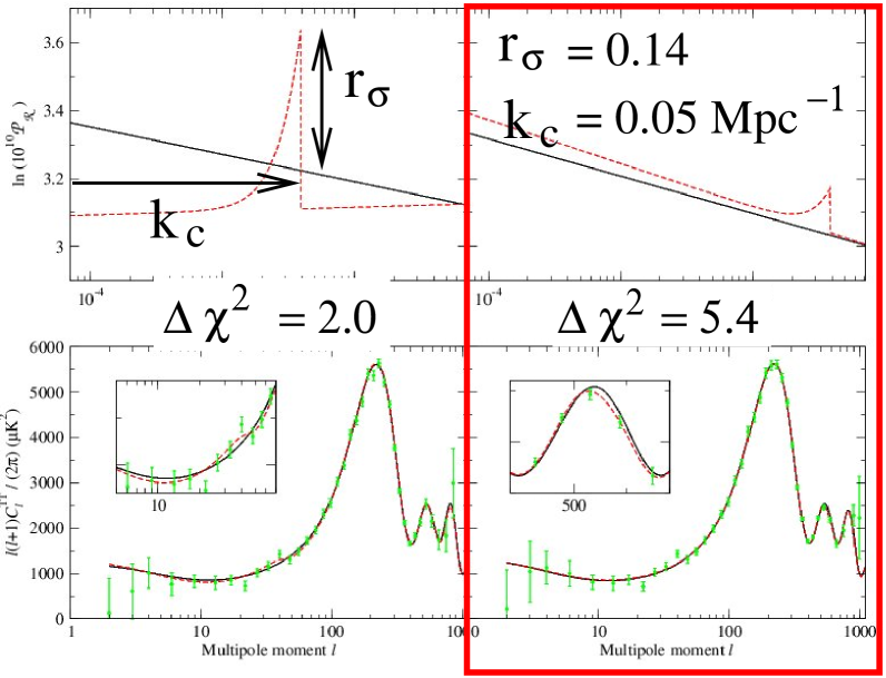
Figure 1: Top panels: standard $\Lambda$CDM power spectrum (solid lines) and best-fit spectrum perturbed by spike (dashed line). Bottom panels: corresponding temperature (TT) multipoles, showing improvements in fit to data.

In figure 1 the top panels show two examples of best-fit cut-off $k^{3}$ spikes found by CosmoMC, superimposed on the best fit $\Lambda$CDM spectrum. We trade the absolute amplitude $A$ of the spike for the parameter $r_{\sigma}$ which denotes its ratio to the amplitude of the standard, nearly-scale-invariant component. The bottom panels show how these spikes in the primordial spectrum, combined with the adjustments of the other cosmological parameters, improve the fit of the model to the WMAP3 data in the two regions, where the standard $\Lambda$CDM prediction (solid curves) either fell above or below the data. The improvement to the fit is most significant for the second spike, in the vicinity of multipole $\ell=550$, giving a reduction in $\chi^{2}$ of 5.4, notably more significant than the improvement which was obtained by the much-discussed running spectral index model. The combination of the spike with a smaller value of $n_{s}$ for the scale invariant component allows for the prediction to be lowered in the vicinity of the feature, and thereby to better match the data, relative to the $\Lambda$CDM prediction. It is striking that such large spikes, and accompanying large changes in $n_{s}$ for the scale invariant component, are not only allowed by the data, but even preferred by it.

Since finishing ref. [2], the WMAP5 data have been released and we have rerun the code with the new data. Interestingly, just like the evidence for the running spectral index, the evidence for the spikes disappears using WMAP5. Instead, we get upper bounds on the amplitude ratio $r_{\sigma}$ as a function of the cutoff $k_{c}$. These will be published in an updated version of ref.  [2].

One may question the assumption of the spectral index $n_{\sigma}=4$ for the nonscale-invariant perturbation. Different values would give rise to a broader or narrower spike. However, these differences in the primordial spectrum tend to get washed out in the multipoles, which involve a convolution of the primordial power. Table 1 gives the change in $\chi^{2}$ for the two features shown in figure 1 when $n_{\sigma}$ varies between 1 and 5; the variation in the improvement to the fits is largely insignificant.

$k^{n}$	$\Delta\chi^{2},\ \ell\sim 50$	$\Delta\chi^{2},\ \ell\sim 540$
$k^{1}$	-0.1	4.1
$k^{2}$	1.2	4.1
$k^{3}$	2.0	5.4
$k^{4}$	1.5	4.8
$k^{5}$	1.9	5.4

Table 1: Comparison of fits using different spectal index for the nonscale-invariant perturbation.

2 Modified Friedmann equation and inflation from a 6D braneworld model

In ref. [6] we have studied the closest generalization of the Randall-Sundrum I model $\!{}^{{\bf?}}$ from 5 to 6 dimensions. The geometry is pictured in fig. 2: it is a warped (nearly AdS) throat with a conical singularity (3-brane) at the bottom, and cut off by a 4-brane at the top, with $Z_{2}$ orbifold boundary conditions. The cosmology of this model was studied earlier in ref. [9], which claimed that the standard Friedmann equation was not recovered even when the extra dimensions were stabilized using a bulk scalar field. In ref. [6] we have corrected this claim, demonstrating that general relativity (GR) is indeed the valid description at low energies.

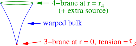
Figure 2: A 6D version of the Randall-Sundrum model, the AdS soliton geometry.

However there are interesting deviations to the Friedmann equations at high scales, illustrated in fig. 3. For given values of the 4-brane tension and bulk cosmological constant, one can find a value of the 3-brane tension for which the 4D vacuum energy vanishes and the solution is static. We model the energy density of the visible universe as excess tension $\delta\tau_{3}$ which gives rise to expansion. The Hubble rate is double valued as a function of $\delta\tau_{3}$, and the two branches smoothly join each other (the “critical point” in fig. 3) at some maximum value of the tension, $\delta\tau_{c}$. The existence of two possible solutions for the same sources of stress-energy also occurs in the DGP model,$\!{}^{{\bf?}}$ where the self-accelerating branch is known to be afflicted with a ghost. In our case, the analysis of small fluctuations reveals that the sickness of the exotic branch is associated with a tachyonic instability of the radion, i.e., the size of the extra dimensions. Under small perturbations, the solutions associated with the exotic branch decompactify. Therefore we disregard the high-$H$ branch in the following.

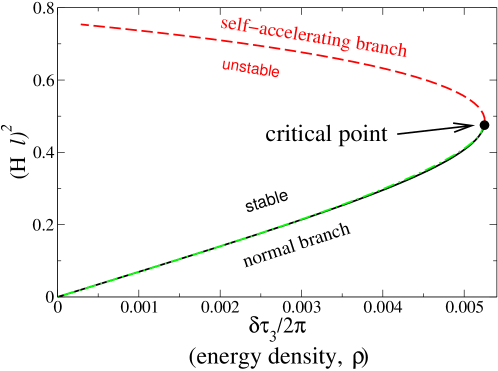
Figure 3: Hubble rate (squared) versus excess brane tension in 6D model.

Nevertheless, interesting departures from GR occur near the critical energy density, $\rho_{c}$. They can be parametrized through a function of the energy density on the 3-brane, ${\cal F}(\rho)=1+O(\rho/\rho_{c})^{2}$, by writing the Friedmann equation in the form $H^{2}={\rho\over 3M_{p}^{2}}{\cal F}(\rho)$. From fig. 3 one notices that the derivative ${\cal F}\,^{\prime}(\rho_{c})$ diverges at the critical point, even though ${\cal F}(\rho_{c})$ is finite. If inflation takes place on the 3-brane, starting with $\rho$ close to $\rho_{c}$, this can give rise to significant changes in the predictions for the scalar and tensor spectral indices,

$$n_{s}-1={1\over{\cal F}}\left(2\eta-6\epsilon\left(1+{d\ln{\cal F}\over d\ln\rho}\right)\right),\qquad n_{t}=-{2\epsilon\over{\cal F}}\left(1+{d\ln{\cal F}\over d\ln\rho}\right)$$ (1)

and tensor-to-scalar ratio:

$$r_{t}={16\epsilon\over{\cal F}}$$ (2)

These revert to the standard formulae when ${\cal F}=1$. To illustrate the new effect, consider chaotic inflation on the 3-brane with an $m^{2}\phi^{2}$ potential. We can trade the maximum energy density parameter $\rho_{c}$ in the braneworld model for a maximum number of $e$-foldings of inflation, $N_{m}$. As $N_{m}\to\infty$, we recover the standard scenario, while if $N_{m}$ is close to 50 or 60, the effects will be visible in the CMB spectrum. Fig. 4 shows how the braneworld predictions for $r$ and $n_{\sigma}$ deviate from the usual ones, depending on the number of $e$-foldings, which is related to the scale of inflation. The modified predictions can be measurably different from the standard ones, while still being equally good fits to the present data.

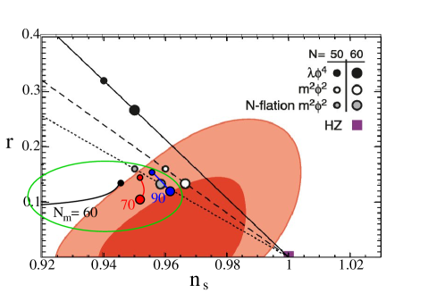
Figure 4: Predictions of chaotic inflation (and $N$-flation) and WMAP5 constraints for tensor ratio versus scalar spectral index. The predictions for the modified Friedmann equation are within the oval, for $N_{m}$ (the maximum number of $e$-foldings due to the energy density being bounded above by $\rho_{c}$) $=60$, 70 and 90. Each curve shows the evolution of the predicted $r,n_{s}$ as a function of number of e-foldings after horizon crossing, $N$, for $N=50$ to 60. Figure adapted from ref. [10].

Furthermore, the deviation of the standard single-field inflation consistency condition ${n_{t}/r}=-\frac{1}{8}$ of can be large; this is shown in figure 5. The magnitude depends on how close the value of the potential $V$ is to the maximum allowed value $V_{m}$ at horizon crossing of the relevant modes. Even though $n_{t}$ will be very difficult to measure with any accuracy, assuming that the tensor contribution $r$ will be observed, the discrepancy from the standard value for $V\cong V_{m}$ can be a factor of 3 or 4 without much fine tuning; in this case Planck should be able to detect it, despite the difficulty of measuring $n_{t}$ accurately.

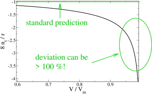
Figure 5: $8n_{t}/r$ versus $V/V_{m}$, showing deviation of braneworld prediction from the standard value, $-1$.

3 Nonlocal inflation and nongaussianity

It is well known that string theory predicts higher-derivative corrections to the effective action, including arbitrarily high orders in derivatives; these are known as $\alpha^{\prime}$ corrections. The usual procedure in string cosmology is to work in a low-energy regime where these corrections are small enough to safely ignore. However it is interesting to consider what can be said in the opposite regime. Normally this cannot be done in any reliable way because we do not know the $\alpha^{\prime}$ corrections to all orders. However, $p$-adic string theory provides an exception;$\!{}^{{\bf?}}$ in this theory the complete action is known to all orders,

$$S={m_{s}^{4}\over g_{s}^{2}}{p^{2}\over p-1}\int d^{\,26}x\left(-\frac{1}{2}\phi p^{-\Box/2m_{s}^{2}}\phi+{\phi^{p+1}\over p+1}\right)$$ (3)

where $m_{s}$ is the string scale, $g_{s}$ the string coupling, and $p$ = any prime number. The presence of derivatives at all orders makes it a nonlocal theory.

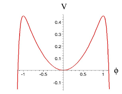
Figure 6: The potential of the tachyon of $p$-adic string theory.

The field $\phi$ is tachyonic at the maximum of its potential (fig. 6), $\phi=1$, where the curvature would normally be too great to support inflation. However in ref. [12] we found the surprising result that inflation from the maximum to the metastable minimum at $\phi=0$ can indeed occur in the regime where $\Box/m_{s}^{2}$ is not small. The Hubble scale $H$ is somewhat above $m_{s}$ for these solutions, which would normally mean that higher order corrections are out of control, but in the present case we have kept them to all orders.

3.1 Homogeneous solution

The Klein-Gordon equation and Friedmann equation are given by

$$e^{-\Box/m_{p}^{2}}\phi=\phi^{p},\qquad H^{2}={T_{00}\over 3M_{p}^{2}}$$ (4)

where $m_{p}^{2}\equiv{2m_{s}^{2}\over\ln p}$, and the energy density is given by a complicated expression

$$\rho_{\phi}=-T_{00}={m_{s}^{4}\over 2g_{p}^{2}}\left[\phi e^{-{\Box\over m_{p}^{2}}}\phi-{2\over p+1}\phi^{p+1}+{1\over m_{p}^{2}}\int_{0}^{1}d\tau\ \left(\Box e^{-{\tau\Box\over m_{p}^{2}}}\phi\right)\left(e^{-{(1-\tau)\Box\over m_{p}^{2}}}\phi\right)\right.$$

$$\left.+{1\over m_{p}^{2}}\int_{0}^{1}d\tau\ \partial_{t}\left(e^{-{\tau\Box\over m_{p}^{2}}}\phi\right)\partial_{t}\left(e^{-{(1-\tau)\Box\over m_{p}^{2}}}\phi\right)\right]$$ (5)

with ${1\over g_{p}^{2}}\equiv{1\over g_{s}^{2}}{p^{2}\over p-1}$. Nevertheless we can find approximate solutions when $\phi$ is near the top of the potential. When $H>m_{s}$, we can use the same friction-dominated approximation for the Laplacian as in ordinary inflation, $\Box=\partial^{2}_{t}+3H\partial_{t}\cong 3H_{0}\partial_{t}$. We find a solution of the form

$$\phi(t)=e^{-e^{\lambda t}},\quad\lambda\cong{2m_{s}^{2}\over 3H_{0}}$$ (6)

for which the energy density simplifies,

$$T_{00}(t)={m_{s}^{4}\over 2g_{s}^{2}}\,{p^{2}\over p-1}\left({p-1\over p+1}e^{-u(p+1)}+\int_{u}^{up}d\omega\,e^{-\omega-pu^{2}/\omega}\right)$$ (7)

The first term is potential and the second is kinetic energy. A striking difference between this and conventional inflationary solutions is the fact that slow roll of $\phi$ can occur while its energy is mainly kinetic; this is the case during the final stage of inflation. Fig. 7 shows the two contributions to $T_{00}$ and their sum as a function of time. For large values of $p$, the final, kinetic-dominated stage of inflation, can encompass all the observable $e$-foldings.

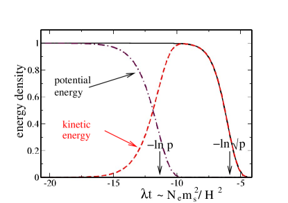
Figure 7: Energy density of $\phi$ versus time in $p$-adic inflation model, showing how the time of transition between potential and kinetic energy domination, and the time at which inflation ends, depend on $p$.

3.2 Fluctuations

For the spectrum of perturbations, we need to determine the fluctuations, $\phi\ =\ \phi_{0}(t)+\delta\phi(t,\vec{x})$. They obey the perturbed Klein-Gordon (KG) equation, $p^{-\Box/2m_{s}^{2}}\delta\phi=p\delta\phi$. This may at first look daunting, but it is easy to see that solutions of the usual KG equation $-\Box\delta\phi=\omega^{2}\delta\phi$ also satisfy the nonlocal one, provided that $\omega^{2}=2m_{s}^{2}$. However, $\delta\phi$ does not have a canonical kinetic term: it is of the form $-\frac{1}{2}\delta\phi F(\Box)\delta\phi$. One can do a field redefinition $\varphi=A\delta\phi\equiv(F(\Box)/\omega^{2})^{1/2}\delta\phi$ such that $\varphi$ does have a standard kinetic term (although its interactions will now become nonlocal). Using this field, one can assume the usual relation between the curvature perturbation and the inflaton fluctuation. It leads to the spectral index

$$n_{s}-1\ =\ 3-2\nu\ \cong\ -\frac{4}{3}\left(m_{s}\over H\right)^{2}\ \cong\ {8g_{s}^{2}\over p}\left(M_{p}\over m_{s}\right)^{2}$$ (8)

which shows the need for $H\gg m_{s}$ and $p\gg g_{s}^{2}$ to get $n_{s}=0.96$. The COBE normalization, $A_{\zeta}=5\times 10^{-5}$, puts a further constraint on $g_{s}^{2}/p$,

$${g_{s}\over\sqrt{p}}=\sqrt{8\over 3\pi^{2}}\,A_{\zeta}\,{e^{N_{e}|n_{s}-1|/2}\over|n_{s}-1|^{3/2}}\cong 2.5\times 10^{-7}$$ (9)

which depends on the observable number of $e$-foldings, $N_{e}$. These constraints together determine the string scale,

$$m_{s}\cong 3\times 10^{-7}M_{p}$$ (10)

3.3 Nongaussianity

One of the interesting features of the $p$-adic inflation is that for sufficiently large $p$, it predicts an observable level of nongaussianity, in contrast to conventional single-field inflation models.$\!{}^{{\bf?}}$ Heuristically this can be explained by the fact that the nongaussianity in single field models is suppressed by the slow roll parameters and by $V^{\prime\prime\prime}$; making $V^{\prime\prime\prime}(\phi_{0})$ large enough to compensate for the slow-roll suppression at some field value $\phi_{0}$ would spoil slow roll at nearby field values, before sufficient inflation could occur. However in nonlocal inflation, the fact that slow roll can continue despite a steep potential and kinetic energy domination gives a loophole. For large values of $p$, $V^{\prime\prime\prime}$ can be made sufficiently large for observable nongaussianity, yet remain compatible with 60 $e$-foldings of inflation.

Using the uniform curvature gauge in which tensor fluctuations are decoupled, the curvature perturbation is $\zeta=-{(H/\dot{\varphi}_{0})}\delta\varphi$, where $\varphi_{0}$ is the classical background solution. The bispectrum is then given by $\langle\zeta\zeta\zeta\rangle=-\left({H/\dot{\varphi}_{0}}\right)^{3}\langle\delta\varphi\,\delta\varphi\,\delta\varphi\rangle$. The three-point function for $\delta\varphi$ is related to the cubic term in the potential, $V_{\rm cubic}=2^{3/2}g_{s}m_{s}\delta\varphi^{3}$. Comparing to the definition of the nonlinearity parameter $f_{NL}$,

$$\langle\zeta_{k_{1}}\zeta_{k_{2}}\zeta_{k_{3}}\rangle=-\frac{3}{10}(2\pi)^{7}f_{NL}\,A_{\zeta}^{4}\,{{\scriptstyle\sum_{i}}k_{i}^{2}\over{\scriptstyle\prod_{i}}k_{i}^{3}}\,\delta^{(3)}({\scriptstyle\sum_{i}}\vec{k}_{i})$$ (11)

one can deduce that

$$f_{NL}\cong{5N_{e}\over 24\sqrt{2}}\,{\sqrt{p}\over\ln p}\,|n_{s}-1|^{2}e^{-N_{e}|n_{s}-1|/2}$$ (12)

in the $p$-adic inflation model. The nongaussianity turns out to be very nearly of the local form. Interesting values $30<f_{NL}<150$ as suggested by the analysis of ref. [14] can be obtained by taking $g_{s}\cong 0.1-0.25$ and $p\sim 10^{11}-10^{12}$.

References

References

- [1] J. Lesgourgues, “Features in the primordial power spectrum of double D-term inflation,” Nucl. Phys. B 582, 593 (2000) [arXiv:hep-ph/9911447].
- [2] L. Hoi, J. M. Cline and G. P. Holder, “Testing the Component in the Primordial Perturbation Power Spectrum,” arXiv:0706.3887 [astro-ph].
- [3] N. Barnaby and J. M. Cline, “Nongaussianity from tachyonic preheating in hybrid inflation,” Phys. Rev. D 75, 086004 (2007) [arXiv:astro-ph/0611750]. “Nongaussian and nonscale-invariant perturbations from tachyonic preheating in hybrid inflation,” Phys. Rev. D 73, 106012 (2006) [arXiv:astro-ph/0601481].
- [4] J. O. Gong and M. Sasaki, “Curvature perturbation spectrum from false vacuum inflation,” arXiv:0804.4488 [astro-ph].
- [5] J. H. Traschen, “Constraints on Stress Energy Perturbations in General Relativity,” Phys. Rev. D 31, 283 (1985); “Causal Cosmological Perturbations and Implications for the Sachs-Wolfe Effect,” Phys. Rev. D 29, 1563 (1984).
- [6] F. Chen, J. M. Cline and S. Kanno, “Modified Friedmann Equation and Inflation in Warped Codimension-two Braneworld,” Phys. Rev. D 77, 063531 (2008) [arXiv:0801.0226 [hep-th]].
- [7] L. Randall and R. Sundrum, “A large mass hierarchy from a small extra dimension,” Phys. Rev. Lett. 83, 3370 (1999) [arXiv:hep-ph/9905221].
- [8] G. R. Dvali, G. Gabadadze and M. Porrati, “4D gravity on a brane in 5D Minkowski space,” Phys. Lett. B 485, 208 (2000) [arXiv:hep-th/0005016].
- [9] J. M. Cline, J. Descheneau, M. Giovannini and J. Vinet, “Cosmology of codimension-two braneworlds,” JHEP 0306, 048 (2003) [arXiv:hep-th/0304147].
- [10] D. N. Spergel et al. [WMAP Collaboration], “Wilkinson Microwave Anisotropy Probe (WMAP) three year results: Implications for cosmology,” Astrophys. J. Suppl. 170, 377 (2007) [arXiv:astro-ph/0603449].
- [11] P. G. O. Freund and M. Olson, “Nonarchimedean strings,” Phys. Lett. B 199, 186 (1987); P. G. O. Freund and E. Witten, “Adelic string amplitudes,” Phys. Lett. B 199, 191 (1987). L. Brekke, P.G. Freud, M. Olson and E. Witten, “Nonarchimedean String Dynamics,” Nucl. Phys. B 302, 365 (1998).
- [12] N. Barnaby, T. Biswas and J. M. Cline, “p-adic inflation,” JHEP 0704, 056 (2007) [arXiv:hep-th/0612230].
- [13] N. Barnaby and J. M. Cline, “Large Nongaussianity from Nonlocal Inflation,” JCAP 0707, 017 (2007) [arXiv:0704.3426 [hep-th]]; “Predictions for Nongaussianity from Nonlocal Inflation,” arXiv:0802.3218 [hep-th].
- [14] A. P. S. Yadav and B. D. Wandelt, “Detection of primordial non-Gaussianity (fNL) in the WMAP 3-year data at above 99.5arXiv:0712.1148 [astro-ph].