BETHE-Hydro: An Arbitrary Lagrangian-Eulerian Multi-dimensional Hydrodynamics Code for Astrophysical Simulations

Abstract

In this paper, we describe a new hydrodynamics code for 1D and 2D astrophysical simulations, BETHE-hydro, that uses time-dependent, arbitrary, unstructured grids. The core of the hydrodynamics algorithm is an arbitrary Lagrangian-Eulerian (ALE) approach, in which the gradient and divergence operators are made compatible using the support-operator method. We present 1D and 2D gravity solvers that are finite differenced using the support-operator technique, and the resulting system of linear equations are solved using the tridiagonal method for 1D simulations and an iterative multigrid-preconditioned conjugate-gradient method for 2D simulations. Rotational terms are included for 2D calculations using cylindrical coordinates. We document an incompatibility between a subcell pressure algorithm to suppress hourglass motions and the subcell remapping algorithm and present a modified subcell pressure scheme that avoids this problem. Strengths of this code include a straightforward structure, enabling simple inclusion of additional physics packages, the ability to use a general equation of state, and most importantly, the ability to solve self-gravitating hydrodynamic flows on time-dependent, arbitrary grids. In what follows, we describe in detail the numerical techniques employed and, with a large suite of tests, demonstrate that BETHE-hydro finds accurate solutions with 2^nd-order convergence.

1. Introduction

The ability to simulate hydrodynamic flow is key to studying most astrophysical objects. Supernova explosions, gamma-ray bursts, X-ray bursts, classical novae, the outbursts of luminous blue variables (LBVs), and stellar winds are just a few phenomena for which understanding and numerical tools evolve in tandem. This is due in part to the physical complexity, multi-dimensional character, and instabilities of such dynamical fluids. Moreover, rotation is frequently a factor in the dynamical development of astrophysical transients. One-dimensional hydrodynamics is by and large a solved problem, but multi-dimensional hydrodynamics is still a challenge. In the context of astrophysical theory, this is due primarily to the need to address time-dependent gravitational potentials, complicated equations of state (EOSs), flexible grids, multi-D shock structures, and chaotic and turbulent flows. As a result, theorists who aim to understand the Universe devote much of their time to code development and testing.

One of the outstanding and complex problems in theoretical astrophysics is the mechanism for core-collapse supernovae. For more than two decades, the preferred mechanism of explosion has been the delayed neutrino mechanism (Bethe & Wilson, 1985). One-dimensional (1D) simulations generally fail to produce explosions (Liebendörfer et al., 2001b, a; Rampp & Janka, 2002; Buras et al., 2003; Thompson et al., 2003; Liebendörfer et al., 2005). However, 2-dimensional (2D) simulations, and the accompanying aspherical instabilities, suggest that the neutrino-mechanism may indeed be viable (Herant et al., 1994; Janka & Mueller, 1995; Burrows et al., 1995, 2007b; Buras et al., 2006; Kitaura et al., 2006), though this has yet to be proven. In fact, Burrows et al. (2006) have recently reported an acoustic mechanism, which seems to succeed on long timescales when and if other mechanisms fail. These authors identified two primary reasons why this mechanism might have been missed before: 1) 2D radiation-hydrodynamic simulations with reasonable approximations are still expensive to run, and with limited resources simulations are rarely carried to late enough times; and 2), a noteworthy feature of the code they used, VULCAN/2D, is its Arbitrary Lagrangian-Eulerian (ALE) structure. VULCAN/2D incorporates non-standard grids that liberate the inner core from the Courant and resolution limitations of standard spherical grids. In this context, Burrows et al. (2006) claim that simulating all degrees of freedom leads to a new mechanism in which the gravitational energy in aspherical accretion is converted to explosion energy by first exciting protoneutron star core g-modes. These modes then radiate acoustic power and revive the stalled shock into explosion. Remarkably, the acoustic mechanism, given enough time, leads to successful core-collapse supernovae in all progenitors more massive than $\sim$9 M_⊙ simulated to date (Burrows et al., 2006, 2007b). However, this is a remarkable claim, and given the implications, must be thoroughly investigated. For instance, one question to ask is: could the results seen by Burrows et al. (2006) be numerical artifacts of VULCAN?

Therefore, to address this and other issues that surround the acoustic supernova mechanism, as well as a host of other outstanding astrophysical puzzles, we have designed the new hydrodynamic code, BETHE-hydro, from the bottom up. BETHE-hydro will be coupled with the 2D mixed-frame radiation transport scheme of Hubeny & Burrows (2007) to create the 2D radiation/hydrodynamics code BETHE, and the merger of these two codes will be the subject of a future paper. In this paper, we present and test the hydrodynamic and gravity algorithms of BETHE-hydro. Since BETHE-hydro uses arbitrary grids and a general gravity solver, we expect it to be a powerful and flexible numerical tool, able to configure the grid to suit the computational challenge.

The core of BETHE-hydro is a 1D and 2D ALE hydrodynamics solver. First, solutions to the Lagrangian hydrodynamic equations are obtained on an arbitrary polygonal grid. Then, to avoid tangled grids, the hydrodynamic variables can be remapped to another grid. A unique and powerful feature of ALE schemes is their flexibility to tailor an arbitrary grid to the computational challenge and to alter the grid dynamically during runtime. Hence, purely Lagrangian, purely Eulerian, or arbitrarily moving grids (chosen to optimize numerical performance and resolution) are possible. These grids can be non-orthogonal, non-spherical, and non-Cartesian.

Some of the earliest 2D hydrodynamic simulations in astrophysics were, in fact, performed to address the core-collapse problem. While some employed standard fixed-grid schemes (Smarr et al., 1981), other 2D simulations were calculated with adaptive grids. Although many utilized moving grids, for the most part, the differencing formulations were Eulerian (LeBlanc & Wilson, 1970; Symbalisty, 1984; Miller et al., 1993). On the other hand, Livio et al. (1980) did employ an “Euler-Lagrange” method involving a Lagrangian hydrodynamic solve, followed by a remapping stage. Even though these simulations did exploit radially dynamical grids, they were restricted to be orthogonal and spherical.

Many of the current hydrodynamic algorithms used in astrophysics are based upon either ZEUS (Stone & Norman, 1992) or higher-order Godunov methods, in particular the Piecewise-Parabolic Method (PPM) (Colella & Woodward, 1984; Woodward & Colella, 1984). Both approaches have been limited to orthogonal grids. One concern with PPM-based codes is that they solve the hydrodynamic equations in dimensionally-split fashion. As a result, there have been concerns that these algorithms do not adequately resolve flows that are oblique to the grid orientation. Rectifying this concern, recent unsplit higher-order Godunov schemes, or approximations thereof, have been developed (Truelove et al., 1998; Klein, 1999; Gardiner & Stone, 2005; Miniati & Colella, 2007). Despite this and the employment of adaptive mesh refinement (AMR), these codes must use orthogonal grids that are often strictly Cartesian.

In BETHE-hydro, we use finite-difference schemes based upon the support-operator method (Shashkov & Steinberg, 1995) of Caramana et al. (1998) and Caramana & Shashkov (1998). Differencing by this technique enables conservation of energy to roundoff error in the absence of rotation and time-varying gravitational potentials. Similarly, momentum is conserved accurately, but due to the artificial viscosity scheme that we employ, it is conserved to roundoff error for hydrodynamic simulations using Cartesian coordinates only. Moreover, using the support-operator method and borrowing from an adaptation of the support-operator technique for elliptic equations (Morel et al., 1998), we have developed a gravity solver for arbitrary grids. Unfortunately, by including a general gravity capability, we sacrifice strict energy and momentum conservation. However, we have performed tests and for most cases the results are reasonably accurate. Furthermore, we have included rotational terms and we use a modified version of the subcell pressure scheme to mitigate hourglass instabilities (Caramana & Shashkov, 1998).

To resolve shocks, we employ an artificial viscosity method, which is designed to maintain grid stability as well (Campbell & Shashkov, 2001), and there are no restrictive assumptions made about the equation of state. Higher-order Godunov techniques employ Riemann solvers to resolve shocks, but frequently need an artificial viscosity scheme to eliminate unwanted post-shock ringing. Moreover, the inner workings of Riemann solvers often make local approximations that the EOS has a gamma-law form, which stipulates that as the internal energy goes to zero so does the pressure. For equations of state appropriate for core-collapse supernovae, this artificially imposed zero-point energy can pose problems for the simulations (Buras et al., 2006).

Two codes in astrophysics which have already capitalized on the arbitrary grid formulations of ALE are Djehuty (Bazán et al., 2003; Dearborn et al., 2005) and VULCAN/2D (Livne, 1993; Livne et al., 2004). In both cases, the grids employed were designed to be spherical in the outer regions, but to transition smoothly to a cylindrical grid near the center. These grid geometries reflected the basic structure of stars, while avoiding the cumbersome singularity of a spherical grid. With this philosophy, Dearborn et al. (2006), using Djehuty, have studied the helium core flash phase of stellar evolution in 3D. In the core-collapse context, Burrows et al. (2006, 2007a, 2007b), using VULCAN/2D, performed 2D radiation/hydrodynamic and radiation/MHD simulations with rotation.

Several gravity solvers have been employed in astrophysics. The most trivial are static or monopole approaches. For arbitrary potentials, the most extensively used are N-body schemes, which fit most naturally in Smooth Particle Hydrodynamics (SPH) codes (Monaghan, 1992). As a virtue, SPH solves the equations in a grid-free context, and while SPH has opened the way to three-dimensional (3D) hydrodynamic simulations in astrophysics, including core-collapse simulations (Fryer & Warren, 2002), the smoothing kernels currently employed pose serious problems for simulating fundamental hydrodynamic instabilities such as the Kelvin-Helmholtz instability (Agertz et al., 2007). Another approach to the solution of Poisson’s equation for gravity is the use of multipole expansions of the potential (Müller & Steinmetz, 1995). This technique achieves its relative speed by calculating simple integrals on a spherical grid once. Then, the stored integrals are used in subsequent timesteps. In BETHE-hydro, we construct finite-difference equations for Poisson’s equation using the support-operator method and find solutions to the resulting linear system of equations for the potentials via an iterative multigrid-preconditioned conjugate-gradient method (Ruge & Stuben, 1987).

In §2, we give a summary of BETHE-hydro and sketch the flowchart of the algorithm. The coordinates and mesh details are discussed in §3. We then describe in §4 the discrete Lagrangian equations, including specifics of the 2^nd-order time-integration and rotational terms. Section 5 gives a complete description of the 1D and 2D gravity solvers. Hydrodynamic boundary conditions are discussed in §6. The artificial viscosity algorithm that provides shock resolution and grid stability is described in §7. In §8, we present the subcell pressure scheme that suppresses hourglass modes. Remapping is described in depth in §9. In §10, we demonstrate the code’s strengths and limitations with some test problems. Finally, in §11 we summarize the central characteristics and advantages of BETHE-hydro.

2. BETHE-Hydro: An Arbitrary Lagrangian-Eulerian Code

In ALE algorithms, the equations of hydrodynamics are solved in Lagrangian form. Within this framework, equations for the conservation of mass, momentum, and energy are:

$$\frac{d\rho}{dt}=-\rho\vec{\nabla}\cdot\vec{v}\,,$$ (1)

$$\rho\frac{d\vec{v}}{dt}=-\rho\vec{\nabla}\Phi-\vec{\nabla}P\,,$$ (2)

and

$$\rho\frac{d\varepsilon}{dt}=-P\vec{\nabla}\cdot\vec{v}\,.$$ (3)

$\rho$ is the mass density (which we refer to simply as “density” and is distinct from the energy or momentum densities), $\vec{v}$ is the fluid velocity, $\Phi$ is the gravitational potential, $P$ is the isotropic pressure, $\varepsilon$ is the specific internal energy, and $d/dt=\partial/\partial t+\vec{v}\cdot\vec{\nabla}$ is the Lagrangian time derivative. The equation of state may have the following general form:

$$P=P(\rho,\varepsilon,X_{i})\,,$$ (4)

where $X_{i}$ denotes the mass fraction of species $i$. Therefore, we also solve the conservation equations:

$$\frac{dX_{i}}{dt}=0\,.$$ (5)

Completing the set of equations for self-gravitating astrophysical flows is Poisson’s equation for gravity:

$$\nabla^{2}\Phi=4\pi G\rho\,,$$ (6)

where $G$ is Newton’s gravitational constant.

All ALE methods have the potential to solve eqs. (1-3) using arbitrary, unstructured grids. In this lies the power and functionality of ALE methods. The solutions involve two steps and are conceptually quite simple: 1) a Lagrangian solver moves the nodes of the mesh in response to the hydrodynamic forces; and 2) to avoid grid tangling, the nodes are repositioned, and a remapping algorithm interpolates hydrodynamic quantities from the old grid to this new grid. Of course, the challenge is to find accurate solutions, while conserving energy and momentum. In constructing BETHE-hydro to satisfy these requirements, we use the ALE hydrodynamic techniques of Caramana et al. (1998), Caramana & Shashkov (1998), Campbell & Shashkov (2001), and Loubère & Shashkov (2005).

To summarize the overall structure of BETHE-hydro, we present a schematic flowchart, Fig. 1, and briefly describe the key steps. Establishing the structure for all subsequent routines, the first step is to construct the arbitrary, unstructured grid. This leads to the next step, problem initialization. Then, the main loop for timestep integration is entered. After a call to the EOS to obtain the pressure, solutions to Poisson’s equation for gravity are calculated using either the 2D or 1D algorithms in §5. Both use the support-operator method to discretize eq. (6), and the resulting system of linear equations is solved by a tridiagonal solver in 1D and a multigrid pre-conditioned conjugate-gradient iterative method in 2D (§5).

After the timestep is calculated (§4.2), the Lagrangian equations of hydrodynamics are solved on an arbitrary grid using the compatible hydrodynamics algorithm of Caramana et al. (1998) (see §4 for further discussion). To ensure 2nd-order accuracy in both space and time, we employ a predictor-corrector iteration (§4.2), in which a second call to the EOS and the gravity solver are required. Other than the gravity solver block, the Lagrangian hydrodynamics solver (§4) is represented by the set of steps beginning with Predictor and ending with Corrector (Fig. 1).

After finding Lagrangian hydrodynamic solutions at each timestep, one could proceed directly to the next timestep, maintaining the Lagrangian character throughout the simulation. However, in multiple spatial dimensions, grid tangling will corrupt flows with significant vorticity. In these circumstances, we conservatively remap the Lagrangian solution to a new arbitrary grid that mitigates tangled grids. The new grid may be the original grid, in which case we are solving the hydrodynamic equations in the Eulerian frame, or it may be a new, arbitrarily-defined, grid.

3. Coordinate Systems and Mesh

In BETHE-hydro, eqs. (1-6) may be solved with any of several coordinate systems and assumed symmetries. Included are the standard 1D & 2D Cartesian coordinate systems. For astrophysical applications, we use 1D spherical and 2D cylindrical coordinate systems. Irrespective of the coordinate system, we indicate a position by $\vec{x}$. The components of the Cartesian coordinate system are $x$ and $y$; the spherical components are $r$, $\theta$, and $\phi$; and the cylindrical coordinates are $r$, $z$, and $\phi$.

Distinct from the coordinate system is the grid, or mesh, which defines an arbitrary discretization of space. It is this unique feature and foundation of ALE techniques that provides their flexibility. Figure 2 shows two example grids: the butterfly mesh on the left and a spiderweb mesh on the right. Either may be used in a 2D Cartesian or 2D cylindrical simulations, although the placement of the nodes is neither Cartesian nor cylindrical. Instead, these meshes have been designed to simulate spherically or cylindrically convergent phenomena without the limitation of small zones near the center.

When using cylindrical coordinates in ALE algorithms, one may use control-volume differencing (CVD) or area-weighted differencing (AWD); we use CVD. Thorough comparisons of these two differencing schemes may be found in Caramana et al. (1998). Here, we give a basic justification for choosing CVD. For CVD, the volumes of the subcell, cell, and node are calculated by straightforward partitioning of these regions by edges. Hence, volumes and masses are exact representations of their respective regions. While this discretization is natural and easy to comprehend, it does not preserve strict spherical symmetry when using a spherical grid and cylindrical coordinates. On the other hand, AWD is designed to preserve spherically symmetric flows, but only with the use of spherical grids that have equal spacing in angle. Since this prevents the use of arbitrary grids, and the asymmetries of CVD are small, we use CVD for discretization.

Construction of the grid begins with the arbitrary placement of nodes. At these nodes, coordinate positions, velocities, and accelerations are defined. Simply specifying node locations does not completely define a mesh, since there is not a unique way to assign cells and masses to these nodes. Therefore, the user must specify the connectivity among nodes, which define the arbitrarily-shaped polygonal cells. It is within these cells that cell-centered averages of $\rho$, $\varepsilon$, $P$, $X_{i}$, and $\Phi$ are defined.

With the node positions, their connectivity, and the cells defined, a mesh is completely specified and all other useful descriptions follow. Cells are denoted by $z$, and nodes are indexed by $p$. The set of nodes that defines cell $z$ are $p\in S(z)$, where the nodes are ordered counterclockwise. Conversely, the set of cells that shares node $p$ is denoted by $z\in S(p)$. Each cell has $N_{p}(z)$ nodes that define it, and each node has $N_{z}(p)$ cells that share it. The sample sub-grid depicted in Fig. 3 helps to illustrate the nodal and cell structure. The filled circles indicate node positions, $\vec{x}_{p}$, and the crosses indicate the cell-center positions, $\vec{x}_{z}=(1/N_{p}(z))\sum_{p\in S(z)}\vec{x}_{p}$. The solid lines are direction-oriented edges that separate cells from one another, and the open circles indicate their mid-edge locations. Partitioning the cell into subcells, the dashed lines connect the mid-edges with the cell centers. No matter how many sides a cell has, with this particular division the subcells are always quadrilaterals. Naturally, the cell volumes (see appendix B for formulae calculating discrete volumes), $V_{z}$, are related to the subcell volumes, $V^{z}_{p}$, by

$$V_{z}=\sum_{p\in S(z)}V^{z}_{p}\,.$$ (7)

Furthermore, each node has a volume, $V_{p}$, defined by the adjoining subcells that share the node $p$:

$$V_{p}=\sum_{z\in S(p)}V^{p}_{z}\,.$$ (8)

For calculating pressure forces and fluxes, vectors are assigned to each half edge on either side of node $p$: $\vec{C}^{z}_{p+}$ and $\vec{C}^{z}_{p-}$, where $+$ indicates the half edge in the counterclockwise direction around the cell and $-$ indicates its opposite counterpart. Their magnitudes are the areas represented by the half edges, and their directions point outward and normal to the surface of cell $z$. From these half-edge area vectors, an area vector, $\vec{S}^{z}_{p}$, that is associated with zone $z$ and node $p$ is then defined:

$$\vec{S}^{z}_{p}=\vec{C}^{z}_{p+}+\vec{C}^{z}_{p-}\,.$$ (9)

Similarly, vectors are associated with the lines connecting the mid-edges and the cell centers: $\vec{a}^{z}_{p}$. Again, their magnitudes are the corresponding area, but while the vector is normal to this line, the direction is oriented counterclockwise around the cell.

4. Discrete Lagrangian Hydrodynamics

The fundamental assumption of Lagrangian algorithms is that the mass, $m_{z}$, of a discrete volume $V_{z}$ is constant with time. For staggered-grid methods, in which scalars are defined as cell-centered averages and vectors are defined at the nodes, it is necessary to define a Lagrangian mass, $m_{p}$, for the nodes as well. This nodal mass is associated with the node’s volume $V_{p}$ (eq. 8). Conservation of mass (eq. 1) implies zero mass flux across the boundaries, $\partial V$, of either the cell volume or nodal volume. Therefore, the region of overlap for $V_{z}$ and $V_{p}$, which is the subcell volume $V^{z}_{p}$, is bounded by surfaces with zero mass flux. Consequently, the most elemental Lagrangian mass is the subcell mass, $m^{z}_{p}$, and the cell mass ($m_{z}$) and node mass ($m_{p}$) are constructed as appropriate sums of subcell masses:

$$m_{z}=\sum_{p\in S(z)}m^{z}_{p}\,,$$ (10)

and

$$m_{p}=\sum_{z\in S(p)}m^{p}_{z}\,.$$ (11)

Hence, we arrive at three discrete forms of mass conservation (eq. 1):

$$\begin{array}[]{cccc}\rho^{z}_{p}=\frac{m^{z}_{p}}{V^{z}_{p}}\,,&\rho_{p}=\frac{m_{p}}{V_{p}}\,,&\mbox{and}&\rho_{z}=\frac{m_{z}}{V_{z}}\,.\end{array}$$ (12)

In defining the discrete momentum and energy equations, we use the compatible hydrodynamics algorithms developed by Caramana et al. (1998). Specifically, the discrete divergence and gradient operators are compatible in that they faithfully represent their analog in continuous space and their definitions are expressly related to one another using the hydrodynamic expressions for conservation of momentum and energy. As a result, this approach leads to discretizations that satisfy momentum and energy conservation to machine accuracy. This is accomplished with the support-operator method (Shashkov & Steinberg, 1995). Given the integral identity,

$$\int_{V}\Phi(\vec{\nabla}\cdot\vec{H})dV+\int_{V}\vec{H}\cdot\vec{\nabla}\Phi dV=\oint_{\partial V}\Phi\vec{H}\cdot d\vec{S}\,,$$ (13)

where $\Phi$ is any scalar and $\vec{H}$ is some vector, there is an incontrovertible connection between the divergence and gradient operators. For many choices of discretization, the discrete counterparts of these operators could violate this integral identity. Simply put, the goal of the support-operator method is to define the discrete operators so that they satisfy eq. (13). The first step is to define one of the discrete operators. It is often, but not necessary, that the discrete divergence operator is defined via Gauss’s Law:

$$\int_{V}\vec{\nabla}\cdot\vec{v}dV=\oint_{\partial V}\vec{v}\cdot d\vec{S}\,,$$ (14)

and then eq. (13) is used to compatibly define the other discrete operator. Discretizing the hydrodynamic equations, Caramana et al. (1998) begin by defining $(\vec{\nabla}P)_{p}$ at the nodes and use the integral form of energy conservation and an equation equivalent to eq. (13) to define for each cell the discrete divergence of the velocity, $(\vec{\nabla}\cdot\vec{v})_{z}$.

To begin, Caramana et al. (1998) integrate eq. (2) (excluding gravity and rotational terms) over the volume of node $p$, producing the discrete form for $(\vec{\nabla P})_{p}$ and the momentum equation:

$$m_{p}\frac{\Delta\vec{v}_{p}}{\Delta t} = -\int_{V_{p}}\vec{\nabla}P\,dV$$ (15)

$$= -\oint_{\partial V_{p}}P\,d\vec{S}$$

$$= -\sum_{z\in S(p)}P_{z}\vec{S^{p}_{z}}\,,$$

where $\Delta\vec{v}_{p}=\vec{v}_{p}^{n+1}-\vec{v}^{n}_{p}$ is the change in velocity from timestep $n$ to the next timestep $n+1$, the timestep is $\Delta t$, and $P_{z}$ is the pressure in cell $z$. In other words, the net force on node $p$ is a sum of the pressure times the directed zone areas that share node $p$. Hence, the subcell force exerted by zone $z$ on point $p$ is $\vec{f}^{p}_{z}=P_{z}\vec{S}^{p}_{z}$. A more complete description of the subcell force, however, must account for artificial viscosity (§7):

$$\vec{f}^{p}_{z}=P_{z}\vec{S}^{p}_{z}+\vec{f}^{p}_{z,\rm{visc}}\,,$$ (16)

where $\vec{f}^{p}_{z,\rm{visc}},$ is the subcell force due to artificial viscosity. Furthermore, in this work, we include gravity and rotation for 2D axisymmetric simulations, and the full discrete momentum equation becomes

$$m_{p}\frac{\Delta\vec{v}_{p}}{\Delta t}=\sum_{z\in S(p)}\vec{f}^{p}_{z}+m_{p}\vec{g}_{p}+m_{p}\vec{A}_{p}\,,$$ (17)

where $\vec{g}_{p}$ and $\vec{A}_{p}$ are the gravitational and rotational accelerations, respectively. For simplicity, and to parallel the discussion in Caramana et al. (1998), we ignore these terms in the momentum equation and proceed with the compatible construction of the energy equation (see §4.3.1 and §5.4 for discussions of total energy conservation including rotation and gravity, respectively).

To construct the discrete energy equation, Caramana et al. (1998) integrate eq. (3) over the discrete volume of cell $z$:

$$m_{z}\frac{\Delta\varepsilon_{z}}{\Delta t}=-\int_{V_{z}}P\vec{\nabla}\cdot\vec{v}\,dV=-P_{z}(\vec{\nabla}\cdot\vec{v})_{z}V_{z}\,,$$ (18)

where $\Delta\varepsilon_{z}=\varepsilon_{z}^{n+1}-\varepsilon_{z}^{n}$. Then, the objective is to determine a discrete form for the right hand side of this equation that conserves energy and makes the discrete gradient and divergence operators compatible. Caramana et al. (1998) accomplish this with the integral for conservation of energy (neglecting gravity):

$$\int\left(\rho\frac{d\varepsilon}{dt}+\frac{1}{2}\rho\frac{dv^{2}}{dt}\right)dV = -\int_{V}(P\vec{\nabla}\cdot\vec{v}+\vec{v}\cdot\vec{\nabla}P)dV$$ (19)

$$= -\oint_{\partial V}P\vec{v}\cdot d\vec{S}\,,$$

where the second expression is the integral identity, eq. (13), that defines the physical relationship between the gradient and divergence operators. Neglecting boundary terms, the discrete form of this integral is

$$\sum_{z}\left(m_{z}\frac{\Delta\varepsilon_{z}}{\Delta t}+\sum_{p\in S(z)}\vec{v}^{n+1/2}_{p}\cdot\vec{f}^{p}_{z}\right)=0\,,$$ (20)

where we used $\Delta\vec{v}^{2}_{p}=(\vec{v}^{n+1}_{p})^{2}-(\vec{v}^{n}_{p})^{2}=2\vec{v}^{n+1/2}_{p}\cdot\Delta\vec{v}_{p}$, $\vec{v}^{n+1/2}_{p}=1/2(\vec{v}^{n+1}_{p}+\vec{v}^{n}_{p})$, and substituted in eq. (15). If we set the expression for each zone in eq. (20) to zero, we arrive at the compatible energy equation:

$$m_{z}\frac{\Delta\varepsilon_{z}}{\Delta t}=-\sum_{p\in S(z)}\vec{v}^{n+1/2}_{p}\cdot\vec{f}^{z}_{p}\,.$$ (21)

The RHS of eq. (21) is merely the $PdV$ work term of the first law of thermodynamics. Its unconventional form is a consequence of the support-operator method.

Thus, we derive two significant results. First, inspection of eqs. (21) and (15) leads to compatible definitions for the discrete gradient and divergence operators. Specifically, the discrete analogs of the gradient and divergence operators are

$$(\vec{\nabla}P)_{p}=\frac{1}{V_{p}}\sum_{z\in S(p)}P_{z}\vec{S}^{p}_{z}$$ (22)

and

$$(\vec{\nabla}\cdot\vec{v})_{z}=\frac{1}{V_{z}}\sum_{p\in S(z)}\vec{v}_{p}\cdot\vec{S}^{p}_{z}\,.$$ (23)

Second, eqs. (12), (15), and (21) form the compatible discrete equations of Lagrangian hydrodynamics.

4.1. Momentum Conservation

In its current form, BETHE-hydro strictly conserves momentum for simulations that use Cartesian coordinates and not cylindrical coordinates. Caramana et al. (1998) show that the requirement for strict conservation is the use of control-volume differencing, or that exact representations of cell surfaces are employed. As a simple example, consider momentum conservation with pressure forces only:

$$\sum_{p}\vec{F}_{p}=\sum_{p}\sum_{z\in S(p)}\vec{f}^{p}_{z}=\sum_{z}P_{z}\sum_{p\in S(z)}\vec{S}^{z}_{p}\,.$$ (24)

For Cartesian coordinates, the sum $\sum_{p\in S(z)}\vec{S}^{z}_{p}$ is exactly zero for each cell as long as the surface-area vectors are exact representations of the cell’s surface. This is not the case for area-weighted differencing, and hence momentum is not conserved in that case. For cylindrical coordinates, the sum of surface-area vectors gives zero only for the $z$-component. However, the assumption of symmetry about the cylindrical axis ensures momentum conservation for the $r$-component. Therefore, control-volume differencing ensures momentum conservation, even with the use of cylindrical coordinates.

Based upon similar arguments, the subcell-pressure forces that eliminate hourglass motions (§8) are formulated to conserve momentum for both Cartesian and cylindrical coordinates. On the other hand, because we multiply the Cartesian artificial viscosity force by $2\pi r_{p}$ to obtain the force appropriate for cylindrical coordinates, the artificial viscosity scheme (§7) that we employ is conservative for Cartesian coordinates only.

We test momentum conservation with the Sedov blast wave problem (§10.3) using Cartesian and cylindrical coordinates. Symmetry dictates conservation in the $r$-component of the momentum. Consequently, we compare the $z$-component of the total momentum at $t=0$ s with subsequent times. Since the initial momentum of this test is zero, we obtain a relative error in momentum by $P_{z}(t)/P_{z,z>0}(t)$, where $P_{z}(t)$ is the $z$-component of the total momentum at time $t$ and $P_{z,z>0}(t)$ is a similar quantity for $z>0$. As expected, the relative error using Cartesian coordinates reflects roundoff error. For cylindrical coordinates and 35,000 cells, the relative error in momentum is $\sim 3\times 10^{-7}$ after 0.8 s and 71,631 timesteps. Although momentum is strictly conserved for simulations using Cartesian coordinates only, the Sedov blast wave problem demonstrates that momentum is conserved very accurately, even when cylindrical coordinates are used.

4.2. Second-Order Time Integration: Predictor-Corrector

Our method is explicit in time. Therefore, for numerical convergence, we limit the timestep, $\Delta t$, to be smaller than three timescales. By the Courant-Friedrichs-Levy (CFL) condition we limit $\Delta t$ to be smaller than the shortest sound-crossing time and the time it takes flow to traverse a cell. The latter condition is useful to avoid tangled meshes and is necessary when remapping is used. In addition, it is limited to be smaller than the fractional change in the volume represented by $(\vec{\nabla}\cdot\vec{v})_{z}$. In calculating these timescales a characteristic length for each cell is needed. Given arbitrary polygonal grids, we simply use the shortest edge for each cell. In practice, the timestep is the shortest of these timescales multiplied by a scaling factor, CFL. In our calculations, we set ${\rm CFL}=0.25$.

To ensure second-order accuracy and consistency with the time levels specified in eqs. (17) and (21), we employ predictor-corrector time integration using the finite difference stencil from Caramana et al. (1998). For each timestep, the current time level of each quantity is identified with $n$ in superscript. The time-centered quantities are indicated with a $n+1/2$ superscript, while the predicted values are labeled $n+1,pr$, and the fully updated values for the next timestep are labeled with a $n+1$ superscript.

Table 1 lists the steps for the predictor-corrector integration. The predictor step begins by defining the forces on nodes, $\vec{f}^{n}$, using current pressures $P^{n}$, areas $\vec{S}^{n}$, and artificial viscosity forces $\vec{f}^{n}_{\rm{visc}}$. Eq. (17) is then used to calculate the predicted velocity, $\vec{v}^{n+1,pr}$. The predicted node coordinate is then calculated by $\vec{x}^{n+1,pr}=\vec{x}^{n}+\Delta t\vec{v}^{n+1/2}$, where $\vec{v}^{n+1/2}$ is the time-centered velocity computed as $\vec{v}^{n+1/2}=\frac{1}{2}(\vec{v}^{n+1,pr}+\vec{v}^{n})$. Then, using $\vec{f}^{n}$ and $\vec{v}^{n+1/2}$ in eq. (21), the predicted specific internal energy, $\varepsilon^{n+1,pr}$, is obtained. Using the predicted node positions, the predicted rotational acceleration ($\vec{A}^{n+1,pr}_{p}$), volume ($V^{n+1,pr}$), and density ($\rho^{n+1,pr}$), are computed, which in turn are used to calculate the predicted gravitational acceleration, $\vec{g}^{n+1,pr}$. Calling the EOS with $\varepsilon^{n+1,pr}$ and $\rho^{n+1,pr}$ gives the predicted pressure $P^{n+1,pr}$. We finish the predictor step and prepare for the corrector step by calculating the time-centered positions $\vec{x}^{n+1/2}$, pressures $P^{n+1/2}$, rotational accelerations $\vec{A}^{n+1/2}_{p}$, and gravitational accelerations $\vec{g}^{n+1/2}$ as simple averages of their values at the $(n+1,pr)$ and $n$ time levels.

The corrector step then proceeds similarly to the predictor step. $P^{n+1/2}$ and $\vec{S}^{n+1/2}$ are used to compute $\vec{f}^{n+1/2}$, which in turn is used to compute the updated velocity, $\vec{v}^{n+1}$. After computing the new time-centered velocity, the node coordinates are finally updated using the time-centered velocity. Then, the specific internal energy, $\varepsilon^{n+1/2}$, is updated using $\vec{f}^{n+1/2}$ and $\vec{v}^{n+1/2}$. Finally, the volume, $V^{n+1}$, and density $\rho^{n+1}$ are computed for the next timestep.

4.3. Rotation in 2D cylindrical coordinates

In 2D simulations using cylindrical coordinates, we have extended BETHE-hydro to include rotation about the axis of symmetry. For azimuthally symmetric configurations, all partial derivatives involving $\phi$ are zero. Consequently, the conservation of mass and energy equations are

$$\frac{D\rho}{Dt}=-\rho\vec{\nabla}_{rz}\cdot\vec{v}$$ (25)

and

$$\rho\frac{D\varepsilon}{Dt}=-P\vec{\nabla}_{rz}\cdot\vec{v}\,,$$ (26)

where the $rz$ subscript on the del operator reminds us that the derivatives with respect to $\phi$ vanish. For concise notation, we define a pseudo Lagrangian derivative:

$$\frac{D}{Dt}=\frac{\partial}{\partial t}+v_{z}\frac{\partial}{\partial z}+v_{r}\frac{\partial}{\partial r}\,.$$ (27)

While eqs. (25) and (26) are simple extensions of the true mass (eq. 1) and energy (eq. 3) equations, the presence of “Christoffel” terms in the momentum equation give it extra terms:

$$\rho\frac{D\vec{v}}{Dt}=-\vec{\nabla}_{rz}P+\rho\vec{A}\,.$$ (28)

where the extra rotational terms are represented by $\vec{A}$:

$$\vec{A}=\left\{\begin{array}[]{l}0\,\hat{e}_{z}\\ \frac{v^{2}_{\phi}}{r}\,\hat{e}_{r}\\ -\frac{v_{\phi}v_{r}}{r}\,\hat{e}_{\phi}\\ \end{array}\right.$$ (29)

To see the origin of these extra terms, one must begin with the momentum equation in cylindrical coordinates and Eulerian form:

$$\begin{array}[]{rcl}\rho\left(\frac{\partial v_{z}}{\partial t}+v_{z}\frac{\partial v_{z}}{\partial z}+v_{r}\frac{\partial v_{z}}{\partial r}+v_{\phi}\frac{1}{r}\frac{\partial v_{z}}{\partial\phi}\right)&=&-\frac{\partial P}{\partial z}\\ \rho\left(\frac{\partial v_{r}}{\partial t}+v_{z}\frac{\partial v_{r}}{\partial z}+v_{r}\frac{\partial v_{r}}{\partial r}+v_{\phi}\frac{1}{r}\frac{\partial v_{r}}{\partial\phi}-\frac{v^{2}_{\phi}}{r}\right)&=&-\frac{\partial P}{\partial r}\\ \rho\left(\frac{\partial v_{\phi}}{\partial t}+v_{z}\frac{\partial v_{\phi}}{\partial z}+v_{r}\frac{\partial v_{\phi}}{\partial r}+v_{\phi}\frac{1}{r}\frac{\partial v_{\phi}}{\partial\phi}+\frac{v_{\phi}v_{r}}{r}\right)&=&-\frac{1}{r}\frac{\partial P}{\partial\phi}\,.\\ \end{array}$$ (30)

Again, dropping terms involving partial derivatives of $\phi$, and moving all terms not involving partial derivatives to the right-hand side (RHS), eq. (30) reduces to

$$\begin{array}[]{rcl}\rho\left(\frac{\partial v_{z}}{\partial t}+v_{z}\frac{\partial v_{z}}{\partial z}+v_{r}\frac{\partial v_{z}}{\partial r}\right)&=&-\frac{\partial P}{\partial z}\\ \rho\left(\frac{\partial v_{r}}{\partial t}+v_{z}\frac{\partial v_{r}}{\partial z}+v_{r}\frac{\partial v_{r}}{\partial r}\right)&=&-\frac{\partial P}{\partial r}+\rho\frac{v^{2}_{\phi}}{r}\\ \rho\left(\frac{\partial v_{\phi}}{\partial t}+v_{z}\frac{\partial v_{\phi}}{\partial z}+v_{r}\frac{\partial v_{\phi}}{\partial r}\right)&=&-\rho\frac{v_{\phi}v_{r}}{r}\,.\\ \end{array}$$ (31)

Hence, using our definition for the pseudo Lagrangian derivative, $D/Dt$, and $\vec{\nabla}_{rz}$ in eq. (31) we obtain eq. (28). It is now apparent why $D/Dt$ is a pseudo Lagrangian derivative. Strictly, the “extra” rotational terms are a result of “Christoffel” terms in the true Lagrangian derivative. Therefore, in defining $D/Dt$ without them, we’ve defined a pseudo Lagrangian derivative.

Conveniently, the $\phi$ component of eq. (28),

$$\rho\frac{Dv_{\phi}}{Dt}=-\rho\frac{v_{\phi}v_{r}}{r}\,,$$ (32)

is simply a statement of the conservation of angular momentum about the axis of symmetry:

$$\frac{DJ}{Dt}=0\,,$$ (33)

where $J$ is the angular momentum about the $z$-axis of a Lagrangian mass.

Other than the appearance of an extra term on the RHS of the $r$-component and of an equation for the $\phi$ component in eq. (28), the 2D hydrodynamic equations including rotation about the $z$-axis are similar to the equations without rotation. Therefore, the algorithms for dynamics in the 2D plane remain the same, except for the inclusion of the conservation of angular momentum equation and the fictitious force term.

It seems natural to define $J=m_{p}v_{\phi,p}r_{p}$ and $v_{\phi,p}=\omega_{p}r_{p}$, where $\omega_{p}$ is the angular velocity of node $p$. In fact, our first implementation of rotation did just this. However, results indicated that this definition presents problems near the axis of rotation. Whether $v_{\phi,p}$ or $\omega_{p}$ is defined, the angular momentum at node $p$ is associated with the region of subcells that comprise the node’s volume. For the nodes on the axis, this definition states that $J=0$ since $r_{p}=0$, which implies that the angular momentum for the region of subcells near the axis is zero. This awkward feature causes no problems for Lagrangian calculations with no remapping. However, during the subcell remapping step, the subcells near the axis contain no angular momentum, yet physically there should be some angular momentum to be remapped.

Therefore, we have devised an alternative method for including rotational terms in 2D simulations. Just as for mass, the angular momentum of a subcell, $J^{z}_{p}$, is a primary indivisible unit, which by eq. (33) is constant during a Lagrangian hydrodynamic timestep. The angular momentum for a cell is

$$J_{z}=\sum_{p\in S(z)}J^{z}_{p}\,,$$ (34)

and for each node is

$$J_{p}=\sum_{z\in S(p)}J^{z}_{p}\,.$$ (35)

To relate angular velocity and $v_{\phi}$ to the angular momentum, we treat each subcell as a unit with constant angular velocity. For such regions of space the angular momentum is related to the angular velocity by

$$J^{z}_{p}=\omega^{z}_{p}\int_{V^{z}_{p}}\rho^{z}_{p}r^{2}dV=\omega^{z}_{p}I^{z}_{p}\,,$$ (36)

where $I^{z}_{p}=\int_{V^{z}_{p}}\rho^{z}_{p}r^{2}dV$ is the moment of inertia for subcell $\{z,p\}$. Since we are interested in accelerations and velocities at the nodes, we choose that $\omega^{z}_{p}=\omega_{p}$, which naturally leads to

$$J^{z}_{p}=\omega_{p}I^{z}_{p}\,.$$ (37)

Substituting eq. (37) into eq. (35), we define a relationship between the angular momentum at the nodes and the angular velocity at the nodes:

$$J_{p}=\omega_{p}\mathcal{I}_{p}\,,$$ (38)

where

$$\mathcal{I}_{p}=\sum_{z\in S(p)}I^{z}_{p}\,.$$ (39)

By conservation of angular momentum, $J^{n+1}_{p}=J^{n}_{p}=J_{p}=\omega^{n+1}\mathcal{I}^{n+1}_{p}$, the angular velocity at the $n+1$ timestep , $\omega^{n+1}$, is

$$\omega^{n+1}=\frac{J_{p}}{\mathcal{I}^{n+1}_{p}}\,.$$ (40)

Finally, a new form for the $r$-component of $\vec{A}_{p}$ is constructed. The previously defined form is $v_{\phi}^{2}/r$, and having $r$ in the denominator poses numerical problems near and at $r=0$. Since $v_{\phi}^{2}/r=\omega^{2}r$, the new half timestep acceleration is

$$\vec{A}_{r,p}=\left(\omega^{2}_{p}r_{p}\right)^{n+1/2}\,.$$ (41)

4.3.1 Conservation of Energy with Rotation

Without rotation and time-varying gravity, the equations for 2D simulations using cylindrical coordinates conserve energy to machine precision. However, with rotation, strict energy conservation is lost. Using the equations for energy and momentum including rotation, eqs. (26) and (28) the energy integral becomes

$$\int_{v}\left(\rho\frac{D\varepsilon}{Dt}+\frac{1}{2}\rho\frac{Dv^{2}}{Dt}\right)dV=\int_{v}\left(-P\vec{\nabla}_{rz}\cdot\vec{v}\right.\\ \left.-\vec{v}\cdot\vec{\nabla}_{rz}P+\rho(v_{r}A_{r}+v_{\phi}A_{\phi})\right)dV\,.$$ (42)

Since the terms $v_{r}A_{r}$ and $v_{\phi}A_{\phi}$ are equal in magnitude and opposite in sign, the rate of change for the total energy reduces to the usual surface integral:

$$\frac{\partial E}{\partial t}=\oint P\vec{v}\cdot d\vec{S}\,.$$ (43)

If the form of the energy equation is to remain the same, discrete versions of $v_{r}A_{r}$ and $v_{\phi}A_{\phi}$ must be derived that cancel one another.

In the previous section, we made arguments not to use $J=m_{p}v_{\phi}r$. However, it is simpler and more intuitive to illustrate why the 2D equations, including rotation, can not satisfy strict energy conservation, while satisfying angular momentum conservation. With conservation of angular momentum we have $v^{n+1}_{\phi}r^{n+1}=v^{n}_{\phi}r^{n}$ or

$$v^{n+1}_{\phi}=v^{n}_{\phi}\left(\frac{r^{n}}{r^{n+1}}\right)\,.$$ (44)

The discrete time derivative of $v_{\phi}$ is then

$$\frac{\Delta v_{\phi}}{\Delta t}=-\frac{v^{n}_{\phi}v^{n+1/2}_{r}}{r^{n+1}}\,,$$ (45)

where we have used $\Delta r=v^{n+1/2}_{r}\Delta t$. This specifics the required time levels for the components of $A_{\phi}$ to conserve angular momentum. Considering time integration, the discrete analog of $v_{r}A_{r}+v_{\phi}A_{\phi}$ is $v^{n+1/2}_{r}A_{r}+v^{n+1/2}_{\phi}A_{\phi}$. To ensure that this sums to zero, the discrete analog of $A_{r}$ is

$$A_{r}=\frac{v^{n+1/2}_{\phi}v^{n}_{\phi}}{r^{n+1}}\,.$$ (46)

With these time levels, the 2D equations, which include rotation, would satisfy energy and angular momentum conservation to round-off error. However, $r^{n+1}$ and $v^{n+1/2}_{\phi}$ are not known at the beginning of the timestep. It is only after the predictor step of the predictor-corrector method that $v^{n+1/2}_{\phi}$ and $r^{n+1,pr}$ are obtained. As a result, $A_{r}$, including the correct time levels and predictor values, is

$$A_{r}=\frac{v^{n+1/2}_{\phi}v^{n}_{\phi}}{r^{n+1,pr}}\,,$$ (47)

but to conserve angular momentum and energy, $r^{n+1}$ appears in the denominator. Therefore, the terms $v^{n+1/2}_{\phi}A_{\phi}$ and $v^{n+1/2}_{r}A_{r}$ will not be exactly opposite and equal in magnitude, and angular momentum and energy conservation can not be enforced to machine precision at the same time.

In the previous section, we motivated a different discretization of angular momentum, angular velocity, and $v_{\phi}$. However, the basic results of this section do not change. There is still the fundamental problem that to strictly conserve angular momentum, positions at the $n+1$ time level are required, while one must use the predicted, $n+1,pr$, values in updating the radial velocity. Sacrificing strict energy conservation, we have chosen to strictly conserve angular momentum for simulations including rotation.

4.3.2 Simple Rotational Test

We have designed a test that isolates and tests rotation. Using cylindrical coordinates, the calculational domain lies in the $r-z$ plane and extends from the symmetry axis, $r=0$, to $r=1.0$ cm and from $z=-0.1$ cm to $z=0.1$ cm . The initial density is homogeneous with $\rho=1.0$ g cm^-3. Isolating the rotational forces, we eliminate pressure gradients by setting the internal energy everywhere to zero. Consequently, the trajectory of a Lagrangian mass is a straight line in 3D and has a very simple analytic evolution for $r(t)$, determined only by its initial position and velocity. We set $v_{z}=0$ and give $v_{\phi}$ and $v_{r}$ homologous profiles: $v_{r}=-3r/r_{0}$ cm s^-1 and $v_{\phi}=r/r_{0}$ cm s^-1. This produces a homologous self-similar solution for $v_{r}$ and $v_{\phi}$ that our algorithm for rotation should reproduce.

In Figure 4, plots of $v_{\phi}$ vs. $r$ (top panel) and $\Omega$ vs. $r$ panel (bottom) show that BETHE-hydro performs well with this test. Simultaneously testing the rotational remapping (§9.7) and hydrodynamic algorithms, we employ three remapping regions. The inner 0.1 cm is Eulerian, zones exterior to 0.2 cm follow Lagrangian dynamics, and the region in between provides a smooth transition between the two domains. Both $v_{\phi}$ and $\Omega$ profiles are presented at $t=0.0,0.1,0.2,0.35,0.45,0.55,0.65,0.75,0.85$, and $1.0$ s. As designed the angular momentum is conserved to machine accuracy. In the top panel ($v_{\phi}$ vs. $r$), it is hard to discern any deviation of the simulation (crosses) from the analytic solution (solid line). In fact, the maximum error as measured by $(v_{\phi,{\rm ana}}-v_{\phi})/{\rm max}(v_{\phi,{\rm ana}})$ ranges from $\sim 4\times 10^{-5}$ near the beginning of the simulation to $\sim 8\times 10^{-4}$ at the end. $\Omega$ vs. $r$ (bottom panel) shows similar accuracy, except for the region near the axis. At the center $(\Omega_{\rm ana}-\Omega)$ reaches a maximum value of 0.2 rads s^-1 at $t=0.55$ s. On the whole, Fig. 4 demonstrates that this code reproduces the analytic result with and without remapping.

5. Gravity

There are two general strategies for solving Poisson’s equation for gravity on arbitrary grids. The first is to define another regular grid, interpolate the density from the hydro grid to this new gravity grid, and use many of the standard Poisson solvers for regular grids. However, in our experience this approach can lead to numerical errors, which may lead to unsatisfactory results. The second approach is to solve eq. (6) explicitly on the arbitrary hydro grid, eliminating an interpolation step. We prefer the latter approach, giving potentials and accelerations that are more consistent with the hydrodynamics on an unstructured mesh.

In determining the discrete analogs of eq. (6), we use the support-operator method. After a bit of algebra these discrete equations may be expressed as a set of linear equations whose unknowns are the discretized gravitational potentials. Solving for these potentials is akin to solving a matrix equation of the form, ${\bf A}\vec{x}=\vec{b}$, and since the solutions change little from timestep to timestep, we use an iterative matrix inversion approach in which the initial guess is the solution from the previous timestep.

In solving Poisson’s equation for gravity, we seek an algorithm satisfying the following conditions: 1) the potential should be defined at zone centers and the gravitational acceleration should be defined at the nodes; 2) we should conserve momentum and energy as accurately as possible; and 3) the solver must be fast. To this end, we employ the method described in Shashkov & Steinberg (1995), Shashkov & Steinberg (1996), and Morel et al. (1998) for elliptic solvers. Specifically, we follow the particular implementation of Morel et al. (1998).

Applying the support-operator method, we first define the divergence operator and, in particular, define $(\vec{\nabla}\cdot\vec{g})_{z}$. Poisson’s equation for gravity may be written as an equation for the divergence of the acceleration,

$$-\vec{\nabla}\cdot\vec{g}=4\pi G\rho\,,$$ (48)

where $\vec{g}$, the gravitational acceleration, is the negative of the gradient of the potential.

$$\vec{g}=-\vec{\nabla}\Phi\,.$$ (49)

Integrating eq. (48) over a finite volume gives

$$\int_{V}\vec{\nabla}\cdot\vec{g}dV=\oint_{\partial V}\vec{g}\cdot d\vec{S}=-\int_{V}4\pi G\rho dV\,,$$ (50)

and if the volume of integration, $V$, is chosen to be that of a cell, the RHS of eq. (50) becomes $-4\pi Gm_{z}$. In discretizing the middle term in eq. (50),

$$\oint_{\partial V_{z}}\vec{g}\cdot d\vec{S}\longrightarrow\sum_{e}g_{e}A_{e}\,,$$ (51)

an expression for the divergence of $\vec{g}$ follows naturally:

$$(\vec{\nabla}\cdot\vec{g})_{z}=\frac{1}{V_{z}}\sum_{e\in S(z)}g_{e}A_{e}\,,$$ (52)

where $A_{e}$ is the area of edge $e$, and $g_{e}$ is the component of the acceleration parallel to the direction of the edge’s area vector. Therefore, substituting eq. (52) into eq. (50) suggests a discrete expression for eq. (48):

$$-\sum_{e}g_{e}A_{e}=4\pi Gm_{z}\,.$$ (53)

Having defined the discrete divergence of a vector, we then use the support-operator method to write the discrete equivalent of the gradient. Once again, the integral identity relating the divergence and gradient operators is given by eq. (13). Applying the definition for the discrete divergence, the first term on the LHS of eq. (13) is approximated by

$$\int_{V}\Phi(\vec{\nabla}\cdot\vec{H})dV\sim\Phi_{z}\sum_{e}h_{e}A_{e}\,,$$ (54)

where $h_{e}$ is the component of $\vec{H}$ perpendicular to edge $e$, and the RHS of eq. (13) is approximated by

$$\oint_{\partial V}\Phi\vec{H}\cdot d\vec{S}\sim\sum_{e}\Phi_{e}h_{e}A_{e}\,.$$ (55)

It is already apparent that the discrete potential is defined for both cell centers ($\Phi_{z}$) and edges ($\Phi_{e}$). This fact seems cumbersome. However, we will demonstrate below that in the final equations the number of unknowns may be reduced by eliminating the cell-centered potentials, $\Phi_{z}$, in favor of the edge-centered potentials, $\Phi_{e}$. Completing the discretization of eq. (13), the second term on the LHS is

$$\int_{V}\vec{H}\cdot\vec{\nabla}\Phi dV\sim-\sum_{p}\vec{H}_{p}\cdot\vec{g}_{p}W^{z}_{p}V_{z}\,,$$ (56)

where $W^{z}_{p}$ is a volumetric weight and $\vec{H}_{p}$ and $\vec{g}_{p}$ are defined at the nodes. The volumetric weight associated with each corner is defined as one quarter of the area of the parallelogram created by the sides that define the corner. Additionally, the weights are normalized so that $\sum_{p\in N(z)}W^{z}_{p}=1$. The remaining task is to define the dot product $\vec{H}_{p}\cdot\vec{g}_{p}$ at each corner when the vector is expressed in components of a nonorthogonal basis set:

$$\vec{H}_{p}=h_{e}\hat{e}_{e}+h_{e-1}\hat{e}_{e-1}\,,$$ (57)

where $\hat{e}_{e-1}$ and $\hat{e}_{e}$ are basis vectors located at the center of the edges on either side of the corner associated with node $p$ with orientations perpendicular to the edges, and $h_{e-1}$ and $h_{e}$ are the corresponding magnitudes in this basis set. With this basis set, the inner product is

$$\vec{H}_{p}\cdot\vec{g}_{p}=\langle S^{p}_{e,e-1}\vec{H}_{p},\vec{g}_{p}\rangle\,,$$ (58)

where

$$S^{p}_{e,e-1}=\frac{1}{\sin^{2}\theta^{p}_{e,e-1}}\left[\begin{array}[]{cc}1&\cos\theta^{p}_{e,e-1}\\ \cos\theta^{p}_{e,e-1}&1\\ \end{array}\right]\,,$$ (59)

and $\theta^{p}_{e,e-1}$ is the angle formed by edges $e$ and $e-1$. Using eqs. (57)-(59) in eq. (56), the second term on the LHS of eq. (13) is

$$-\sum_{p}\vec{H}_{p}\cdot\vec{g}_{p}W^{z}_{p}V_{z}=-\sum_{e}h_{e}\left((\alpha_{p}+\alpha_{p+1})g_{e}\right.\\ \left.+\beta_{p}g_{e-1}+\beta_{p}g_{e+1}\right)$$ (60)

where $\alpha_{p}=W^{z}_{p}V_{z}/\sin^{2}\theta_{p}$ and $\beta_{p}=W^{z}_{p}V_{z}\cos\theta_{p}/\sin^{2}\theta_{p}$. Combining eqs. (54), (55), and (56), we have the discrete form of the identity eq. (13):

$$\sum_{e}\left[(\Phi_{e}-\Phi_{z})h_{e}A_{e}-h_{e}\left((\alpha_{p}+\alpha_{p+1})g_{e}\right.\right.\\ \left.\left.+\beta_{p}g_{e-1}+\beta_{p}g_{e+1}\right)\right]=0\,.$$ (61)

To find the equation for $g_{e}$ on each edge we set the corresponding $h_{e}=1$ and set all others to zero. This gives an expression for $g_{e}$ in terms of $\Phi_{e}$, $\Phi_{z}$, and the other edge-centered accelerations of cell $z$:

$$(\Phi_{e}-\Phi_{z})A_{e}-\left[(\alpha_{p}+\alpha_{p+1})g_{e}\right.\\ \left.+\beta_{p}g_{e-1}+\beta_{p}g_{e+1}\right]=0$$ (62)

or

$$\left[(\alpha_{p}+\alpha_{p+1})g_{e}+\beta_{p}g_{e-1}+\beta_{p}g_{e+1}\right]\\ =(\Phi_{e}-\Phi_{z})A_{e}\,.$$ (63)

Together, the set of equations for the edges of cell $z$ forms a matrix equation of the form

$${\bf Q}\vec{g}=\vec{b}\,,$$ (64)

where $\vec{b}$ is a vector based upon the edge values, $b_{e}=A_{e}(\Phi_{z}-\Phi_{e})$. Inverting this equation gives an expression for the edge accelerations as a function of the cell- and edge-centered potentials:

$$g_{e}=\sum_{e^{\prime}}a_{ee^{\prime}}A_{e^{\prime}}(\Phi_{z}-\Phi_{e^{\prime}})\,.$$ (65)

After finding the edge acceleration for each zone, these values are inserted into eq. (53). The stencil of potentials for this equation for each cell includes the cell center and all edges. While eq. (65) gives the edge accelerations associated with cell $z$, there is no guarantee that the equivalent equation for a neighboring cell will give the same acceleration for the same edge. To ensure continuity, we must include an equation which equates an edge’s acceleration vectors from the neighboring cells:

$$-A_{e}g_{e,L}-A_{e}g_{e,R}=0\,,$$ (66)

where $g_{e,L}$ and $g_{e,R}$ are the edge accelerations as determined by eq. (65) for the left ($L$) and right ($R$) cells. While we could have chosen a simpler expression for eq. (66), the choice of sign and coefficients ensures that the eventual system of linear equations involves a symmetric positive-definite matrix. This enables the use of fast and standard iterative matrix inversion methods such as the conjugate-gradient method. The stencil for this equation involves the edge in question, the cell centers on either side, and the rest of the edges associated with these cells. At first glance, it seems that we need to invert the system of equations that includes the cell-centered equations, eq. (65), and the edge-centered equations, eq. (66). Instead, we use eq. (53) to express the cell-centered potentials in terms of edge-centered potentials and the RHS of the equation:

$$\Phi_{z}=\frac{1}{\zeta_{z}}\left(\sum_{e^{\prime}}A_{e^{\prime}}\Phi_{e^{\prime}}\psi_{e^{\prime}}-4\pi Gm_{z}\right)\,,$$ (67)

where $\psi_{e}=\sum_{e^{\prime}}A_{e}^{\prime}a_{e^{\prime}e}$, and $\zeta_{z}=\sum_{e}\sum_{e^{\prime}}A_{e}a_{ee^{\prime}}A_{e^{\prime}}=\sum_{e^{\prime}}A_{e^{\prime}}\psi_{e^{\prime}}.$ Substituting eq. (67) into the expression for the edge acceleration, eq. (65),

$$g_{k}=-\frac{\eta_{k}}{\zeta_{z}}4\pi Gm_{z}+\sum_{e}\Phi_{e}A_{e}\left(\frac{\eta_{k}}{\zeta_{z}}\psi_{e}-a_{ke}\right)\,,$$ (68)

where $\eta_{k}=\sum_{e}a_{ke}A_{e}$. Finally, substituting eq. (68) into eq. (66) gives the matrix equation for gravity with only edge-centered potential unknowns:

$$A_{*}\sum_{e^{R}}\Phi_{e}A_{e}(a_{*e}^{R}-\frac{\eta^{R}_{*}\psi^{R}_{e}}{\zeta_{R}})+A_{*}\sum_{e^{L}}\Phi_{e}A_{e}(a_{*e}^{L}-\frac{\eta^{L}_{*}\psi^{L}_{e}}{\zeta_{L}})\\ =-4\pi GA_{*}(\frac{\eta^{R}_{*}}{\zeta_{R}}m_{R}+\frac{\eta^{L}_{*}}{\zeta_{L}}m_{L})\,.$$ (69)

The stencil for this equation involves the edge and all other edges associated with the zones on either side of the edge in question. Taken together, the equations result in a set of linear equations for the edge-centered potentials, $\Phi_{e}$.

Since this class of matrix equations is ubiquitous, there exists many accurate and fast linear system solvers we can exploit. To do so, we recast our discrete form of Poisson’s equation as

$$\mathbf{A}\vec{\Phi}=\vec{s}\,,$$ (70)

where $\vec{\Phi}$ is a vector of the edge-centered potentials, and $\vec{s}$ is the corresponding vector of source terms. We solve the matrix equation using the conjugate-gradient method with a multigrid preconditioner. In particular, we use the algebraic multigrid package, AMG1R6 (Ruge & Stuben, 1987).

5.1. Gravitational Acceleration

Unfortunately, this discretization scheme does not adequately define the accelerations at the nodes where they are needed in eq. (17). Therefore, we use the least-squares minimization method to determine the gradient on the unstructured mesh. Assuming a linear function for the potential in the neighborhood of node $i$, $\hat{\Phi}_{i}(x,y)$, we seek to minimize the difference between $\Phi_{k}$ and $\hat{\Phi}_{i}(x_{k},y_{k})$, where $\Phi_{k}$ is the neighbor’s value and $\hat{\Phi}_{i}(x_{k},y_{k})$ is the evaluation of $\hat{\Phi}_{i}(x,y)$ at the position of the neighbor, $(x_{k},y_{k})$. More explicitly, we minimize the following equation:

$$\sum_{k\in\mathcal{N}(i)}\omega^{2}_{ki}E^{2}_{ik}\,,$$ (71)

where the “neighbors” are the nearest cell-centers and edges to node $i$ and are denoted by $k\in\mathcal{N}(i)$,

$$E^{2}_{ik}=\left(\Phi_{i}-\Phi_{k}+\Phi_{x,i}\Delta x_{ik}+\Phi_{y,i}\Delta y_{ik}\right)^{2}\,,$$ (72)

$\Delta x_{ik}=x_{k}-x_{i}$, $\Delta y_{ik}=y_{k}-y_{i}$, and $\omega^{2}_{ik}=1/(\Delta x_{ik}^{2}+\Delta y_{ik}^{2})$.

Usually, minimization of eq. (71) leads to a matrix equation for two unknowns: $\Phi_{x,i}$ and $\Phi_{y,i}$, the gradients for $\Phi$ in the $x$ and $y$ directions, respectively (§9.2). However, $\Phi_{i}$, the potential at the node is not defined and is a third unknown with which eq. (71) must be minimized. Performing the least-squares minimization process with respect to the three unknowns, $\Phi_{i}$, $\Phi_{x,i}$, and $\Phi_{y,i}$, leads to the following set of linear equations for each node:

$$\begin{array}[]{rcl}a\Phi_{i}+b\Phi_{x,i}+c\Phi_{y,i}&=&k\\ d\Phi_{i}+e\Phi_{x,i}+g\Phi_{y,i}&=&l\\ h\Phi_{i}+i\Phi_{x,i}+j\Phi_{y,i}&=&m\\ \end{array}\,,$$ (73)

where

$$\begin{array}[]{rcl}a&=&\sum_{k}\omega^{2}_{ik}\\ b&=&\sum_{k}\omega^{2}_{ik}\Delta x_{ik}\\ c&=&\sum_{k}\omega^{2}_{ik}\Delta y_{ik}\\ d&=&\sum_{k}\omega^{2}_{ik}\Delta x_{ik}\\ e&=&\sum_{k}\omega^{2}_{ik}\Delta x^{2}_{ik}\\ g&=&\sum_{k}\omega^{2}_{ik}\Delta x_{ik}\Delta y_{ik}\\ h&=&\sum_{k}\omega^{2}_{ik}\Delta y_{ik}\\ i&=&\sum_{k}\omega^{2}_{ik}\Delta x_{ik}\Delta y_{ik}\\ j&=&\sum_{k}\omega^{2}_{ik}\Delta y^{2}_{ik}\\ k&=&\sum_{k}\omega^{2}_{ik}\Phi_{k}\\ l&=&\sum_{k}\omega^{2}_{ik}\Phi_{k}\Delta x_{ik}\\ m&=&\sum_{k}\omega^{2}_{ik}\Phi_{k}\Delta y_{ik}\\ \end{array}$$ (74)

Inversion of this linear system gives the potential and the gradient at the node. Specifically, we use the adjoint matrix inversion method to find the inverse matrix and the three unknowns, including $\Phi_{x,i}$ and $\Phi_{y,i}$.

5.2. Gravitational Boundary Conditions

The outer boundary condition we employ for the Poisson solver is a multipole expansion for the gravitational potential at a spherical outer boundary. Assuming no material exists outside the calculational domain and that the potential asymptotes to zero, the potential at the outer boundary, ${\bf r}$, is given by

$$\phi({\bf r})=-G\sum_{n=0}^{\infty}\frac{1}{r^{n+1}}\int(r^{\prime})^{n}P_{n}(\cos\theta^{\prime})\rho({\bf r}^{\prime})dV^{\prime}\,,$$ (75)

where $P_{n}(\cos\theta^{\prime})$ is the usual Legendre polynomial. In discretized form, eq. (75) becomes

$$\phi({\bf r})=-G\sum_{n=0}^{N_{n}}\frac{1}{r^{n+1}}\sum_{z}(r_{z})^{n}P_{n}(\cos\theta_{z})m_{z}\,,$$ (76)

where $N_{n}$ is the order at which the multipole expansion is truncated.

5.3. Gravity: 1D Spherical Symmetry

For 1D spherically symmetric simulations, calculation of gravity can be straightforward using

$$g_{p}=-\frac{Gm_{p,{\rm enclosed}}}{r_{p}^{2}}\,,$$ (77)

where $m_{p,{\rm enclosed}}$ is all of the mass enclosed by point $p$. Instead, we solve Poisson’s equation for gravity using similar methods to those employed for the 2D gravity. By doing this, we remain consistent when comparing our 1D and 2D results. Furthermore, we show that deriving a Poisson solver based upon the support-operator method is equivalent to the more traditional form, eq. (77).

The inherent symmetries of 1D spherical simulations reduce eq. (62) to the following form:

$$(\Phi_{e}-\Phi_{z})A_{e}-V^{z}_{p}g_{e,z}=0\,.$$ (78)

Unlike the full 2D version, one may eliminate the edge potentials in favor for the cell-centered potentials and the accelerations at the edges. Since each edge $e$ will have an equation for its value associated with cells $z$ and $z+1$, this leads to

$$\Phi_{z}A_{e}+V^{z}_{p}g_{e,z}=\Phi_{z+1}A_{e}+V^{z+1}_{p}g_{e,z+1}\,.$$ (79)

Using the continuity of accelerations at the edges,

$$g_{e,z}=-g_{e,z+1}\,,$$ (80)

the expression for gravitational acceleration at edge $e$ in terms of the cell-centered potentials is

$$g_{e,z}=\frac{1}{V_{p}}(\Phi_{z+1}-\Phi_{z})A_{e}\,.$$ (81)

Substituting this expression into

$$\sum_{e}A_{e}g_{e,z}=-4\pi Gm_{z}\,,$$ (82)

leads to a tridiagonal matrix equation for the cell-centered potential, which can be inverted in O(N) operations to give the cell-centered potentials. Substituting these cell-centered potentials back into eq. (81) gives the gravitational acceleration needed for the momentum equation (eqs. 2 and 17).

It should be noted that eq. (82) can be rewritten as a recursion relation for the gravitational acceleration, $g_{p}$, at node $p$:

$$A_{p}g_{p}=A_{p-1}g_{p-1}-4\pi Gm_{z,{\rm interior}}\,,$$ (83)

where $m_{z,{\rm interior}}$ is the mass of the cell interior to point $p$. With the boundary condition $g_{1}=0$ and then recursively solving eq. (83) for $g_{p}$ from the center outward, the expression for the gravitational acceleration simplifies to eq. (77). This is the traditional form by which the gravitational acceleration is calculated for 1D spherically symmetric simulations and for which the potential is usually not referenced. The beauty of our approach is that 1D and 2D simulations are consistent, and that it self-consistently gives the gravitational potential.

5.4. Conservation of Energy with Gravity

For self-gravitating hydrodynamic systems, the total energy is

$$E=\mathcal{E}+K+U\,,$$ (84)

where $\mathcal{E}$ is the total internal energy, $K$ is the total kinetic energy, and $U$ is the total potential energy:

$$U=\frac{1}{2}\int_{V}\rho\Phi dV\,,$$ (85)

An alternative form is possible with the substitution of eq. (48) into eq. (85) and integration by parts:

$$U=-\frac{1}{8\pi G}\left[\oint_{S}\vec{g}\Phi\cdot d\vec{S}+\int_{V}|\vec{g}|^{2}dV\right]\,.$$ (86)

The integral form of eq. (84) is

$$E=\int_{V}(\rho e+\frac{1}{2}\rho v^{2}+\frac{1}{2}\rho\Phi)dV\,,$$ (87)

and total energy conservation is given by

$$\frac{\partial E}{\partial t}=\frac{\partial}{\partial t}\int_{V}(\rho e+\frac{1}{2}\rho v^{2}+\frac{1}{2}\rho\Phi)dV=0\,.$$ (88)

Since the solution to Poisson’s equation for gravity, using Green’s function, is

$$\Phi(\vec{x})=-G\int{\frac{\rho(\vec{x}^{\prime})dV^{\prime}}{|\vec{x}-\vec{x}^{\prime}|}}\,,$$ (89)

the time derivative of the total potential energy may take three forms:

$$\int_{V}\rho\frac{\partial\Phi}{\partial t}dV=\int_{V}\Phi\frac{\partial\rho}{\partial t}dV=\frac{1}{2}\int_{V}\frac{\partial(\rho\Phi)}{\partial t}dV\,.$$ (90)

Note that this is true only for the total potential energy and does not imply $\rho\frac{\partial\Phi}{\partial t}=\Phi\frac{\partial\rho}{\partial t}=\frac{1}{2}\frac{\partial(\rho\Phi)}{\partial t}$. Using eq. (90) and the Eulerian form of the hydrodynamics equations (see appendix A), eq. (88) becomes a surface integral:

$$\frac{\partial E}{\partial t}=-\oint_{S}(\rho e+P+\frac{1}{2}\rho v^{2}+\rho\Phi)\vec{v}\cdot d\vec{S}\,,$$ (91)

which simply states that energy is conserved in the absence of a flux of energy through the bounding surface.

The discrete analogs of $\mathcal{E}$ and $K$ are trivially obtained using $\mathcal{E}=\sum_{z}m_{z}\varepsilon_{z}$ and $K=\frac{1}{2}\sum_{p}m_{p}v^{2}_{p}$, respectively. The discrete total potential energy may take two forms, the analogs of eqs. (85) and (86):

$$U=\left\{\begin{array}[]{l}\frac{1}{2}\sum_{z}m_{z}\Phi_{z}\\ -\frac{1}{8\pi G}\left[\sum_{pb}\Phi_{pb}\vec{g}_{pb}\cdot\vec{S}_{pb}+\sum_{p}\vec{g}_{p}\cdot\vec{g}_{p}V_{p}\right]\,,\\ \end{array}\right.$$ (92)

where $pb$ indicates outer-boundary values. Upon trying both forms, we get similar results. Therefore, we use the simpler form involving the cell-center potential: $U=\frac{1}{2}\sum_{z}m_{z}\Phi_{z}$.

Because our discrete hydrodynamics equations including gravity do not give strict energy conservation, we use the core-collapse simulation (§10.9) to gauge how well energy is conserved. Rather than measuring the relative error in total energy by $\Delta E/E_{\rm ref}$, where $\Delta E=E_{n}-E_{\rm ref}$, $E_{\rm ref}$ is the initial total energy, and $E_{n}$ is the total energy at timestep $n$, we use $\Delta E/|U_{n}|$. For stellar profiles, the kinetic energy is small and the internal and gravitational energies are nearly equal in magnitude, but opposite in sign. Since the total energy is roughly zero in comparison to the primary constituents, $\mathcal{E}$ and $U$, of the total energy, we use the gravitational potential energy as a reference. For example, the internal and gravitational energies start at $\sim 4\times 10^{51}$ erg and reach $\sim 1\times 10^{53}$ ergs at the end of the run. However, the total energy is a small fraction of these energies initially, $\sim 5\times 10^{50}$, and after core bounce, $\sim 1.5\times 10^{51}$. Hence, we measure the relative error in total energy as $\Delta E/|U_{n}|$.

The total energy for the 1D and 2D core-collapse simulations evolve similarly and is conserved quite well. For all times except a few milliseconds around bounce, total energy is conserved better than $\sim$1 $\times 10^{-3}$. During collapse, from 0 to 147 ms, the total energy deviates by only $\sim$3 $\times 10^{-4}$. Over a span of 5 ms around bounce, $t=148$ ms, the total energy changes by $\sim$2.2 $\times 10^{-2}$. For 100s of milliseconds afterward, the relative error in the total energy reduces to $\sim$7 $\times 10^{-4}$. Hence, for all but about 5 ms of a simulation that lasts many hundreds of milliseconds the relative error in total energy is better than $\sim$1 $\times 10^{-3}$.

5.5. Tests of Gravity

We include here several assessments of the 1D and 2D Poisson solvers. First, we calculate, using the butterfly mesh, the potential for a homogeneous sphere and compare to the analytic solution. This tests overall accuracy and the ability of our solver to give spherically symmetric potentials when a non-spherical mesh is employed. Similarly, we substantiate the algorithm’s ability to produce aspherical potentials of homogeneous oblate spheroids. Then, we verify that the hydrodynamics and gravity solvers give accurate results for stars in hydrostatic equilibrium, and for a dynamical problem, the Goldreich-Weber self-similar collapse (Goldreich & Weber, 1980).

Figure 5 compares the simulated and analytic solutions for a homogeneous sphere, having density $\rho_{0}=1$ g cm^-3, and maximum radius $r_{a}=1$ cm. The analytic potential inside the sphere is $\Phi_{\rm{ana}}=G\rho_{0}\frac{2}{3}\pi(r^{2}+z^{2}-3r_{a}^{2})$, and the top panel of Fig. 5 shows the relative difference of the analytic potential and the numerical solution, $\Phi_{z}$, as a function of radius. Results for four resolutions of the butterfly mesh are shown: 2550 cells with an effective radial resolution $\Delta r\sim$ 0.02 cm (blue); 8750 cells with $\Delta r\sim$ 0.01 cm (green); 15,200 cells with $\Delta r\sim$ 0.006 cm (yellow); and 35,000 cells with $\Delta r\sim$ 0.005 cm (red). Two facts are obvious: 1) the solutions are accurate at a level of $\sim 3\times 10^{-5}$ for $\Delta r/r_{a}\sim 0.005$ and $\sim 3\times 10^{-4}$ for $\Delta r/r_{a}\sim 0.02$; and 2) the degree to which the solution is spherically symmetric is similarly a few times $10^{-5}$ for $\Delta r/r_{a}\sim 0.005$ and a few times $10^{-4}$ for $\Delta r/r_{a}\sim 0.02$. Plotting the minimum error as a function of the effective radial resolution, the bottom panel of Fig. 5 verifies that the 2D Poisson solver convergences with 2^nd-order accuracy (solid line).

Next, we calculate the aspherical potential for an oblate spheroid . The homogeneous oblate spheroid has an elliptic meridional cross section, and the minor- and major-axes of the ellipse are $r_{b}$ and $r_{a}$, where $r_{a}$ is the equatorial radius. Thus, the eccentricity of the spheroid is $e=\sqrt{1-(r_{b}/r_{a})^{2}}$. Given a uniform density, $\rho_{0}$, the potential for a spheroid is

$$\Phi_{\rm{ana}}(r,z)=-\pi G\rho_{0}\left(I_{BT}r_{a}^{2}-[a_{1}r^{2}+a_{3}z^{2}]\right)\,,$$ (93)

where, for oblate spheroids,

$$a_{1}=\left[\frac{\sin^{-1}e}{e}-(1-e^{2})^{1/2}\right]\frac{(1-e^{2})^{1/2}}{e^{2}}\,,$$ (94)

$$a_{3}=2\left[(1-e^{2})^{-1/2}-\frac{\sin^{-1}e}{e}\right]\frac{(1-e^{2})^{1/2}}{e^{2}}\,,$$ (95)

and $I_{BT}=2a_{1}+a_{3}(1-e^{2})$ (Chandrasekhar, 1969).

Numerical results with $e=0.8$ are shown in Fig. 6. As with the sphere, $\rho_{0}=1$ g cm^-3 and $r_{a}=1$ cm. However, for the given eccentricity, the polar-axis radius, $r_{b}$, is 0.6 cm. Once again, the grid is a butterfly mesh, but this time the outer boundary follows the ellipse defining the surface of the spheroid. The top panel of Fig. 6 presents the spheroid’s potential, and the degree of accuracy is presented in the bottom plot. With $N_{\rm{cell}}=35,000$ and $\Delta r/r_{a}\sim 0.005$, the relative error in the potential ranges from $\sim 2\times 10^{-6}$ near the outer boundary to $\sim 3\times 10^{-5}$ in interior regions. Conspicuous are features in the relative error that track abrupt grid orientation changes in the mesh. Fortunately, these features have magnitudes smaller than or similar to the relative error in the local region. The relative error in the gravitational acceleration magnitude, $(|\vec{g}_{p}|-|\vec{g}_{\rm ana}|/{\rm max}(|\vec{g}_{\rm ana}|)$ ranges from $\sim$$-10^{-4}$ to $\sim$$10^{-4}$, where $\vec{g}_{\rm ana}$ is the analytic acceleration and ${\rm max}(|\vec{g}_{\rm ana}|)$ is the maximum magnitude on the grid. Typical errors in the acceleration direction range from $\sim$$-10^{-4}$ to $\sim$$10^{-4}$ radians with rare deviations as large as $\sim$$10^{-3}$ radians near the axis and abrupt grid orientation changes.

In Fig. 7, we demonstrate that the ALE algorithm in combination with our gravity solver produces reasonably accurate hydrostatic equilibria. The grid is the butterfly mesh with 8750 zones, and the initial model is a Lane-Emden polytrope with $\gamma=5/3$, $M=1$ M_☉, and $R=2.9\times 10^{10}$ cm. Crosses show the density profile at $t=1\times 10^{4}$ s, while the solid line shows the maximum density as a function of time and that the star pulsates. These oscillations result from the slight difference between an analytic hydrostatic equilibrium structure and a discretized hydrostatic equilibrium structure, and with increasing resolution, they decrease in magnitude. Interestingly, the oscillations continue for many cycles with very little attenuation.

Simulating the Goldreich-Weber self-similar collapse (Goldreich & Weber, 1980) in 1D and 2D is a good test of dynamic simulations including gravity. The analytic profile is similar to a Lane-Emden polytrope with $\gamma=4/3$, and in fact, we use the gamma-law EOS with $\gamma=4/3$. While the Lane-Emden polytropes are assumed to be in hydrostatic equilibrium, the Goldreich-Weber self-similar collapse has a homologous velocity profile and a self-similar density profile. The physical dimensions have been scaled so that $M=1.3$ M_☉, the initial central density is $10^{10}$ g cm^-3, and the maximum radius of the profile is $1.66\times 10^{8}$ cm. For the 1D simulation, we initiate the grid with 200 evenly-spaced zones, and for 2D, a butterfly mesh with 35,000 zones (effectively with 200 radial zones) is used to initiate the grid. Subsequent evolution for both simulations uses the Lagrangian configuration.

Figure 8 shows snapshots of density vs. radius for 1D (top panel) and 2D (bottom panel) simulations at $t=$0, 20, 40, 60, 80, 100, 120, and 130 ms. Both plots indicate that the simulations (crosses) track the analytic solution (solid lines). Quantitatively, we measure a relative difference, $(\rho_{z}-\rho_{\rm ana})/(\max(\rho_{\rm ana}))$, for the reported times, where $\rho_{z}$ are the simulated cell-center densities and $\rho_{\rm ana}$ are the analytic values. Consistently, the largest deviations are at the center and Table 2 gives these values for the 1D simulation (2^nd column) and the 2D simulation (3^rd column). The relative differences range from $-9.2\times 10^{-8}$ at 0 ms to $-3.6\times 10^{-2}$ at 130 ms for the 1D simulation and $-1.2\times 10^{-7}$ at 0 ms to $-6.3\times 10^{-2}$ at 130 ms for the 2D simulation. At all times, the departure from spherical symmetry is no more than $\sim 1\times 10^{-4}$.

6. Hydrodynamic Boundary Conditions

Boundary conditions are implemented in one of two ways. Either an external pressure is specified or the velocities at the nodes are fixed. For external pressures, ghost cells are defined that have no true volume or mass associated with them. Their only function is to apply an external force to the boundary cells equal to an external pressure times the boundary surface area. Specifying nodal velocities on the boundary accomplishes the same task. In this case, there is an implied external force and pressure. In practice, generic dynamical boundaries use the external pressure boundary condition. On the other hand, pistons, reflecting walls, and the azimuthal axis have the velocity perpendicular to the boundary specified, while the parallel component executes unhindered hydrodynamic motions.

7. Artificial Viscosity

To resolve shocks over just a few zones, we include artificial viscosity in the equations of hydrodynamics. For 1D simulations, we add a viscous-like term to the pressure (Von Neumann & Richtmyer, 1950). We denote this viscous pressure by $q$. The original realization of $q$ employed one term proportional to $(\Delta v)^{2}$, where $\Delta v$ is the difference in velocity from one zone to the next. While this form adequately resolved shocks, unphysical oscillations were observed in the post-shock flow. A second term, linear in $\Delta v$, was then added that effectively damped these oscillations (Landshoff, 1955). Another form which we employ for our 1D simulations is

$$q=\rho\left(c_{2}\frac{\gamma+1}{4}|\Delta v|\right.\\ \left.+\sqrt{c^{2}_{2}\left(\frac{\gamma+1}{4}\right)^{2}(\Delta v)^{2}+c^{2}_{1}c^{2}_{s}}\right)|\Delta v|\,,$$ (96)

where $c_{s}$ is the sound speed, $c_{1}$ is the parameter associated with the linear term, and $c_{2}$ is the parameter associated with the quadratic term. This form has the appealing attribute that it is motivated by the expression for the shock-jump condition for pressure in an ideal gas (Wilkins, 1980).

For 2D simulations, the artificial viscosity scheme we have settled upon is the tensor artificial viscosity algorithm of Campbell & Shashkov (2001). Here, we do not re-derive the artificial viscosity scheme, but highlight some of its salient features and practical implementations. The useful feature of the tensor algorithm is its ability to calculate artificial viscosity on an arbitrary grid, while suppressing artificial grid buckling when the flow is not aligned with the grid. In the strictest sense, the tensor artificial viscosity does not employ the simple viscous pressure described above. Instead, Campbell & Shashkov (2001) assume that the artificial viscosity tensor is a combination of a scalar coefficient,

$$\mu\propto\rho\left(c_{2}\frac{\gamma+1}{4}|\Delta v|+\sqrt{c^{2}_{2}\left(\frac{\gamma+1}{4}\right)^{2}(\Delta v)^{2}+c^{2}_{1}c^{2}_{s}}\right)\,,$$ (97)

and the gradient of the velocity tensor, $\vec{\nabla}\vec{v}$. Therefore, references to the parameters $c_{1}$ and $c_{2}$ in 1D and 2D refer to the same linear or quadratic dependence on $|\Delta\vec{v}|$. With this assumption, the momentum equation, eq. (2), becomes

$$\rho\frac{d\vec{v}}{dt}=-\rho\vec{\nabla}\Phi-\vec{\nabla}P+\vec{\nabla}\cdot(\mu\vec{\nabla}\vec{v})\,,$$ (98)

and the energy equation, eq. (3), is

$$\rho\frac{d\varepsilon}{dt}=-P\vec{\nabla}\cdot\vec{v}+\mu(\vec{\nabla}\vec{v}):(\vec{\nabla}\vec{v})\,,$$ (99)

where $(\vec{\nabla}\vec{v}):(\vec{\nabla}\vec{v})=(\vec{\nabla}\vec{v})_{ij}(\vec{\nabla}\vec{v})_{ij}$, using the normal Einstein summation convention. With the method of support operators, Campbell & Shashkov (2001) derive discrete forms of these equations. Analogous to the gradient of the pressure term, the discrete artificial viscosity term in the momentum equation becomes a summation of corner forces,

$$\vec{\nabla}\cdot(\mu\vec{\nabla}\vec{v})\longrightarrow\sum_{z\in S(p)}\vec{f}^{p}_{z,\rm{visc}}\,,$$ (100)

and the corresponding term in the energy equation is the usual force-dot-velocity summation:

$$\mu(\vec{\nabla}\vec{v}):(\vec{\nabla}\vec{v})\longrightarrow-\sum_{p\in S(z)}\vec{f}^{z}_{p,\rm{visc}}\cdot\vec{v}_{p}.$$ (101)

Therefore, implementation of the artificial viscosity scheme is straightforward and similar to that for the pressure forces.

In practice, this artificial viscosity scheme is formulated for Cartesian coordinates, and to obtain the equivalent force for cylindrical coordinates, we multiply the Cartesian subcell force by $2\pi r_{p}$. In general, this works quite well, but sacrifices strict momentum conservation (See §4.1).

8. Subcell Pressures: Eliminating Hourglass Grid Distortion

A problem that can plague Lagrangian codes using cells with 4 or more sides is the unphysical hourglass mode (Caramana & Shashkov, 1998). To suppress this problem, we employ a modified version of the subcell pressure algorithm of Caramana & Shashkov (1998). For all physical modes (translation, shear, and extension/contraction) the divergences of the velocity on the subcell and cell levels are equal,

$$(\nabla\cdot{\bf v})^{z}_{p}=(\nabla\cdot{\bf v})_{z}\,.$$ (102)

Hence, as long as the calculation is initiated such that the subcell densities of a cell are equal to the cell-averaged density, then they should remain equal at all subsequent times. Any deviation of the subcell density from the cell density, $\delta\rho^{z}_{p}=\rho^{z}_{p}-\rho_{z}$, is a direct result of the hourglass mode. The scheme of Caramana & Shashkov (1998) uses this deviation in subcell density to define a subcell pressure that is related to the deviation in subcell and cell density, $\delta\rho^{z}_{p}$, by

$$P^{z}_{p}=P_{z}+c^{2}_{s}\delta\rho^{z}_{p}$$ (103)

with the corresponding deviation in pressure: $\delta P^{z}_{p}=c^{2}_{s}\delta\rho^{z}_{p}$.

Application of these pressures as subcell forces counteracts the hourglass distortion. However, the pressure throughout the cell is no longer uniform. As a result, the subcell pressures exert forces on the cell centers and mid-edge points. These locations in the grid are not subject to physical forces as are the nodes. Instead, their movement is tied to the motions of the nodes. To conserve momentum, the forces acting on these enslaved points must be redistributed to the dynamical nodes. Though the choice of redistribution is not unique, we follow the procedure established by Caramana & Shashkov (1998) for the form of the subcell force (for the definitions of $\vec{S}^{z}_{p}$ and $\vec{a}^{z}_{p}$, see §3 and Fig. 3.):

$$\vec{f}^{z}_{p}=\delta P^{z}_{p}\vec{S}^{z}_{p}+\frac{1}{2}[(\delta P^{z}_{p}-\delta P^{z}_{p+1})\vec{a}^{z}_{p}+(\delta P^{z}_{p-1}-\delta P^{z}_{p})\vec{a}^{z}_{p-1}]\,.$$ (104)

This particular scheme works quite well for Lagrangian calculations. However, it can be incompatible with subcell remapping algorithms. The hourglass suppression scheme described above assumes that only hourglass motions result in nonzero values for $\delta\rho^{z}_{p}$. Even in calculations that are completely free of hourglass motions, the subcell remapping scheme can and will produce subcell densities within a cell that are different from the cell density. Since this difference of subcell and cell densities has nothing to do with hourglass motions, any subcell forces that arise introduce spurious motions that don’t correct the hourglass motions.

Investigating several alternative schemes, we settled on a modification of the Caramana & Shashkov (1998) approach. After each remap, we define a tracer density whose only purpose is to track the relative changes in the subcell and cell volumes during the subsequent hydrodynamic solve. For convenience, and to keep the magnitude of the subcell pressures about right, we set the subcell tracer density equal to the cell density. After replacing $\delta\rho^{z}_{p}$ with the difference between the subcell tracer density and the cell density, $\delta\rho^{z}_{p,tr}$, we proceed with the scheme prescribed by Caramana & Shashkov (1998). We have found that the subcell forces of Caramana & Shashkov (1998) significantly resist hourglass motions only after $\delta\rho^{z}_{p}$ achieves significant magnitude. For our new hourglass scheme, if a remap is implemented after each hydrodynamic solve, $\delta\rho^{z}_{p,tr}$ does not have a chance to achieve large values, and hence, the subsequent subcell forces are not very resistant to hourglass distortions. However, for many simulations, we have found that it is not necessary to remap after every Lagrangian hydrodynamic solve. Rather, the remap may be performed after $N$ timesteps. In these circumstances, the subcell tracer density is allowed to evolve continuously as determined by the hydrodynamic equations. With large $N$, $\delta\rho^{z}_{p,tr}$ does develop significant amplitude and the subcell forces become effective in suppressing the hourglass modes. In fact, in the limit that $N\gg 1$, this scheme becomes the hourglass suppression scheme of Caramana & Shashkov (1998).

In practice, we multiply this subcell force by a scaling factor. To determine the appropriate magnitude of this scaling factor, we executed many test problems and found that problems that involved the perturbation of hydrostatic equilibrium provide a good test of the robustness of the hourglass fix. During the testing protocol, we ran a simulation for at least 200,000 timesteps, ensuring that the hourglass fix remains robust for long calculations. For Lagrangian calculations, a scaling factor $\sim 1$ produced reasonable results. For runs in which remapping occurred after $N$ timesteps, we found that larger values of the scaling factor were required. However, for very large values of $N$, such as 64 or greater, such large values compromised small structures in the flow. Hence, we settled on scaling factors near 1 for large $N$. For small $N$, we found that the difference in tracer density and the cell-centered density had little time to build to significant amplitudes, so larger values of the scaling factor are required, but anything above 4 produced noticeable problems in flows with many timesteps. In summary, the scaling factor should be adjusted to be $\sim 1$ for large $N$ and $\sim 4$ for small $N$.

8.1. Tests of the Hourglass Elimination Algorithm

To demonstrate the need for an hourglass suppression scheme, and that our algorithm to address the hourglass distortions works, we show in Fig. 9 results for the Goldreich-Weber self-similar collapse in 2D (§5.5), with and without the hourglass suppression (§8). These results represent a Lagrangian simulation of the self-similar collapse at $t=118$ ms. On the left (“$r<0$”) the grid clearly shows problematic grid buckling when the hourglass suppression is turned off. The grid on the right (“$r>0$”) shows the elimination of grid buckling with the use of the hourglass suppression scheme and a scaling factor of 2.0.

Figure 10 illustrates the problem of using the hourglass suppression scheme of Caramana & Shashkov (1998) in combination with the subcell remapping algorithm (§9). All three panels show the results of the single-mode Rayleigh-Taylor instability at $t=12.75$ s. For the left panel, no hourglass suppression is employed. This panel represents our control. While the hourglass instability does not cause serious problems for the calculation, one can see evidence of slight hourglass patterns at the scale of the grid resolution. In particular, two blobs near the top and on the edges form distinct patterns. The central panel demonstrates the problem of using the subcell remapping scheme and the subcell pressure method of Caramana & Shashkov (1998). On the other hand, the right panel demonstrates that the modified subpressure scheme we have developed suppresses the hourglass distortions, while preserving the expected flow.

9. Remapping

Fluid flows with large vorticity quickly tangle a Lagrangian mesh, presenting severe problems for Lagrangian hydrodynamic codes. To avoid entangled grids, it is common to remap the state variables after each Lagrangian hydrodynamic advance to another less tangled mesh. Even flows that exhibit very little vorticity, but extreme compression or expansion along a particular direction, leading to very skewed cells, can limit the accuracy of Lagrangian calculations. In this case as well, one can employ a remapping scheme which is designed to minimize the calculational error.

To remap, a new grid must be established. One choice is to remap to the original grid, thereby effectively solving the hydrodynamics equations on an Eulerian mesh. Another is to use a reference Jacobian matrix rezone strategy, which establishes a new mesh close to the Lagrangian mesh, while reducing numerical error by reducing unnecessarily skewed zones. The arbitrary nature of the remapping algorithm even allows the freedom of choosing one rezoning scheme in one sector of the grid and another rezoning scheme in other sectors. For example, one could remap in an Eulerian fashion in one sector, let the grid move in a Lagrangian manner in another, and in the intervening region smoothly match these two regions.

Generally, there are two options for remapping schemes. One can remap from one arbitrary grid to another completely unrelated arbitrary grid. For these unrelated grids, one needs to determine the overlap of the zones of the first grid with the zones of the second. In general, this can be a very cumbersome and expensive process. As a result most ALE codes, remap to an arbitrary grid that is not too different from the first. Specifically, the usual stipulation employed is that the face of each cell does not traverse more than one cell during a timestep, and that the connectivity among nodes, faces, edges, and cells remains the same from the first grid to the remapped grid. The regions swept by the faces then contain the mass, momentum, or energy which is added to the cell on one side of the face and subtracted from the cell on the other side.

It is in this context that we use the swept-region remapping algorithms of Loubère & Shashkov (2005), Margolin & Shaskov (2003, 2004), Kucharik et al. (2003), and Loubère et al. (2006). This remapping scheme may be described by four stages:

1. The first is the gathering stage. This is a stage in which subcell quantities of the mass, momenta, and energies are defined in preparation for the bulk of the remapping process.

2. The second is to remap the subcell quantities from the Lagrangian grid to the new rezoned grid using the swept-region approximation. In doing so, the remapping algorithm remains 2nd-order accurate, but avoids time intensive routines to calculate the overlap regions of the old and new grids.

3. The third is to repair the subcell densities. Because exact spatial integration is avoided with the swept-region approximation, local bounds of subcell densities may be violated. Therefore, a repair algorithm which redistributes mass, momentum, and energies to preserve the local bounds is implemented.

4. Finally, there is the scattering stage, in which the primary variables of the hydrodynamics algorithm are recovered for the new rezoned grid.

9.1. Gathering Stage

In order to remap the primary quantities using the subcell remapping algorithm, mass, momenta, internal energy, and kinetic energy must be defined at the subcell level. In the Lagrangian stage, the subcell mass, $m^{z}_{p}$, is already defined. The subcell density which is a consequence of the change in the subcell volume ($V^{z}_{p}$) during the Lagrangian hydro step is

$$\rho^{z}_{p}=\frac{m^{z}_{p}}{V^{z}_{p}}\,.$$ (105)

Unfortunately, there is no equivalent quantity for the subcell internal energy. Instead, we define the internal energy density for each zone, $e_{z}=\varepsilon_{z}\rho_{z}$, fit a linear function for the internal energy density, $\hat{e}_{z}=e_{z}+(\vec{\nabla}e)_{z}\cdot(\vec{x}-\vec{x}_{c})$, and integrate this function over the volume of each subcell to determine the total subcell internal energy and, consequently, the average subcell internal energy density:

$$\begin{array}[]{ccc}E^{z}_{p}=\int_{v^{z}_{p}}\hat{e}dV&\mbox{and}&e^{z}_{p}=\frac{E^{z}_{p}}{V^{z}_{p}}\,.\end{array}$$ (106)

Performing the integration of eq. (106) involves a volume integral and volume integrals weighted by $x$ and $y$ in Cartesian coordinates or $r$ and $z$ in cylindrical coordinates (see appendix B for formulae calculating these discrete integrals). Note, that, by construction, these newly defined internal energies satisfy conservation of internal energy for each zone, $m_{z}\varepsilon_{z}=\sum_{p\in S(z)}E^{z}_{p}$.

Similarly, there are no readily defined subcell-centered averages for the momenta, $\vec{\mu}^{z}_{p}$, or velocities, $\vec{u}^{z}_{p}$. However, they should be related to one another by

$$\vec{\mu}^{z}_{p}=m^{z}_{p}\vec{u}^{z}_{p}\,.$$ (107)

If the gathering stage is to preserve momentum conservation, then the following equality must hold:

$$\sum_{p\in S(z)}m^{z}_{p}\vec{u}^{z}_{p}=\sum_{p\in S(z)}m^{z}_{p}\vec{v}_{p}\,.$$ (108)

By inspection, it might seem natural to set $\vec{u}^{z}_{p}=\vec{v}_{p}$. However, we follow the more accurate suggestion made by Loubère & Shashkov (2005) to define the subcell-averaged velocity as follows:

$$\vec{u}^{p}_{z}=\frac{\vec{u}_{z}+\vec{v}_{p}+\vec{v}_{p+1/2}+\vec{v}_{p-1/2}}{4}\,,$$ (109)

where $\vec{u}_{z}$ is obtained by averaging over all nodal velocities associated with zone $z$, and $\vec{v}_{p+1/2}$ and $\vec{v}_{p-1/2}$ are edge-averaged velocities given by $\vec{v}_{p+1/2}=1/2\left(\vec{v}_{p}+\vec{v}_{p+1}\right)$ and $\vec{v}_{p-1/2}=1/2\left(\vec{v}_{p}+\vec{v}_{p-1}\right)$. Substituting eq. (109) into eq. (108) and rearranging terms, we get an expression for the subcell velocity that depends on known subcell masses and nodal velocities:

$$\vec{u}^{p}_{z}=\frac{1}{4}\left(2\vec{v}_{p}+\frac{\vec{v}_{p+1}}{2}+\frac{\vec{v}_{p-1}}{2}\right)\\ +\sum_{p^{\prime}\in S(z)}\frac{m^{z}_{p^{\prime}}}{8m_{z}}(4\vec{v}_{p^{\prime}}-\vec{v}_{p^{\prime}+1}-\vec{v}_{p^{\prime}-1})\,.$$ (110)

We now rewrite eq. (110) in a form that obviously makes it easy to write the gathering operation in matrix form:

$$\vec{u}^{p}_{z}=\frac{1}{4}\left(2\vec{v}_{p}+\frac{\vec{v}_{p+1}}{2}+\frac{\vec{v}_{p-1}}{2}\right)\\ +\sum_{p^{\prime}\in S(z)}\vec{v}_{p^{\prime}}\left(\frac{-m^{z}_{p^{\prime}-1}+4m^{z}_{p^{\prime}}-m^{z}_{p^{\prime}+1}}{8m_{z}}\right)\,.$$ (111)

If ${\bf U}_{z}$ is a vector of one component of all velocities associated with cell $z$, and ${\bf U}^{SC}_{z}$ is the equivalent for subcell velocities, then

$${\bf U}^{SC}_{z}={\bf M}_{z}{\bf U}_{z}\,,$$ (112)

where the matrix, ${\bf M}_{z}$, for each zone is given by the coefficients in eq. (111).

To conserve total energy in the remap stage, we define the subcell kinetic energy and follow the same gather procedure as for the velocity by simply replacing velocity with the specific kinetic energy:

$$k_{p}=\frac{|\vec{v}|^{2}}{2}\,.$$ (113)

We ensure conservation of total kinetic energy for a cell:

$$\sum_{p\in S(z)}m^{z}_{p}k^{z}_{p}=\sum_{p\in S(z)}m^{z}_{p}k_{p}=K_{z}\,,$$ (114)

where $k^{z}_{p}$ is the subcell-averaged specific kinetic energy. Then, the transformation from nodal specific kinetic energies to subcell-averaged specific kinetic energies is given by

$${\bf k}^{SC}_{z}={\bf M}_{z}{\bf k}_{z}\,,$$ (115)

where ${\bf k}^{SC}_{z}$ is a vector of the subcell-averaged specific kinetic energies, ${\bf k}_{z}$ is a vector of the nodal specific kinetic energies, and ${\bf M}_{z}$ is the same transformation matrix used for the velocity transformations. Having found the specific kinetic energies, the calculation of the kinetic energy for each subcell is then straightforward: $K^{z}_{p}=m^{z}_{p}k^{z}_{p}$.

Upon completion of the gathering stage, each relevant quantity, $m^{z}_{p}$, $\vec{\mu}^{z}_{p}$, $E^{z}_{p}$, and $K^{z}_{p}$, is expressed as a fundamentally conserved quantity for each subcell. From these conserved quantities and the subcell volumes, we have the corresponding densities, which, as is explained in §9.2, are important components of the remapping process.

9.2. Swept-edge Remap

Having gathered all relevant subcell quantities, we begin the bulk of the remapping process. Since all variables are now expressed in terms of a conserved quantity (subcell mass, energy, and momentum) and a density (mass density, energy density, and momentum density), for clarity of exposition, we focus on representative variables, subcell mass and density, to explain the generic remapping algorithm. When there are differences in the algorithm for the other variables, we note them.

We have instituted the remapping algorithm of Kucharik et al. (2003). To avoid the expensive process of finding the overlap of the Lagrangian grid with the rezoned grid, this algorithm modifies the mass of each subcell with a swept-edge approximation for the rezoning process. As long as the connectivity and neighborhood for each cell remain the same throughout the calculation, time spent in connectivity overhead is greatly reduced. The objective of the remapping algorithm is then to find the amount of mass, $\delta m_{e}$, that each edge effectively sweeps up due to the rezoning process and to add or subtract this change in mass to the old subcell mass to obtain the new subcell mass, $\tilde{m}^{z}_{p}$:

$$\tilde{m}^{z}_{p}=m^{z}_{p}+\sum_{e\in S(z)}\delta m_{e}\,.$$ (116)

Of course, the change in mass is obtained by integration of a density function over the volume of the swept region:

$$\delta m_{e}=\int_{\delta e}\hat{\rho}dV\,.$$ (117)

The density function, $\hat{\rho}(x,y)$, may take on any functional form. To maintain second-order accuracy of the algorithm we use a linear density function;

$$\hat{\rho}=\rho^{p}_{z}+(\vec{\nabla}\rho)^{p}_{z}\cdot(\vec{x}-\vec{x}^{p}_{z})\,,$$ (118)

where $\vec{x}^{p}_{z}$ is the average of the nodal positions defining the subcell.

In determining the gradient, $(\vec{\nabla}\rho)^{p}_{z}$, we employ one of two standard methods for calculating the gradient using the densities from subcell $\{z,p\}$ and its neighbors. The first method uses Green’s theorem to rewrite a bounded volume integral as a boundary integral around the same volume. We begin with a definition of the average gradient of $\rho$ for a given region. For each component, the average gradient is

$$\begin{array}[]{ccccc}\left<\frac{\partial\rho}{\partial x}\right>&=&\frac{1}{V}\int_{V}\rho_{x}dV&=&\frac{1}{V}\oint_{\partial V}\rho dy\\ \left<\frac{\partial\rho}{\partial y}\right>&=&\frac{1}{V}\int_{V}\rho_{y}dV&=&-\frac{1}{V}\oint_{\partial V}\rho dx\,,\\ \end{array}$$ (119)

where $\rho_{x}$ and $\rho_{y}$ are the gradients in the x- and y-directions, respectively. The region over which the integrals are evaluated is defined by segments connecting the centers of the neighboring subcells. Hence, the discrete form of the average gradient is

$$\begin{array}[]{rcl}\left<\frac{\partial\rho}{\partial x}\right>^{p}_{z}&=&\frac{1}{V}\sum_{e}\frac{\rho_{1}+\rho_{2}}{2}\Delta y_{12}\\ \left<\frac{\partial\rho}{\partial y}\right>^{p}_{z}&=&-\frac{1}{V}\sum_{e}\frac{\rho_{1}+\rho_{2}}{2}\Delta x_{12}\,.\\ \end{array}$$ (120)

While this method works reasonably well, an unfortunate consequence of the integration and division by volume is that the value of the gradient is directly influenced by the shape and size of the cell.

An alternative method for determining gradients, which is not as easily influenced by the shape of the mesh, is a least-squares procedure. For simplicity of notation, we describe this method in the context of cells rather than subcells. Again, assuming a linear form for $\hat{\rho}_{z}(x,y)$, we seek to minimize the difference between $\rho_{c}$ and $\hat{\rho}_{z}(x_{c},y_{c})$, where $\rho_{c}$ is the neighbor’s value and $\hat{\rho}_{z}(x_{c},y_{c})$ is the extrapolation of cell $z$’s linear function to the position of the neighbor, $(x_{c},y_{c})$. More explicitly, we wish to minimize the following equation:

$$\sum_{c\in\mathcal{N}(z)}\omega^{2}_{cz}E^{2}_{zc}\,,$$ (121)

where the set of neighbors for cell $z$ is denoted by $c\in\mathcal{N}(z)$,

$$E^{2}_{zc}=\left(-\Delta\rho_{cz}+\rho_{x,z}\Delta x_{cz}+\rho_{y,z}\Delta y_{cz}\right)^{2}\,,$$ (122)

$\rho_{x,z}$ and $\rho_{y,z}$ are the $x$ and $y$ components of the gradient, $\Delta\rho_{cz}=\rho_{c}-\rho_{z}$, $\Delta x_{cz}=x_{c}-x_{z}$, $\Delta y_{cz}=y_{c}-y_{z}$, and $\omega_{cz}^{2}=1/(\Delta x_{cz}^{2}+\Delta y_{cz}^{2})$. Minimizing eq. (121) with respect to the two unknowns, leads to the following set of linear equations:

$$\begin{array}[]{rcl}a\rho_{x}+b\rho_{y}&=&d\\ b\rho_{x}+c\rho_{y}&=&e\,,\\ \end{array}$$ (123)

for each subcell, where

$$\begin{array}[]{rcl}a&=&\sum_{c\in\mathcal{N}(z)}\omega^{2}_{cz}\Delta x^{2}_{cz}\\ b&=&\sum_{c\in\mathcal{N}(z)}\omega^{2}_{cz}\Delta x_{cz}\Delta y_{cz}\\ c&=&\sum_{c\in\mathcal{N}(z)}\omega^{2}_{cz}\Delta y^{2}_{cz}\\ d&=&\sum_{c\in\mathcal{N}(z)}\omega^{2}_{cz}\Delta\rho_{cz}\Delta x_{cz}\\ e&=&\sum_{c\in\mathcal{N}(z)}\omega^{2}_{cz}\Delta\rho_{cz}\Delta y_{cz}\,.\\ \end{array}$$ (124)

Solving this linear system with Cramer’s rule then gives the least-squares gradients.

After calculating the gradient we ensure monotonicity using the Barth-Jespersen limiter (Barth, 1997). The gradient is limited by a scalar, $\Phi_{z}$, that has a range between 0 and 1:

$$\hat{\rho}_{z}(x,y)=\rho_{z}+\Phi_{z}(\vec{\nabla}\rho)_{z}\cdot(\vec{x}-\vec{x}_{z})\,.$$ (125)

First, we determine the minimum and maximum value of $\rho$ among $\rho_{z}$ and its neighbors $\rho_{c}$:

$$\rho^{\rm min}_{z}=\min(\rho_{z},\rho_{c})$$ (126)

$$\rho^{\rm max}_{z}=\max(\rho_{z},\rho_{c})\,.$$ (127)

We satisfy the requirement that

$$\rho^{\rm min}_{z}\leq\hat{\rho}(x,y)\leq\rho^{\rm max}_{z}\,.$$ (128)

This is accomplished in the following way.

$$\Phi_{z}=\min(\Phi^{n}_{z})\,,$$ (129)

where $\Phi^{n}_{z}$ is a limiter associated with each node of the cell and is given by

$$\Phi^{n}_{z}=\left\{\begin{array}[]{lcr}\min\left(1,\frac{\rho^{\rm max}_{z}-\rho_{z}}{\hat{\rho}(x_{n},y_{n})-\rho_{z}}\right)&\mbox{for}&\hat{\rho}(x_{n},y_{n})-\rho_{z}>0\\ \min\left(1,\frac{\rho^{\rm min}_{z}-\rho_{z}}{\hat{\rho}(x_{n},y_{n})-\rho_{z}}\right)&\mbox{for}&\hat{\rho}(x_{n},y_{n})-\rho_{z}<0\\ 1&\mbox{for}&\hat{\rho}(x_{n},y_{n})-\rho_{z}=0\,,\\ \end{array}\right.$$ (130)

where $\hat{\rho}(x_{n},y_{n})$ is the unlimited linear function evaluated at the nodes.

With the linear function $\hat{\rho}$ defined for each subcell, we return to the task of determining the swept mass, $\delta m_{e}$. The specific linear function $\hat{\rho}$ for density used in eq. (117) depends upon which subcell the edge encroaches upon. In fact, it is quite possible that the volume swept by the edge intersects more than one immediate neighbor of the subcell in question. Of course, an accurate swept-edge integration scheme would take into account all spatial functions in the relevant subcells. Kucharik et al. (2003), and references therein, have noted that such an accurate scheme may be cumbersome and computational expensive. Instead, they suggest an approximate swept region integration in which only the subcells to the left and right of the oriented edge need matter in determining the spatial function of density used for integration. To this end, an oriented volume integral is defined:

$$\delta V_{e}=\oint xdy\,.$$ (131)

Whether this volume integral is negative or positive, the density function is taken from either the left or right subcell:

$$\hat{\rho}=\left\{\begin{array}[]{lr}\hat{\rho}_{r},&\delta V_{e}\geq 0\,,\\ \hat{\rho}_{l},&\delta V_{e}<0\end{array}\right.$$ (132)

9.3. Repair

While the above scheme is second-order accurate and mass conserving, the approximations made in the swept-edge algorithm can violate local bounds. In practice, the values of the remapped densities should be bounded by the neighborhood values of the original grid. Computationally expensive schemes that find the overlap regions among the old and new grid can be made to preserve the bounds. However, the local bounds can be violated in swept-edge remapping. Using the linearity-and-bound-preserving method of Kucharik et al. (2003), we conservatively repair quantities by redistributing mass, energy, momenta, and number to neighbors satisfying the local bounds of the quantities on the previous Lagrangian grid. However, the order in which one processes the cells and subcells influences the specific values that emerge from the repair process. Therefore, we employ the order independent scheme of Loubère et al. (2006). These repair schemes are designed to repair subcell densities. For velocities and composition we wish to preserve the bounds of $\vec{v}$ and $X_{i}$. Therefore, we have appropriately adjusted the scheme to conservatively repair momenta and particle number by preserving the local bounds of $\vec{v}$ and $X_{i}$, respectively.

9.4. Scattering

The final remap step is to recover the primary variables for the next hydrodynamic step. The new cell-centered and node-centered masses are

$$\tilde{m}_{z}=\sum_{p\in S(z)}\tilde{m}^{z}_{p}$$ (133)

and

$$\tilde{m}_{p}=\sum_{z\in S(p)}\tilde{m}^{p}_{z}\,,$$ (134)

respectively. Consequently, the subcell and cell-averaged densities are

$$\tilde{\rho}^{z}_{p}=\frac{\tilde{m}^{z}_{p}}{\tilde{V}^{z}_{p}}$$ (135)

and

$$\tilde{\rho}_{z}=\frac{\tilde{m}_{z}}{\tilde{V}_{z}}\,,$$ (136)

respectively.

Recovering the velocities at the nodes is slightly more involved. First, the new subcell-averaged velocity is defined using the remapped momenta and masses:

$$\tilde{v}^{z}_{p}=\frac{\tilde{\mu}^{z}_{p}}{\tilde{m}^{z}_{p}}$$ (137)

Then, for each cell we invert the matrix equation that transforms node velocities into subcell velocities:

$$\tilde{\bf U}_{z}=\tilde{\bf M}^{-1}_{z}\tilde{\bf U}^{SC}_{z}\,.$$ (138)

In this scheme, each cell provides its own velocity for a node, which may be different from another cell’s value for the same node. Therefore, for each node velocity, we average node velocities resulting from the inversion of eq. (138):

$$\tilde{v}_{p}=\frac{1}{\tilde{m}_{p}}\sum_{z\in S(p)}\tilde{m}^{z}_{p}\tilde{v}_{p}(z)\,.$$ (139)

Finally, we recover the specific internal energy. Comparing the sum of the old internal energy and kinetic energy with the sum of remapped internal energy and a kinetic energy defined by the remapped node velocities will not necessarily ensure conservation of total energy. Therefore, the old kinetic energy is remapped along with the node velocities. The discrepancy between these two kinetic energy representations is then added to the internal energy, ensuring conservation of total energy during the remap stage:

$$\tilde{\mathcal{E}}_{z}=\sum_{p\in S(z)}\tilde{\mathcal{E}}^{z}_{p}+\left[\left(\sum_{p\in S(z)}\tilde{K}^{z}_{p}\right)-\left(\sum_{p\in S(z)}\tilde{m}^{z}_{p}\frac{|\tilde{v}_{p}|^{2}}{2}\right)\right]\,.$$ (140)

The new cell-centered specific internal energy is then obtained using the modified internal energy, $\tilde{\mathcal{E}}_{z}$, and the remapped mass, $\tilde{m}_{z}$:

$$\tilde{\varepsilon}_{z}=\frac{\tilde{\mathcal{E}}_{z}}{\tilde{m}_{z}}\,.$$ (141)

This ensures conservation of total energy at the expense of consistent remapping of internal energy. Whichever is desirable depends upon the problem. For example, in flows with large kinetic energies and small internal energies, the discrepancy in kinetic energy remapping could substantially alter or even dominate the internal energy. Consequently, we include a flag in BETHE-hydro that determines whether the remapped kinetic energy differences are added to the internal energy.

9.5. Remapping Tests

Figure 11 demonstrates the basic effectiveness of the remapping algorithm. We remap a 1D step function in density many times. From $x=0$ to $x=1/2$ cm, the density is $\rho=2.5$ g cm^-3, and from $x=1/2$ to $x=1$ cm, the density is $\rho=1.5$ g cm^-3. This test has 50 cells and $N_{nodes}=51$ nodes. Indexing each node by $i$, the positions of the nodes are

$$x_{i}=(1-\alpha)\left(\frac{i-1}{N_{nodes}-1}\right)+\alpha\left(\frac{i-1}{N_{nodes}-1}\right)^{2}\,,$$ (142)

where

$$\alpha=\frac{1}{4}\sin\left(4\pi\frac{n}{n_{max}}\right)$$ (143)

and the remapping step is $n$. As a result, the grid completes two full cycles in this remapping test. Figure 11 shows the result of this remapping test where $n_{max}=800$. The top panel displays the density profile for remapping steps 0 to $n_{max}/2$, while the bottom panel shows the profile for steps $n_{max}/2$ to $n_{max}$. Comparison of the first half (top panel) with the second half (bottom panel) indicates that the remapping process diffuses the discontinuity over a small number ($\sim$4) of zones initially, and “diffusion” slows substantially after the initial phase, maintaining a somewhat consistent width in the discontinuity.

9.6. Composition Remap

Barring any nuclear or chemical transformations, the composition equation, eq. (5), states that $X_{i}$ is conserved. The Lagrangian hydro portion of our algorithm will not change a cell’s composition. All alterations in composition are, therefore, a result of advection, and in an ALE code advection is handled by the remapping algorithm.

Equation (5) may be written in Eulerian form:

$$\frac{\partial(\rho X_{i})}{\partial t}+\vec{\nabla}\cdot(\rho X_{i}\vec{v})=0\,,$$ (144)

which implies a close dependence of the advection of $X_{i}$ on $\rho$ and $\vec{v}$. In practice, if the composition is not advected in a manner entirely consistent with the advection of mass, then the advection of composition will develop peculiarities. Since the remapping of density is truly a remapping of the subcell masses, we have designed a scheme for the remapping of composition which operates on an equivalent subcell quantity.

Specifically, we define new Lagrangian quantities for composition. They are the number of species $i$ in the cell, $N_{i,z}$, and the number of species $i$ in the subcell, $N^{z}_{i,p}$. Analogous to the mass density is the number density, $n_{i,z}$ and $n^{z}_{i,p}$. These new quantities are related to the previously defined quantities by: $n_{i}=\rho X_{i}$ and $N_{i}=n_{i}V$ or $N_{i}=mX_{i}$.

The remap (or advection) of composition follows the scheme outlined for the advection of mass on the subcell level, with $n_{i}$ replacing $\rho$ and $N_{i}$ replacing mass. The new compositions are then determined by $\tilde{X}_{i,z}=\tilde{N}_{i,z}/\tilde{m_{z}}$. The final minor, but crucial, difference between mass and composition remapping occurs during the repair process. While the repair process maintains the bounds on the number density, we also enforce bound preservation of the compositions.

While we do not address specific rate equations in this work, transport and nuclear processes will require consideration of nonzero terms on the RHS of eqs. (5) and (144). Since our division of composition into subcell compositions has consequences for discrete implementations with rates, we include here some discussion.

Normally, the discrete form of eq. (5) with a nonzero RHS would be designed to operate at the cell level. In other words, it would involve $N_{z,i}$ and $n_{z,i}$. However, the fundamental Lagrangian subunit is the subcell. Therefore, we have developed an algorithm to handle the composition changes, $\Delta X_{i}$, at the subcell level due to changes at the cell level.

Irrespective of the scheme employed, a condition which must be satisfied is that

$$\sum_{z}\Delta N_{z,i}=\sum_{z}\sum_{p\in S(z)}\Delta N^{z}_{p,i}\,.$$ (145)

We’d like to convert the statement of number conservation into the more useful relationship:

$$\Delta N_{z,i}=\sum_{p\in S(z)}\Delta N^{z}_{p,i}\,.$$ (146)

When the change in composition due to the rates is applied in operator-split form to the discrete hydro equations, we have the following relations:

$$\Delta N_{i,z}=\Delta X_{i,z}m_{z}\,,$$ (147)

and

$$\Delta N^{z}_{i,p}=\Delta X^{z}_{i,p}m^{z}_{p}\,.$$ (148)

Our dilemma is that the rate equations will determine $\Delta X_{z,i}$, but they put no constraint on $\Delta X^{z}_{p,i}$. A fairly natural and simple choice is $\Delta X^{z}_{p,i}=\Delta X_{z,i}$, giving

$$\Delta N^{z}_{p,i}=\Delta X_{z,i}m^{z}_{p}\,.$$ (149)

Substituting eq. (149) into eq. (146) we have

$$\Delta N_{z,i}=\sum_{p\in S(z)}\Delta X_{z,i}m^{z}_{p}=\Delta X_{z,i}\sum_{p\in S(z)}m^{z}_{p}=\Delta X_{z,i}m_{z}\,.$$ (150)

Hence, by simply stating that $\Delta X^{z}_{p,i}=\Delta X_{z,i}$, we have developed discrete rate equations that satisfy conservation of species number and operates at the subcell level.

9.7. Angular Velocity Remap

The remap of the angular momentum deserves special mention. As in mass remapping, we try to find new subcell angular momenta, $\tilde{J^{z}_{p}}$, based upon an approximate swept-region approach. In other words,

$$\tilde{J^{z}_{p}}=J^{z}_{p}+\sum_{e\in S(z)}\delta J_{e}\,,$$ (151)

which parallels eq. (116) in form. A notable difference, however, is the expression for the swept angular momentum. It no longer involves a simple volume integral, but an integral weighted by $r^{2}$ (see appendix B for calculating the discrete analog of this integral):

$$\delta J_{e}=\omega\rho\int r^{2}dV\,.$$ (152)

After finding the new subcell angular momentum we determine the new cell angular momentum,

$$\tilde{J_{z}}=\sum_{p\in S(z)}\tilde{J^{p}_{z}}\,,$$ (153)

and node angular momentum,

$$\tilde{J_{p}}=\sum_{z\in S(p)}\tilde{J^{p}_{z}}\,,$$ (154)

and in turn determine the new angular velocity;

$$\tilde{\omega}_{p}=\frac{\tilde{J_{p}}}{\tilde{\mathcal{I}_{p}}}\,.$$ (155)

10. Code Tests

In this section, we characterize BETHE-hydro’s performance using several test problems. First, we demonstrate that this code produces 2^nd-order accurate solutions for self-gravitating flows. To assess the accuracy of high Mach-number simulations, we use the Sod shock tube problem, Sedov blast wave, and Noh implosion problem, which all have analytic solutions. Furthermore, we simulate the Saltzman and Dukowicz piston problems to test the code’s ability to simulate piston-driven shocks using oblique meshes. In simulating two important hydrodynamic instabilities, the Rayleigh-Taylor and Kelvin-Helmholtz instabilities, we further demonstrate this code’s strengths and limitations. Demonstrating BETHE-hydro’s ability to simulate astrophysical phenomena, we conclude with a core-collapse supernova simulation.

10.1. 2^nd-Order Accuracy

To verify the 2^nd-order character of BETHE-hydro, a smooth hydrodynamics flow is required. The Goldreich-Weber self-similar collapse (see §5.5 and Fig. 8) satisfies this requirement and is ideal to check convergence of the hydrodynamic and gravity solvers and their coupling. We use $L^{1}$-norms of the error:

$$L^{1}=\sum|e_{z}\Delta r^{d}|\,,$$ (156)

where the error is $e_{z}=\rho_{\rm ana}(\vec{x_{z}})-\rho_{z}$, $\rho_{\rm ana}$ is the analytic density at $t=130$ ms, $\Delta r$ is the zone size, and $d$ is 1 for 1D and 2 for 2D. Strictly speaking, the simulations are Lagrangian and have time-varying zone sizes. Fortunately, this collapse problem is self-similar, implying a direct correlation between the starting resolution and the resolution at a later time. Therefore, we use the initial zone size in eq. (156) and in Fig. 12. The $L^{1}$-norm as a function of $\Delta r$ (crosses) is plotted in Fig. 12. As the figure demonstrates, both 1D simulations (top panel) and 2D simulations (bottom panel) converge with roughly 2^nd-order accuracy.

10.2. Sod Shock Tube Problem

The Sod shock tube problem is a standard analytic test that assesses the code’s ability to simulate three characteristic waves: a shock, a rarefaction wave, and a contact discontinuity. A simple gamma-law EOS is employed with $\gamma=1.4$. Initially, the computational domain is divided into left and right static regions with different densities and pressures. Specifically, the left and right regions have densities of 1.0 g cm^-3 and $0.125$ g cm^-3 and pressures of 1.0 erg cm^-3 and 0.1 erg cm^-3, respectively. This gives rise to a self-similar solution involving a shock propagating to the right, a rarefaction wave propagating to the left, and a contact discontinuity in between.

In Fig. 13, we display the Sod shock tube test results for 1D Lagrangian, 1D Eulerian, 2D Lagrangian, and 2D Eulerian configurations. Cell-centered densities and locations are marked with plus signs, while the analytic results are denoted by solid dark lines. The 1D Lagrangian result shows the appropriate density profile, while the other profiles have been shifted vertically so that distinguishing features are more easily compared. In addition, the profiles are further distinguished by displaying them at different times: 1D Lagrangian ($t=0.2$ s), 1D Eulerian ($t=0.225$ s), 2D Lagrangian ($t=0.25$ s), and 2D Eulerian ($t=0.275$ s). The 1D calculations are resolved with 400 zones. Similarly, the 2D tests are resolved along the direction of shock propagation with 400 zones, and they are resolved in the perpendicular direction by 10 zones.

The overall features of the shock, post-shock material, contact discontinuity, and rarefaction wave are reproduced. For all scenarios, the shock is resolved within a few zones. For the 1D Eulerian and Lagrangian calculations the post-shock density is good to $\sim 0.05$% and $\sim 0.01$%, respectively. Upon viewing the profiles in greater detail, there is a noticeable departure from the analytic solution at the tail of the rarefaction wave where the density dips below the expected value. This error in density at the tail of the rarefaction wave is $\sim 2.5$% for the Lagrangian simulation and $\sim 1$% for the Eulerian simulation. Since the contact discontinuity moves with the flow speed, both Lagrangian calculations resolve the contact discontinuity exactly from one zone to the next and maintain this resolution throughout the simulation. The Eulerian calculations, not surprisingly, distribute the contact discontinuity over several ($\sim$4) zones.

10.3. Sedov Blast Wave

A classic test, the Sedov blast wave problem provides a quantitative measure of a code’s ability to simulate spherical explosions. Initial conditions are set so that the total energy of the Sedov blast is 0.244816 ergs, $\rho_{0}=1.0$ g cm^-3, $\varepsilon_{0}=1\times 10^{-20}$ ergs g^-1, and the gamma-law EOS has $\gamma=5/3$. We compare the simulations with the analytic result (solid lines) for the following scenarios: 1D Lagrangian, 1D Eulerian, 2D Lagrangian using the butterfly mesh, and 2D Lagrangian using the spiderweb mesh.

Results of the Sedov explosion are plotted in Fig. 14. The top panel compares the analytic and numerical density profiles, while the bottom panel shows the relative differences between the numerical solutions and the analytic profile. To easily distinguish different runs and details, we plot the 1D Lagrangian calculation at $t=0.4$ s, the 1D Eulerian at $t=0.53$ s, the 2D Lagrangian using the butterfly mesh at $t=0.66$ s, and the 2D Lagrangian using the spiderweb mesh at $t=0.80$ s. The 1D calculations are resolved with 400 zones. The spiderweb test has a total of 12,381 zones with 200 radial zones and a maximum of 64 angular zones, while the butterfly mesh has a total of 35,000 zones with effectively 200 radial and 200 angular zones. Qualitatively, all simulations reproduce the overall structure and position of the shock and post-shock flows.

There are some practical issues about formulating the Sedov runs that are worth mentioning. For the 1D simulations, we found that simply placing the initial explosion energy in a small number of inner zones was adequate. On the other hand, the 2D simulations using non-spherical grids required more care. Simply depositing all the energy within a small number of zones near the center led to severe grid tangling and distortions. We remedied this by initiating all profiles with the analytic solution at $t=0.001$ s.

The bottom panel of Fig. 14 emphasizes the quantitative accuracy of the post-shock solutions. Plotted are the relative errors of the density, $(\rho-\rho_{\rm ana})/\rho_{\rm max}$, versus radius, where $\rho$ is the simulated density profile, $\rho_{\rm ana}$ is the analytic profile, and $\rho_{\rm max}$ is the maximum density of the analytic profile. The 1D Lagrangian simulation gives the best results with a maximum relative error near the shock of $\sim 2$%. In comparison, the 1D Eulerian test gives $\sim 4$% deviation near the shock. The 2D Lagrangian simulation using the spiderweb mesh has a maximum deviation similar to the 1D Lagrangian simulation, even though the 1D simulation has radial zones with half the zone size. The simulation using the spiderweb mesh shows some slight departure from spherical symmetry. Specifically, for most of the post-shock region, the peak-to-peak variation of density is less than $\sim 1$%, and near the shock the peak-to-peak variation of density reaches $\sim 3$%. The 2D Lagrangian simulation using the butterfly mesh has a maximum density deviation of $\sim 4$% near the shock and a deviation from spherical symmetry of similar magnitude.

10.4. Noh Implosion Problem

Initial conditions for the Noh Problem are uniform density $\rho_{0}=1$ g cm^-3, zero (or very small) internal energy $\varepsilon_{0}=0$ ergs, a convergent velocity field with magnitude $v_{0}=1$ cm s^-1, and a gamma-law EOS with $\gamma=5/3$. Subsequent evolution produces a symmetric self-similar flow including supersonic accretion, an accretion shock, and stationary post-shock matter in which kinetic energy has been converted into internal energy. The analytic solution for this problem is

$$\{\rho,\varepsilon,v\}=\left\{\begin{array}[]{ll}\left\{\rho_{0}\left(\frac{\gamma+1}{\gamma-1}\right)^{d},\frac{1}{2}v^{2}_{0},0\right\}&{\rm if}\,r<r_{s}\\ \left\{\rho_{0}\left(1-\frac{v_{0}t}{r}\right)^{d-1},0,v_{0}\right\}&{\rm if}\,r>r_{s}\\ \end{array}\right.$$ (157)

where $v$ is the velocity magnitude, the shock position is $r_{s}=u_{s}t$, the shock velocity is $u_{s}=\frac{1}{2}(\gamma-1)v_{0}$, and $d$ is 2 for 2D Cartesian, 3 for 2D simulations using cylindrical coordinates, and 3 for 1D spherically symmetric simulations.

In Fig. 15, we present the density profiles at $t=0.2$ s for 1D, spherically symmetric simulations of the Noh problem using four resolutions. The initial grid spans the range $x\in\{0:1\}$ cm and is evenly divided into 200, 400, 800, and 1600 zones. The solid line is the analytic solution for $\gamma=5/3$. Higher resolution simulations more accurately capture the shock position and the post-shock density profile. However, all resolutions depart significantly from the analytic solution near the center. This is “wall heating” and is a common problem for Lagrangian schemes (Rider, 2000).

The four panels of Fig. 16 present the density profiles for 2D simulations. Three of the four panels show the results using Cartesian coordinates. The top-left panel shows the results using a Cartesian grid with 100$\times$200 zones, the top-right panel shows the results using the butterfly mesh with 22,400 zones, and the lower-left panel shows the results using the spiderweb mesh. The fourth panel, lower-right, shows the results using 2D cylindrical coordinates and a Cartesian mesh with 100$\times$200 zones. Obvious is the fact that the mesh employed has consequences for the solution. Both the top-left and bottom-right panels indicate that using the Cartesian mesh for this problem produces fairly smooth results, with some asymmetry ($\sim$7%) in the post-shock region. The lower-left panel shows that using the spiderweb mesh produces perfectly symmetric solutions except near the center where the deviation from symmetry is as large as $\sim$25%. Finally, simulations using the butterfly mesh, top-right panel, shows a similarly mixed capacity to preserve symmetry. In this light, it is important to choose a grid that minimizes numerical artifacts for the problem at hand. A task easily accomplished with the use of ALE methods.

10.5. Saltzman Piston Problem

A standard test for arbitrary grid codes, the Saltzman piston problem (Margolin, 1988) addresses the ability of a code to simulate a simple piston-driven shock using a grid with mesh lines oblique to the shock normal. The top panel of Fig. 17 shows the grid with $100\times 10$ zones. For a grid with $N_{x}\times N_{y}$ nodes within a domain defined by $x\in\{0:x_{\rm max}\}$ and $y\in\{0:y_{\rm max}\}$, where $x_{\rm max}=1.0$ and $x_{\rm max}=0.1$, the $x$ positions of the nodes are given by

$$x=(i-1)\frac{x_{\rm max}}{N_{x}-1}+(N_{y}-j)\sin\left(\pi\frac{(i-1)}{(N_{x}-1)}\right)\frac{y_{\rm max}}{N_{y}-1}\,,$$ (158)

where $i\in\{1:N_{x}\}$ and $j\in\{1:N_{y}\}$. At the piston, the left wall is moving at a constant velocity, 1.0 cm s^-1, to the right. Initially, the density and internal energy are set equal to 1.0 g cm^-3 and 0.0 ergs, respectively, and we use a gamma-law EOS with $\gamma=5/3$.

In the bottom panel of Fig. 17, we show the grid and the density colormap at $t=0.925$ s after the shock has traversed the domain twice, reflecting off the right and left walls once. In this snapshot, the shock is traveling to the right. Our results are to be compared with Figs. 15 and 16 of Campbell & Shashkov (2001). Figure 15 of Campbell & Shashkov (2001) depicts a simulation with severe grid buckling, which we do not observe in our simulations. Instead, our Fig. 17 shows reduced grid buckling and appropriate densities in accordance with the results of Fig. 16 of Campbell & Shashkov (2001).

10.6. Dukowicz Piston Problem

The Dukowicz piston problem (Dukowicz & Meltz, 1992) is another test using an oblique mesh. The initial setup involves two regions. Region 1 has a density of 1 g cm^-3 and is resolved with $144\times 120$ zones. In the vertical domain, $y\in\{0:1.5\}$ cm, and the mesh lines evenly partition the space into 120 sections. Dividing region 1 horizontally involves mesh lines with changing orientation. The leftmost mesh line is parallel to the vertical, while the rightmost mesh line is oriented 60^∘ relative to the vertical. The mesh lines in between smoothly transition from 0^∘ to 60^∘. Region 2 has a density of 1.5 g cm^-3 and is gridded with a $160\times 120$ mesh, with the vertical mesh lines uniformly slanted at 60^∘. Including region 1 and region 2, the bottom boundary spans the range $x\in\{0:3\}$ cm and is evenly divided into 304 segments. Initially, both regions are in equilibrium with $P=1.0$ erg cm^-3. The top, bottom, and right boundaries are reflecting, and the left boundary is a piston with a velocity in the positive $x$ direction and a magnitude of 1.48 cm s^-1 (see the top panel of Fig. 18 for a low resolution example of this grid).

A piston-driven shock travels from left to right, and encounters the density jump at an angle of 60^∘, producing a rich set of phenomena. The incident shock continues into the lower density region, a transmitted/refracted shock propagates into the higher density region, a vortex sheet develops behind the transmitted shock, and a reflected shock propagates into the incident shock’s post-shock flow (see the labels in the bottom plot of Fig. 18 for visual reference). The results are to be compared with the semi-analytic shock-polar analysis presented by Dukowicz & Meltz (1992) (see Figure 13 and Table I of Dukowicz & Meltz (1992)). In their paper, angles subtended by the five regions are presented. In Table 3, we recast this information as the angles that the transmitted shock, vortex sheet, reflected shock, and incident shock have with $x$-axis. The first row gives the analytic values, which should be compared with the simulated orientations in the second row. Strikingly, despite the fact that the incident shock has traversed a grid with an oblique mesh, the simulated and analytic orientations differ very little. The simulated and analytic reflected-shock orientations agree to within $\sim 0.5$%, and the orientations of the transmitted shock and vortex sheet agree to within 2%.

10.7. Rayleigh-Taylor Instability

Here, we simulate the growth of a single mode of the Rayleigh-Taylor Instability. A heavy fluid is placed on top of a lighter fluid in the presence of a constant gravitational acceleration. The top and bottom densities are $\rho_{1}=2.0$ g cm^-3 and $\rho_{2}=1.0$ g cm^-3, respectively, and the gravitational acceleration points downward with magnitude $g=0.1$ cm s^-2. The domain is a rectangle with $x\in\{-0.25:0.24\}$ cm and $y\in\{-0.75:0.75\}$ cm and $100\times 300$ grid zones. The top and bottom boundaries are reflecting while the left and right boundaries are periodic. For such configurations, small perturbations of the interface between the heavy and light fluids are unstable to exponential growth. Assuming that the boundaries are far from the interface, the exponential growth rate of a perturbation with wavenumber $k$ is

$$\omega=\sqrt{\frac{kg(\rho_{1}-\rho_{2})}{\rho_{1}+\rho_{2}}}\,.$$ (159)

For all single-mode Rayleigh-Taylor simulations we initiate the perturbation by setting the vertical component of the velocity equal to $v_{y}=2.5\times 10^{-3}(1+\cos(2\pi x/\lambda))(1+\cos(3\pi y))$, where the wavelength, $\lambda$, is $0.5$ cm. Therefore, we simulate one wavelength of the mode, and the exponential growth rate ($\omega$) should be 0.65 s^-1.

Figure 19 shows the evolution of a single-mode Rayleigh-Taylor instability at $t=12.75$ s for four resolutions. From left to right, the grid sizes are $50\times 150$, $74\times 222$, $100\times 300$, and $150\times 450$. Gross features compare well, with all the resolutions differing by only a few percent in the maximum and minimum position of the interface. However, higher resolution simulations manifest greater complexity for the Kelvin-Helmholtz rolls. One can compare the third panel to the results of Fig. 4.5 of Liska & Wendroff (2003). In a general sense, these authors conclude that fewer features imply more dissipation. However, it could be that some of the Kelvin-Helmholtz rolls are seeded by grid noise in some schemes.

Next, we discuss the effects of artificial viscosity on the single-mode Rayleigh-Taylor flow. As stated in §7, artificial viscosity is a requirement for ALE algorithms in order to simulate shocks. In the current formulation, there are two parameters of the artificial viscosity scheme. One parameter, $c2$, is the coefficient for $(\vec{\nabla}\cdot\vec{v})^{2}$, which is largest in shocks. Effectively, this term provides shock resolution. The second parameter, $c_{1}$, is the coefficient of the term that is proportional to $c_{s}(\vec{\nabla}\cdot\vec{v})$ and is designed to reduce the amount of post-shock ringing in the solution. Typical values suggested for both are 1.0 (Campbell & Shashkov, 2001). For the single-mode Rayleigh-Taylor test, the flows are subsonic, so the term multiplied by $c_{1}$ has the greatest impact on the magnitude of the artificial viscosity forces. Each panel of Fig. 20 presents the nonlinear Rayleigh-Taylor flow after 12.75 s for different values of the artificial viscosity parameter, $c_{1}$. Clearly, $c_{1}=0.01$ (left panel) reproduces the expected results for this low-Mach-number flow. On the other hand, the $c_{1}=0.1$ run (center panel) displays significant departures for the Kelvin-Helmholtz rolls, while the overall progression of the plumes remains similar. Unfortunately, the model with $c_{1}=1.0$ (right panel) completely suppresses the Kelvin-Helmholtz rolls on these scales and plume progression is severely retarded.

In Fig. 21, the interface perturbation amplitude is plotted as a function of time (dashed lines). The solid line is the analytic exponential growth rate scaled to the simulation results. The dashed lines show the simulation results for viscosity parameters, $c_{1}$, of 0.01, 0.1, and 1.0. Three distinct phases are apparent: an early transient phase, a phase in which the slope most closely matches the exponential growth rate, and the subsequent nonlinear phase. The simulations with $c_{1}=0.01$ and 0.1 manifest exponential growth for several e-folding times. The run with $c_{1}=1.0$, on the other hand, seems to follow the linear phase for only 1 s ($\sim$ 1/2 e-folding), if at all. Around 5 s, the evolution of the interface amplitude enters the nonlinear phase.

For the artificial viscosity scheme that we employ, the Rayleigh-Taylor instability test indicates that lower values of $c_{1}$ are preferred. However, tests of the Sod shock-tube problem including a parameter study of $c_{1}$ indicate that unwanted post-shock ringing is diminished only for values above $\sim 0.5$. This represents the primary weakness of BETHE-hydro to simulate flows with both shocks and Rayleigh-Taylor instabilities. To be clear, this does not represent a weakness of ALE methods in general, but of the tensor artificial viscosity algorithm designed to mitigate the hourglass instability that we employ. Other artificial viscosity schemes such as edge viscosity (see Campbell & Shashkov (2001) for references) allow for proper development of hydrodynamic instabilities, but do little to suppress the hourglass instability (Milan Kucharik, private communication). Of great interest to users of ALE is a methodology that suppresses the hourglass instability and post-shock ringing while enabling proper evolution of hydrodynamic instabilities.

10.8. Kelvin-Helmholtz Instability

Another important phenomenon we explore is the Kelvin-Helmholtz shear instability. Agertz et al. (2007) have shown that SPH has trouble simulating the Kelvin-Helmholtz instability when extreme density contrasts are involved. We find that this instability is reasonably well handled in BETHE-hydro, and that the evolution during the small amplitude regime is accurately characterized by analytic linear analysis. The calculational domain covers the square region bounded by $x\in\{0:1\}$ cm and $y\in\{0:1\}$ cm and has $256\times 256$ zones. The top and bottom boundaries are reflecting, while the left and right boundaries are periodic. For $y<0.5$ cm, $\rho_{\rm b}=1.0$ g cm^-3, and for $y>0.5$ cm, $\rho_{\rm t}=\rho_{\rm b}/\chi$, where $\chi=8$. These regions are in pressure equilibrium with $P=1.0$ erg cm^-3. The shearing velocity, $v_{\rm shear}$ is scaled with respect to the slowest sound speed (sound speed in the bottom region, $c_{b}$). This relative shearing velocity is split between the top region, which flows to the left with speed $\frac{1}{2}v_{\rm shear}$, and the bottom region, which flows to the right with the same speed. For this test, the linear coefficient in the viscosity, $c_{1}$, is set to 0.01. A gamma-law EOS is used with $\gamma=5/3$. The initial perturbation (see Agertz et al. 2007 ) is placed in a small band centered on the interface and is a perturbation in velocity given by

$$v_{y}=\delta v_{y}v_{\rm shear}\sin\left(\frac{2\pi x}{\lambda}\right)\,{\rm for}\,\left|y-0.5\right|\leq 0.025\,,$$ (160)

where $\lambda=1/3$ cm. It should be noted that this perturbation is not an eigenmode of the instability. Therefore, simulations have a transient phase at the beginning in which this perturbation settles into one or more modes of the instability. We have found that using amplitudes suggested by Agertz et al. (2007), $\delta v_{y}=1/80$ and 1/40, produces strong transients that complicate the interpretation of the linear regime. To avoid strong long-lasting transients, we set $\delta v_{y}=1/160$. These initial conditions should produce a perturbation of the interface that grows exponentially in magnitude with an e-folding time given by

$$\tau_{\rm KH}=\frac{\lambda(\rho_{\rm top}+\rho_{\rm bot})}{2\pi v_{\rm shear}\sqrt{\rho_{\rm top}\rho_{\rm bot}}}\,.$$ (161)

For the simulations presented here, we consider two shearing velocities: $v_{\rm shear}=\frac{1}{2}c_{b}=0.6455$ cm s^-1 and $v_{\rm shear}=\frac{1}{4}c_{b}=0.32275$ cm s^-1. Hence, $\tau_{\rm KH}$ is 0.262 s and 0.523 s, respectively.

The top panel of Fig. 22 shows the evolution at $t=5.5$ s for $v_{\rm shear}=\frac{1}{4}c_{b}$. The first set of nonlinear Kelvin-Helmholtz rolls have appeared. Qualitatively, the morphology of the rolls is similar to the results presented in Figure 13. of Agertz et al. (2007) labeled by “grid 1” at $t=2\pi\tau_{\rm KH}$ (there is a factor of $2\pi$ difference in the definition of $\tau_{\rm KH}$ between our work and theirs). There are two main differences. For one, we simulate with a factor two larger wavelength to adequately resolve the wavelength for linear analysis. Secondly, the time at which we present the results in the top panel of Fig. 22 corresponds to $t=1.67\times(2\pi\tau_{\rm KH})$, not $t=2\pi\tau_{\rm KH}$. We have noticed similar discrepancies in the time required to achieve similar evolution using $\lambda=1/6$ and $v_{\rm shear}=\frac{1}{2}c_{b}$. Additionally, we analyze the growth rate of the interface during the linear regime. We determine the interface amplitude by generating a contour for $\rho=0.5(\rho_{\rm t}+\rho_{\rm b})$, measuring the peak to peak amplitude, and dividing by two. The bottom plot of Fig. 22 shows this amplitude (solid line) versus time and compares to the expected exponential growth (dashed line) for a simulation with $v_{\rm shear}=\frac{1}{4}c_{b}$ (green) and $v_{\rm shear}=\frac{1}{2}c_{b}$ (blue). There are three distinct phases in the log-linear plot: an early transient phase, a phase in which the slope most closely matches the exponential growth rate, and the subsequent nonlinear phase. While the growth rate during the linear regime differs slightly ($\sim$10%) from theory, the bottom panel of Fig. 22 demonstrates that the correct dependence of the growth rate on $v_{\rm shear}$ is obtained.

10.9. Core-Collapse Test

Incorporating all aspects of BETHE-hydro, we simulate 1D and 2D hydrodynamic core-collapse of a 15 M_☉ star. We use the s15s7b2 model (S15) of Woosley & Weaver (1995) and the Shen EOS (Shen et al., 1998) and initiate collapse using a $Y_{e}$-$\rho$ parameterization (Liebendörfer et al., 2006). While there are no analytic solutions for such a test, we test to see whether the density profiles, timescales, and shock radii, etc. all match experience with other codes and results published (Liebendörfer et al., 2001b, a; Rampp & Janka, 2002; Buras et al., 2003; Thompson et al., 2003; Liebendörfer et al., 2005). For 2D simulations, the grid is composed of a butterfly mesh in the interior with a minimum cell size of $\sim$0.5 km and extends to 50 km where a spherical grid carries the domain out to 4000 km. In total, there are 23,750 cells, with an effective resolution of $\sim$250 radial and $\sim$100 angular zones. For the best comparison, the 1D grid has 250 zones, mimicking the effective radial resolution of the 2D simulation. Figure 23 depicts the density vs. radius for 1D (lines) and 2D (crosses) at times 0, 70, 110, 130, 140, and 150 ms after the start of the calculation. Core bounce occurs at 148 ms. Other than a $\sim$10% difference in the shock radii at 150 ms, 1D and 2D calculations track one another quite well. Furthermore, Fig. 24 shows an exceptional correspondence between the 1D and 2D gravitational accelerations.

Using this core-collapse test to best represent the conditions during astrophysical simulations, we describe some timing results of this problem. A standard measure is the average CPU time spent per cell per cycle. Using one core of a Dual-Core AMD Opteron™2.8 GHz processor for this test, the average time spent is $8.125\times 10^{-5}$ CPU seconds/cycle/cell. 80% of which is spent in AMG1R6, the multigrid solver. For this problem, the iterative multigrid solver usually takes $\sim$5 to $\sim$10 cycles to achieve a fractional residual of $\sim$$10^{-7}$ to $\sim$$10^{-9}$, where the fractional residual of the linear system $A\vec{x}=\vec{b}$ is $(A\vec{x}-\vec{b})/\vec{b}$.

We re-simulate the collapse of the S15 model, but with an angular velocity profile of the form $\Omega(r)=1/(1+(r/A)^{2})$, where $A=1000$ km and $\Omega_{0}=2$ radians s^-1. The $\Omega$ vs. $r$ plot is shown in Fig. 25. Core bounce occurs at 151 ms. First of all, total angular momentum is conserved to machine accuracy. Since there are no analytic descriptions for the evolution of angular velocity in core collapse scenarios, we cannot validate the numerical results via analytic theory. However, the central angular velocity, $\Omega_{c}$ is proportional to $\rho_{c}^{2/3}$, where $\rho_{c}$ is the central density. Since the central density compresses from $\sim$10¹⁰ g cm^-3 at $t=0$ ms to $\sim$2.2 $\times 10^{14}$ g cm^-3 at $t=160$ ms, $\Omega_{c}$ should be $\sim$1600 radians s^-1 at $t=160$ ms. This is consistent with results shown in Fig. 25. Furthermore, the angular velocity evolves smoothly with no evidence of axis effects. On the other hand, there is a slight, but noticeable, glitch at the location of the shock.

11. Discussion and Conclusions

In this paper, we have presented the algorithms employed in BETHE-hydro, a new code for 1D and 2D astrophysical hydrodynamic simulations. The hydrodynamic core is an ALE algorithm, and its most striking feature is the ability to use arbitrary, unstructured grids. With finite-differencing based upon the support-operator method (Shashkov & Steinberg, 1995) of Caramana et al. (1998) and Caramana & Shashkov (1998), energy is conserved to roundoff error in the absence of rotation and gravity, and momentum is strictly conserved using Cartesian coordinates. For all other circumstances, energy and momentum are conserved accurately, if not precisely. We use a subcell remapping scheme that conservatively remaps mass, momentum, energy, and number density. For 2D calculations using cylindrical coordinates, we include rotational terms in the Lagrangian solver, and develop a remapping algorithm that conservatively remaps angular momentum while minimizing unwanted features in the angular velocity near the axis. To provide shock resolution and grid stability, we use the tensor artificial viscosity of Campbell & Shashkov (2001), and to minimize hourglass instabilities, we have developed a subcell pressure method that is a close derivative of the scheme developed by Caramana & Shashkov (1998), but avoids pathological problems when used in conjunction with the subcell remapping algorithm. Finally, we have developed a gravity solver for arbitrary grids that uses a support-operator technique for elliptic equations (Morel et al., 1998) and an iterative multigrid-preconditioned conjugate-gradient method (Ruge & Stuben, 1987) to solve the system of linear equations.

Overall, BETHE-hydro offers many unique and useful features for astrophysical simulations. For one, by using ALE techniques, the structure of BETHE-hydro is straightforward, enabling simple inclusion of a variety of additional physics packages. Examples, which will be discussed in future papers, are nuclear networks and time-dependent radiation transport. In contrast with other techniques, such as higher-order Godunov methods, no assumptions are made in ALE techniques about characteristic waves nor the relationships among important thermodynamic variables. Hence, one of its useful features is an ability to use a general EOS.

Most important among BETHE-hydro’s strengths is the ability to solve self-gravitating hydrodynamic flows on arbitrary grids. This is achieved primarily because the foundation of the Lagrangian hydrodynamics solver is an arbitrary, unstructured polygonal grid. Furthermore, grids may be time-dependent since the hydrodynamic flow from one timestep is remapped to another arbitrary grid for subsequent evolution. Consequently, simulations may be executed using a purely Lagrangian, purely Eulerian, or an arbitrarily defined time-dependent grid. With BETHE-hydro, simulations have great flexibility, tailoring the grid to minimize numerical error and suiting the grid to the computational challenge.

Ironically, this flexibility leads to BETHE-hydro’s most prominent weakness, which is shared among all ALE codes, the hourglass instability and grid buckling. We use subcell pressure and tensor artificial viscosity algorithms to mitigate these numerical artifacts, but the resolution is imperfect. In §8, we present a subcell pressure algorithm that is compatible with the subcell remapping algorithm, but the efficacy of hourglass elimination is slightly compromised. Although the tensor artificial viscosity does well to mitigate grid buckling, it can be more resistive to the proper development of hydrodynamic instabilities compared to other artificial viscosity schemes used in ALE (Milan Kucharik, private communication). Hence, we diminish the effects of the hourglass instability, but with some unwanted side effects. While mitigation in 2D is tractable, the instability in 3D has many more modes and is not as easily eliminated (Guglielmo Scovazzi, private communication ), making long 3D ALE simulations a challenge.

Throughout this paper, we have not only demonstrated BETHE-hydro’s flexibility, but have shown that it produces accurate and 2^nd-order convergent solutions. With density distributions having analytic potentials, we have shown that the 2D gravity solver gives accurate spherically symmetric potentials when a non-spherical grid is used, it produces accurate non-spherical potentials, and solutions converge with 2^nd-order accuracy. Further tests demonstrated accurate solutions for self-gravitating hydrostatic and dynamic problems. We have shown that our hourglass elimination algorithm minimizes the hourglass instability and does not present problems when used in conjunction with subcell remapping. In addition, we have quantified the accuracy of hydrodynamic simulations by simulating problems with analytic solutions. Simulating piston-driven shocks using oblique meshes, we confirmed we can obtain accurate solutions in the context of arbitrary grids. Verifying the code’s ability to capture basic hydrodynamic instabilities, we simulate the Rayleigh-Taylor and Kelvin-Helmholtz instabilities. Concluding the tests, we simulated a supernova core collapse, which demonstrates the ability to simulate complex astrophysical phenomena.

Simulating hydrodynamic flow is fundamental to understanding most astrophysical objects, and despite the long tradition of hydrodynamic simulations many puzzles remain. This is due primarily to the need to address time-dependent gravitational potentials, complicated equations of state (EOSs), flexible grids, multi-D shock structures, and chaotic and turbulent flows. Therefore, with BETHE-hydro, we introduce a uniquely flexible and functional tool for advancing the theory of complex astrophysical phenomena.

Appendix A Hydrodynamic equations: Eulerian form

In Eulerian form, the equations for conservation of mass, momentum, and energy are

$$\frac{\partial\rho}{\partial t}+\vec{\nabla}\cdot(\rho\vec{v})=0\,,$$ (A1)

$$\frac{\partial(\rho\vec{v})}{\partial t}+\vec{\nabla}\cdot(\rho\vec{v}\vec{v})+\vec{\nabla}P=-\rho\vec{\nabla}\Phi\,,$$ (A2)

and

$$\frac{\partial(\rho\varepsilon+1/2\rho v^{2})}{\partial t}+\vec{\nabla}\cdot[(\rho\varepsilon+P+1/2\rho v^{2})\vec{v}]=-\rho\vec{\nabla}\Phi\cdot\vec{v}\,.$$ (A3)

Appendix B Volume and Weighted-Volume Integrals in 2D

In this appendix, we give the exact analytic volumes and weighted-volume integrals in discrete form. Since we are dealing with 2D simulations all integrals are 2D integrals, and can be further reduced using Green’s formula to 1D boundary integrals. For example, the volume of zone $z$ in Cartesian coordinates is

$$\int_{V_{z}}dV=\oint_{\partial V_{z}}xdy=\sum_{e}\frac{1}{2}(x_{1}+x_{2})(y_{2}-y_{1})$$ (B1)

or alternatively,

$$\int_{V_{z}}dV=-\oint_{\partial V_{z}}ydx=-\sum_{e}\frac{1}{2}(y_{1}+y_{2})(x_{2}-x_{1})\,,$$ (B2)

where the direction of the boundary integral is clockwise, $e$ indicates an edge of the cell, and subscripts 1 and 2 represent the endpoints of edge $e$. In cylindrical coordinates, the volume integral is

$$\int_{V_{z}}dV=2\pi\frac{1}{2}\oint_{\partial V_{z}}r^{2}dz=2\pi\sum_{e}\frac{1}{6}(r^{2}_{1}+r_{1}r_{2}+r^{2}_{2})(z_{2}-z_{1})\,.$$ (B3)

Throughout BETHE-hydro, integrals of linear functions produce volume integrals weighted by $x$ or $y$. The discrete form of these integrals are

$$\int_{V_{z}}xdV=\frac{1}{2}\oint_{\partial V_{z}}x^{2}dy=\sum_{e}\frac{1}{6}(x^{2}_{1}+x_{1}x_{2}+x^{2}_{2})(y_{2}-y_{1})$$ (B4)

and

$$\int_{V_{z}}ydV=-\frac{1}{2}\oint_{\partial V_{z}}y^{2}dx=-\sum_{e}\frac{1}{6}(y^{2}_{1}+y_{1}y_{2}+y^{2}_{2})(x_{2}-x_{1})\,.$$ (B5)

Using cylindrical coordinates these are

$$\int_{V_{z}}rdV=2\pi\frac{1}{3}\oint_{\partial V_{z}}r^{3}dz=2\pi\sum_{e}\frac{1}{12}(r^{3}_{1}+r^{2}_{1}r_{2}+r_{1}r^{2}_{2}+r^{3}_{2})(z_{2}-z_{1})$$ (B6)

and

$$\begin{array}[]{lcl}\int_{V_{z}}zdV&=&2\pi\frac{1}{2}\oint_{\partial V_{z}}r^{2}zdz\\ &=&2\pi\sum_{e}\frac{1}{6}\left[(\frac{3}{4}r^{2}_{2}+\frac{1}{2}r_{2}r_{1}+\frac{1}{4}r^{2}_{1})(z_{2}-z_{1})+(r^{2}_{2}+r_{2}r_{1}+r^{2}_{1})z_{1}\right](z_{2}-z_{1})\,.\end{array}$$ (B7)

Finally, for angular momentum remapping, we require integrals in cylindrical coordinates weighted by $r^{2}$:

$$\int_{V_{z}}r^{2}dV=2\pi\frac{1}{4}\oint_{\partial V_{z}}r^{4}dz=2\pi\sum_{e}\frac{1}{20}(r^{4}_{1}+r^{3}_{1}r_{2}+r^{2}_{1}r^{2}_{2}+r_{1}r^{3}_{2}+r^{4}_{2})(z_{2}-z_{1})\,.$$ (B8)

Table 1The predictor-corrector procedure. The operations to determine predicted and corrected values are listed in the left and right columns, respectively. See §4.2 for a detailed discussion.

Predictor	Corrector
$P^{n}\,\&\,\vec{S}^{n}\longrightarrow\vec{f}^{n}$	$P^{n+1/2}\,\&\,\vec{S}^{n+1/2}\longrightarrow\vec{f}^{n+1/2}$
$\vec{f}^{n},\,\vec{f}^{n}_{\rm{visc}},\,\vec{A}^{n}_{p},\,\&\,\vec{g}^{n}\longrightarrow\vec{v}^{n+1,pr}$	$\vec{f}^{n+1/2},\,\vec{f}^{n}_{\rm{visc}},\,\vec{A}^{n+1/2}_{p},\,\&\,\vec{g}^{n+1/2}\longrightarrow\vec{v}^{n+1}$
$\vec{v}^{n+1/2}=\frac{1}{2}(\vec{v}^{n+1,pr}+\vec{v}^{n})$	$\vec{v}^{n+1/2}=\frac{1}{2}(\vec{v}^{n+1}+\vec{v}^{n})$
$\vec{x}^{n+1,pr}=\vec{x}^{n}+\Delta t\vec{v}^{n+1/2}$	$\vec{x}^{n+1}=\vec{x}^{n}+\Delta t\vec{v}^{n+1/2}$
$\vec{f}^{n}\,\&\,\vec{v}^{n+1/2}\longrightarrow\varepsilon^{n+1,pr}$	$\vec{f}^{n+1/2}\,\&\,\vec{v}^{n+1/2}\longrightarrow\varepsilon^{n+1}$
$\vec{x}^{n+1,pr}\longrightarrow V^{n+1,pr}\longrightarrow\rho^{n+1,pr}$	$x^{n+1}\longrightarrow V^{n+1}\longrightarrow\rho^{n+1}$
calculate $\vec{g}^{n+1,pr}\,\&\,\vec{A}^{n+1,pr}_{p}$
$e^{n+1,pr}\&\rho^{n+1,pr}\longrightarrow P^{n+1,pr}$
$\vec{x}^{n+1/2}=\frac{1}{2}(\vec{x}^{n+1,pr}+\vec{x}^{n})$
$P^{n+1/2}=\frac{1}{2}(P^{n+1,pr}+P^{n})$
$\vec{g}^{n+1/2}=\frac{1}{2}(\vec{g}^{n+1,pr}+\vec{g}^{n})$
$\vec{A}^{n+1/2}_{p}=\frac{1}{2}(\vec{A}^{n+1,pr}_{p}+\vec{A}^{n}_{p})$

Table 2 Relative error in density, $(\rho_{z}-\rho_{\rm ana})/(\max(\rho_{\rm ana}))$, at the center for the Goldreich-Weber self-similar collapse test. The first column is the time in milliseconds, and the second and third columns are the error between the simulation, $\rho_{z}$, and the analytic solution, $\rho_{\rm ana}$, scaled by the maximum density of the analytic solution $\max(\rho_{\rm ana})$ for 1D simulation and 2D simulations, respectively. See §5.5 for a discussion.

Time (ms)	1D	2D
0	$-9.2\times 10^{-8}$	$-1.2\times 10^{-7}$
20	$-7.2\times 10^{-4}$	$-1.4\times 10^{-3}$
40	$-1.2\times 10^{-3}$	$-2.2\times 10^{-3}$
60	$-1.9\times 10^{-3}$	$-3.6\times 10^{-3}$
80	$-3.2\times 10^{-3}$	$-6.0\times 10^{-3}$
100	$-6.2\times 10^{-3}$	$-1.1\times 10^{-2}$
120	$-1.6\times 10^{-2}$	$-2.8\times 10^{-2}$
130	$-3.6\times 10^{-2}$	$-6.3\times 10^{-2}$

Table 3The analytic and simulated orientations of features for the Dukowicz problem. While Dukowicz & Meltz (1992) published the angles subtended by various regions, we list the angles of each feature with respect to the $x$-axis.

	Transmitted Shock	Vortex Sheet	Reflected Shock	Incident shock
Analytic (deg.)	-101.02	-122.92	146.12	90
Simulation	-103.21	-124.42	146.92	90.32

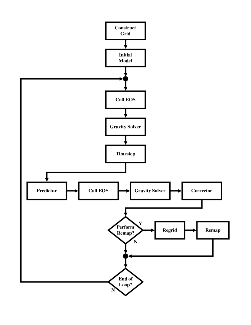
Figure 1.— The flowchart for BETHE-hydro. See §2 for a discussion.

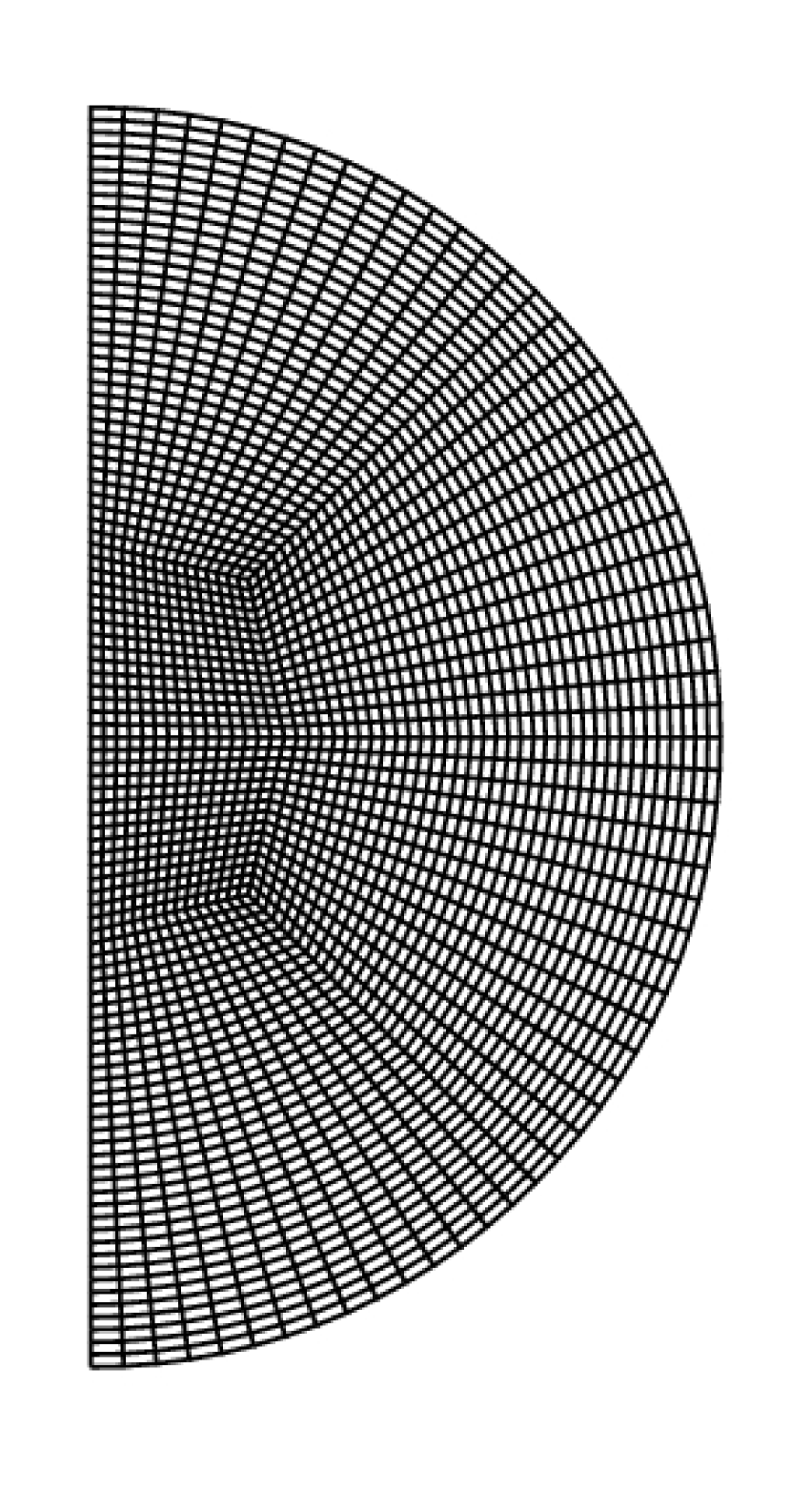
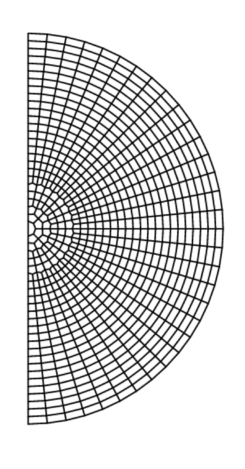
Figure 2.— On the left, a representative butterfly mesh and on the right, a representative spiderweb mesh. In general, we construct meshes with much higher resolution. However, to easily see the features of the mesh we reproduce low resolution versions here. The butterfly mesh is a standard grid that captures the benefits of a spherical grid near the outer boundary and avoids the singularity at the center. The spiderweb mesh captures the benefits of a spherical grid throughout, but near the center, the angular resolution is modified to avoid extreme Courant-condition limits and the singularity. Construction begins with half of an octagon at the center. Subsequent tiers of nodes are placed $\Delta r$ farther in radius from the interior set. When $r\Delta\theta$ exceeds $\Delta r$ the angular size is halved. For these transition nodes, $\Delta r$ is alternately multiplied by $1+\epsilon$ and $1-\epsilon$ to exaggerate the concavity of the cells.

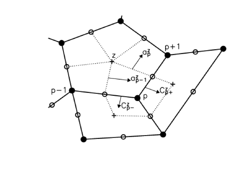
Figure 3.— A portion of an unstructured, polygonal mesh. Filled circles indicate node positions, $p$. Crosses mark cell centers, $z$. Open circles show the mid-edge locations. Cells are bounded by the edges (solid lines), and the cell is further divided into subcells via dashed lines. $\vec{C}^{z}_{p+}$ and $\vec{C}^{z}_{p-}$ are the half-edge area vectors. $\vec{a}^{z}_{p}$ and $\vec{a}^{z}_{p-1}$ are the area vectors for the lines connecting the cell centers and mid-edges (see §3 for a discussion).

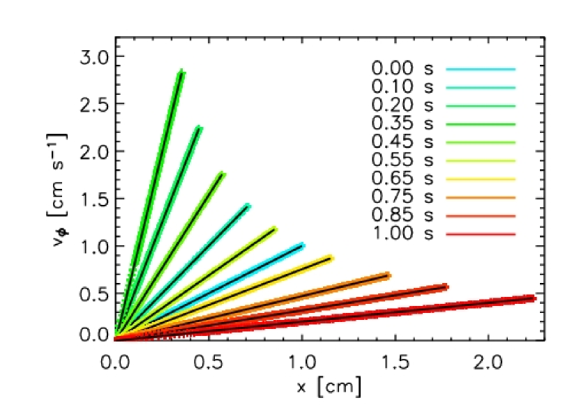
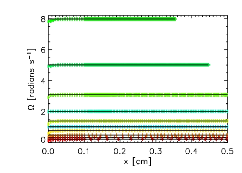
Figure 4.— Plots of $v_{\phi}$ vs. $r$ (top panel) and $\Omega$ vs. $r$ (bottom panel) for the simple rotational test discussed in §4.3.2. We employ three remapping regions. The inner 0.1 cm is Eulerian, zones exterior to 0.2 cm follow Lagrangian dynamics, and the region in between provides a smooth transition between the two domains. $v_{\phi}$ and $\Omega$ profiles are presented at $t=0.0,0.1,0.2,0.35,0.45,0.55,0.65,0.75,0.85$, and $1.0$ s. In the top panel, the deviation of the simulation (crosses) from the analytic solution (solid lines) is not discernible. The maximum error as measured by $(v_{\phi,{\rm ana}}-v_{\phi})/{\rm max}(v_{\phi,{\rm ana}})$ is $\sim 4\times 10^{-5}$ near the beginning of the simulation and $\sim 8\times 10^{-4}$ at the end. The $\Omega$ vs. $r$ panel (bottom) shows similar accuracy, except at the center, where $(\Omega_{\rm ana}-\Omega)$ reaches a maximum value of 0.2 rads s^-1 at $t=0.55$ s.

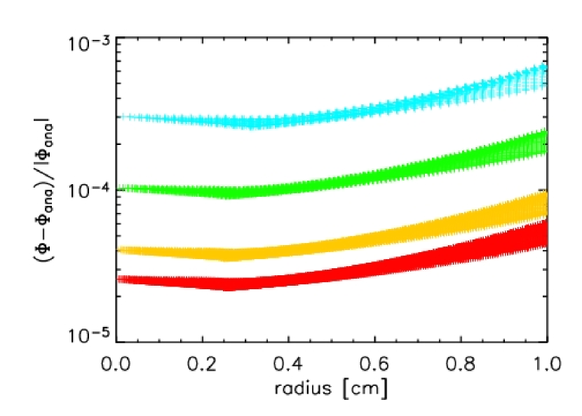
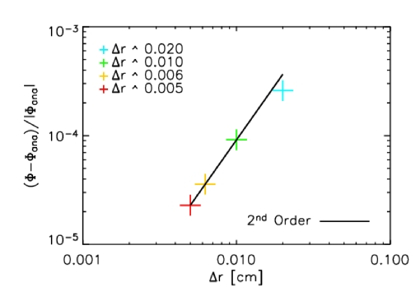
Figure 5.— Potential of a uniform density sphere. The density of the sphere is 1 g cm^-3 and the radius is 1 cm. Presented are results for four resolutions of the butterfly mesh (see left panel of Fig. 2): 2550 cells with an effective radial resolution $\Delta r\sim$ 0.02 cm (blue); 8750 cells with $\Delta r\sim$ 0.01 cm (green); 15,200 cells with $\Delta r\sim$ 0.006 cm (yellow); and 35,000 cells with $\Delta r\sim$ 0.005 cm (red). The top panel shows $(\Phi-\Phi_{\rm{ana}})/|\Phi_{\rm{ana}}|$, where $\Phi$ are the cell-center potentials as determined by the Poisson solver, and $\Phi_{\rm{ana}}$ is the analytic potential. The bottom panel shows the minimum error for each resolution as a function of the effective radial resolution. The solid line illustrates the fact that the 2D Poisson solver converges with 2^nd-order accuracy.

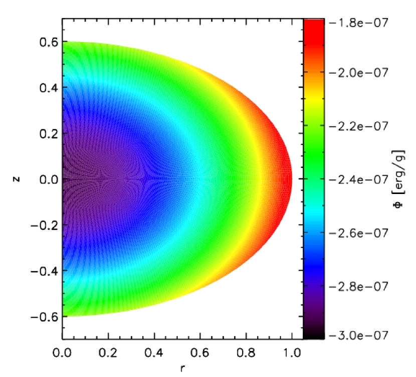
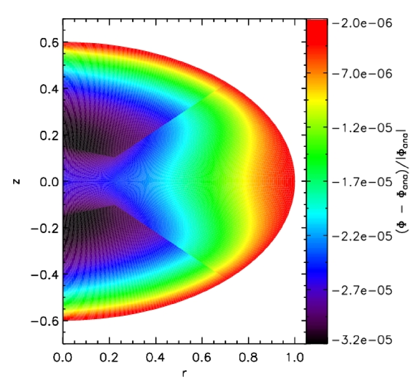
Figure 6.— The potential of a homogeneous spheroid with $e=0.8$ (top panel) and the relative accuracy of the potential, $(\Phi-\Phi_{\rm ana})/|\Phi_{\rm ana}|$ (bottom panel). $\rho_{0}=1$ g cm^-3 and the equatorial radius is $r_{a}=1$ cm. For the given eccentricity, the polar-axis radius, $r_{b}$, is 0.6 cm. The grid is a butterfly mesh, but the outer boundary follows the ellipse defining the surface of the spheroid. With $N_{\rm{cell}}=35,000$ and $\Delta r/r_{a}\sim 0.005$, the relative error in the potential ranges from $\sim$2 $\times 10^{-6}$ near the outer boundary to $\sim$3 $\times 10^{-5}$ in interior regions. Features in the relative error that track abrupt grid orientation changes in the mesh are apparent, but the magnitude of these features does not dominate the errors.

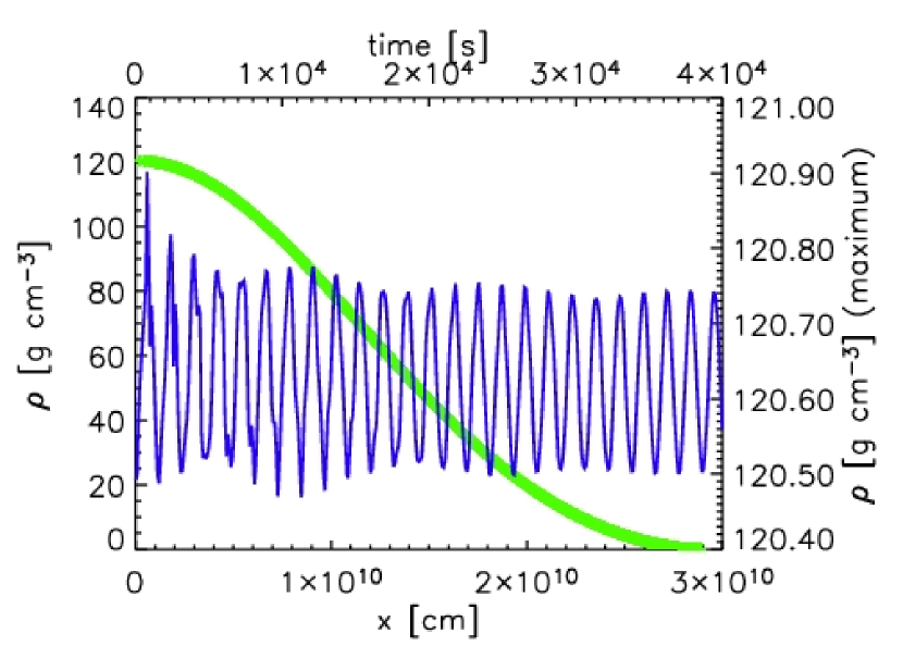
Figure 7.— Hydrostatic Equilibrium. The grid is the butterfly mesh with 8750 zones. The initial model is a Lane-Emden polytrope with $\gamma=5/3$, $M=1$ M_☉, and $R=2.9\times 10^{10}$ cm. The green crosses show the density profile at $t=1\times 10^{4}$ s. The solid line shows the maximum density as a function of time. The oscillations are due to the slight difference between an analytic hydrostatic equilibrium structure and a discretized hydrostatic equilibrium structure. This figure shows the code’s ability to follow oscillations for many periods with very little or no attenuation.

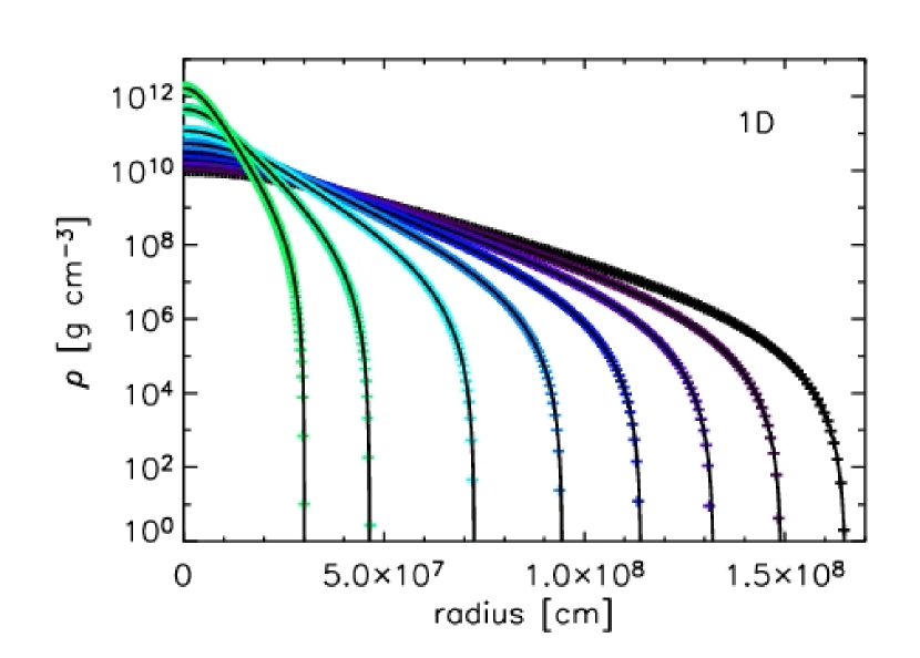
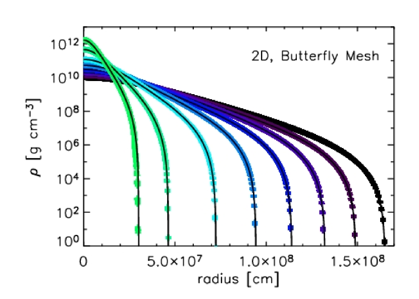
Figure 8.— Density profiles for Goldreich-Weber self-similar collapse in 1D (top panel) and 2D (bottom panel) and at $t=$0, 20, 40, 60, 80, 100, 120, and 130 ms. Simulation results (crosses) are compared with analytic solutions (solid lines). A gamma-law EOS is used with $\gamma=4/3$. The physical dimensions have been scaled so that $M=1.3$ M_☉, the initial central density is $10^{10}$ g cm^-3, and the maximum radius of the profile is $1.66\times 10^{8}$ cm. The initial grid for the 1D simulation uses 200 evenly-spaced zones. For the 2D simulation, a butterfly mesh with 35,000 zones with effectively 200 radial zones is used. These tests are calculated using the Lagrangian configuration. See §5.5 and Table 2 for quantitative discussion of the accuracy.

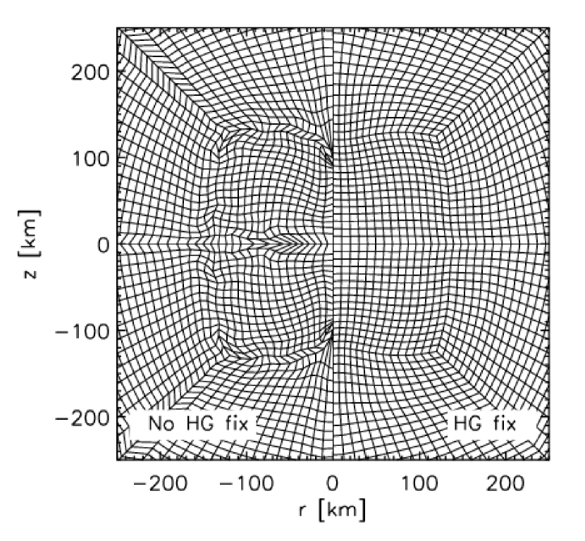
Figure 9.— Comparison when hourglass suppression is turned off (left) and on (right) for the Goldreich-Weber self-similar collapse. The simulations in this figure were run in the Lagrangian configuration with the butterfly mesh. Displayed in the region “$r>0$” are results at $t=0.118$ s when the hourglass suppression scheme of §8 is used and the scale factor has been set to 2.0. The results shown in the region “$r<0$” represent what happens when the hourglass suppression scheme is turned off.

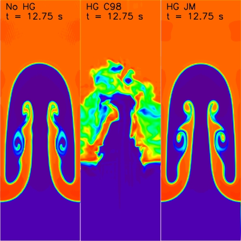
Figure 10.— Single-mode Rayleigh-Taylor instability: investigating hourglass suppression schemes (see §10.7 for a description of the setup). We present the results of the single-mode Rayleigh-Taylor instability with no hourglass fix (left panel), the hourglass subcell pressure scheme of Caramana & Shashkov (1998) (center panel), and the modified subpressure scheme described in this paper (right panel). While the results of the left panel are acceptable, there are hints of hourglass patterns in the contours. The central panel is a consequence of the incompatible nature of the subcell remapping scheme and the subcell pressure scheme of Caramana & Shashkov (1998), and our modified subpressure scheme (right panel) suppresses the hourglass distortions, while preserving the expected flow.

Figure 11.— Remapping a 1D step function. A step function in density is remapped many times with a grid that oscillates for two full cycles. There are 51 nodes (50 cells) and $n_{\rm max}=800$ remapping steps. The top panel displays the density profile for remapping steps 0 to $1/2n_{rmmax}$, and the bottom panel shows the profile for steps $1/2n_{\rm max}$ to $n_{\rm max}$. Initially, the discontinuity spreads over a small number of zones ($\sim$4), and in later steps (bottom panel) the discontinuity spreads very slowly.

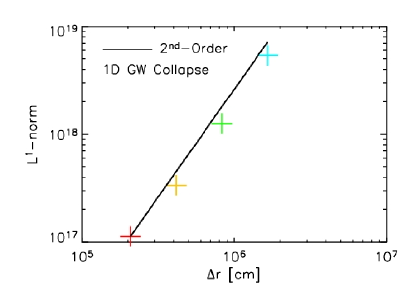
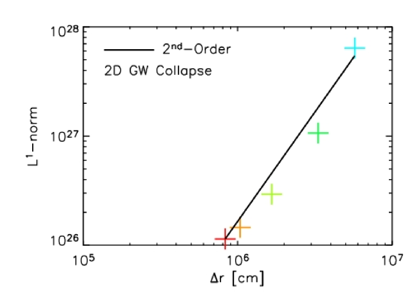
Figure 12.— The $L^{1}$-norm as a function of $\Delta r$ (crosses), the initial zone size, is plotted for Goldreich-Weber simulations in 1D (top panel) and 2D (bottom panel). The $L^{1}$-norm is calculated at t = 130 ms for both simulations. Both 1D and 2D simulations (crosses) converge with roughly 2^nd-order accuracy (solid line). See §10.1.

Figure 13.— Sod shock tube test. For a gamma-law EOS and $\gamma=1.4$, we compare the results of the 1D Lagrangian (bottom), 1D Eulerian (2nd from the bottom), 2D Lagrangian (3rd), and 2D Eulerian (top) Sod shock tube tests with the analytic result (solid lines). Other than the 1D Lagrangian results, the density profiles have been shifted vertically to distinguish features. The profiles are further separated by displaying them at different times: 1D Lagrangian ($t=0.2$ s), 1D Eulerian ($t=0.225$ s), 2D Lagrangian ($t=0.25$ s), and 2D Eulerian ($t=0.275$ s). The 1D calculations are resolved with 400 zones, and the 2D tests are resolved with 400x10 zones. See §10.2 for a discussion.

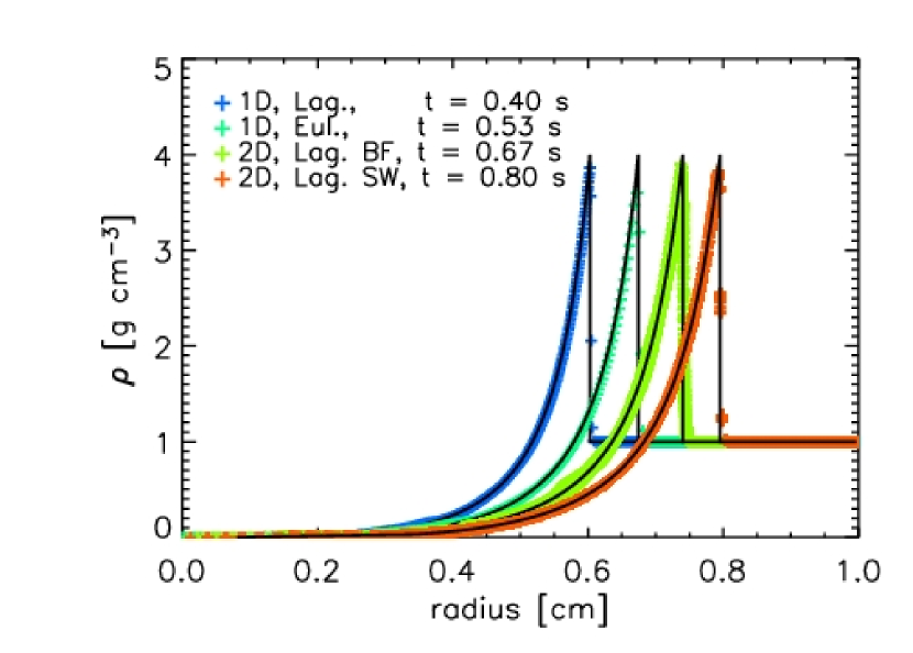
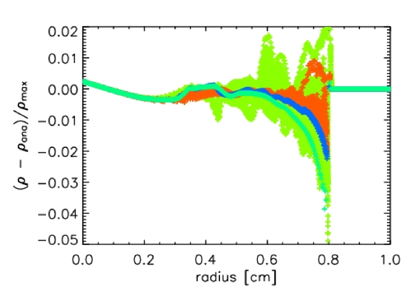
Figure 14.— Density profiles of the Sedov blast wave test. The Sedov blast energy is 0.244816 ergs. Initial conditions are $\rho_{0}=1.0$ g cm^-3, $\varepsilon_{0}=1\times 10^{-20}$ ergs g^-1, and the gamma-law EOS has $\gamma=5/3$. Top panel compares the simulations (crosses) with the analytic result (solid lines) for 1D Lagrangian ($t=0.4$ s), 1D Eulerian ($t=0.53$ s), 2D Lagrangian using the butterfly mesh ($t=0.66$ s), and 2D Lagrangian using the spiderweb mesh ($t=0.80$ s). 1D calculations are resolved with 400 zones. The spiderweb test has a total of 12,381 zones with 200 radial zones and a maximum of 64 angular zones. The butterfly mesh has a total of 35,000 zones with effectively 200 radial and 200 angular zones. Plotted in the bottom panel are the relative errors of the density, $(\rho-\rho_{\rm ana})/\rho_{\rm max}$, vs. radius, where $\rho$ is the simulated density profile, $\rho_{\rm ana}$ is the analytic profile, and $\rho_{\rm max}$ is the maximum density of the analytic profile.

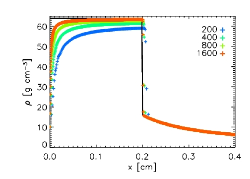
Figure 15.— Density profile for the Noh Problem at $t=0.2$ s. The solid line is the analytic solution for $\gamma=5/3$, and the crosses show the numerical results for resolutions of 200, 400, 800, and 1600 zones. The downturn of the density profile near the center is “wall heating,” a common problem for Lagrangian schemes (Rider, 2000). For the post shock material, the higher resolution runs capture the analytic solution. The upstream flow matches the analytic solution for all resolutions.

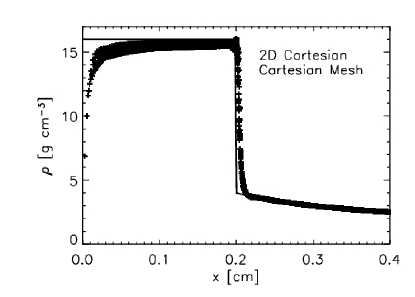
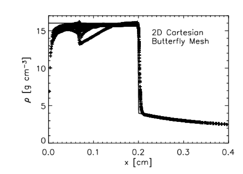
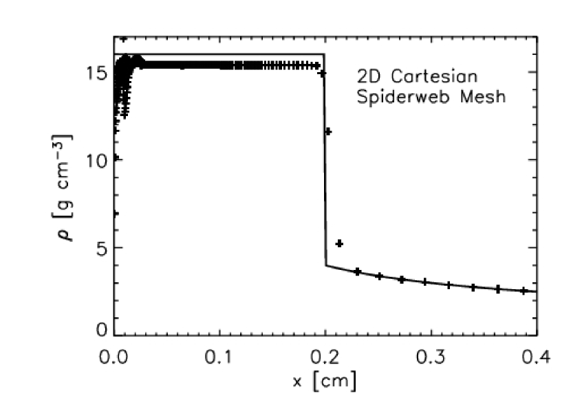
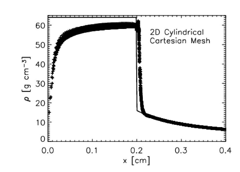
Figure 16.— Similar to Fig. 15, except here we present the results of 2D tests. All but the lower-right show results using 2D Cartesian coordinates. The lower-right shows results using 2D cylindrical coordinates. The grids used are: a Cartesian grid with 100$\times$200 zones (top-left and lower-right), a butterfly mesh with 22,400 zones (top-right), and a spiderweb mesh with 8550 zones (lower-left). Both the top-left and bottom-right panels indicate that using the Cartesian mesh produces fairly smooth results, with some ($\sim$7%) asymmetry in the post-shock region. Using the spiderweb mesh produces perfectly symmetric solutions except near the center where the deviation from symmetry is as large as $\sim$25%. Using the butterfly mesh produces similar mixed accuracy in symmetry.

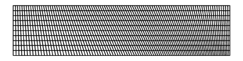
Figure 17.— Saltzman piston problem. This problem tests the code’s ability to resolve shocks that are oblique to the orientation of the grid. The top panel shows the initial grid with $100\times 10$ zones. The left wall is a piston moving at a constant velocity, 1.0 cm s^-1, to the right. Initially, the density and internal energy are set equal to 1.0 g cm^-3 and 0.0 ergs, respectively, and we use a gamma-law EOS with $\gamma=5/3$. The grid and the density colormap are shown in the bottom panel at $t=0.925$ s. See §10.5 for a discussion of the results.

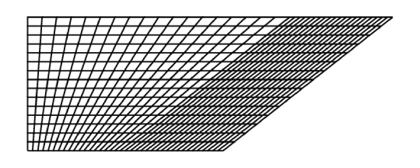
Figure 18.— The Dukowicz piston problem, another test using an oblique mesh. The initial setup involves two regions having an interface with a 60^∘ orientation with the vertical. The top panel shows a low-resolution example of the grid used. Region 1 has a density of 1 g cm^-3 and is resolved with $144\times 120$ zones, and region 2 has a density of 1.5 g cm^-3 and is gridded with a $160\times 120$ mesh, with the vertical mesh lines uniformly slanted at 60^∘. Initially both regions are in equilibrium with $P=1.0$ erg cm^-3. The left boundary is a piston with a velocity in the positive $x$ direction and a magnitude of 1.48 cm s^-1. The piston-driven shock travels from left to right, and encounters the interface. The incident shock continues to the lower density region, a transmitted/refracted shock propagates into the higher density region, a vortex sheet develops behind the transmitted shock, and a reflected shock propagates into the incident shock’s post-shock flow. The orientations of the flow are reproduced accurately (see §10.6 and Table 3).

Figure 19.— Nonlinear phase of a single mode of the Rayleigh-Taylor instability at $t=12.75$ s. The top and bottom densities are $\rho_{1}=2.0$ g cm^-3 and $\rho_{2}=1.0$ g cm^-3, respectively, and the gravitational acceleration points downward with magnitude $g=0.1$ cm s^-2. The top and bottom boundaries are reflecting while the left and right boundaries are periodic. From left to right, grid sizes are $50\times 150$, $74\times 222$, $100\times 300$ (this is the resolution used in Fig. 10), and $150\times 450$. See §10.7 for discussions comparing these results with those in other works.

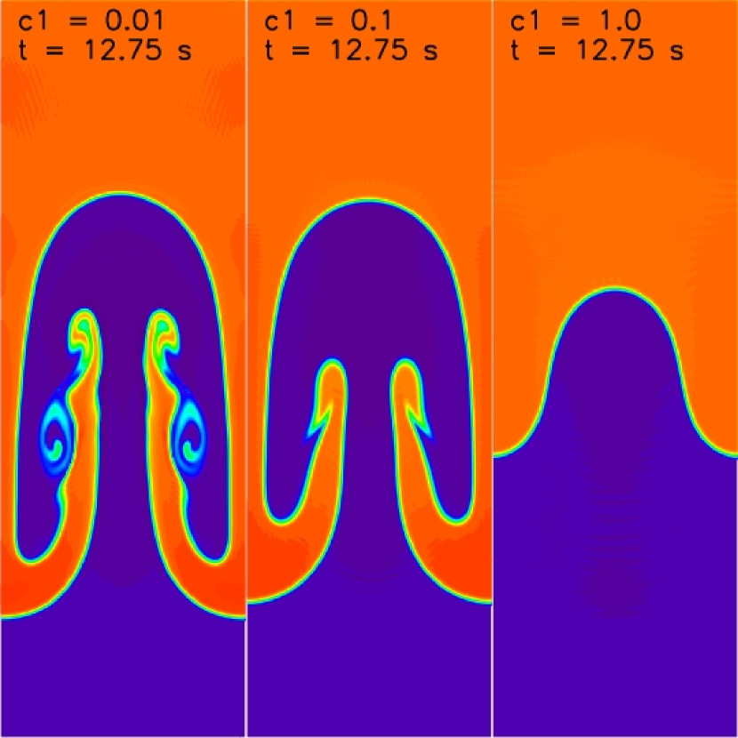
Figure 20.— Single-mode Rayleigh-Taylor instability: investigating the artificial viscosity parameter. The same resolution, setup, and time are shown as presented in Fig. 10 and the third panel of Fig. 19. Each panel shows results for different values of the artificial viscosity parameter, $c_{1}$, that is the coefficient of $c_{s}(\vec{\nabla}\cdot\vec{v})$ (see §7). The artificial viscosity parameters are $c_{1}=0.01$ (left panel), $c_{1}=0.1$ (center panel) and, $c_{1}=1.0$ (right panel). From this analysis, it would seem that one should choose the lower values of $c_{1}$ to accurately represent low Mach number Rayleigh-Taylor flows. However, higher values help to eliminate unwanted ringing in post shock flows.

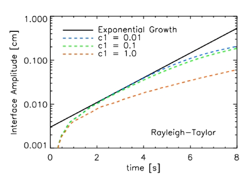
Figure 21.— The interface amplitude vs. time for the single-mode Rayleigh-Taylor instability test. Resolutions and setup are similar to those presented in Fig. 20. We compare the analytic exponential growth rate (solid line) with simulation results (dashed lines) for viscosity parameters, $c_{1}$, of 0.01, 0.1, and 1.0. Simulations with $c_{1}=0.01$ and 0.1 manifest exponential growth for several e-folding times, while the run with $c_{1}=1.0$ seems to follow the linear phase for only 1 s ($\sim$ 1/2 e-folding).

Figure 22.— Kelvin-Helmholtz shear instability. The domain is resolved with $256\times 256$ zones. The bottom region has $\rho_{\rm b}=1.0$, and the top region has $\rho_{\rm t}=\rho_{\rm b}/\chi$, where $\chi=8$, and both regions have $P=1.0$ erg cm^-3. A gamma-law EOS is used with $\gamma=5/3$. The top panel shows the development of Kelvin-Helmholtz rolls at $t=5.5$ s for $v_{\rm shear}=\frac{1}{4}c_{b}$ and $\tau_{\rm KH}$ 0.523 s. The bottom plot of Fig. 22 shows the interface amplitude (solid line) vs. time and compares to the expected exponential growth (dashed line) for a simulation with $v_{\rm shear}=\frac{1}{4}c_{b}$ (green) and $v_{\rm shear}=\frac{1}{2}c_{b}$ (blue). There are three distinct phases in the log-linear plot: an early transient phase, a phase in which the slope most closely matches the exponential growth rate, and the subsequent nonlinear phase.

Figure 23.— Density vs. radius for the core collapse of a 15-M_☉ star. The model is the s15 model of Weaver & Woosley. Density vs. radius for 1D (lines) and 2D (crosses) at times 0, 70, 110, 130, 140, and 150 ms after the start of the calculation. Core bounce occurs at 148 ms. The 2D grid is composed of a butterfly mesh in the interior with a minimum cell size of $\sim$0.5 km and extends to 50 km. A spherical grid extends the domain out to 4000 km. There are 23,750 cells in total, with an effective resolution of $\sim$250 radial and $\sim$100 angular zones. The 1D grid has 250 zones, with similar resolution to the 2D run at all radii. For the most part, the 1D and 2D calculations track one another quite well. There is roughly a $\sim$10% difference in the shock radii at 150 ms.

Figure 24.— Radial component of the gravitational acceleration during the core collapse of a 15-M_☉ star. Similar to Fig. 23. Note the good match between the 1D and 2D results.

Figure 25.— Angular velocity evolution during the core collapse of a rotating 15-M_☉ star. This test problem was calculated on the same grid as in Fig. 23. The initial angular velocity profile is constant on cylinders and is given by $\Omega(r)=1/(1+(r/A)^{2})$, where $A=1000$ km and $\Omega_{0}=2$ radians s^-1. As expected, the central angular velocity, $\Omega_{c}$ is proportional to $\rho_{c}^{2/3}$, where $\rho_{c}$ is the central density. The central density compresses from $\sim$10¹⁰ g cm^-3 at $t=0$ ms to $\sim$2.2 $\times 10^{14}$ g cm^-3 at $t=160$ ms. Therefore, at $t=160$ ms, $\Omega_{c}$ should be $\sim$1600 radians s^-1, consistent with results shown in this figure. Other than a slight, but noticeable, glitch at the location of the shock ($\sim$180 km), the angular velocity evolves smoothly with no evidence of axis effects.

References

- Agertz et al. (2007) Agertz, O., Moore, B., Stadel, J., Potter, D., Miniati, F., Read, J., Mayer, L., Gawryszczak, A., Kravtsov, A., Nordlund, Å., Pearce, F., Quilis, V., Rudd, D., Springel, V., Stone, J., Tasker, E., Teyssier, R., Wadsley, J., & Walder, R. 2007, MNRAS, 380, 963
- Barth (1997) Barth, T. J. 1997, Numerical Methods for Gasdynamic Systems on Unstructured Meshes, ed. T. Kroner, M. Ohlberger, & C. Rohde (Springer, Berlin), 195–285
- Bazán et al. (2003) Bazán, G., Dearborn, D. S. P., Dossa, D. D., Eggleton, P. P., Taylor, A., Castor, J. I., Murray, S., Cook, K. H., Eltgroth, P. G., Cavallo, R. M., Turcotte, S., Keller, S. C., & Pudliner, B. S. 2003, in Astronomical Society of the Pacific Conference Series, Vol. 293, 3D Stellar Evolution, ed. S. Turcotte, S. C. Keller, & R. M. Cavallo, 1–58381
- Bethe & Wilson (1985) Bethe, H. A., & Wilson, J. R. 1985, ApJ, 295, 14
- Buras et al. (2003) Buras, R., Rampp, M., Janka, H.-T., & Kifonidis, K. 2003, Physical Review Letters, 90, 241101
- Buras et al. (2006) —. 2006, A&A, 447, 1049
- Burrows et al. (2007a) Burrows, A., Dessart, L., Livne, E., Ott, C. D., & Murphy, J. 2007a, ApJ, 664, 416
- Burrows et al. (1995) Burrows, A., Hayes, J., & Fryxell, B. A. 1995, ApJ, 450, 830
- Burrows et al. (2006) Burrows, A., Livne, E., Dessart, L., Ott, C. D., & Murphy, J. 2006, ApJ, 640, 878
- Burrows et al. (2007b) —. 2007b, ApJ, 655, 416
- Campbell & Shashkov (2001) Campbell, J. C., & Shashkov, M. J. 2001, Journal of Computational Physics, 172, 739
- Caramana et al. (1998) Caramana, E. J., Burton, D. E., Shashkov, M. J., & Whalen, P. P. 1998, Journal of Computational Physics, 146, 227
- Caramana & Shashkov (1998) Caramana, E. J., & Shashkov, M. J. 1998, Journal of Computational Physics, 142, 521
- Chandrasekhar (1969) Chandrasekhar, S. 1969, Ellipsoidal Figures of Equilibrium (New Haven: Yale University Press)
- Colella & Woodward (1984) Colella, P., & Woodward, P. R. 1984, Journal of Computational Physics, 54, 174
- Dearborn et al. (2006) Dearborn, D. S. P., Lattanzio, J. C., & Eggleton, P. P. 2006, ApJ, 639, 405
- Dearborn et al. (2005) Dearborn, D. S. P., Wilson, J. R., & Mathews, G. J. 2005, ApJ, 630, 309
- Dukowicz & Meltz (1992) Dukowicz, J. K., & Meltz, B. 1992, Journal of Computational Physics, 99, 115
- Fryer & Warren (2002) Fryer, C. L., & Warren, M. S. 2002, ApJ, 574, L65
- Gardiner & Stone (2005) Gardiner, T. A., & Stone, J. M. 2005, Journal of Computational Physics, 205, 509
- Goldreich & Weber (1980) Goldreich, P., & Weber, S. V. 1980, ApJ, 238, 991
- Herant et al. (1994) Herant, M., Benz, W., Hix, W. R., Fryer, C. L., & Colgate, S. A. 1994, ApJ, 435, 339
- Hubeny & Burrows (2007) Hubeny, I., & Burrows, A. 2007, ApJ, 659, 1458
- Janka & Mueller (1995) Janka, H.-T., & Mueller, E. 1995, ApJ, 448, L109
- Kitaura et al. (2006) Kitaura, F. S., Janka, H.-T., & Hillebrandt, W. 2006, A&A, 450, 345
- Klein (1999) Klein, R. I. 1999, J. Comp. App. Math, 109, 123
- Kucharik et al. (2003) Kucharik, M., Shaskov, M. J., & Wendroff, B. 2003, Journal of Computational Physics, 188, 462
- Landshoff (1955) Landshoff, R. 1955, A Numerical Method for Treating Fluid Flow in the Presence of Shocks, Tech. rep., Los Alamos National Laboratory
- LeBlanc & Wilson (1970) LeBlanc, J. M., & Wilson, J. R. 1970, ApJ, 161, 541
- Liebendörfer et al. (2001a) Liebendörfer, M., Mezzacappa, A., & Thielemann, F.-K. 2001a, Phys. Rev. D, 63, 104003
- Liebendörfer et al. (2001b) Liebendörfer, M., Mezzacappa, A., Thielemann, F.-K., Messer, O. E., Hix, W. R., & Bruenn, S. W. 2001b, Phys. Rev. D, 63, 103004
- Liebendörfer et al. (2006) Liebendörfer, M., Pen, U.-L., & Thompson, C. 2006, in International Symposium on Nuclear Astrophysics - Nuclei in the Cosmos
- Liebendörfer et al. (2005) Liebendörfer, M., Rampp, M., Janka, H.-T., & Mezzacappa, A. 2005, ApJ, 620, 840
- Liska & Wendroff (2003) Liska, R., & Wendroff, B. 2003, SIAM J. Sci. Comput., 25, 995
- Livio et al. (1980) Livio, M., Buchler, J. R., & Colgate, S. A. 1980, ApJ, 238, L139
- Livne (1993) Livne, E. 1993, ApJ, 412, 634
- Livne et al. (2004) Livne, E., Burrows, A., Walder, R., Lichtenstadt, I., & Thompson, T. A. 2004, ApJ, 609, 277
- Loubère & Shashkov (2005) Loubère, R., & Shashkov, M. J. 2005, Journal of Computational Physics, 209, 105
- Loubère et al. (2006) Loubère, R., Staley, M., & Wendroff, B. 2006, Journal of Computational Physics, 211, 385
- Margolin (1988) Margolin, L. G. 1988, A centered artificial viscosity for cells with large aspect ratio, Tech. rep., Lawrence Livermore National Laboratory
- Margolin & Shaskov (2003) Margolin, L. G., & Shaskov, M. J. 2003, Journal of Computational Physics, 184, 266
- Margolin & Shaskov (2004) —. 2004, Computer Methods in Applied Mechanics and Engineering, 193, 4139
- Miller et al. (1993) Miller, D. S., Wilson, J. R., & Mayle, R. W. 1993, ApJ, 415, 278
- Miniati & Colella (2007) Miniati, F., & Colella, P. 2007, Journal of Computational Physics, 227, 400
- Monaghan (1992) Monaghan, J. J. 1992, Annu. Rev. Astron. Astrophys., 30, 543
- Morel et al. (1998) Morel, J. E., Roberts, R. M., & J., S. M. 1998, Journal of Computational Physics, 144, 17
- Müller & Steinmetz (1995) Müller, E., & Steinmetz, M. 1995, Computer Physics Communications, 89, 45
- Rampp & Janka (2002) Rampp, M., & Janka, H.-T. 2002, A&A, 396, 361
- Rider (2000) Rider, W. J. 2000, Journal of Computational Physics, 162, 395
- Ruge & Stuben (1987) Ruge, J. W., & Stuben, K. 1987, Algebraic multigrid (AMG), ed. S. F. S. F. McCormick (Philadelphia, PA: SIAM), 73â130
- Shashkov & Steinberg (1995) Shashkov, M. J., & Steinberg, S. 1995, Journal of Computational Physics, 118, 131
- Shashkov & Steinberg (1996) —. 1996, Journal of Computational Physics, 129, 393
- Shen et al. (1998) Shen, H., Toki, H., Oyamatsu, K., & Sumiyoshi, K. 1998, Nuclear Physics A, 637, 435
- Smarr et al. (1981) Smarr, L., Wilson, J. R., Barton, R. T., & Bowers, R. L. 1981, ApJ, 246, 515
- Stone & Norman (1992) Stone, J. M., & Norman, M. L. 1992, ApJS, 80, 753
- Symbalisty (1984) Symbalisty, E. M. D. 1984, ApJ, 285, 729
- Thompson et al. (2003) Thompson, T. A., Burrows, A., & Pinto, P. A. 2003, ApJ, 592, 434
- Truelove et al. (1998) Truelove, J. K., Klein, R. I., McKee, C. F., Holliman, II, J. H., Howell, L. H., Greenough, J. A., & Woods, D. T. 1998, ApJ, 495, 821
- Von Neumann & Richtmyer (1950) Von Neumann, J., & Richtmyer, R. D. 1950, J. Appl. Phys., 21, 232
- Wilkins (1980) Wilkins, M. L. 1980, J. Comput. Phys., 36, 281
- Woodward & Colella (1984) Woodward, P., & Colella, P. 1984, Journal of Computational Physics, 54, 115
- Woosley & Weaver (1995) Woosley, S. E., & Weaver, T. A. 1995, ApJS, 101, 181