Mechanical Systems that are both Classical and Quantum

Abstract

Quantum dynamics can be regarded as a generalization of classical finite-state dynamics. This is a familiar viewpoint for workers in quantum computation, which encompasses classical computation as a special case. Here this viewpoint is extended to mechanics, where classical dynamics has traditionally been viewed as a macroscopic approximation of quantum behavior, not as a special case.

When a classical dynamics is recast as a special case of quantum dynamics, the quantum description can be interpreted classically. For example, sometimes extra information is added to the classical state in order to construct the quantum description. This extra information is then eliminated by representing it in a superposition as if it were unknown information about a classical statistical ensemble. This usage of superposition leads to the appearance of Fermions in the quantum description of classical lattice-gas dynamics and turns continuous-space descriptions of finite-state systems into illustrations of classical sampling theory.

A direct mapping of classical systems onto quantum systems also allows us to determine the minimum possible energy scale for a classical dynamics, based on a localized rate of state change. We use a partitioning description of dynamics to define locality, and discuss the ideal energy of two model systems.

1 Introduction

A digital photograph looks continuous but in fact, if you examine it closely enough, you discover that there is only a finite amount of detail. Similarly, a digital movie looks like it is changing continuously in time, but in fact it is actually a discrete sequence of digital images.

Something similar is true of nature. Although the world looks to our senses as if it has an infinite amount of resolution in both space and time, in fact a finite-sized physical system with a finite energy has only a finite amount of distinguishable detail and this detail changes at only a finite rate [27].

1.1 A bit of history

The finite character of the states of physical systems came as a great surprise when it became apparent at the start of the twentieth century. The revolution was started by Max Planck in 1900 when he found that he had to introduce a new constant into physics in order to understand the thermodynamics of electromagnetic radiation in a cavity. The new constant fixed the statistical mechanical analysis, but it did so by making the count of distinct possible states finite.

Planck’s constant has a particularly simple interpretation in classical statistical mechanics. There, the number of microscopic ways a system can realize a macroscopic state is taken to be proportional to the volume in phase space (i.e., position/momentum space) of states consistent with the parameters that define the macroscopic state. In units where Planck’s constant is one, the phase space volume becomes the actual finite count of distinct states. Planck’s constant is the fundamental grain size in phase space, representing one state.

Although Planck’s constant was initially introduced to fix statistical mechanics, a new dynamical theory also grew from this beginning. The resulting quantum mechanics established new rules for describing the microscopic dynamics of physical systems. The QM rules were, of course, constructed so that the well established rules of classical mechanics would be recovered as a limiting case. The continuous equations of motion in CM correspond to the limit in which Planck’s “fundamental grain size in phase space” goes to zero. In this limit, a finite-sized physical system has an infinite number of distinguishable states and passes through an infinite subset of these states in a finite amount of time. Even though an actual finite-sized physical system has only a finite number of distinct states and a finite rate of state change, if these finite numbers are large enough (as they would normally be in a macroscopic system) the motion is well approximated by the continuous CM equations.

1.2 Classical finite-state models

The finite-state and finite-rate character of physical systems make classical finite state models of fundamental interest in physics. This is because classical models are easier to understand and simulate than quantum models.

In statistical mechanics, classical finite-state lattice systems have a long history as models of phase change phenomena in magnetic materials and mixtures of fluids [22, 18, 41, 8]. Such classical lattice gases can be considered special cases of general quantum lattice systems and described and analyzed using the same quantum formalism [33]. By looking at these special cases, we gain insight into macroscopic classical concepts such as entropy and phase change by seeing them arise from underlying classical finite-state systems.

We might hope to similarly gain insight by studying classical special cases of quantum dynamics. Any such classical special case must (like any other finite physical system) necessarily have only a finite number of distinct states.

The most common classical finite-state models of physical dynamics are numerical approximations of continuum models. These are not good candidates to be special cases of microscopic physical dynamics, though, because in this case it is the theoretical continuum model that has realistic physical characteristics, not its truncated and rounded-off finite-state realization [39]. The best candidates for exact special cases are lattice dynamics generalizations of classical lattice gases. These are lattice models with exact finite-state conservation laws, that at large scales can exhibit not only realistic thermodynamic behavior but also realistic classical mechanical behavior such as wave propagation and fluid dynamics [32, 28]. These models have been used to simulate physical dynamics [25] but have not previously been studied as classical special cases of quantum dynamics.

1.3 Finite-state physical dynamics

Any invertible classical logic operation can be implemented as a QM unitary dynamics, and so can any composition of such operations. Since there are additional operations needed to implement an arbitrary QM unitary dynamics [1], classical finite-state dynamics is logically a proper subset of quantum dynamics.

Before the advent of invertible models of computation [4, 12] and QM models of computation [3, 24, 5] it wasn’t obvious that, from a logical standpoint, a classical dynamics could be regarded as a special case of quantum dynamics. Historically, the viewpoint had been that classical dynamics is a purely macroscopic concept, relevant only in a limit in which quantum effects become negligible. In retrospect the confusion stems from not considering the possibility of invertible classical finite-state dynamics—an understandable omission since QM was developed before computer ideas were prevalent, let alone the idea of invertible computation!

We are glossing over a significant issue, though, when we picture classical finite-state dynamics as a composition of unitary operations. In a quantum computer [1, 5], the structures that switch from one unitary operation to the next are assumed to be macroscopic and classical. Thus it seems that our picture is incomplete since there are unspecified things going on to implement the explicitly time-dependent sequence of unitary operations. It is helpful to note, though, that if we take the limit of an infinitely large array of finite-state elements going through a simple cycle of unitary operations, we can recover the familiar time-independent equations of continuum QM [6, 19, 30, 9, 43]. Thus explicit time dependence at the microscopic scale does not preclude compositions of unitary operations from being equivalent to more traditional time-independent models of physical dynamics.

Even if there is nothing essential missing from explicitly time-dependent QM models, it’s not clear that they embody what we’re looking for here: a classical-quantum correspondence that is so direct that we might hope to interpret the quantities and concepts of quantum dynamics in a simpler classical context. If we have to traverse a continuum limit in order to make contact with the familiar time-independent quantities and concepts of continuous dynamics, we lose this directness.

1.4 Continuous dynamics

Much of the simplicity of QM derives from the use of continuous operators. For example, if two QM operators $A$ and $B$ obey a commutation relationship of the form $[A,B]=c$ for $c$ a non-zero constant, then the operators $A$ and $B$ must necessarily be infinite-dimensional. For this reason the fundamental operators describing position and momentum in QM are continuous, just as they are in CM.

When a (finite-state) physical system is described as a quantum system in continuous space, specifying the state of the system for a finite number of points in space completely determines the future evolution. This suggests that we may be able to construct continuous CM models that are special cases of continuous QM dynamics if they also have this property.

A famous example of a CM system of this sort is Fredkin’s billard ball model of computation (BBM)[12]. This is an embedding of finite-state reversible computation into continuous CM. At integer times, all billiard balls are found at integer coordinates in the plane, all moving at the same speed in one of four directions. Collisions between billiard balls perform conditional logic—where a ball ends up after a collision depends on whether or not another ball was present to collide with it.

1.5 Finitary classical mechanics

A finite-sized BBM system is an example of what we might call a finitary CM dynamics: one for which exact future states can be computed indefinitely using a finite number of logical operations.

Finitary CM systems are special cases of CM that are equivalent to a finite state dynamics when observed only at integer times. In such systems the motion remains perfectly continuous between integer times, but dynamical parameters (masses, spring constants, etc.) are chosen carefully and all dynamics is assumed to be perfect so that, as long as the initial state is chosen from a finite set of allowed states, one of the same allowed set is seen at each integer time (we only consider synchronous systems here, cf. [24]).

Since constraints are placed only on the values of dynamical parameters and the initial values of state variables, finitary CM systems map all of the continuous Lagrangian machinery and conservations of CM onto finite-state dynamics. At integer times the system is equivalent to a finite-state lattice dynamics such as a lattice gas automaton or partitioning automaton [32, 28]. From a continuum perspective, though, state variables arrive at integer coordinates in space at integer times—they don’t remain on a fixed lattice at intermediate times. This is a subtle but important distinction. The same distinction in QM models allows infinite-dimensional position and momentum operators to be applied to particles that are always found at integer coordinates in continuous space at integer times.

1.6 Outline of the paper

The remainder of this paper is divided into four sections.

Section 2: Quantum concepts in a classical context discusses simple examples of recasting a classical finite-state dynamics as a continuous finitary CM dynamics and thence as a continuous quantum dynamics. The quantum description is closely related to classical sampling theory. Fermions and Bosons appear in the quantum description of classically identical particles.

Section 3: Ideal energy uses the correspondence between QM and finitary CM to define an ideal energy for finitary CM dynamics. This is the minimum total energy that is compatible with the rate of local state change. A partitioning description of dynamics defines local state change.

Section 4: An elastic string model and Section 5: A colliding ball model define and analyze finite-state partitioning models that can be embedded in a continuous relativistic dynamics. We discuss the relationship between ideal energy and relativistic kinetic energy in these models.

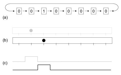
Figure 1: Embedding a finite-state classical dynamics. (a) Shift register with a single 1. (b) Classical particle in a box. (c) Quantum particle in a box.

2 Quantum concepts
in a classical context

To illustrate some issues involved in describing CM dynamics using QM, and how QM concepts look in this classical context, we discuss in this section the simplest examples: non-interacting particle models. These models are embeddings of an $N$ bit shift register. We start with the case where all bits of the shift register are 0’s except for a single 1 (Figure 1a). At each discrete time step the register is circularly shifted one position to the right: the 1 hops to the next position to the right, and if it is in the rightmost position it hops to the first position.

2.1 Classical particle in a box

The discrete-shift dynamics can be embedded into a continuous shift (Figure 1b). We replace the register with a one-dimensional space, and the 1 by a free particle moving to the right at a constant speed $s$. The space is periodic, so that when the particle exits at one end, it reappears at the other end. If the length of the space is $L$, then we take our unit of distance to be $L/N$ and our unit of time to be $L/Ns$. The particle is started at an integer coordinate, moving to the right at speed $s$. It will subsequently always be found at one of the $N$ integer coordinates at any integer time. Interpreting the presence or absence of a particle at a position as a 1 or a 0, the continuous system reproduces the discrete-shift dynamics at integer times.

Conversely, the time evolution of the continuous system can be exactly predicted at integer times by evolving the discrete-shift system. This implies that the continuous system, with a finite set of allowed integer-time states, effectively has no more distinct states than the finite-state system. From the point of view of the discrete-shift dynamics intermediate states are fictitious states that have been added in order to construct a continuous embedding.

In this example, as in the other finitary CM examples we will consider, the finite subset of the continuous state set that can be visited by the dynamics at integer times is known when the system is defined and doesn’t change with time. Periodic discreteness makes the details of the fictitious states between integer times irrelevant for predicting the long-term behavior of the dynamics.

2.2 Particle in a quantum box

Given finite energy a QM particle in a box can be completely described using only a finite set of distinct states. One could regard the CM embedding of the shift register example above as a semiclassical analog of a QM particle in a box, illustrating how a system with a dynamics that obeys a continuous translational symmetry can be made to act like a finite state system by restricting the set of allowed initial states in a manner that is conserved at integer times by the dynamics.

We can make this more than an analogy by recasting the continuous CM “particle in a box” dynamics in QM language.

2.2.1 Unidirectional Hamiltonian

Consider a free massless relativistic particle in a one dimensional periodic box. If we ignore for a moment that the particle can travel both left and right we can take the Hamiltonian to be $H=cp$, where $p=-i\hbar\partial/\partial x$ is the usual momentum operator and $c$ is the speed of light. The Schrödinger equation becomes

$$i\hbar{\partial\psi\over\partial t}=H\psi=-ci\hbar{\partial\psi\over\partial x}$$ (1)

This has the solution $\psi(x,t)=f(x-ct)$, where $f(x)$ is the initial state of $\psi$ at $t=0$ and can be specified arbitrarily. This dynamics just shifts whatever state we start with uniformly to the right at speed $c$.

Now we assume that this system has finite energy. In QM, this assumption imposes constraints on the allowed initial states. The conventional way to analyze this for a QM particle in a box is to describe the particle’s position in terms of momentum eigenstates: only waves that fit an integer number of wavelengths across the width of the box are allowed by the boundary conditions. Since momentum eigenstates with higher spatial frequencies correspond to higher energies, a finite maximum energy eigenstate only allows us to use a finite number of frequency components.

2.2.2 Energy based counting of states

The QM average energy corresponds to the classical energy, and so the natural constraint for a closed classical dynamical system is that the average energy is bounded (rather than the maximum energy eigenvalue). We will take the average energy constraint as the starting point for the analysis in this section.

Average energy is related to rate of state change [27]: for any closed QM system, the average energy $E$ (taking the ground state energy as zero) gives an achievable bound on the rate $\nu_{\perp}$ at which the system can pass through a long sequence of distinct (i.e., mutually orthogonal) states:

$$\nu_{\perp}\leq 2E/h$$ (2)

Now suppose the particle is initially very well localized. Then the initial wavefunction $f(x)$ is sharply peaked at one point and zero everywhere else. Under the “shift” dynamics, after a short time the sharp peak will have moved enough so that the old and new position states will be distinct (Figure 1c). The more sharply the particle is localized, the sooner the states will be distinct and so the higher the rate of orthogonal change and hence the higher the average energy. If instead the “peak” is spread evenly over the whole box, the shift will never produce a different state and the average energy can be very low.

Given a finite average energy $E$ there is thus a limit to how sharply the particle can be localized and this determines how many distinct position states are available to the system. If the width of the box is $L$ and there are $N$ distinct position states, then the system transitions to a new orthogonal state in the time it takes the pattern to shift a distance of $L/N$. Thus the rate at which the system passes through orthogonal states is $\nu_{\perp}=cN/L$ and so, from Equation 2, $N$ can’t be more than $2LE/ch$. The maximum number of distinct states is bounded by the energy $E$. Since the average (classical) momentum is $E/c$, this can also be written as $N\leq 2pL/h$.

2.2.3 Bidirectional Hamiltonian

The unidirectional Hamiltonian we’ve used here seems unphysical, since a real particle should be able to move in either direction. The direction should be part of the state, not part of the Hamiltonian. This can easily be fixed. Since the Hamiltonian $H=cp$ moves the particle uniformly to the right at speed $c$ without changing the shape of the wavefunction, clearly the Hamiltonian $H=-cp$ would carry the particle uniformly to the left at speed $c$. If we make a two component state vector and use the Hamiltonian

$$H=\left(\begin{array}[]{cc}cp&0\\ 0&-cp\end{array}\right)$$ (3)

then the particle will travel to the right if we represent it in the first component, and to the left if we represent it in the second component. If we define

$$\sigma=\left(\begin{array}[]{cc}1&0\\ 0&-1\end{array}\right)$$ (4)

then the Hamiltonian can be written as $H=c\,\sigma p$. Thus $\sigma$ can be interpreted as the operator that reads the sign of the particle direction from the state information. This is a one-dimensional version of the Weyl equation, sometimes also referred to as the massless Dirac equation.

$$\begin{array}[]{c@{\hspace{.6in}}c}\includegraphics[height=108.405pt]{Figures/ss-gg-comparison}\hfil\hskip 43.36243pt&\includegraphics[height=108.405pt]{Figures/pulse-real-imag}\\ \mbox{\bf(a)}\hfil\hskip 43.36243pt&\mbox{\bf(b)}\\ \end{array}$$

Figure 2: Cardinal Sine Probability Distribution. (a) Normalized sinc² distribution function (solid) versus normalized Gaussian of the same height (dotted). (b) Real (solid) and imaginary (dotted) components of sinc-based amplitude distribution.

2.3 Discrete position basis

In Figure 1c, we depicted the wavepacket representing the particle as a square wave. In this section we discuss the actual shape of the wavepacket needed to achieve the energy bound of Section 2.2.2 on the number of distinct states.

If we were just specifying a discrete distribution at integer times and positions, the probabilities needed to reproduce the shift dynamics are obvious: the particle is at some integer position with probability 1 and at other integer positions with probability 0. We want to extend this distribution to the continuum.

For continuous positions, the width of the wavepacket represents uncertainty in where exactly the particle would be found if we looked. Since the shape of the wavepacket doesn’t change as it shifts, we are free to interpret all of the uncertainty as uncertainty in the initial position of the particle.

There is, however, a better way to interpret this. The shape of the wavepacket is chosen to allow us to represent exactly $N$ distinct states, each with the wavepacket centered at an integer coordinate. The uncertainty in particle position blurs distinctions, combining continuum states that would otherwise be distinct. Thus another way to interpret the position uncertainty would be to say that we invented fictitious intermediate positions in order to map a finite-state dynamics onto the continuum, and then we treated the exact value of the position coordinate as if it was uncertain in order to eliminate the fictitious position information by representing it probabilistically as missing information.

Now, if we represented the particle by a square pulse, as in Figure 1c, we would be assigning equal probabilities to all fictitious intermediate positions in one region and zero elsewhere, with a sharp transition in between. The only constraint on the continuous wavefunction, however, is that it should exactly represent the finite-state dynamics when sampled at integer times and positions. We should therefore choose the wavefunction that includes as little information as possible about fictitious intermediate positions (i.e., in keeping with Jaynes Maximum Entropy Principle [17], we should choose the wavefunction that is maximally noncommital with regard to missing information). This implies a bound on the Fourier spectrum of the wavefunction: spatial frequencies that are needed only to specify details about fictitious intermediate positions should be omitted.

In Figure 2a we illustrate a probability distribution function based on the cardinal sine function,

$${\mbox{\rm sinc}}\>x={\sin x\over x}$$ (5)

Cardinal sine gets its name as the basis of E. T. Whittaker’s cardinal interpolation function, and it plays a central role in bandlimited sampling theory [35, 31]. It is the Fourier transform of a finite range of frequency components, all taken with equal weight. The probability distribution function shown with the solid line is ${\mbox{\rm sinc${}^{2}$}}{\pi u}$. This is a normalized distribution that is close to a Gaussian (dotted line) near the mean, has the value 1 at the point $u=0$ and has the value 0 at every other integer position.

The corresponding amplitude distribution for a particle centered at integer position $m$ is ${\mbox{\rm sinc}}\>{\pi(u-m)}$ times a phase factor. Of course this function also has magnitude one at the center of the distribution, and magnitude zero at all other integer positions. We can use a weighted sum of such functions to construct any assignment of amplitudes to integer positions. Figure 2b shows the real and imaginary parts of the function

$$\phi(\pi u)=e^{i\pi u}\>{\mbox{\rm sinc}}\>{\pi u}$$ (6)

The set of functions $\phi(\pi(u-m))$ for $m$ an integer are all mutually orthogonal: these functions form a complete basis. We will refer to these states as the discrete position basis.

The discrete position basis states (and any states constructed out of them) have a bounded spatial frequency spectrum. These basis states answer the question we started this section with: for the shift dynamics, they have the waveshape that achieves the maximum possible rate of orthogonal change for a given average energy (Equation 2). The average energy of a particle in a discrete position basis state is $h/2\tau$, where $\tau$ is the time it takes the particle to travel from one integer position to the next. We derive these fastest-changing states directly from the Hamiltonian $H=c\,p$ in the next section.

2.4 Bandlimited dynamics

A general construction for fastest changing states is given in [27]. These states are essentially Fourier transforms of a finite set of energy eigenstates, which are the slowest changing states.

In the macroscopic limit, the discrete position basis states of Equation 6 are fastest changing states (for given average energy) of a 1D particle evolving under the shift dynamics. The case we are interested in, however, is finite and periodic. It is instructive to construct the exact states that achieve the energy bound of Equation 2 in this case. If we consider a situation where the particle travels only to the right (Equation 1), then the energy eigenstates satisfy the equation

$$-ci\hbar{\partial\psi\over\partial x}=E\psi$$ (7)

We assume that our energy scale is chosen so that the smallest value of $E$ is zero. This equation is satisfied by an exponential of $x$. If we use positive $x$ coordinates that range from 0 to $L$ in the box, then the generic solution that is periodic at $x=L$ is given by $\psi_{n}\propto e^{2\pi inx/L}$, where $n$ is a non-negative integer. This function satisfies Equation 7 provided

$$E=nh{c\over L}$$ (8)

In our CM embedding of an $N$-bit shift register dynamics, the only meaningful positions at integer times are $x_{u}=u\,L/N$ for $u$ an integer: the wavefunction at the (fictitious) non-integer positions is a continuous extension, completely determined by the values at the integer positions. Thus we require that the probabilities of finding the particle at integer positions at integer times add up to one, and so

$$\psi_{n}(x_{u})={1\over\sqrt{N}}e^{2\pi inu/N}$$ (9)

for which $\sum_{u}\psi_{n}^{*}(x_{u})\psi_{n}(x_{u})=1$. Using Equations 8 and 9 we can construct a normalized fastest changing state centered at position zero: in this case it is simply the sum of the $N$ different $\psi_{n}$’s taken with equal amplitudes [27]. Therefore the fastest changing state centered at position $x_{m}$ is given by

$$\Phi_{m}(x_{u}) = {1\over\sqrt{N}}\sum_{n=0}^{N-1}\psi_{n}(x_{u}-x_{m})$$ (10)

$$= {1\over N}\sum_{n=0}^{N-1}e^{2\pi in(u-m)/N}$$ (11)

$$= {\sin{\pi(u-m)}\over N\sin{\pi({u-m\over N})}}e^{i\pi(u-m)(1-{1\over N})}$$ (12)

where the final expression comes from summing the geometric series and some rearrangement. The fastest changing states are Fourier transforms of the energy eigenstates. For large $N$, $\Phi_{m}(x_{u})$ turns into $\phi(\pi(u-m))$ of Equation 6. $\Phi_{m}(x_{u})$ also has the property that it is one for $u\equiv m\allowbreak\mkern 10.0mu({\operator@font mod}\,\,N)$ and zero for $u$ any other integer. For integer values of $u$, the $\Phi_{m}(x_{u})$ functions provide a complete discrete-position basis for the finite system.

2.5 Both continuous and discrete

The discrete position basis state $\Phi_{m}(x_{u})$ corresponds to a probability distribution that is normalized both from a continuous and a discrete point of view. Furthermore, the discrete normalization doesn’t apply just to a sampling of the state at integer locations: it applies to any discrete sampling of the state at a unit-spaced set of positions.

The continuous normalization is apparent from Equation 11, since

$$\displaystyle\int_{0}^{L}dx\;\Phi_{0}^{*}(x)\,\Phi_{0}(x)$$ (13)

$$= {1\over N^{2}}\sum_{n=0}^{N-1}\sum_{n^{\prime}=0}^{N-1}\int_{0}^{N}du\;e^{2\pi iu(n^{\prime}-n)/N}$$

$$= 1$$

To see the generality of the discrete normalization, we similarly sum over positions $x_{u+\delta}$ where $u$ is an integer and $0<\delta<1$. This shifted normalization also implies that if we start the system in a discrete-position basis state, then as the wavefunction shifts continuously with time the values sampled at fixed integer locations always constitute a normalized discrete representation of the state.

Both normalization properties are of course inherited by any normalized wavefunction $\Psi(x,t)$ constructed out of the $\Phi_{k}$ states (i.e., any $\Psi$ whose spectrum of spatial frequencies is bandlimited like the $\Phi$’s). $\Psi(x,t)$ can be exactly reconstructed from the amplitudes $\Psi(x_{k},t)$ sampled at integer locations:

$$\Psi(x,t)=\sum_{k=0}^{N-1}\Psi(x_{k},t)\,\Phi_{k}(x)$$ (14)

2.6 Intermediate positions

We can construct a $\Phi_{c}$ state centered at any continuum position $c$ as a superposition of the $N$ discrete-position basis states $\Phi_{m}$ centered at integer locations $m$. This is obvious since the $\Phi_{m}$ states form a complete basis for describing the continuously shifting time evolution of an initial $\Phi_{m}$ state. A shift of all $\Phi_{m}$ states by the same amount yields a new basis.

If we start our system with a particle at an integer location in a basis state and then change bases in step with the particle motion, we can follow the continuous motion of the particle, always seeing it in a single localized basis state. From this point of view the quantum motion is just as spatially local and continuous as the classical motion: in both cases we see the constraint on the classical system of a discrete set of possible positions at integer times reflected as a corresponding discrete set of possible intermediate positions at each intermediate time.

2.7 Classical Fermions and Bosons

The shift register example is easily extended to multiple particles. This simply corresponds to a value in the register (Figure 1a) with more than a single ‘1’ bit. For simplicity, we’ll assume for the moment that all particles are traveling to the right.

In elementary QM, the overall state of a collection of independent particles is normally represented using a product of single-particle states: we track the state of each particle separately as if it were the only particle in the system.

For our classical shift register we’ve already described a single particle system using a localized wavepacket basis (Equation 12). Here we’ll denote the single particle basis state where particle $j$ has its wavepacket centered at location $x$ as $\left|x,j\right\rangle$. An overall state can be described as a product of such states, one per particle.

Since all particles are moving to the right, the direction $\sigma$ is +1 in all cases. The Hamiltonian for a multi-particle system is then $H=\sum_{j}cp_{j}$, where $p_{j}$ acts only on particle $j$. For example, for a two particle system (i.e., shift register with two 1’s), the Schrödinger equation would be

$$i\hbar{\partial\mbox{$\left|x,0\right\rangle$}\mbox{$\left|y,1\right\rangle$}\over\partial t} = (cp_{0}+cp_{1})\mbox{$\left|x,0\right\rangle$}\mbox{$\left|y,1\right\rangle$}$$ (15)

$$= (cp_{0}\mbox{$\left|x,0\right\rangle$})(cp_{1}\mbox{$\left|y,1\right\rangle$})$$

This equation is satisfied if both $i\hbar{\partial\mbox{$\left|x,0\right\rangle$}/\partial t}=cp_{0}\mbox{$\left|x,0\right\rangle$}$ and $i\hbar{\partial\mbox{$\left|y,1\right\rangle$}/\partial t}=cp_{1}\mbox{$\left|y,1\right\rangle$}$ hold, and so the two particles each follow a shift dynamics.

By using a product of single-particle wavefunctions to construct our multiparticle wavefunction we’ve added two kinds of extra states that didn’t exist in the original shift register. First of all, our states can represent more than a single 1 at the same location, which isn’t possible in the original shift register. Secondly, our states keep track of which particle is which, but these particles are identical 1’s in a shift register and interchanging two 1’s in a binary number doesn’t give us a different state!

We can fix both of these problems by combining each set of equivalent states into a single state. We do this by adding together all product states that differ only by a relabeling of identical particles and we call that a single state. In performing this sum on a set of $M$ equivalent states we weight half of the states by a factor of $+1/\sqrt{M}$ and half by $-1/\sqrt{M}$. This is done in such a manner that the entire combination changes sign if we interchange any two particle labels (i.e., it is antisymmetrized). In our two particle example, the antisymmetrized wavefunction is

$$\psi={\mbox{$\left|x,0\right\rangle$}\mbox{$\left|y,1\right\rangle$}-\mbox{$\left|y,0\right\rangle$}\mbox{$\left|x,1\right\rangle$}\over\sqrt{2}}$$ (16)

Using only antisymmetrized wavefunctions we can no longer represent two particles (1’s) at the same location: as in this example, if two mean positions are equal (i.e., $x=y$) the wavefunction is zero.

Replacing each set of equivalent states with a single antisymmetrized sum avoids over-representing states. For a classical embedding into QM, a superposition of classically distinct states corresponds to a classical statistical ensemble: we can interpret all probabilities as arising from ignorance about which single state the system started in. Thus by assigning equal probabilities to a set of equivalent states, the antisymmetrized superposition represents the equivalent states as if we were completely ignorant about which particle was which. Of course the particle label information doesn’t exist in the original finite-state dynamics and so, once again, the probabilities we’ve assigned represent ignorance of fictitious classical details added in constructing our QM description.

Thus for a classical dynamics of bits, if a fixed number of identical 1’s are described quantum mechanically as if we could distinguish which is which, and then the fictitious distinctions are eliminated using superposition, they are Fermions. If, instead, there were no constraint in our original classical dynamics on how many 1’s can be represented at each location, we would use symmetrization rather than antisymmetrization to eliminate the fictitious distinctions. In this case the 1’s would be Bosons.

2.8 Non-classical amplitudes

There are two kinds of probabilities that can arise in a quantum description of a classical finite-state dynamics. There may be unknown information about the state of the actual dynamics: this is represented by ordinary probabilities and contributes to the entropy of the system. There may also, however, be unknown information about fictitious classical details that were added in constructing the quantum description of the dynamics (such as distinct labels for identical 1’s): this is represented by probabilities derived from amplitudes and doesn’t contribute to the entropy of the system.

There is more to amplitudes than this, though. If the dynamics was always described in a single classical basis, then the superposition would evolve like a classical statistical ensemble and the coefficient of a basis state in the superposition could be any function of the basis state’s ensemble probability—there is no recombining of coefficients in the ensemble dynamics. The fact that amplitudes are square roots of probabilities makes it possible to also use them to describe the system in multiple bases: the sum of the squares of component magnitudes is the same for a vector described in any basis. Amplitudes, when used for basis change, still don’t represent unknown information about the real system, and so again don’t contribute to its entropy.

2.9 Finite-state unitary dynamics

For a classical finite-state system with a conserved number of identical 1’s, we can treat the 1’s as distinguishable particles in a QM description and follow their trajectories. We can then use appropriate symmetrization of superpositions of products of single particle states to merge equivalent states that aren’t actually distinguishable.

We can extend this approach to describe classical systems in which the numbers of 1’s and 0’s are not constant. The creation (and annihilation) operators of quantum field theory allow us to act on an appropriately symmetrized superposition of products of single-particle states, to add (or remove) a single-particle basis state in each product term while maintaining the symmetrization of the overall state. We can use an occupation-number basis to avoid dealing directly with single-particle states, but a vestige of antisymmetrization persists as anticommutation of Fermionic field operators [44].

We can avoid all of this complexity entirely, though, by simply not describing identical 1’s as if they were distinguishable! We won’t have to nullify fictitious particle labels using symmetrization if we don’t put them in in the first place. Similarly, unnecessary complexity is added when we employ a continuum of positions and times to describe a classical system with only a finite number of possible states.

Both sources of complexity are eliminated if the QM dynamics is constructed to be isomorphic to the classical finite-state dynamics. If we start with a classical dynamics expressed as a composition of invertible logic operations we can, in the QM description, simply replace each classical logic operation with an equivalent finite-time finite-state unitary transformation. There are then no extra states added to the description that need to be nullified. Moreover, if the finite-state dynamics can be interpreted as an integer-time sampling of a finitary CM dynamics, then it is easy to identify the familiar continuous-space and -time conserved quantities of CM, including classical energy. The corresponding identification of QM energy is discussed in the next section.

3 Ideal energy

In CM there is no minimum energy required to allow a given sequence of state changes to take place in a given period of time. In QM, there is. If a classical finite-state dynamics is recast isomorphically as a unitary QM dynamics we can place a bound on the least possible average energy for physically realizing the classical dynamics—the ideal energy of the dynamics (cf. [24]).

For a dynamics described as a composition of spatially-localized invertible operations, Equation 2 allows us to define a minimum energy bound $E_{\mbox{\rm\scriptsize state-change}}$ that depends on counting state changes:

$$E_{\mbox{\rm\scriptsize state-change}}={h\over 2\tau}*(\mbox{state-changes in $\tau$})$$ (17)

Here $\tau$ is the length of the time interval during which we count state changes. Each invertible operation that actually changes the state counts as one state change.

Now, in CM, energy of motion appears as localized state change. Thus the state-change energy we define here can be thought of as a kind of kinetic energy: it bounds classical energy of motion, at a given time. The total classical energy is then bounded by the maximum value that the state-change energy acquires in the course of the time evolution.

In this section we discuss state-change energy and use it to define the ideal minimum energy of a finitary CM dynamics. In Sections 4 and 5 we apply this idea to two examples of finitary CM dynamics.

3.1 Classical partitioning dynamics

If a spatially extended finite-state system evolves in time synchronously, the rate of global state change dramatically underestimates the minimum energy needed for an actual physical realization of the dynamics. In particular, the energy of a collection of independent subsystems is additive: localized independent changes must be counted separately.

We can arrive at a more realistic minimum-energy estimate by making use of the locality and time dependence inherent in a physical description of classical finite state dynamics. Consider, for example, a finitary CM dynamics such as Fredkin’s BBM. In this model, all collisions happen synchronously, at a discrete set of possible locations at a discrete set of possible times. If we focus on a time interval starting shortly before a possible collision time and ending shortly after, then during this interval the system can be partitioned into a set of disjoint regions, each of which evolves independently: within each region one or more particles head towards the locus of a possible collision, collide or don’t collide, and then head away from the locus. Which regions evolve independently must of course change with time or the particles could never cross between regions. Thus the partitioning used in a description of the system as a collection of independent subsystems must be time dependent, even though the continuous dynamics itself follows a time independent dynamical law.

$$\begin{array}[]{c}\includegraphics[height=108.405pt]{Figures/swap7}\\ \end{array}$$

Figure 3: Integer-time history of two particles moving continuously in a periodic box.

Figure 3 illustrates the partitioning idea applied to the “classical particles in a periodic box” model discussed in Section 2. A time history from this finitary CM dynamics is shown, with the positions of two continuously moving particles (1’s) sampled at integer times. If the spatial intervals marked with solid lines in the figure are taken to be blocks of a partition, then during the period between one integer time and the next any particles that start off in a block remain in that block and only interact with other particles in the same block. The classical finite-state dynamics at integer times can be summarized as: swap the values (1’s or 0’s) at the two integer locations in each block of the partition.

Notice that, looking just at the integer-time history, it is ambiguous whether continuously moving particles whose paths intersect pass through each other or bounce back. This kind of ambiguity is very common in extending a finite-state dynamics to construct an equivalent finitary CM dynamics. If, however, we only want to quantify the minimum possible amount of motion consistent with a given classical finite-state dynamics, then there is no ambiguity. For example, for the dynamics illustrated in Figure 3, the least amount of motion occurs if the two particles don’t move between steps 2 and 3.

Of course in a real CM dynamics, the amount of motion that occurs inside the block where the two particles collide and bounce back could be small if they slow down quickly, but not exactly zero. We might think of zero motion either as a limit or, alternatively, as the exact amount of motion seen at the midpoint of the block update.

3.2 Ideal kinetic energy

The integer-time swap dynamics of Figure 3 can be described as a time-dependent sequence of unitary operations, with operations acting first on each block of one partition, and then on each block of the other partition.

Equation 17 assigns $h/2\tau$ of state-change energy to each block update involving a single moving particle. This agrees with our earlier QM analysis of the minimum achievable energy for a freely moving CM particle. Since there is no kinetic energy associated with blocks that don’t change, either in the CM or the QM description, the state-change energy defines an ideal kinetic energy in this case: it is at all times the minimum kinetic energy that could possibly be achieved in a physical realization of the dynamics. Its maximum value is the ideal total energy.

In general, the definition of kinetic energy in a finitary CM dynamics is somewhat ambiguous. For example, the same dynamics might be interpretable as either a relativistic system or a non-relativistic system [29]. If the state-change energy is taken as the ideal kinetic energy at all times, this ambiguity is resolved. Even if this is not done, however, the state-change energy sets the ideal energy scale, since it bounds the minimum total energy that can be involved in each possible block transition: for any CM interpretation of the dynamics one of these bounds will be the most constraining.

Below, we discuss ideal energy in two example models, beginning with a model that is closely related to the swap dynamics.

$$\begin{array}[]{c@{\hspace{.6in}}c@{\hspace{.6in}}c}\includegraphics[width=122.85876pt]{Figures/wave1}\hfil\hskip 43.36243pt&\includegraphics[width=122.85876pt]{Figures/wave2}\hfil\hskip 43.36243pt&\includegraphics[width=122.85876pt]{Figures/wave3}\\ \mbox{\bf(a)}\hfil\hskip 43.36243pt&\mbox{\bf(b)}\hfil\hskip 43.36243pt&\mbox{\bf(c)}\\ \end{array}$$

Figure 4: Discrete wave dynamics. Elastic string is held fixed where it crosses black bars.

4 An elastic string model

In this section we discuss a classical finite state model of wave motion in an elastic string. The finite-state string model corresponds exactly to the integer-time behavior of a continuous CM model of the type discussed in Section 1.5. The finite-state string model also exactly reproduces the behavior of the time-independent one-dimensional wave equation sampled at integer-times and locations. There is a finite-state constraint on the allowed initial shape and motion of each unit segment of the wave and this constraint reappears at each integer time. In the continuum limit the discrete constraint on the wave disappears; the exactness of the wave dynamics itself (at discrete times) is not dependent on this limit.

The model presented here has been discussed before [16, 28, 40], but the analysis of translational motion, the relativistic interpretation and the analysis of ideal-energy given here are all new.

4.1 Discrete wave model

Consider an ideal continuum string for which transverse displacements exactly obey the wave equation. In Figure 4a we’ve illustrated an initial configuration with this string stretched between equally spaced vertical bars. The set of initial configurations we’re allowing are periodic, so the two endpoints must be at the same height. Any configuration is allowed as long as each segment running between vertical bars is straight and lies at an angle of $45^{\circ}$.

Initially the string is attached at a fixed position wherever it crosses a vertical bar. We start the dynamics by releasing the attachment constraint at all of the gray bars. The attachment to the black bars remains fixed. In Figure 4b the segments that are about to move are shown with dotted lines: the straight segments have no tendency to move. Under continuum wave dynamics, the dotted segments all invert after some time interval $\tau$. This will be our unit of time for the discrete dynamics. The new configuration at the end of this interval is shown in Figure 4c. At this instant in time all points of the string are again at rest and we are again in an allowed initial configuration. At this instant we interchange the roles of the black and gray bars and allow the segments between adjacent gray bars to move for a time inteval $\tau$. The dynamics proceeds like this, interchanging the roles of the black and gray bars after each interval of length $\tau$. Since attachments are always changed at instants when all energy is potential and the string is not moving, the explicit time dependence of the system doesn’t affect energy conservation.

$$\begin{array}[]{c@{\hspace{.6in}}c@{\hspace{.6in}}c}\includegraphics[height=108.405pt]{Figures/waves-rule-a}\hfil\hskip 43.36243pt&\includegraphics[height=108.405pt]{Figures/waves-rule-b}\hfil\hskip 43.36243pt&\includegraphics[height=108.405pt]{Figures/waves-rule-c}\\ \mbox{\bf(a)}\hfil\hskip 43.36243pt&\mbox{\bf(b)}\hfil\hskip 43.36243pt&\mbox{\bf(c)}\\ \end{array}$$

Figure 5: Discrete wave dynamics. (a) Wave configuration with possible wave paths indicated (dotted lines). (b) One of two partitions used for a discrete update rule (horizontal and vertical lines). Array of wave gradients shown at bottom. (c) Top, dynamical rule for wave. Presence of wave-path segments is indicated by 1’s. Bottom, equivalent dynamical rule for gradients.

We express this dynamics as a purely digital rule in Figure 5. In Figure 5a we show the wave just after the evolution from the previous figure, with the black bars shown marking the attachments for the next step. To simplify the figure we have suppressed the gray bars—they are always situated midway between the black bars and so don’t need to be shown. We have also added a grid of $45^{\circ}$ dotted lines that shows all of the segments that the string could possibly follow. In Figure 5b we add in horizontal black bars, in order to partition the 2D grid into a set of 2$\times$2 blocks that can be updated independently. Note that in all cases the segments that are allowed to change during this update step, as well as the cells that they will occupy after the update, are enclosed in a single block. Segments that aren’t going to change stretch across multiple blocks. The 1D box below Figure 5b contains just the slope information from the string. This array of gradients is clearly sufficient to recreate the wave pattern if the height at one position is known.

Figure 5c shows the dynamical rule for a block. Since the dotted lines indicate the direction in which segments must run if they appear in any cell, the state information for each segment is only whether it is there or not: this is indicated with a 0 or a 1. The only segments that change are peaks /\ or valleys \/, and these are represented by two 1’s at the top of a block or at the bottom of a block respectively. The rule is that peaks and valleys turn into each other, and nothing else changes. This rule applies to the blocking shown, and then to the complementary blocking when the attachments change, alternating back and forth. This is a partitioning dynamics.

$$\begin{array}[]{c@{\hspace{.8in}}c@{\hspace{.8in}}c}\includegraphics[height=101.17755pt]{Figures/short-wave}\hfil\hskip 57.81621pt&\includegraphics[height=101.17755pt]{Figures/long-wave}\hfil\hskip 57.81621pt&\includegraphics[width=86.72377pt]{Figures/continuous-wave}\\ \mbox{\bf(a)}\hfil\hskip 57.81621pt&\mbox{\bf(b)}\hfil\hskip 57.81621pt&\mbox{\bf(c)}\\ \end{array}$$

Figure 6: Rescaling a discrete wave. (a) Original wave and array listing its gradients. (b) Each pair of gradients is repeated four times. The corresponding wave is drawn by placing gradients end-to-end. (c) Equivalent superposition of continuous waves.

4.2 Exact wave behavior

At the bottom of Figure 5c we’ve presented a dynamics for the gradient of the wave. Since the full 2D dynamics just turns peaks into valleys and vice versa, leaving straight segments unchanged, we can perform that dynamics equally well on the array of gradients! As the 2D dynamics interchanges which blocking to use, the dynamics on the gradients also alternates which pairs of gradients to update together. In all cases, the dynamics on the gradients duplicates what happens on the string: if the two dynamics are both performed in parallel, the gradient listed below a column will always match the slope of the string in that column.

The dynamics on the gradients has a very interesting property. Turning a peak into a valley and vice versa is exactly the same as swapping the left and right elements of a block. Leaving a // or \\ unchanged is also exactly the same as swapping the left and right elements of a block. In all cases, the dynamics on the gradients is equivalent to a swap.

This means that the left element of a block will get swapped into the right position, and at the next update it will be the left element of a new block and will get swapped into the right position, and so on. Thus all of the gradients that start off in the left side of a block will travel uniformly to the right, and all of the gradients that start in the right side of a block will travel uniformly to the left.

This shows that the system obeys a discrete version of the wave equation. Half of the gradients constitute a right-going wave, and half constitute a left-going wave. At any step of the dynamics, the 2D wave in the original dynamics is just the sum of the two waves: it is reproduced by laying gradients end to end!

As the number of cells in our lattice gets arbitrarily large, the straight segments in our waves become smaller and smaller compared to the total width of the lattice, and the discrete wave equation turns smoothly into exactly the continuum wave equation. As we will see, though, even the discrete model exactly obeys the continuum wave equation.

4.3 Rescaling limit

The discrete wave system also has another continuum limit that allows us to embed our discrete wave dynamics with time-dependent blocking into a continuous dynamics with a time-independent dynamical law.

Take an array of gradients that define a wave (Figure 6a) and make a longer list by replicating every pair of segments $N$ times, producing a list that is $N$ times as long (Figure 6b). Since the dynamics for the gradients is simply that all of the even numbered gradients shift one way and all of the odd numbered gradients shift the other, the state after $N$ steps corresponds exactly to the state we would have gotten by running one step on the original configuration, pairing the gradients into the alternate set of blocks and then replicating each block $N$ times.

Although the $N$-step dynamics is exactly equivalent to the original, the waves we reconstruct from the array of repeated blocks look much different than simply a scaled up version of the original wave: a peak /\ doesn’t turn into a peak $N$ times as large, it turns into $N$ little peaks /\/\/\.../\. This is a wiggly flat line, and as $N$ grows the wiggles get proportionately smaller and smaller compared to the straight parts // and \\, which simply get $N$ times longer. In the limit, the peaks turn into flat places with a net velocity up or down, still obeying the continuum wave equation.

4.4 Continuous at all scales

The rescaled continuum configurations correspond isomorphically with the discrete time evolution, since a flat portion of the wave moving up or down can simply be interpreted as an array of peaks or valleys. In fact, if we simply draw each block of the active partition that we’ve been showing as /\ or \/ as a horizontal segment moving up or down instead, then the discrete dynamics is directly mapped onto the continuous wave equation without invoking any limiting process!

Since this evolution obeys the continuous wave equation we can draw it as the superposition of continuous rightgoing and leftgoing waves. This is shown in Figure 6c. The top solid wave is a redrawing of Figure 6a with a horizontal segment used instead of the /\ (or equivalently, the continuum limit of Figure 6b). It is also the sum of the dotted rightgoing and leftgoing waves shown below it, each segment of which has slope $\pm 1/2$. The collection of gradients that make up the rightgoing and leftgoing waves are shown at the bottom. These are just the even position (top) and odd position (bottom) gradients from Figure 6a, each stretched to fill the width of a block. After the waves each move half the width of a gradient segment, all segments will again be aligned and will add up to a result that corresponds to the next step of the discrete wave dynamics, with the appropriate blocking.

4.5 Relativistic motion

Assume the string carrying a discrete wave wraps around a space of width $N$. We’ve discussed the horizontal motion of waves along such a string, but the string itself can move vertically. For example, a pattern such as /\/\/\.../\ all the way around the space reproduces itself after two steps, but shifted vertically by two lattice units. This is clearly the maximum rate of travel for a string: one position vertically per time step.

We can express the net velocity of the string in terms of the populations of rightgoing and leftgoing gradient segments. With $N$ positions there are $N/2$ rightgoing segments and $N/2$ leftgoing segments, and the members of each group never change. Thus if there are $R$ rightgoing \’s, there must be $(N/2)-R$ rightgoing /’s, and similarly for the other direction. Therefore if we know the numbers $R$ and $L$ of rightgoing and leftgoing \’s, we have complete population information.

For a wave that wraps around the space and joins at the ends, there must be equal numbers of /’s and \’s. Thus half of the gradient segments must be \’s,

$$R+L={N\over 2}$$ (18)

The average upward velocity of the string depends on the difference between $R$ and $L$,

$${R-L\over N/2}=v$$ (19)

If we think of the dynamics as swapping adjacent pairs of gradients during each step (even though \\ and // pairs don’t actually change), each gradient moves one position up or one position down during each update. A \ moving right always moves the gradient it passes one up as it goes by, whereas a \ moving left moves the gradient it passes one down. Thus we get Equation 19 for the average velocity of gradients that pass the $N/2$ \’s. The average velocity of gradients that pass the /’s is exactly the same (their populations are complementary but the effects of passing them are also complementary).

Since the motion of each gradient contributes a velocity of $\pm 1$ to the the net motion of the string, it is natural to interpret the net motion relativistically. We can focus on just the \ particles, since the / particles have the same behavior. The total energy is proportional to the number of identical particles all moving at the same speed, so we let $E=R+L=N/2$ (Equation 18). Since $P=Ev$ (taking $c=1$), this gives us a vertical momentum of $P=R-L$ (Equation 19). Then the mass of the string must be $M^{2}=E^{2}-P^{2}=4RL$ and $E=\gamma M$ where $\gamma=(1-v^{2})^{-1/2}$.

We can exactly analyze the vertical motion of the string statistically, since the probability $p=R/(R+L)$ is the exact frequency with which leftgoing gradients will encounter a rightgoing \ in the course of a cycle of length $N/2$.

A rightgoing gradient is the left element of a block of two adjacent string segments that are about to be updated by the dynamical rule. If the block contains \/ then the dynamics will move both elements upward one position. Thus $p$ is the probability that, for any block holding part of the string, the left element of the string is ready to take an upward step, and $1-p$ the probability it is ready to take a downward step.

Similarly, if a block contains \ as its right element (i.e., a leftgoing \), then the block is ready to take a downward step if the left element is /. The chance that the block contains a leftgoing \ is $L/(R+L)$ which is just $1-p$. Thus in either position of a block, $p$ is the probability a gradient is ready to take an upward step and $1-p$ the probability it is ready to take a downward step, and so the average frequency (per step) of both elements of a block moving upward is $p^{2}$ and both downward is $(1-p)^{2}$. The average upward velocity of the string is thus $p^{2}-(1-p)^{2}$ which just gives us back Equation 19.

4.6 Relativistic kinetic energy

Our original continuous description of the elastic string dynamics involved minimal-motion between integer times: all cases remain motionless except for \/ and /\, which turn into each other. Thus the least possible energy for this transition determines the ideal kinetic energy for the string dynamics.

Since the average frequency (per step) of both elements of a block moving upward is $p^{2}$ and both downward is $(1-p)^{2}$, the average fraction of the blocks that change per step is $p^{2}+(1-p)^{2}$. This fraction times $N/2$, the total number of blocks in the string, gives (using Equation 17) the least possible average kinetic energy (in energy units of $h/2\tau$). Since the motion exactly repeats after a cycle of $N/2$ steps, the ideal kinetic energy per cycle is invariant.

The minimum value of $p^{2}+(1-p)^{2}$ is $1/2$ and occurs when $p=1/2$, which is also when $v=0$. Thus at low speeds, half of the block changes don’t contribute to the net vertical motion of the string. If we think of the string as a particle moving in one dimension (i.e., vertically) with a horizontal internal dimension of width $N$, then only the portion of the ideal kinetic energy that contributes to vertical motion is particle kinetic energy. Thus at low speeds, the ideal particle kinetic energy is the excess over $1/2$ of the blocks that change,

$$T_{\mbox{\rm\scriptsize non-rel}} = {N\over 2}\left(p^{2}+(1-p)^{2}-{1\over 2}\right)$$ (20)

$$= E\left(\left({1+v\over 2}\right)^{2}+\left({1-v\over 2}\right)^{2}-{1\over 2}\right)$$

$$= {1\over 2}Ev^{2}$$

Since $E=\gamma m$, for small $v$ we have $E=m$ and we recover the expected non-relativistic kinetic energy.

As $p$ approaches zero or one, the fraction of the blocks that change approaches one and the vertical speed of the string also approaches one. Thus as $v\to 1$, all of the ideal kinetic energy contributes to the string motion: $T\to E$.

4.7 Time dilation

If we think of the block changes that don’t contribute to overall string motion as internal dynamics of the string, then as the string approaches the speed 1 the internal dynamics stops: all of the changes contribute to overall string motion and none to internal dynamics. The internal dynamics exhibits relativistic time dilation. There is a slight subtlety, though, that arises from relativistically interpreting all gradient segments as moving. We correspondingly interpret a fraction $1/\gamma$ of all segment motion as contributing to the internal motion, and so the internal dynamics slows down by this factor as the string speeds up. The remaining fraction $1-1/\gamma$ of the segment motion contributes to the overall string motion. Of course some of the internal “motion” we’re counting here doesn’t involve block changes, but all of the segment motion that contribute to overall motion of the string does actually correspond to block changes. Thus the fraction of all $N/2$ blocks of the string that contribute to kinetic energy of string-particle motion is in fact $1-1/\gamma$ (i.e., $T=E-m$). The fraction of blocks that contribute only to internal kinetic energy in the string is then the total fraction that change minus the external kinetic fraction, and so

$$T_{\mbox{\rm\scriptsize internal}} = {N\over 2}\left(p^{2}+(1-p)^{2}-\left(1-{1\over\gamma}\right)\right)$$ (21)

$$= E\left({1\over\gamma}-{1-v^{2}\over 2}\right)$$

which is always non-negative and which approaches a fraction of all blocks of $1/2-O(v^{4})$ as $v$ approaches zero.

Related models of diffusive behavior which make contact with relativity are discussed in  [34, 2, 40]. None of these relativistic discussions define a model with objects that have an internal dynamics.

5 A colliding ball model

In this section we construct a new invertible partitioning dynamics that has a large-scale limit with macroscopic objects and forces. This finite-state dynamics is then analyzed as the integer-time behavior of a continuous relativistic CM dynamics. We use the state-change energy bound of Equation 17 to define the ideal energy of the model and we compare ideal kinetic energy with relativistic kinetic energy.

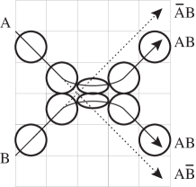
Figure 7: A collision in the Soft Sphere Model finitary CM dynamics.

5.1 Soft Sphere Model

In Figure 7 we illustrate the soft sphere model (SSM) [29]. The SSM is an invertible and energy conserving CM model of classical computation similar to Fredkin’s billiard ball model. Unlike the BBM, however, it can be turned into a lattice gas dynamics [32, 28] with point interactions.

As in the BBM we restrict the initial positions and velocities of balls to discrete values, to guarantee that the SSM acts like a digital system. In the collision shown in Figure 7, the horizontal component of velocity of all balls entering from the left is one column per time step, and so consecutive moments of the history of the collision occur in consecutive columns.

The collision shown is energy and momentum conserving and the compression and rebound takes exactly the time needed to displace the colliding balls from their original paths onto the paths labeled $AB$. If a ball had come in only at $A$ with no ball at $B$, it would leave along the path labeled $A\bar{B}$. This model is equivalent to a lattice gas automaton, with lattice sites located at the corners of the grid shown in the figure.

$$\begin{array}[]{c@{\hspace{.4in}}c}\includegraphics[height=108.405pt]{Figures/rel-coll5}\hfil\hskip 28.90755pt&\includegraphics[height=108.405pt]{Figures/rel-rule3}\\ \mbox{\bf(a)}\hfil\hskip 28.90755pt&\mbox{\bf(b)}\\ \end{array}$$

Figure 8: Rescalable soft sphere partitioning dynamics. (a) A time history of one column of particles colliding. At the times shown all particles are converging towards the center of the square they are in. (b) Site update rule. After the update particles are diverging from the center of the square. Only these cases interact (and rotations); otherwise particles go straight.

5.2 Rescalable SSM

Figure 8 describes the Rescalable Soft Sphere (RSS) model which implements a partitioning version of the SSM using colliding blocks of 1’s of any size. This is a new invertible model that conserves energy and momentum. Colliding blocks undergo collisions and then reform in appropriately shifted positions to exactly implement the SSM dynamics on any scale. The basic idea is that the size of the incoming blocks controls how long the interaction takes, because particles behave differently when they are surrounded by other particles than when they are alone. This allows the shift caused by a collision to depend on the size of the colliding blocks.

Figure 8a shows a simple collision. Two groups of three particles approach each other (first column on the left), with the top group moving right and down, the bottom group right and up. As in Figure 7, all particles have a constant horizontal velocity and so consecutive discrete moments in the history of the collision occur in consecutive columns.

Each square in Figure 8a is a block of the even-step partition and columns are shown at consecutive even times. This means that all particles within a square are converging towards the center of the square at the times shown. For example, since the top three black particles in the first column are in upper left squares, they are headed down and right. To make the diagram easier to understand we’ve spread out the particles in the initial state so that particles only ever interact on even steps, at the moments shown. The odd-step interaction is turned off for now—particles just go straight on odd steps. Later we’ll make both steps the same and put the particles closer together.

The size of the incoming groups of particles controls how long the interaction takes. Pairs of corresponding incoming black particles collide along the axis of symmetry between the incoming groups, each pair colliding at a separate spot. Each pair of colliding black particles turns into a pair of white particles moving in the same directions. The white particles move straight as long as they encounter other particles, but turn back towards the axis of the collision as soon as they find themselves alone. The white particles are labeled with a chirality ($+$ or $-$) at the time they are created, so that they will know which way to turn. The white particles ignore other white particles of the same chirality and don’t interact again until the $+$ and $-$ come back together at the axis of the collision. They then turn back into black particles and reconstitute two groups of black particles, each of which moves off as a unit.

5.3 Transition rule

The transition rule used in Figure 8a is shown in Figure 8b. On the left we see the particles before the interaction, as they converge towards the center of the square. On the right we show the particles after the interaction, as they diverge. In addition to the cases shown, each orthogonal rotation of a state on the left turns into the same rotation of the corresponding result case on the right. This allows us to have the same collision occur in any orthogonal orientation. In all cases not shown, there is no interaction. Particles go straight through the center of the square and continue moving in the same direction without change.

This rule can be inferred from Figure 8a. All of the cases shown are needed in order to reproduce the given evolution except for the second case (white to white collision) which doesn’t occur. This case is added to make the overall dynamics invertible. Since cases that aren’t shown don’t interact, particles will often pass through each other without affecting each other. For example, if two groups of black particles collide head on, they pass through each other. Since most of the “no interaction” cases don’t occur in the kind of collision shown in Figure 8a, we could augment the rule without affecting Figure 8a by changing some of the “no interaction” cases.

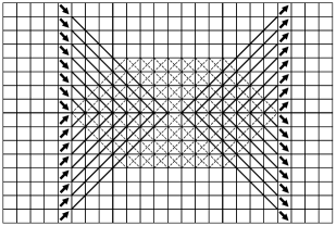
Figure 9: A larger collision in RSS dynamics. Two columns of 8 particles collide. Partitions are centered at middles and corners of the squares shown.

5.4 Square balls

Figure 9 shows a continuous time history for a collision of two groups of 8 incoming particles (black arrows on the left). The solid lines trace the paths of black particles, the dotted lines show the paths of white particles. Interactions occur at both the centers and the corners of the squares. The grid is shown with 8$\times$8 blocks of cells outlined by darker lines. Notice that the upper group of 8 incoming black particles occupies the fifth column within an 8$\times$8 block, and the corresponding outgoing group of black particles also occupies the fifth column within an 8$\times$8 block. Because of the uniform horizontal motion in this diagram, if we filled all of the columns in the two 8$\times$8 blocks on the left of the diagram with black particles (moving right and down in the top block, right and up in the bottom block), each input column would separately turn into the corresponding output column within the rightmost 8 columns. Thus two 8$\times$8 “square balls” would collide, reconstituting themselves one ball-width to the right of where the balls would have gone if no collision had occurred. Thus the RSS dynamics implements the Soft Sphere collision using square balls. By making balls square we allow them to sometimes collide along a horizontal axis and sometimes along a vertical axis—this couples the two dimensions.

5.5 Rescaling

If the square balls were larger, they would shift correspondingly further to the right: the block dynamics is scale invariant. The square ball dynamics scales all the way down to 1$\times$1 square balls: even single particles reproduce SSM collisions. We can take a Soft Sphere Model dynamics that is simulated at the finest grain size of the dynamics and reproduce it in a system $m$ times larger in each dimension at a rate $m$ times slower by simply replacing each block of the partition in the fine grain initial state by a tesselation of $m\times m$ identical blocks in the scaled system (cf. rescaling discussion in [23]).

Rescaling can be used as a way to take the continuum limit of an RSS model. If the time scale of the underlying RSS dynamics is $m$ times smaller than that of a scaled system, for $m$ sufficiently large the microscopic space and time scales can be considered infinitesimal compared to the “macroscopic” scales. At that point we have the macroscopic system performing a dynamics that is exactly equivalent to a microscopic dynamics, but in an effectively continuous space and time.

When macroscopic blocks collide, there is a question of which block is which afterwards. This of course depends on how we decide to interpret which particle is which when two particles collide. For example, if we decide that particle labels never cross the plane of a two-particle collision, then block collisions look like Figure 7 (repulsive collision). If we decide particle labels always cross, then entire blocks pass through each other as they come together and then again as they come apart (attractive collision).

$$\begin{array}[]{c@{\hspace{.6in}}c@{\hspace{.6in}}c}\includegraphics[height=90.3375pt,width=144.54pt]{Figures/rel-m-vs-t}\hfil\hskip 43.36243pt&\includegraphics[height=90.3375pt,width=144.54pt]{Figures/rel-y-vs-t}\hfil\hskip 43.36243pt&\includegraphics[height=90.3375pt]{Figures/rel-m-vs-r}\\ \mbox{\bf(a)}\hfil\hskip 43.36243pt&\mbox{\bf(b)}\hfil\hskip 43.36243pt&\mbox{\bf(c)}\\ \end{array}$$

Figure 10: Macroscopic limit of RSS collision (relativistic). (a) Fraction of energy that is mass, as a function of time. Three different conventions defining mass energy correspond to three different time-histories (solid-line, fine-dashed, coarse-dashed). (b) Vertical position $y$ of centers of the top and bottom balls as a function of time. (c) Fraction of energy that is mass, as a function of separation of ball centers.

5.6 1D and 3D

In Figure 9, we analyzed the collision of 2D blocks by observing that each column collides independently, as a 1D system. We could of course simply reinterpret the horizontal axis in the diagram as time, and this becomes a diagram of a 1D collision of two extended objects.

In this case blocks in the transition rule of Figure 8b should be half as wide: particles have only two directions (up and down). This is the only “rotation” of the rule in 1D. We still need two white particle types so that the white particles can pass through other white particles of the same type until the two different types come back together and collide at the “axis” of the collision.

To get the same rescalable SSM behavior in a 3D system we can simply apply the planar rule of Figure 8b in various orientations: only pairs of particles collide and the entire collision process takes place in the plane defined by the two particle directions. We need to use more kinds of labels for the white particles (more possibilities of which way they can turn), but for each collision plane only two kinds of turners are needed—these become the $+$ and $-$ particles in the rule. Of course the scalable 2D square balls become 3D cubical balls, and we only use a set of directions for which collisions occur between parallel faces of cubes.

5.7 Mass energy

Since the RSS model is a single-speed dynamics that conserves energy and momentum in its collisions, we are free to interpret it as a special case of a continuous classical relativistic dynamics with constrained initial conditions.

As two particles cross over the same spot in Figure 9, we can consider the continuation of each particle to be either the one that went straight or the one that turned. In the former case the particles move at the speed of light and are massless. In the latter case the net motion of each particle during the timestep is horizontal at less than the speed of light and so it has mass.

In this model all isolated freely moving particles have the same energy $\epsilon$, whose minimum possible value (Equation 17) sets the ideal energy scale. For a classical particle moving at the speed of light, $p=\epsilon/c$. In this section we use units in which $c=1$, so that the magnitude of the momentum equals the energy for a massless particle. For each particle that changes direction in a crossover the average momentum during the timestep is only $\epsilon/\sqrt{2}$ and so the mass is also $\epsilon/\sqrt{2}$, since $m^{2}=\epsilon^{2}-p^{2}$.

Thus during the collision of Figure 9, the mass goes from zero to a maximum of $8\sqrt{2}\epsilon$ and then back to zero. In units of $\sqrt{2}\epsilon$, the mass at each step of the collision is just the number of mass-generating crossings in a column. A collision of two $n\times n$ square balls corresponds to $n$ simultaneous collisions such as the one in the figure. As we let the balls get larger and larger, the fraction of the total energy that is mass energy approaches one of the three curves shown in Figure 10a.

Here we’ve chosen our unit of time to be the time it takes a freely moving square ball to move the length of its diagonal. With this unit, a collision takes two units of time. Because of the symmetry of the collision, the fraction of the energy that is mass is the same for each of the two colliding balls: each ball changes energy into mass and then back again according to the curves shown.

Which curve the mass of each ball follows depends on how we interpret the particle crossings. We’ve shown three possible interpretations. The “maximum mass” interpretation, (coarse-dashed line) is given as a function of time by considering all crossings to be massive. The “sudden mass” interpretation (thick-solid line) interprets all particles of each square ball as moving straight (with perhaps a change in particle-type) until the moment the two balls completely overlap, and then all crossings have mass until the two balls start to separate. The “white mass” interpretation (fine-dashed line) is given by only counting pairs of white particles that cross to be massive. The “maximum mass” interpretation corresponds to the minimum possible motion (least kinetic energy).

Let us associate the entire mass of each ball with a single representative point. For a freely moving ball, the representative point is the center of the ball. Since $E=\gamma M$ the ratio of mass to energy shown in Figure 10a is equal to $1/\gamma$. Knowing $\gamma$ as a function of time gives us the velocity $v$ of the ball as a function of time. Since the horizontal component of $v$ is unaffected by the collision and remains constant this gives us the vertical velocity as a function of time, and hence the vertical position as a function of time. This is depicted in Figure 10b, where we’ve shown the path that the representative point for each ball must follow during a collision if its mass varies according to one of the three curves in Figure 10a. The three cases show that exactly the same collision can be interpreted as attractive, repulsive, or sticky.

It is clear from the behavior of $M/E$ and $y$ as functions of time that the ratio $M/E$ depends only on the separation $r$ between the two representative points (once the interaction starts). This dependence is graphed in Figure 10c. Thus if we think of mass as a kind of relativistic potential energy (i.e., total energy minus kinetic energy), we see that it depends only on the distance between the two balls. The potential is zero when the balls are not yet close enough to touch and it increases as the balls collide. The maximum mass $M$ for each ball is the fraction $E/\sqrt{2}$ of the ball’s energy, which obtains when all particles are paired so that there is maximum cancellation of vertical momentum components.

5.8 Relativistic invariance?

We were able to use the RSS model to discuss mass in a relativistic collision by interpreting the model’s single particle-speed as the speed of light and its conservations as relativistic conservations. This model is, however, clearly not very relativistic even in a continuum limit. While it does display macroscopic mechanical behavior, it does so only in a single inertial frame. It thus does not exhibit relativistic frame invariance.

We might expect that, for a colliding pair of RSS particles, the relativistic kinetic energy (which includes only energy related to net translational motion) should be closely related to the state-change energy (which is the minimum energy for the net motion). This suggests that we might be able to use the intrinsic definition of ideal kinetic energy provided by state-change to expose the non-relativistically invariant character of the RSS model.

If we interpret freely moving RSS particles as massless, as we did in Section 5.7, then state-change energy and relativistic kinetic energy evolve differently. The state-change energy of both a free particle and of a block where two particles cross are the same (Equation 17). In constrast, if the relativistic kinetic energy of a free massless particle is $\epsilon$, then the relativistic kinetic energy of a block containing two massless particles whose paths intersect at right angles is only $2\epsilon(1-1/\gamma)\approx.6\epsilon$.

We can try to reinterpret the RSS dynamics to make the relativistic kinetic energy match the state-change energy both for a free particle and for a two-particle collision. If we let free RSS particles each have mass $m_{f}$ and let a two-particle collision have mass $m_{c}$ we find that the only choice of masses that allows the two energies to be equal is $m_{c}=2m_{f}$, which corresponds to $\gamma=1$. Thus the state-change energy becomes the ideal kinetic energy in the RSS model only for a non-relativistic interpretation of the dynamics.

6 Conclusions

A finite-sized QM system has only a finite number of possible distinct states and can move between distinct states at only a finite rate. This means that classical special cases of QM dynamics must be classical finite-state dynamics. Conversely, we can regard the dynamics of real physical systems to be a generalization of classical finite-state dynamics. This is not a common viewpoint among physicists today.

The study of classical finite-state dynamics that are special cases of QM dynamics should, at the least, be of interest for pedagogical reasons since it allows physical concepts to be seen in an intuitive classical setting. This study should also be of interest to theoretical computer science since it establishes an exact correspondence between a classical computation and an ideal quantum realization. Finally, this study should be of interest to theoretical physics since it provides a novel finite-state perspective on the foundations of both classical and quantum mechanics, along with an intuitive starting point for the construction of new physical models.

References

- [1] A. Barenco, C. H. Bennett, R. Cleve, D. P. DiVincenzo, N. Margolus, P. Shor, T. Sleator, J. A. Smolin, and H. Weinfurter, “Elementary gates for quantum computation,” Phys. Rev. A 52:5, 3457–3467 (1995), arXiv:quant-ph/9503016.
- [2] S. I. Ben-Abraham, “Curious properties of simple random walks,” J. Stat. Phys. 73: 441–445 (1993).
- [3] P. Benioff, “Quantum Mechanical Hamiltonian Models of Computers,” Annals of the New York Academy of Sciences 480:1, 475–486 (1986).
- [4] C. H. Bennett, “Logical Reversibility of Computation,” IBM J. Res. Develop. 6, 525–532 (1973).
- [5] C. H. Bennett and D. P. DiVincenzo, “Quantum Information and Computation,” Nature 404:6775, 247–255 (2000).
- [6] I. Bialynicki-Birula, “Weyl, Dirac and Maxwell equations on a lattice as unitary cellular automata,” Phys. Rev. D 49:12, 6920–6927 (1994).
- [7] I. Bialynicki-Birula, “Photon Wave Function,” in Progress in Optics XXXVI (E. Wolf, ed.), Elsevier, 245–294 (1996).
- [8] H. W. J. Blöte, E. Luijten and J. R. Heringa, “Ising universality in three dimensions: A monte-carlo study,” J. Phys. A 28, 6289 (1995), arXiv:cond-mat/9509016.
- [9] B. M. Boghosian and W. Taylor, “Simulating Quantum Mechanics on a Quantum Computer,” Physica D 120 30-42 (1998).
- [10] G. Caterina and B. Boghosian, “A ‘No-Go’ Theorem for the Existence of an Action Principle for Discrete Invertible Dynamical Systems,” arXiv:nlin/0611058 (2006).
- [11] E. Fredkin, R. Landauer and T. Toffoli (eds.), Proceedings of the Physics of Computation Conference, in Int. J. Theor. Phys., issues 21:3/4, 21:6/7, and 21:12 (1982).
- [12] E. Fredkin and T. Toffoli, “Conservative logic,” in [11, p. 219–253].
- [13] E. Fredkin, “Five big questions with pretty simple answers,” IBM J. Res. & Dev. 48:1, 31–45.
- [14] E. Fredkin, “A computing architecture for physics,” Proceedings of the 2nd conference on computing frontiers, ACM New York NY, 273–279 (2005).
- [15] R. Gambini and J. Pullin, “Classical and quantum general relativity: a new paradigm,” General Relativity and Gravitation 37:10, 1689–1694 (2005), arXiv:gr-qc/0505052.
- [16] H. Hrgovčić, “Discrete representations of the n-dimensional wave equation,” J. Phys. A: Math. Gen. 25, 1329–1350 (1992).
- [17] S. Ihara, Information theory for continuous systems, World Scientific, Chapter 3 (1993).
- [18] H. Ikeda and K. Hirakawa, “Neutron scattering study of two-dimensional Ising nature of K2CoF4,” Solid State Communications, vol 14 529–532 (1974).
- [19] L. Kauffman and H. P. Noyes, “Discrete physics and the Dirac equation,” Phys. Lett. A 2:18 139–146 (1996), arXiv:hep-th/9603202.
- [20] J. P. Keener, Principles of Applied Mathematics: Transformation and Approximation, Westview Press, Chapter 7 (2000).
- [21] J. Koenderink, “The structure of images,” Biological Cybernetics 50:5, 363–370 (1984).
- [22] T. D. Lee and C. N. Yang, “Statistical theory of equations of state and phase transitions. II. Lattice gas and Ising model,” Phys. Rev. 87:3 410–419 (1952).
- [23] N. Margolus, “Physics-like models of computation,” Physica D 10:1/2 (1984).
- [24] N. Margolus, “Quantum computation,” in New Techniques and Ideas in Quantum Measurement Theory (Daniel Greenberger, ed.), New York Academy of Sciences, 487–497 (1986).
- [25] N. Margolus, T. Toffoli and G. Vichniac, “Cellular-Automata Supercomputers for Fluid Dynamics Modeling,” Phys. Rev. Lett. 56 1694–1696 (1986).
- [26] N. Margolus, “Parallel quantum computation,” in Complexity, Entropy and the Physics of Information (W. H. Zurek, ed.), Addison-Wesley New York, 273–287 (1990).
- [27] N. Margolus and L. Levitin, “The maximum speed of dynamical evolution,” Physica D 120:1/2, 188–195 (1998), arXiv:quant-ph/9710043.
- [28] N. Margolus, “Crystalline Computation,” in Feynman and Computation (Hey, ed.), Perseus Books Reading MA, 267–305 (1998), arXiv:comp-gas/9811002.
- [29] N. Margolus, “Universal cellular automata based on the collisions of soft spheres,” in D. Griffeath and C. Moore, (eds.), New Constructions in Cellular Automata, Oxford University Press, 231–260 (2003), arXiv:0806.0127.
- [30] D. A. Meyer, “From quantum cellular automata to quantum lattice gases,” J. Stat. Phys. 85, 551–574 (1996); arXiv:quant-ph/9604003.
- [31] E. Meijering, “A chronology of interpolation: from ancient astronomy to modern signal and image processing,” Proc. IEEE 90:3, 319–342 (2002).
- [32] D. Rothman and S. Zaleski, Lattice Gas Cellular Automata: Simple Models of Complex Hydrodynamics, Cambridge University Press, (2004).
- [33] D. Ruelle, Statistical Mechanics: Rigorous Results, World Scientific, (1999).
- [34] M. Smith, “Representation of geometrical and topological quantities in cellular automata,” Physica D 45, 271–277 (1990).
- [35] F. Stenger, “Numerical methods based on Whittaker cardinal, or sinc, functions,” SIAM Review 23:2, 165–224 (1981).
- [36] G. ’t Hooft, “Equivalence relations between deterministic and quantum mechanical systems,” J. Stat. Phys. 53:1/2, 323–344 (1988).
- [37] G. ’t Hooft, “Quantum Mechanical behaviour in a deterministic model,” Found. Phys. Lett. 10 105–111 (1997), arXiv:quant-ph/9612018.
- [38] G. ’t Hooft, “A mathematical theory for deterministic quantum mechanics,” Journal of Physics: Conference Series 67:1, 012015 (2007).
- [39] T. Toffoli, “Cellular automata as an alternative to (rather than an approximation of) differential equations in modeling physics,” Physica D 10:1/2, 117–127 (1984).
- [40] T. Toffoli, “Action, or the fungibility of computation,” in Feynman and computation: exploring the limits of computers (A. Hey ed.), Perseus Books, 349–392 (1999).
- [41] J. C. Wheeler, “Decorated lattice-gas models of critical phenomena in fluids and fluid mixtures,” Ann. Rev. Phys. Chem. 28, 411–443 (1977).
- [42] S. Wolfram, A New Kind Of Science, Wolfram Media Inc, (2002).
- [43] J. Yepez, “Relativistic Path Integral as a Lattice-based Quantum Algorithm,” Quantum Information Processing 4:6, 471–509 (2005).
- [44] J. M. Ziman, Elements of Advanced Quantum Theory, Cambridge University Press, Section 2.2 (1969).