$\mathrm{P^{3}M}$ algorithm for dipolar interactions

Abstract

An extension to the $\mathrm{P^{3}M}$ algorithm for electrostatic interactions is presented, that allows to efficiently compute dipolar interactions in periodic boundary conditions. Theoretical estimates for the root-mean square error of the forces, torques and the energy are derived. The applicability of the estimates is tested and confirmed in several numerical examples. A comparison of the computational performance of the new algorithm to a standard dipolar Ewald summation methods shows a performance crossover from the Ewald method to the dipolar $\mathrm{P^{3}M}$ method for as few as 300 dipolar particles. In larger systems, the new algorithm represents a substantial improvement in performance with respect to the dipolar standard Ewald method. Finally, a test comparing point-dipole based and charged-pair based models shows that point-dipole based models exhibit a better performance than charged-pair based models.

I Introduction

Dipolar interactions are important in many soft-matter systems ranging from dispersions of magnetic micro- and nanoparticles (ferrofluids) and electrorheological fluids to magnetic thin films and water odenbach02a ; rosensweig85a ; berkovsky93a ; berkovsky96a ; holm05b ; weis05a . Numerical simulations play a central role in explaining and unravelling the rich variety of new and unexpected behavior found in recent theoretical and experimental studies on dipolar systems blums97a ; odenbach02b . Especially for systems which possess point-dipolar interactions such as dipolar model systems used in analytical theories, or ferrofluids, a numerical algorithm based on truly dipolar interactions is needed holm05b ; weis05a . Periodic boundary conditions are frequently used in these simulations in order to approach bulk systems within the limits of currently available computers (see ref. heinz05a for a detailed discussion about the adequacy of such methods to describe electrostatic systems). If a system of $N$ particles with positions $\left\{\bm{r}_{i}\right\}_{i=1}^{i=N}$ in a cubic box of length $L$ that carry point dipoles $\{\bm{\mu}_{i}\}_{i=1}^{i=N}$ is considered, then the total electrostatic energy under periodic boundary conditions is given, in Gaussian units, by

$$U=\frac{1}{2}\sum_{i=1}^{N}\sum_{j=1}^{N}\sideset{}{{}^{{}^{\prime}}}{\sum}_{\bm{n}\in\mathbb{Z}^{3}}v(\bm{r}_{ij}+\bm{n}L,\bm{\mu}_{i},\bm{\mu}_{j})$$ (1)

where $\bm{r}_{ij}=\bm{r}_{i}-\bm{r}_{j}$, and

$$v(\bm{r}_{ij},\bm{\mu}_{i},\bm{\mu}_{j})\equiv(\bm{\mu}_{i}\cdot\nabla_{\bm{r}_{i}})\left(\bm{\mu}_{j}\cdot\nabla_{\bm{r}_{j}}\right)\frac{1}{|\bm{r}_{ij}|}$$

$$\phantom{v(\bm{r}_{ij},\bm{\mu}_{i},\bm{\mu}_{j})}=\frac{\bm{\mu}_{i}\cdot\bm{\mu}_{j}}{|\bm{r}_{ij}|^{3}}-\frac{3\left(\bm{\mu}_{i}\cdot\bm{r}_{ij}\right)\left(\bm{\mu}_{j}\cdot\bm{r}_{ij}\right)}{|\bm{r}_{ij}|^{5}}$$ (2)

is the dipolar pair interaction for point dipoles. The innermost sum runs over all periodic images of the system, identified by the shifting integer vector $\bm{n}$. The prime in the sum in eq. (1) indicates that the $i=j$ term must be omitted for $\bm{n}=0$. Note that the dipolar sum is conditionally convergingdeLeeuw80a and its precise value depends on the summation order. In what follows we assume eq. (1) to be summed over spherical shells (spherical order of summation)deLeeuw80a ; deLeeuw80b .

The force $\bm{F}_{i}$, and the electrostatic field $\bm{E}_{i}$ acting on a particle $i$ can be obtained by differentiating the potential energy $U$ with respect to ${\bm{r}}_{i}$ and $\bm{\mu}_{i}$ respectively, i.e.,

$$\bm{F}_{i}=-\nabla_{\bm{r}_{i}}U$$ (3)

$$\bm{E}_{i}=-\nabla_{\bm{\mu}_{i}}U.$$ (4)

In the case of dipoles, these quantities are related via $\bm{F}(\bm{r})=\nabla_{\bm{r}}(\bm{\mu}\cdot\bm{E}(\bm{r}))$. For point-dipoles, the torque $\bm{\tau}_{i}$ acting on particle $i$ can be related to the electrostatic field at the position of the particle as

$$\bm{\tau}_{i}=\bm{\mu}_{i}\times\bm{E}_{i}$$ (5)

Performing the direct summation of the interactions (eq. (1)) is impracticable beyond a few particles due to the slow convergence of the innermost sum and the quadratic scaling with the total number $N$ of particles in the outer sums. However, algorithms have been proposed to speed up the computation of dipolar interactions: the dipolar Ewald sum allen87a ; wang01a , the dipolar Lekner sum weis05a , the (Smooth) Particle-Mesh Ewald methods: PME and SPME toukmaji00a , and Multipole Methods (MM): Fast-MM, and Cell-MM kutteh95a ; kutteh95b ; stoycheva02a ; christiansen93a . For a general overview of these algorithms, see the reviews in refs. weis05a ; arnold05a .

Although the Ewald summation is significantly better than direct summation from a computational point of view, it still exhibits an unfavourable $\mathcal{O}(N^{3/2})$ scaling with the number of particles perram88 . By contrast, Multipole methods scale linearly, but have a large prefactor in the $\mathcal{O}(N)$ scaling. In the case of point charges, Multipole methods have been found to be superior to mesh methods only for very large systems $N\geq 100000$ (see discussion in ref. petersen95a and sagui99a ). For systems of moderate size, optimal algorithms are those that take advantage of the Fast Fourier Transform ($\mathrm{FFT}$) in order to compute the Fourier contribution to the Ewald sum, which are commonly known as particle mesh methods: PME, SPME, and Particle-Particle-Particle Mesh ($\mathrm{P^{3}M}$), which is introduced in this article. These methods are all $\mathcal{O}(N\log N)$, i.e. they exhibit a nearly linear scaling with the number of particles.

When computing Coulomb interactions, the $\mathrm{P^{3}M}$ method hockney81a achieves the highest accuracy among the particle mesh methods, thanks to its use of the optimal lattice Green function that is designed to minimize root-mean-square (rms) errors deserno98a ; sagui99 . The PME and SPME algorithms have already been generalized to compute dipolar interactions toukmaji00a . In this paper we perform a similar generalization, but for the $\mathrm{P^{3}M}$ algorithm. An advantage of the $\mathrm{P^{3}M}$ approach is that it provides theoretical estimates for the rms accuracy of the forces, torques and energy as by-products. These estimates give valuable information about the accuracy of the algorithm without having to perform tedious benchmarking, and they allow for the tuning of the algorithm to yield minimal computing time at a given level of accuracy. No such theoretical error estimates are currently known for the dipolar PME nor SPME methods.

To verify the applicability and correctness of the method presented in this article and to be able to perform the numerical tests, the method was implemented in the simulation package ESPResSolimbach06a ; espressoweb , and it will be contained in one of the coming releases of the software.

The outline of this paper is as follows. The basic formulas for the Ewald summation of dipolar interactions are recalled in Sct. II.1. In Sct. II.2, Hockney and Eastwoods’s $\mathrm{P^{3}M}$ algorithm is extended to compute dipole-dipole interactions. A correction term that must be applied to any dipolar energy when computed via particle-mesh-methods is derived in Sct. II.3. Theoretical estimates for the rms error of forces, torques, and energy as computed by $\mathrm{P^{3}M}$ are presented in Sct. III. Numerical tests of the accuracy of the error estimates are made in Sct. IV. In Sct. V several issues related to the computational efficiency of the method are discussed: performance of the method when compared to the traditional dipolar Ewald sums, suitable approaches to make a fast implementation of the method in constant-pressure simulations, and a comparison of the efficiency of dipole-based and charge-based models to mimic dipolar systems. Technical details for building up the $\mathrm{P^{3}M}$ dipolar method are given in App. A, while App. B derives and discusses the rms error estimates.

II The dipolar $\mathrm{P^{3}M}$ method

In this section the dipolar $\mathrm{P^{3}M}$ algorithm is presented by first recalling the basics of the dipolar Ewald summation in which the new method has its roots (see Sct. II.1). The details of the new algorithm are presented in Sct. II.2. The effect of discretization errors in Madelung-Self interactions (those of a particle with its periodic images and itself) is discussed and a correction term to remove a bias in the energy is derived in Sct. II.3. The different Fourier Transforms as well as the domains to which they apply are defined in Table I. In the following, we assume a cubic box, but the generalization to triclinic boxes is straightforward, see for instance ref. toukmaji00a for an implementation in PME and SPME algorithms.

II.1 Ewald summation with dipolar interactions

The fundamental idea of the Ewald summation (and its advanced implementations like the particle mesh methods PME, SPME and $\mathrm{P^{3}M}$) is to calculate energies, forces, and torques by splitting the long-ranged dipolar pair-interaction into two parts,

$$v(\bm{r},\bm{\mu}_{i},\bm{\mu}_{j})=\left(\bm{\mu}_{i}\cdot\nabla_{\bm{r}_{i}}\right)\left(\bm{\mu}_{j}\cdot\nabla_{\bm{r}_{j}}\right)\big{(}\psi(\bm{r}_{ij})+\phi(\bm{r}_{ij})\big{)},$$ (6)

where $\psi(\bm{r})$ contains the short-distance part of the Coulomb interaction, and $\phi(\bm{r})$ contains its long-distance part ($\phi(\bm{r})$ must moreover be smooth everywhere and regular at the origin). The standard way to perform this splitting is to set

$$\psi(\bm{r})\equiv\frac{\mathrm{erfc}(\alpha r)}{r},\qquad r=|\bm{r}|,$$ (7)

$$\phi(\bm{r})=\frac{\mathrm{erf}(\alpha r)}{r},$$ (8)

though other choices are possible ewald21 ; rajagopal94 ; hunenberger00a ; batcho01a . The inverse length $\alpha$, which is often referred to as the Ewald (or splitting) parameter, weighs the importance of one term with respect to the other, and can be chosen so as to optimize the performance. The interactions associated to the function $\psi$ are short-ranged and they can hence efficiently be summed numerically. The interactions associated to the function $\phi$ are long-ranged in real space, but short-ranged in the reciprocal Fourier space, and can therefore be efficiently computed in that latter space. The decomposition of the potential leads to the well-known Ewald formula for the electrostatic energy of a system of dipoles (see details in refs weis05a ; frenkel02a ; deLeeuw80a ; deLeeuw80b )

$$U=U^{(r)}+U^{(k)}+U^{\mathrm{(self)}}+U^{\mathrm{(surf)}}$$ (9)

where the real-space energy $U^{(r)}$, the reciprocal-space energy $U^{(k)}$, the self-energy $U^{\mathrm{(self)}}$ and the surface $U^{\mathrm{(surf)}}$ contributions are

$$U^{(r)}=\frac{1}{2}\sum_{i,j=1}^{N}\sideset{}{{}^{{}^{\prime}}}{\sum}_{\bm{n}\in\mathbb{Z}^{3}}(\bm{\mu}_{i}\cdot\nabla_{\bm{r}_{i}})\left(\bm{\mu}_{j}\cdot\nabla_{\bm{r}_{j}}\right)\psi(\bm{r}_{ij})$$ (10)

$$U^{(k)}=\frac{1}{2V}\sum_{\bm{k}\neq 0\atop\bm{k}\in\mathbb{K}^{3}}|\hat{\bm{\rho}}(\bm{k})\cdot i\bm{k}|^{2}\breve{\phi}(\bm{k})$$ (11)

$$U^{\mathrm{(self)}}=-\frac{2\alpha^{3}}{3\sqrt{\pi}}\sum_{i=1}^{N}\mu_{i}^{2}$$ (12)

$$U^{\mathrm{(surf)}}=\frac{2\pi}{(2\epsilon^{\prime}+1)V}\sum_{i=1}^{N}\sum_{j=1}^{N}\bm{\mu}_{i}\cdot\bm{\mu}_{j},$$ (13)

where $V=L^{3}$ is the volume of the box, and $\epsilon^{\prime}$ is the dielectric constant of the medium surrounding the replica boxes: $\epsilon^{\prime}=1$ for vacuum, and $\epsilon^{\prime}=\infty$ for metallic boundary conditions. Because of the periodic boundary conditions, wave vectors $\bm{k}\in{\mathbb{K}}^{3}$ are discrete where ${\mathbb{K}}^{3}\equiv\{2\pi\bm{n}/L:\bm{n}\in{\mathbb{Z}}^{3}\}$. In Eq. (11), $\hat{\bm{\rho}}(\bm{k})$ is the Fourier transform of the periodic dipole density

$$\bm{\rho}(\bm{r})=\sum_{i=1}^{N}\bm{\mu}_{i}\,\delta(\bm{r}-\bm{r}_{i}),\qquad\bm{r}\in V,$$ (14)

which reads,

$$\hat{\bm{\rho}}(\bm{k})\equiv\mathrm{\mathrm{FT}}[\bm{\rho}](\bm{k})=\sum_{i=1}^{N}\bm{\mu}_{i}\,e^{-i\bm{k}\cdot\bm{r}_{i}}.$$ (15)

In (11), the Fourier transform $\breve{\phi}(\bm{k})$ of the reciprocal interaction (8) is

$$\breve{\phi}(\bm{k})=\int\!\phi(\bm{r})e^{-i\bm{k}\cdot\bm{r}}\mathrm{d}\bm{r}=\frac{4\pi}{k^{2}}e^{-k^{2}/4\alpha^{2}}.$$ (16)

The term $U^{\mathrm{(self)}}$ subtracts the unwanted self-energies that are included in the reciprocal energy $U^{(k)}$, where the self-energy of a dipole is defined as the reciprocal interaction of the dipole with itself: $\lim_{\bm{r}\rightarrow 0}(-\frac{1}{2})\left(\bm{\mu}_{i}\cdot\nabla_{\bm{r}}\right)^{2}\phi(\bm{r})$. It should be remarked that the expression given in eq. (13) for the surface term is valid only when a spherical order of summation is used in the calculation of the direct sumdeLeeuw80a ; deLeeuw80b , eq. (1). In that case, eqs. (1) and eq. (9) lead to identical values, provided that the interaction energy of the dipoles with the surrounding medium of dielectric constant $\epsilon^{\prime}$ at infinity is added to eq. (1) ($\epsilon^{\prime}=1$ was assumed when writing (1)). Notice that the surface term vanishes if metallic boundary conditions ($\epsilon^{\prime}=\infty$) are used.

Ewald expressions for the force and electric field acting on a dipole $i$ follow from eqs. (3), (4) and (9):

$$\bm{F}_{i}=\bm{F}^{(r)}_{i}+\bm{F}^{(k)}_{i}$$ (17)

$$\bm{E}_{i}=\bm{E}^{(r)}_{i}+\bm{E}^{(k)}_{i}+\bm{E}^{\mathrm{(self)}}_{i}+\bm{E}^{\mathrm{(surf)}}_{i}.$$ (18)

where the superscripts $(r)$ and $(k)$ denote the real-space and reciprocal-space contributions. Notice that there is no self- nor surface-contribution to the force because the self- and surface-energy terms (eqs. (12) and (13)) are independent of the particle positions. By (5), the torque on dipole $i$ follows directly from the electric field: $\bm{\tau}_{i}=\bm{\mu}_{i}\times\bm{E}_{i}$. The reader is referred to ref. wang01a for fully explicit Ewald formulas for the real space and reciprocal space contributions to the force and torque. For further reference, it is worth noting that the reciprocal space contributions to the force and electrostatic field can be written as

$$\bm{E}^{(k)}_{i} = {\mathrm{FT}}^{-1}_{\bm{k}\neq 0}\left[\hat{\bm{E}}^{(k)}\right]={\mathrm{FT}}^{-1}_{\bm{k}\neq 0}\left[i\bm{k}\left(\hat{\bm{\rho}}(\bm{k})\cdot i\bm{k}\right)\breve{\phi}(\bm{k})\right]$$ (19)

$$\bm{F}^{(k)}_{i} = {\mathrm{FT}}^{-1}_{\bm{k}\neq 0}\left[i\bm{k}(\bm{\mu}_{i}\cdot i\bm{k})\left(\hat{\bm{\rho}}(\bm{k})\cdot i\bm{k}\right)\breve{\phi}(\bm{k})\right]$$

$$= \,\mu_{i,x}\,{\mathrm{FT}}^{-1}_{\bm{k}\neq 0}\left[\hat{{E}}_{x}^{(k)}~{}i\bm{k}\right]\,+\mu_{i,y}\,{\mathrm{FT}}^{-1}_{\bm{k}\neq 0}\left[\hat{{E}}_{y}^{(k)}~{}i\bm{k}\right]\,+\mu_{i,z}\,{\mathrm{FT}}^{-1}_{\bm{k}\neq 0}\left[\hat{{E}}_{z}^{(k)}~{}i\bm{k}\right]$$

$$= \,\mu_{i,x}\,{\mathrm{FT}}^{-1}_{\bm{k}\neq 0}\left[\hat{\bm{E}}^{(k)}~{}ik_{x}\right]\,+\mu_{i,y}\,{\mathrm{FT}}^{-1}_{\bm{k}\neq 0}\left[\hat{\bm{E}}^{(k)}~{}ik_{y}\right]\,+\mu_{i,z}\,{\mathrm{FT}}^{-1}_{\bm{k}\neq 0}\left[\hat{\bm{E}}^{(k)}~{}ik_{z}\right]$$

where the inverse Fourier series $\mathrm{\mathrm{FT}}^{-1}[\cdots]$ is defined in Table I (the $\bm{k}=0$ term must be excluded in the back-transformation), and the components of the Fourier transform of the electrostatic field are $\hat{\bm{E}}^{(k)}=(\hat{{E}}_{x}^{(k)},\hat{{E}}_{y}^{(k)},\hat{{E}}_{z}^{(k)})$, and $\bm{\mu}_{i}=(\mu_{i,x}\,,\mu_{i,y}\,,\mu_{i,z})$ is the dipole moment of particle $i$. The last equality for the force arises from the fact that $\bm{F}(\bm{r})=\nabla_{\bm{r}}(\bm{\mu}\cdot\bm{E}(\bm{r}))=(\bm{\mu}\cdot\nabla_{\bm{r}})\bm{E}(\bm{r})$ in electrostatics ($\nabla\times\bm{E}=0$).

From a computational point of view, the Ewald method requires therefore to first Fourier transform the dipole distribution to the reciprocal space, then to solve the Poisson equation in reciprocal space [which reduces to a simple multiplication by $\breve{\phi}(\bm{k})$], and finally to Fourier-back-transform the results to real space.

II.2 Algorithmic details of the mesh calculations

What distinguishes the particle mesh methods from the Ewald summation is that, while Ewald summation uses the standard Fourier series to compute the reciprocal space contribution, particle mesh methods use Fast Fourier Transformations ($\mathrm{FFT}$), thereby reducing the computational effort from ${\cal O}(N^{3/2})$ to ${\cal O}(N\log N)$. However, since $\mathrm{FFT}$ is a mesh transformation, it is necessary to: (1) Map the dipole moments from continuous positions onto lattice points (which will be referred to as dipole assignment to the mesh sites); (2) Fast-Fourier transform the mesh and solve the Poisson equation on the (reciprocal) mesh; (3) Fourier transform the mesh back to real-space, and interpolate the results onto the continuous dipole positions.

The computation of the real-space contribution $U^{(r)}$ in the Ewald formula is kept unchanged, and the reader is referred to wang01a for explicit formulas. In the following, we discuss in detail the mesh calculation in the case where the $i\bm{k}$-differentiation scheme is used. Other differentiation schemes can be easily implemented, see deserno98a for details.

The mesh is assumed to be a cubic FFT mesh with the lattice spacing given by $h=L/N_{M}$, where $N_{M}$ stands for the number of mesh points in each direction. We denote by ${\mathbb{M}}^{3}$ the set of all points belonging to the mesh: ${\mathbb{M}}^{3}\equiv\{\bm{n}h:\bm{n}\in{\mathbb{Z}}^{3},0\leq n_{x,y,z}<N_{M}\}$. An index ‘M’ is attached to any quantity defined at mesh points only, e.g. the mesh-based dipole density $\rho_{M}(\bm{r}_{m})$ or the mesh-based electric field $\bm{E}_{M}(\bm{r}_{m})$, $\bm{r}_{m}\in\mathbb{M}^{3}$. The inverse fast Fourier transform FFT${}^{-1}[\widetilde{f}]$ corresponds to a truncated Fourier series over wave vectors in one Brillouin zone (see Table I ). By convention, this zone is taken to be the set of wave vectors $\widetilde{\mathbb{M}}^{3}\equiv\{2\pi{\bm{n}}/L:\bm{n}\in{\mathbb{Z}}^{3},|n_{x,y,z}|<N_{M}/2\}$, which we call the “reciprocal mesh” or first Brillouin zone. The number of mesh points per direction $N_{M}$ should preferably be a power of two, because in that case the FFTs are computed more efficiently. Notice that with this definition, the reciprocal mesh is symmetric: if wave vector $\bm{k}$ belongs to the mesh, so does $-\bm{k}$.

II.2.1 Dipole assignment

The dipole density $\bm{\rho}_{M}(\bm{r}_{m})$ on the mesh is determined from the $N$ dipolar particles $\{(\bm{r}_{i},\bm{\mu}_{i})\}$ by the assignment function $W(\bm{r})$ that maps the particles from their continuous positions to the mesh,

$$\ \bm{\rho}_{M}(\bm{r}_{m})=\frac{1}{h^{3}}\sum_{i=1\atop\emph{m.i.c.}}^{N}\bm{\mu}_{i}W(\bm{r}_{m}-\bm{r}_{i}),$$ (21)

where minimum image convention (m.i.c.) is used when computing relative distances $\bm{r}_{m}-\bm{r}_{i}$. We use the same assignment functions $W(\bm{r})$ as defined by Hockney and Eastwood in the original $\mathrm{P^{3}M}$ method for Coulomb interactionshockney81a , which are (shifted) B-splines and are tabulated in ref. deserno98a . The assignment functions are classified according to the number $P$ of nearest grid points per coordinate direction over which the dipole is distributed. The quantity $P$ is referred to as the assignment order parameter. A formal expression for Hockney and Eastwood’s assignment functions is $W^{(P)}({\bm{r}})=W^{(P)}(x)W^{(P)}(y)W^{(P)}(z)$ where

$$W^{(P)}(x)=\underbrace{\left(\chi[\frac{-1}{2},\frac{1}{2}]\star...\star\chi[\frac{-1}{2},\frac{1}{2}]\right)}_{P\mathrm{-fold-convolution}}\left(\frac{x}{h}\right)$$ (22)

and $\chi[\frac{-1}{2},\frac{1}{2}]$ is the characteristic function, i.e., the function that is $1$ within this interval and $0$ outside.

II.2.2 Solving the Poisson equation

The reciprocal electrostatic energy, and electrostatic field are computed at each mesh point $\bm{r}_{m}$ by approximating equations (11), and (19) by

$$U^{(k)}_{M}=\frac{1}{2V}\sum_{\bm{k}\in\widetilde{\mathbb{M}}^{3}\atop\bm{k}\neq 0}\left|\widetilde{\bm{\rho}}_{M}(\bm{k})\cdot\widetilde{\bm{D}}(\bm{k})\right|^{2}\widetilde{G}(\bm{k})$$ (23)

$$\bm{E}^{(k)}_{M}(\bm{r}_{m})=\mathrm{FFT}^{-1}_{\bm{k}\neq 0}\left[\widetilde{\bm{E}}^{(k)}_{M}\right]=\mathrm{FFT}^{-1}_{\bm{k}\neq 0}\left[\widetilde{\bm{D}}(\bm{k})\left(\widetilde{\bm{\rho}}_{M}(\bm{k})\cdot\widetilde{\bm{D}}({\bm{k}})\right)\widetilde{G}(\bm{k})\right](\bm{r}_{m}).$$ (24)

Here, $\widetilde{\bm{\rho}}_{M}(\bm{k})$ is the fast Fourier transform of the dipole density $\bm{\rho}_{M}(\bm{r})$ on the mesh. The $\bm{k}=0$ term is excluded in the inverse transform FFT^-1 of all mesh-based quantities as in reciprocal Ewald terms eqs. (11), (19), and (II.1). The function

$$\widetilde{\bm{D}}(\bm{k})=i\bm{k},\qquad\bm{k}\in\widetilde{\mathbb{M}}^{3},$$ (25)

is the Fourier expression of the gradient operator on the reciprocal mesh. $\widetilde{G}(\bm{k})$ is the lattice Green function, also known as the influence function, and it is defined below at the end of Sec. B [see eq. (30)]. It should be remarked that both $\widetilde{\bm{D}}(\bm{k})$ and $\widetilde{G}(\bm{k})$ are periodic in $\widetilde{\mathbb{K}}^{3}$, with the period given by the first Brillouin cell $\widetilde{\mathbb{M}}^{3}$, i.e., period $2\pi/h$.

Note that eqs. (23) to (24) correspond to the reciprocal Ewald formulas recalled in Sct. II.1, but are modified in two ways: the $\mathrm{FT}$ of the dipole density is replaced by a $\mathrm{FFT}$ of the mesh dipole density and the (continuous) reciprocal interaction $\breve{\phi}(\bm{k})$ is replaced by a discrete lattice Green function $\widetilde{G}(\bm{k})$. A fundamental idea in the $\mathrm{P^{3}M}$ method is that the lattice Green function is not simply taken as the continuum Green function $\breve{\phi}(\bm{k})$, but it is considered as an adjustable function whose form is determined by the condition that the mesh based calculation gives results as close as possible, in a least-square sense, to the results of the original continuum problem (see below Sec. II.2.4 for more details).

II.2.3 Back-interpolation

The mesh based electrostatic field is finally interpolated back to the particle positions $\bm{r}_{i}$ (and possibly also to any other point in the simulation box) using the same assignment function $W(\bm{r})$ and the minimum image convention (m.i.c.):

$$\bm{E}^{(k)}(\bm{r}_{i}) = \sum_{\bm{r}_{m}\in\mathbb{M}^{3}\atop\emph{m.i.c.}}\bm{E}^{(k)}_{M}(\bm{r}_{m})W(\bm{r}_{m}-\bm{r}_{i}),$$ (26)

Once the electric field is known, the torques are obtained by eq. (5) and the electrostatic energy of dipole $i$, is given by

$$U_{i}^{(k)}=-~{}\bm{\mu}_{i}\cdot\bm{E}^{(k)}(\bm{r}_{i}).$$ (27)

Note that if only the total electrostatic energy is needed, it can be obtained via eq. (23) which does not need any inverse Fourier transform nor back-interpolation.

The force acting onto a particle $i$ can be obtained by analogy with eq. (II.1) as

$$\bm{F}^{(k)}(\bm{r}_{i}) = \sum_{\bm{r}_{m}\in\mathbb{M}^{3}\atop\emph{m.i.c.}}W(\bm{r}_{m}-\bm{r}_{i})\left\{\;\mu_{i,x}\;\mathrm{FFT}^{-1}_{\bm{k}\neq 0}\left[\widetilde{E}^{(k)}_{M,x}\widetilde{\bm{D}}({\bm{k}})\right]+\right.$$ (28)

$$\left.\;\mu_{i,y}\;\mathrm{FFT}^{-1}_{\bm{k}\neq 0}\left[\widetilde{E}^{(k)}_{M,y}\widetilde{\bm{D}}({\bm{k}})\right]+\;\mu_{i,z}\;\mathrm{FFT}^{-1}_{\bm{k}\neq 0}\left[\widetilde{E}^{(k)}_{M,z}\widetilde{\bm{D}}({\bm{k}})\right]\right\},$$

where the reciprocal mesh electrostatic field is $\widetilde{\bm{E}}^{(k)}_{M}=(\widetilde{E}^{(k)}_{M,x}\,,\widetilde{E}^{(k)}_{M,y}\,,\widetilde{E}^{(k)}_{M,z})$. In the last formula the differential operator and the electrostatic field can be permuted as in eq. (II.1) .

The differentiation used in step 2 and in eq. (28) (the so-called $i\bm{k}$-differentiation or force-interpolation scheme which consists in multiplying the reciprocal mesh by $\widetilde{\bm{D}}(\bm{k})=i\bm{k}$) is the most accurate variant when combined with the assignment scheme employed in section II.2.1. Note, however, that to compute the forces and electric field vectors, it requires the back-FFT of vectorial quantities. By contrast, in the analytical differentiation scheme as used in the SPME algorithm, the forces and electrical field vectors are derived in real space from the back-transformed potential mesh with the subsequent saving of FFT’s. Analytical differentiation leads however to forces that violate Newton’s third law and hence that do not conserve momentum. A global correction can be applied to restore conservation of the total momentum, but its effects on the physics of the system is difficult to assess. An algorithm that uses analytical differentiation without introducing such spurious forces is currently under study.

II.2.4 The lattice Green function

The optimal lattice Green function to compute dipolar interactions can be found by minimizing the rms error in the (reciprocal) pair interaction $\bm{T}^{(k)}$ between two unit dipoles in the simulation box:

$$Q^{2}_{\mathrm{int}}[\bm{T}^{(k)}]:=\frac{1}{h^{3}(4\pi)^{2}V}\int_{h^{3}}\mathrm{d}\bm{r}_{1}\int_{V}\mathrm{d}\bm{r}_{2}\int\mathrm{d}\bm{\Omega}_{1}\int\mathrm{d}\bm{\Omega}_{2}\\ \left[\bm{T}^{(k)}(\bm{r}_{1},\hat{\bm{\mu}}_{1},\bm{r}_{2},\hat{\bm{\mu}}_{2})-\bm{T}^{(\mathrm{ex},k)}(\bm{r}_{1},\hat{\bm{\mu}}_{1},\bm{r}_{2},\hat{\bm{\mu}}_{2})\right]^{2}$$ (29)

where $\bm{T}^{(\mathrm{ex},k)}(\bm{r}_{1},\bm{\mu}_{1},\bm{r}_{2},\bm{\mu}_{2})$ is the exact (reciprocal) dipolar Ewald interaction (energy, electrostatic field, force or torque) between two dipoles, and $\bm{T}^{(k)}(\bm{r}_{1},\bm{\mu}_{1},\bm{r}_{2},\bm{\mu}_{2})$ is the $\mathrm{P^{3}M}$ pair interaction. The quantity $Q_{\mathrm{int}}^{2}$ defined in (29) is the squared error of the $\mathrm{P^{3}M}$ interaction averaged over all positions and orientations of the two dipoles in the simulation box. Notice that the average over $\bm{r}_{1}$ has been restricted to a single mesh cell $h^{3}$ thanks to the periodicity of the system.

The optimal influence function which result from the minimization of eq. (29) is found to be (see App. A)

$$\widetilde{G}_{\mathrm{opt}}(\bm{k})=\frac{\displaystyle\sum_{\bm{m}\in\mathbb{Z}^{3}}\left[\left[\widetilde{\bm{D}}(\bm{k})\cdot i{\bm{k}}_{\bm{m}}\right]^{S}\left(\breve{U}(\bm{k}_{\bm{m}})\right)^{2}\breve{\phi}(\bm{k}_{\bm{m}})\right]}{\displaystyle\left[\widetilde{\bm{D}}(\bm{k})\right]^{2S}\left[\sum_{\bm{m}\in\mathbb{Z}^{3}}\left(\breve{U}(\bm{k}_{\bm{m}})\right)^{2}\right]^{2}}$$ (30)

where $\bm{k}_{\bm{m}}\equiv\bm{k}+\left(2\pi/h\right)\bm{m}$, $\breve{U}(\bm{k})\equiv\breve{W}(\bm{k})/h^{3}$, and $\breve{W}(\bm{k})$ is the Fourier transform of the assignment function defined in eq. (22),

$$\breve{W}(\bm{k})=h^{3}\left(\frac{\sin(\frac{1}{2}k_{x}h)\sin(\frac{1}{2}k_{y}h)\sin(\frac{1}{2}k_{z}h)}{(\frac{1}{2}k_{x}h)(\frac{1}{2}k_{y}h)(\frac{1}{2}k_{z}h)}\right)^{P}.$$ (31)

The influence function for dipolar forces is obtained by setting $S=3$ in the previous expression. The value $S=2$ refers to the optimal influence function for the dipolar torques, energy, and the electrostatic field.

The form of these influence functions resembles the influence function obtained by Hockney and Eastwood for Coulomb forces ($S=1$). It should be remarked that the use of the different influence functions to compute the forces and torques does not imply any noticeable time overhead because influence functions are computed and stored at the beginning of the simulation, and they remain unaltered throughout the whole simulation.

When implementing the method, it is important that the reciprocal mesh is symmetric to avoid systematic biases on the computed quantities (see App. B) commentsymmetrization .

II.3 Madelung-Self interactions and correction term for the energy

Fast-Fourier-transforms greatly accelerate the calculation of the Ewald reciprocal interactions, but have the drawback of introducing discretization errors in the computed quantities. On the one hand, these errors arise from truncation of the Fourier series, as wave vectors greater than $2\pi/h$ are discarded in the mesh calculation, and on the other hand from aliasing, which is caused by band-folding in Fourier space due to undersampling of the continuous dipole distribution hockney81a . The discretization errors do not necessarily average to zero, so $\mathrm{P^{3}M}$ quantities may be biased. This is the case for the reciprocal energies computed on the mesh, which need hence to be corrected by applying a shift which is determined below [eq. (37)]. No similar correction needs to be applied to $\mathrm{P^{3}M}$ forces and torques.

II.3.1 Madelung-Self interaction

The bias in the $\mathrm{P^{3}M}$ energies originates from the fact that the Madelung and self interactions are not fully accounted for in the mesh calculation. For Coulomb interactions, the issue has been discussed in detail by Hünenberger hunenberger02a and Ballenegger et al. ballenegger08a . The exact Madelung interaction (energy, force or torque) is defined as the interaction of a dipole with all its images in the periodic replicas of the simulation box:

$$U_{\mathrm{Madelung}}^{\mathrm{(ex)}}({\bm{\mu}})=\frac{1}{2}\sum_{\bm{n}\in\mathbb{Z}^{3}\atop\bm{n}\neq 0}v(\bm{n}L,{\bm{\mu}},{\bm{\mu}})$$ (32)

where the sum over images must be performed in concentric shells and the vacuum boundary condition ($\epsilon^{\prime}=1$) is employed in (32). The Madelung energy depends only on the dipole moment ${\bm{\mu}}$ and the length $L$ of the cubic simulation box. Due to the specific form of the dipolar interaction (2), the sum in (32) vanishes, as proved by de Leeuw et al. deLeeuw80a . Consequently, the exact Madelung dipolar energy, force and torque are zero. Notice that the use of the Ewald summation (9) to compute the Madelung energy (32) leads to the relation

$$U_{\mathrm{Madelung}}^{(\mathrm{ex},r)}({\bm{\mu}})+U_{\mathrm{Madelung}}^{(\mathrm{ex},k)}({\bm{\mu}})-\frac{2\alpha^{3}\mu^{2}}{3\sqrt{\pi}}+\frac{2\pi\mu^{2}}{3L^{3}}=0.$$ (33)

However, if this energy is computed with the $\mathrm{P^{3}M}$ algorithm, for example by putting a single dipolar particle in the simulation box, the obtained energy $U(\bm{r},\bm{\mu})$ differs from zero because the dipolar interactions with the images of the dipole are only approximately accounted for. Furthermore, the (reciprocal) interaction of the dipole with itself, which is included in the mesh calculation of $U^{(k)}(\bm{r},\bm{\mu})$, is also only approximately accounted for because of the discretization errors. The later subtraction of the exact self-energy by the term $U^{\mathrm{(self)}}=-{2\alpha^{3}}\mu^{2}/({3\sqrt{\pi}})$ will therefore not exactly compensate the unwanted self-interaction. These two effects are responsible for a systematic bias in the $\mathrm{P^{3}M}$ energies because the discrepancy between the exact and $\mathrm{P^{3}M}$ values does not vanish on average. We call the sum of the Madelung and self-interaction the “Madelung-Self” (MS) interaction. More precisely, it is defined as the sum of the direct and reciprocal space contribution to the energy (or force or torque) in a one particle system, namely

$$U_{\mathrm{ms}}(\bm{r},\bm{\mu})\equiv U^{(r)}_{\mathrm{Madelung}}(\bm{r},\bm{\mu})+U^{(k)}_{\mathrm{Madelung}}(\bm{r},\bm{\mu})$$ (34)

(with this definition, $U_{\mathrm{ms}}$ is independent of the choice of the boundary condition $\epsilon^{\prime}$). Contrary to the exact MS energy, which reads, from (33),

$$U_{\mathrm{ms}}^{\mathrm{(ex)}}({\bm{\mu}}) =U_{\mathrm{Madelung}}^{(\mathrm{ex},r)}({\bm{\mu}})+U_{\mathrm{Madelung}}^{(\mathrm{ex},k)}({{\bm{\mu}}})$$

$$=\mu^{2}\left(\frac{2\alpha^{3}}{3\sqrt{\pi}}-\frac{2\pi}{3L^{3}}\right),$$ (35)

the MS energy in $\mathrm{P^{3}M}$ (34) depends in general both on the position and on the orientation of the dipole moment because of the mesh calculation.

II.3.2 Correction term for the $\mathrm{P^{3}M}$ energy

The error in the $\mathrm{P^{3}M}$ energy of a dipolar particle located at $\bm{r}$ with dipole moment $\mu$ in direction $\hat{\bm{\mu}}$ is

$$\Delta U(\bm{r},\bm{\mu})=\mu^{2}\,(U_{\mathrm{ms}}(\bm{r},\hat{\bm{\mu}})-U_{\mathrm{ms}}^{(ex)}(\hat{\bm{\mu}})),$$ (36)

where we factored out the magnitude $\mu^{2}$. This error does not vanish when averaged over all positions and orientations of the dipolar particle. The sum of these average errors for all dipoles $\{\bm{\mu}_{i}\}_{i=1,...,N}$ provides the correction term

$$\left\langle U^{\mathrm{(corr)}}\right\rangle=-M^{2}\left\langle\Delta U(\bm{r},\hat{\bm{\mu}})\right\rangle$$ (37)

that must be added to the $\mathrm{P^{3}M}$ energies to remove the bias (at least on average). In eq. (37),

$$M^{2}\equiv\sum_{i=1}^{N}\mu_{i}^{2},$$ (38)

and the average error $\left\langle\Delta U(\bm{r},\hat{\bm{\mu}})\right\rangle$ is easily determined analytically. Indeed, we have

$$\left\langle\Delta U(\bm{r},\hat{\bm{\mu}})\right\rangle=\left\langle U_{\mathrm{ms}}^{(k)}(\bm{r},\hat{\bm{\mu}})\right\rangle-\frac{2\alpha^{3}}{3\sqrt{\pi}}+\frac{2\pi}{3L^{3}},$$ (39)

where we used (36), (II.3.1) and the fact that there is no real-space contribution to the MS energy in the $\mathrm{P^{3}M}$ calculation when the minimum image convention (m.i.c.) is used. The average reciprocal-space MS energy is calculated in App. B.2 and reads

$$\left\langle U_{\mathrm{ms}}^{(k)}(\bm{r},\hat{\bm{\mu}})\right\rangle=\frac{1}{6V}\sum_{\bm{k}\in\widetilde{\mathbb{M}}^{3}\atop\bm{k}\neq 0}\widetilde{\bm{D}}^{2}(\bm{k})~{}\widetilde{G}(\bm{k})\sum_{\bm{m}\in\mathbb{Z}^{3}}\breve{U}^{2}(\bm{k}_{\bm{m}})$$ (40)

with $\bm{k}_{\bm{m}}\equiv\bm{k}+\left(2\pi/h\right)\bm{m}$.

In conclusion, the corrected formula for the $\mathrm{P^{3}M}$ energy is

$$U_{\mathrm{P3M}}=U^{(r)}+U^{(k)}_{M}+U^{\mathrm{(self)}}+U^{\mathrm{(surf)}}+\left\langle U^{\mathrm{(corr)}}\right\rangle.$$ (41)

Note that the correction term only needs to be computed once at the beginning of the simulation, hence it is inexpensive in CPU cost, but its usage can improve the accuracy of the dipolar $\mathrm{P^{3}M}$ energies by several orders of magnitude (e.g. inset of Figure 3) depending on the values of the mesh size $N_{M}$ and the Ewald splitting parameter $\alpha$.

II.3.3 Madelung-Self forces and torques

Since each dipole in $\mathrm{P^{3}M}$ is subject to a position- and orientation- dependent MS energy $U_{\mathrm{ms}}(\bm{r},\bm{\mu})$, it can be expected from relations (3)-(4) that it will also experience an MS force and an MS torque. The $\mathrm{P^{3}M}$ force is obtained from the mesh using eq. (28) (instead of eq. (3)), and it is proved in App. B.2 that the MS force cancels out. Consequently, $\mathrm{P^{3}M}$ conserves the momentum in difference to SPME, for example. In the same appendix, it is also shown that a non-vanishing MS torque does arise in the mesh calculation. However, on average this MS torque vanishes and does therefore not result in a systematic bias to the torques.

The results on MS interactions are summarized in Table II. The fluctuating errors in MS interactions have an impact on the accuracy of the computed quantities. The rms error estimates for $\mathrm{P^{3}M}$ energies and torques are therefore more difficult to obtain than the one for forces (see next section).

We stress that MS interactions are common to all particle mesh methods, and the explicit expression for the possible biases (such as the energy correction (37)) depends on the details of each algorithm. This is the first work, together with ballenegger08a , in which the effect of the MS interactions is thoroughly assessed in a particle-mesh method.

III Error estimates for the dipolar $\mathrm{P^{3}M}$ algorithm

In this section, theoretical error estimates for the root-mean-square (rms) error of the energy, forces and torques for the $\mathrm{P^{3}M}$ algorithm are presented. The accuracy of the $\mathrm{P^{3}M}$ method depends on the chosen values for the parameters of the method: the Ewald splitting parameter $\alpha$, the real-space cut-off distance $r_{\mathrm{cut}}$, the mesh size $N_{M}$ and the assignment order $P$, as well as on parameters of the system: the number of particles $N$, the box length $L$ and the sum over all squared dipole moments, $M^{2}$.

It is very useful to have formulas that are able to predict the error associated to a set of parameter values. Not only do such formulas enable the user to control the accuracy of the calculation, but they also allow for an automatic tuning of the algorithm, so that it can run at its optimal operation point, thus saving computer time.

A measure of the accuracy is given by the rms error defined by

$$\Delta T\equiv\left\langle\sqrt{\frac{1}{N}\sum_{i=1}^{N}\left(\bm{T}(i)-\bm{T}^{\mathrm{(ex)}}(i)\right)^{2}}\right\rangle$$ (42)

where $\bm{T}(i)$ is the value of $\bm{T}$ (for example electrostatic field, force, torque or energy) associated to particle $i$ as obtained from the $\mathrm{P^{3}M}$ method, and $\bm{T}^{\mathrm{(ex)}}(i)$ is the exact value as defined by the direct summation formulas (eqs. (1), (3), (4)). The angular brackets denote an average over particle configurations. In (42), $i$ is a short-hand notation for $(\bm{r}_{i},\bm{\mu}_{i})$. In the case where the total electrostatic energy $U$ is measured, the rms error is defined by

$$\Delta U\equiv\sqrt{\left\langle\left(U-U^{\mathrm{(ex)}}\right)^{2}\right\rangle},$$ (43)

where $U$ is the corrected $\mathrm{P^{3}M}$ energy (41), and $U^{\mathrm{(ex)}}$ is the exact energy (1).

Eqs. (42) and (43) are calculated analytically in the App. B to get useful error estimates as functions of the various parameters. The calculation is done under the assumption that the positions and orientations of the dipoles are distributed randomly. In Sct. IV it is shown that our rms error estimates still accurately predict the errors for dipolar systems in which the dipoles are strongly correlated. For random systems, the average over configurations reduces to

$$\left\langle\cdots\right\rangle\equiv\frac{1}{V^{N}}\frac{1}{(4\pi)^{N}}\int\cdots\int\cdots\,\mathrm{d}1\ldots\mathrm{d}N$$ (44)

where $\int\ldots\mathrm{d}i$ denotes integration over all positions and orientations of particle $i$.

As shown in App. B, the rms error arises from two distinct contributions: errors in the interaction of a particle $i$ with a particle $j\neq i$ (including the images of particles $j$ in the periodic replicas of the simulation box), and errors in the Madelung-Self interactions of each particle. The first contribution is denoted by the subscript $\mathrm{int}$, while the latter contribution is denoted by the subscript $\mathrm{ms}$. In App. B, the following three rms error estimates for the dipolar $\mathrm{P^{3}M}$ method are derived.

III.1 Error in the dipolar forces

The rms error estimate for dipolar forces is given by

$$\left(\Delta F\right)^{2}\simeq\big{(}\Delta F^{(r)}\big{)}^{2}+\frac{M^{4}}{N}Q^{2}_{\mathrm{int}}[F^{(k)}],$$ (45)

where $\Delta F^{(r)}$ is the real space error, wang01a

$$\Delta F^{(r)} \simeq M^{2}\left(V\alpha^{4}r_{\mathrm{cut}}^{9}N\right)^{-1/2}[\frac{13}{6}C_{c}^{2}+\frac{2}{15}D_{c}^{2}-\frac{13}{15}C_{c}D_{c}]^{1/2}e^{-\alpha^{2}r_{\mathrm{cut}}^{2}}$$ (46)

$$C_{c} \equiv 4\alpha^{4}r_{\mathrm{cut}}^{4}+6\alpha^{2}r_{\mathrm{cut}}^{2}+3$$ (47)

$$D_{c} \equiv 8\alpha^{6}r_{\mathrm{cut}}^{6}+20\alpha^{4}r_{\mathrm{cut}}^{4}+30\alpha^{2}r_{\mathrm{cut}}^{2}+15$$ (48)

and $Q^{2}_{\mathrm{int}}[F^{(k)}]$ is given by the general expression $Q^{2}_{\mathrm{int}}[T^{(k)}]$ in which the optimal influence function $\widetilde{G}_{\mathrm{opt}}(\bm{k})$ is used, namely

$$Q^{2}_{\mathrm{int}}[T^{(k)}]=\frac{a}{9V^{2}}\sum_{\bm{k}\in\widetilde{\mathbb{M}}^{3}\atop\bm{k}\neq 0}\Bigg{\{}\sum_{\bm{m}\in\mathbb{Z}^{3}}|\bm{k}_{\bm{m}}|^{2S}\big{(}\breve{\phi}(\bm{k}_{\bm{m}})\big{)}^{2}-\frac{\big{(}\sum_{\bm{m}\in\mathbb{Z}^{3}}\left(\widetilde{\bm{D}}(\bm{k})\cdot i\bm{k}_{\bm{m}}\right)^{S}\big{(}\breve{U}(\bm{k}_{\bm{m}})\big{)}^{2}\breve{\phi}(\bm{k}_{\bm{m}})\big{)}^{2}}{\big{(}\widetilde{\bm{D}}(\bm{k})\big{)}^{2S}\Big{[}\sum_{\bm{m}\in\mathbb{Z}^{3}}\big{(}\breve{U}(\bm{k}_{\bm{m}})\big{)}^{2}\Big{]}^{2}}\Bigg{\}},$$ (49)

using the parameters $(S=3,a=1)$ for dipolar forces. The short hand notation $\bm{k}_{\bm{m}}\equiv{\bm{k}}+\frac{2\pi}{h}\bm{m}$ is used.

III.2 Error in the torques

The rms error estimate for dipolar torques is

$$\left(\Delta\bm{\tau}\right)^{2}\simeq\big{(}\Delta\bm{\tau}^{(r)}\big{)}^{2}+\frac{M^{4}}{N}Q^{2}_{\mathrm{int}}[\bm{\tau}^{(k)}]+\frac{\sum_{i}\mu_{i}^{4}}{N}Q^{2}_{\mathrm{ms}}[\bm{\tau}^{(k)}]$$ (50)

where the real-space contribution $\Delta{\tau}^{(r)}$ is

$$\Delta{\tau}^{(r)}\simeq M^{2}\left(V\alpha^{4}r_{\mathrm{cut}}^{7}N\right)^{-1/2}[\frac{1}{2}B_{c}^{2}+\frac{1}{5}C_{c}^{2}]^{1/2}e^{-\alpha^{2}r_{\mathrm{cut}}^{2}},$$ (51)

with $B_{c}\equiv 2\alpha^{2}r_{\mathrm{cut}}^{2}+1$ and $Q^{2}_{\mathrm{int}}[\bm{\tau}^{(k)}]$ is given by (49) using $(S=2,a=2)$. The expression for $Q^{2}_{\mathrm{ms}}[\bm{\tau}^{(k)}]$ reads

$$Q^{2}_{\mathrm{ms}}[\bm{\tau}^{(k)}] = \frac{1}{6V^{2}}\sum_{\bm{k}\in\widetilde{\mathbb{M}}^{3}\atop\bm{k}\neq 0}\sum_{\bm{k^{\prime}}\in\widetilde{\mathbb{M}}^{3}\atop\bm{k^{\prime}}\neq 0}\widetilde{G}(\bm{k})~{}\widetilde{G}(\bm{k^{\prime}})~{}h(\widetilde{\bm{D}}(\bm{k}),\widetilde{\bm{D}}(\bm{k^{\prime}}))~{}$$

$$\sum_{\bm{t}\in\mathbb{Z}^{3}}\sum_{\bm{l}\in\mathbb{Z}^{3}}\sum_{\bm{m}\in\mathbb{Z}^{3}}\left[\breve{U}(\bm{k}_{\bm{t}})\breve{U}(\bm{k^{\prime}}_{\bm{l}})~{}\breve{U}(\bm{k}_{\bm{tm}})~{}\breve{U}(\bm{k^{\prime}}_{\bm{lm}})\right]$$

where

$$h(\bm{a},\bm{b}) \equiv \left[2\left(\bm{a}\cdot\bm{b}\right)^{2}-\frac{1}{5}\left(\frac{|\bm{a}+\bm{b}|^{4}+|\bm{a}-\bm{b}|^{4}}{2}-\bm{a}^{4}-\bm{b}^{4}\right)\right]$$ (53)

and $\bm{k}_{\bm{\alpha}}\equiv\bm{k}+(2\pi/h)\bm{\alpha}$ , $\bm{k}_{\bm{\alpha\beta}}\equiv\bm{k}+(2\pi/h)(\bm{\alpha}+\bm{\beta})$.

The expression in eq. (III.2) is certainly cumbersome, it involves a 15-fold sum which renders the expression difficult to evaluate. A very easy way to substantially reduce the time needed to compute eq. (III.2) is to skip the inner loops whenever their maximal value is smaller than a desired accuracy. An additional reduction in the computer time by roughly a factor $64$ can be obtained if one takes into account that aside of the function $h(\widetilde{{\bm{D}}}(\bm{k}),\widetilde{\bm{D}}(\bm{k^{\prime}}))$, the remaining coefficients are symmetric with respect to the sign inversion of each one of the components of the vectors $\bm{k}$ and $\bm{k^{\prime}}$. In fact, it is shown in Sct. IV, that in practice the optimal performance point can be located with sufficient accuracy when $\frac{\sum_{i}\mu_{i}^{4}}{N}Q^{2}_{\mathrm{ms}}[\bm{\tau}^{(k)}]$ is completely neglected in eq. (50).

III.3 Error in the total energy

The rms error estimate for the total dipolar energy is

$$\left(\Delta U\right)^{2}\simeq\big{(}\Delta U^{(r)}\big{)}^{2}+2M^{4}Q^{2}_{\mathrm{int}}[U_{nc}^{(k)}]+\left\langle\left(\Delta U_{nc,\mathrm{ms}}^{(k)}\right)^{2}\right\rangle-\left(\left\langle U^{\mathrm{(corr)}}\right\rangle\right)^{2},$$ (54)

where $U_{nc}$ is the non corrected energy [obtained by dropping $\left\langle U^{\mathrm{(corr)}}\right\rangle$ in 41]. The real-space contribution $\Delta U^{(r)}$ is

$$\Delta U^{(r)}\simeq M^{2}\left(V\alpha^{4}r_{\mathrm{cut}}^{7}\right)^{-1/2}[\frac{1}{4}B_{c}^{2}+\frac{1}{15}C_{c}^{2}-\frac{1}{6}B_{c}C_{c}]^{1/2}e^{-\alpha^{2}r_{\mathrm{cut}}^{2}}.$$ (55)

The value of $Q^{2}_{\mathrm{int}}[U_{nc}^{(k)}]$ is given in (49) using $(S=2,a=1/4)$. The reduction of the error due to the use of the energy correction term $\left(\left\langle U^{\mathrm{(corr)}}\right\rangle\right)^{2}$ can be computed straightforwardly from eq. (37). Finally, the contribution to the error arising from the Madelung-Self energy $\left\langle(\Delta U_{nc,\mathrm{ms}}^{(k)})^{2}\right\rangle$ is quite involved and computationally intensive, and thus of little use for the purpose of tuning the algorithm to its optimal performance point. Nonetheless, it is shown in Sct. IV that a reasonable estimate of the error in the energy is obtained by dropping out the last two terms $\left\langle(\Delta U_{nc,\mathrm{ms}}^{(k)})^{2}\right\rangle$ and $-\left(\left\langle U^{\mathrm{(corr)}}\right\rangle\right)^{2}$ in (54) because both terms tend to cancel out mutually. The determination of the optimal performance point of the algorithm for the energy can be done in just a few seconds using this last approach. The exact expression for $\left\langle(\Delta U_{nc,\mathrm{ms}}^{(k)})^{2}\right\rangle$ is given by (136) in App. B.

IV Numerical tests

In this section, the reliability of the theoretical error estimates derived in the previous section is tested. These theoretical estimates will be compared to numerical errors obtained using eq. (42) on configurations of a test system. The exact numerical values $\bm{T}^{\mathrm{(ex)}}(i)$ needed to use eq. (42) (or eq. (43) in the case of the total energy) are obtained by a well converged standard dipolar-Ewald sum in which all quantities are computed with a degree of accuracy $\delta\leq 10^{-10}$. The dipolar-Ewald sum has been thoroughly tested previously against direct sum calculations to ensure its accuracy. On the other hand, the numerical $\mathrm{P^{3}M}$ forces, torques and total electrostatic energy have been obtained using the implementation of the dipolar $\mathrm{P^{3}M}$-method in the simulation package ESPResSo limbach06a . The calculations of the error estimates have been done by truncating the aliasing sums over $\bm{m}=(m_{x},m_{y},m_{z})\in\mathbb{Z}^{3}$ at $|m_{\alpha}|\leq 2$ for $P=1$, and at $|m_{\alpha}|\leq 1$ for assignment orders $P>1$. All the quantities in this section are calculated using an arbitrary length unit $\cal L$ and dipole moment unit $\cal M$. Therefore, for instance, energies and energy errors are given in units of ${\cal M}^{2}/{\cal L}^{3}$. Hereby, the theoretical rms error estimates will be plotted as lines, whereas numerical rms errors will be depicted by circles.

The first test system consist of $N=100$ particles with dipole moment of strength $\mu=1$ randomly distributed in a cubic box of length $L=10$. Figures 1 and 2 show the rms error for forces and torques as a function of the Ewald splitting parameter $\alpha$ for a mesh of $N_{M}=32$ points per direction. The real space cutoff parameter is set to $r_{\mathrm{cut}}=4$ in all plots unless specified otherwise. From the top to the bottom, the order of the assignment function is increased from $P=1$ to $7$. Figure 1 shows, that the theoretical rms error estimate (eq. (45)) gives a good description of the numerical rms error in the whole range of values of the Ewald splitting parameter $\alpha$. In the inset of figure 1, a similar comparison is presented for different mesh sizes. From top to bottom the number of mesh points per direction is $N_{M}\in\{4,8,16,32,64\}$, and the assignment function is $P=3$. A remarkable agreement between the theoretical error estimate and the numerical measured error is observed.

Figure 2 shows that for torques, the rms estimates, eq. (50), give also a good description of the numerical rms error for torques in the whole range of $\alpha$’s. The inset in figure 2 shows that if the MS contribution is not included in the error estimate for the torques, eq. (III.2), then large mismatches are observed at large $\alpha$’s. Nonetheless, it should be noted, that the optimal performance point can be roughly located even when the fluctuating errors in the MS torques are neglected. This behavior was confirmed for all cases studied in this work. Thus, skipping the time consuming evaluation of the MS contribution (eq. (III.2)) is a fast and reasonably accurate way to determine the optimal performance point for the torques.

For the forces and torques, even the numerically computed estimate of the rms error of a single configuration is an average over the different dipoles (see eq. (42)). However, for the rms error of the total energy (43), it is is a single value. To obtain useful statistics, it is therefore necessary to average over a set of configurations.

Figure 3 shows a comparison of the rms error for the energy as a function of the Ewald splitting parameter for a mesh of $N_{M}=32$ points per direction. The agreement between the theoretical and the numerical rms errors is remarkable. The inset plot in figure 3 shows that substantial errors arise when the energy correction term (eq. (37)) is not taken into account (dashed lines). The improvement brought by the correction term decreases when the mesh size $N_{M}$ is increased (at fixed number of particles $N$). Similarly to the case of torques, a fast, though approximate, error estimate for the energy can be obtained by dropping out the MS and the correction term contributions in equation (54), i.e.

$$\left(\Delta U\right)^{2}\approx\big{(}\Delta U^{(r)}\big{)}^{2}+2M^{4}Q^{2}_{\mathrm{int}}[U_{nc}^{(k)}].$$ (56)

This approach predicts quite reasonable errors (compare solid and dashed lines in figure 4) and has the big advantage of being several orders of magnitude faster than the full exact error given in (54). It works reasonably well because it turns out that the MS error term $\left\langle(\Delta U_{nc,\mathrm{ms}}^{(k)})^{2}\right\rangle$ for the energy is quite close to the correction error term $\left(\left\langle U^{\mathrm{(corr)}}\right\rangle\right)^{2}$ and therefore they almost cancel out completely in (54). Therefore, it is suggested to use (56) in place of (54) to roughly localize the optimal performance point of the algorithm for the energies.

In addition, figure 4 shows that the theoretical estimates capture the correct dependence of the rms error on the number of particles $N$ and their dipole moments $|\bm{\mu}|$. Various number of particles and dipole moments were considered: $(N=1000,|\bm{\mu}|=1)$, $(N=2000,|\bm{\mu}|=5)$, and $(N=4000,|\bm{\mu}|=25)$.

The behaviour of the error estimates for the forces, torques, and energy in the previous figures shows that the optimal performance point of torques and energy occur roughly at the same value of the Ewald splitting parameter $\alpha$. Notice that when the parameters of the algorithm are fixed, the highest accuracy is usually obtained for torques, followed by the forces and the least accurate calculation corresponds to the energy. The optimal performance point for forces is usually shifted slightly to higher values of the Ewald splitting parameter $\alpha$ with respect to the optimal performance point for torques and the energy. The shift increases with the number of mesh points $N_{M}$ and the assignment order $P$. Far from the optimal point, the behaviour of the three error estimates is, as expected, quite different. The fact that the optimal point of energies is quite similar to the optimal point for torques, which in turn is also not very far from the optimal performance point for forces can be used to do a very fast tuning of the algorithm for the three quantities: first, the optimal performance point for forces is located using the RMS theoretical estimate for forces (which is an immediate calculus). In a second step, this optimal point is used as a starting point to seek the optimal performance point for torques. In the third stage, the optimal rms error associated to the energy can then be straightforwardly evaluated using the error formulas for the energy (56) looking in the neighbourhood of the the optimal performance point $\alpha$ obtained for torques.

The strongest simplification done to derive the theoretical estimates is the assumption that dipole particles are uncorrelated. Nonetheless, tests were performed that have shown that the theoretical error estimates are very robust against particle correlations. In figure 5 the performance of the theoretical estimates is tested for systems in which strong correlations exists among the particles. A comparison of the theoretical rms estimates for random conformations to the numerical rms errors obtained for forces and torques in a typical ferrofluid simulation wang02a of $1000$ particles with a diameter $\sigma\approx 1.58$ is performed. The dipolar interaction between particles is characterized by a dipolar coupling parameter $\lambda=3$, and a volume fraction $\phi_{v}=0.3$ [which roughly corresponds to box size $L=19$, and $M^{2}\sim 11858$]. To add an extra degree of correlation among particles, the system is under the influence of an external magnetic field along z axis characterized by a Langevin parameter $\alpha_{L}=2$, i.e. the characteristic energy induced by the magnetic field is twice the thermal energy. This system exhibits dipolar chaining, and hence a high degree of anisotropy. Figure 5 shows that, even for this highly correlated system, the measured errors ($\mathrm{P^{3}M}$ method with $N_{M}=32$ and $P=7$) are close to the theoretical estimates for randomly positioned particles. The agreement is particularly remarkable near the optimal value of $\alpha$. Other tests have shown similar behaviour. Therefore, the theoretical estimates provide a very good guidance for the location of the optimal performance point of the algorithm in the case of correlated systems as well. When the theoretical rms error estimates derived for uncorrelated systems are used to predict errors in non random systems, it has been observed that the error estimates for dipoles perform better than the error estimates for charges. This difference could be due to the fact that dipolar particles have rotational degrees of freedom which can further reduce the effective degree of correlation respect to a similar system made of charges.

Finally, tests have shown that the optimal influence functions as defined in eq. (30) ($S=3$ for forces, $S=2$ for dipolar torques and energy) can be used interchangeably with very little impact of the accuracy of the results, especially in proximity to the optimal value of $\alpha$. This is due to the exponential decay of the reciprocal interaction $\breve{\phi}(\bm{k})$ (see eq. (16)), which renders all terms $\bm{m}\neq 0$ negligible in the numerator of eq. (30). Hence, in the tested cases, the dipolar influence functions are given in good approximation by

$$\widetilde{G}(\bm{k})=\breve{\phi}(\bm{k})\frac{\breve{U}^{2}(\bm{k})}{\left(\sum_{{\bm{m}\in\mathbb{Z}^{3}}}\breve{U}^{2}(\bm{k}+{\bm{m}}\frac{2\pi}{h})\right)^{2}},$$ (57)

which is actually the optimal lattice Green function for computing the Coulomb energy ballenegger08a . The latter function has a broad applicability because it incorporates the main effect of the $\mathrm{P^{3}M}$ optimization, which is to reduce the (continuous) reciprocal interaction by some fraction, to compensate for aliasing effects that are inherent to the mesh calculation.

V Computational performance

V.1 Comparison against dipolar-Ewald sums

Due to the replacement of the Fourier transforms by $\mathrm{FFT}$ routines, see eq.  (24) and (28), the $\mathrm{P^{3}M}$ algorithm is not only fast but its CPU time shows a favourable scaling with particle number. If the real space cutoff $r_{\mathrm{cut}}$ is chosen small enough, (so that the real space contribution can be calculated in order $N$), the complete algorithm is essentially of order $N\log(N)$ as shown in figure 6. In this figure, a comparison of the presented dipolar-$\mathrm{P^{3}M}$ and dipolar-Ewald sum methods at fixed level of accuracy for the dipolar force $\Delta F=10^{-4}$ is shown. Parameters in both methods have been chosen to minimize computational time given the imposed accuracy, with the only constraint that the algorithm must satisfy the minimum image convention ($r_{\mathrm{cut}}<L/2$). Figure 6 and additional tests performed at $\Delta F=10^{-6}$ point out that the dipolar-$\mathrm{P^{3}M}$ algorithm is faster than the dipolar Ewald sum for $N\geq 300$. The inset in figure 6 shows the relative speed of the $\mathrm{P^{3}M}$ to the Ewald method as a function of the number of particles in the system.

V.2 Constant Pressure dipolar-$\mathrm{P^{3}M}$ simulations

The $\mathrm{P^{3}M}$ method relies on the use of the influence function $\widetilde{G}(\bm{k})$ which depends on the box parameters, $L$ in our cubic geometry. This means that in ensembles where the volume is not a fixed quantity the recalculation of the influence functions is needed whenever $L$ is changed. The repetitive update of $\widetilde{G}(\bm{k})$ via eq. 30 or eq. 57 can be computationally expensive. In the case of Coulomb systems, the use of $\mathrm{P^{3}M}$ algorithms for constant pressure simulations has been studied by Hünenberger hunenberger02a for both isotropic and anisotropic coordinate scalings. The closest approach in our case to the method proposed in hunenberger02a for the isotropic scaling from a system with size $L_{(1)}$ to a system with size $L_{(2)}$ would consist on using the transformations

$$\alpha_{(1)}L_{(1)}=\alpha_{(2)}L_{(2)},$$ (58)

$$\alpha_{(1)}r_{cut,(1)}=\alpha_{(2)}r_{cut,(2)}.$$ (59)

Indeed, due to the equality given in eq. 58 the following simple relation between optimal influence functions is obeyed

$$\widetilde{G}_{(1)}=\left(\frac{L_{(1)}}{L_{(2)}}\right)^{2}\widetilde{G}_{(2)}$$ (60)

if the mesh-size $N_{M}$ and influence order $P$ are unaltered. Under such conditions, it is simple to show from eq. 49 that the condition 58 ensures that if $(\alpha_{(1)},L_{(1)})$ minimize $Q^{2}_{int}[T^{(k)}]$ also does $(\alpha_{(2)},L_{(2)})$, where the relation between the value of both minimums is

$$Q^{2}_{int}[T^{(k)}]_{(1)}=\left(\frac{L_{(1)}}{L_{(2)}}\right)^{-(2S+2)}Q^{2}_{int}[T^{(k)}]_{(2)}.$$ (61)

It can be analogously shown that the equality given in eq. 59 leads to a similar scaling for the real space errors. Thus, recalling the expressions for the rms error estimates (eqs. 45, 50, and 54), the relation between the total errors of both systems is

$$\frac{\Delta T_{(1)}}{\Delta T_{(2)}}=\left(\frac{L_{(2)}}{L_{(1)}}\right)^{b}$$ (62)

where $b=4$ for the forces, and $b=3$ for torques and energies.

Therefore this approach keeps the level of accuracy set initially when we increase the size of the system, $L_{(1)}<L_{(2)}$ . There is however one caveat: if the size increases too much, it can happen that the set of parameters obtained from the previous scaling rules $[$ same $N_{M}$, same $P$, $\alpha$ and $r_{cut}$ deduced from eqs. 58 and 59 $]$ may not correspond anymore to the optimal point of operation of the algorithm. A practical method for dealing with constant (isotropic) pressure simulations is then the following: via the analytical error estimates determine the optimal values of the parameters for the smallest box-size one expects to have to simulate $L_{min}$ , use eqs. 58 and 59 to obtain the $\alpha$ and $r_{cut}$ for the current size L of the system, as well as eq. 60 to transform from the influence function calculated for $L_{min}$ to the one needed for $L$. If $L<L_{min}$ recompute the influence function via eq. 30 or eq. 57. If $L\gg L_{min}$, use the error estimates to check if the current algorithm parameters ( $N_{M}$ ,$P$ and $r_{cut}$ ) are still the most optimal ones for speed purposes and the selected level of accuracy.

Unfortunately, in the case of anisotropic coordinate scalings an approach for dipoles similar to the one suggested by Hünenberger hunenberger02a can be as costly as evaluating again the whole influence function. No fast alternative to the recalculation of the whole influence function seems to exist for this case.

V.3 Dipoles versus charge-based system representations

The most simple approach for producing dipoles would be to use a pair of opposite charges, separated by some small distance. This would be simple, and one could use all the existing methods for simulating pure Coulomb systems. It is therefore desirable to provide guidance about the practical usefulness for Molecular Dynamics simulations of models and algorithms based in true point dipole representations, as for instance the dipolar-$\mathrm{P^{3}M}$ presented in this work.

In this section we compare two different models that are intended to represent the same physical system (a ferrofluid): a set of $N$ particles embedded into a cubic box of volume $V$ that interact via dipole-dipole interaction (periodic boundary conditions used) plus a repulsive soft-core repulsion (Weeks-Chandler-Andersen potentialweeks71x ) which it is of the other of $k_{B}T$ when the distance between centers is equal to one diameter $\sigma$.

The model relying on true point dipoleskantorovich08x ; cerda08x uses a Langevin thermostat for both translational and rotational degrees of freedom of the particles, and the dipolar-$\mathrm{P^{3}M}$ ($i\bm{k}$-differentiation) algorithm is used to account for the long-range interactions. The dipole moments have been set to $\mu=1$, and $k_{B}T=1$.

For the charge-based model, we have taken the most simplistic approach for MD simulations: the dipole is mimicked via two point charges $+q$ and $-q$ which are separated by a distance $d$ such that $p=|q|d=\mu$ (Gaussian units). The movement of the two charges inside the particle is constrained by a FENE potential between the charges and the center of the particle to force the charges to move with the particle, plus a WCA and an angular potential acting between both charges in order to stabilize the dipole:

$$V_{FENE}(r_{qc}) = \frac{-K_{f}~{}r_{max}^{2}}{2}~{}~{}ln\left(1-\left(\frac{r_{qc}}{r_{max}}\right)^{2}\right)$$ (63)

$$V(\theta) = \frac{K_{a}}{2}(\theta-\theta_{o})^{2},$$ (64)

$$V_{WCA}(r_{qq}) = \left\{\begin{array}[]{ll}4\epsilon\left(\left(\frac{r_{qq}}{d}\right)^{12}-\left(\frac{r_{qq}}{d}\right)^{6}+\frac{1}{4}\right),&\mbox{for $r_{qq}<2^{1/6}d$ }\\ 0,&\mbox{for $r_{qq}\geq 2^{1/6}d$}\end{array}\right.,$$ (67)

where $r_{qc}$ is the distance of a charge to the center of the particle, $r_{qq}$ is the distance between both charges, and $\theta$ the angle (in radians) formed by the the two charges and the center of the particle. The chosen parameters for the three potentials are $r_{max}=0.8d$, $k_{f}=2000~{}k_{B}T$, $K_{a}=1000~{}k_{B}T$, $\theta_{o}=\pi$, $\epsilon=1000~{}k_{B}T$ . The same Langevin thermostat for the dipole-based model is used for the charge-model, but without rotational degrees of freedom. In this case, the long-range interactions are computed using the Coulomb-$\mathrm{P^{3}M}$ method ($i\bm{k}$-differentiation)deserno98a ; deserno98b ; wang01a .

Both models have been simulated via the simulation package ESPResSolimbach06a ; espressoweb , which uses a velocity Verlet integrator. The parameters of the Coulomb and dipolar $\mathrm{P^{3}M}$ algorithms have been tuned in each case to the optimal values to yield maximum speed for a force accuracy $\Delta F=10^{-4}$. Figure 7 shows the relative speed of the dipole-based method respect the charge-based model as a function of the number N of particles in the system. The relative speed has been computed by measuring the times $t_{\mu}$ and $t_{q}$ that the dipole and the charge models, respectively, need to integrate $20000$ time steps. For the charge-model two different separations between charges $d$ have been sampled because the optimal value of the Coulomb-$\mathrm{P^{3}M}$ parameters ($N_{M}$,$P$,$r_{cut}$,$\alpha$) are observed to depend on $d$. In general, the smaller $d$, the lengthier the calculation of the long-range forces in the charge-based model. The case $d=\sigma/2$ has been chosen because it represents the limiting case for mimicking dipoles. For $d>\sigma/2$ the distance between two charges belonging to a same particle can be larger than the distance between charges belonging to different particles, and thus the charge-model should be expected to be a poor approach to the dipolar interaction . The case $d=\sigma/10$ represents a more likely value of $d$. The comparison in figure 7 shows that the dipole-based model shows in general a better performance than the charge-based model for both $d=\sigma/2$ and $d=\sigma/10$. The relative performance of the dipole-model is observed to increase with the reduction of the distance between charges $d$. The advantage of the dipole-based model respect to the charge-based model under the constrain that both models should deliver the same force accuracy $\Delta F=10^{-4}$ must be related to the fact that the time needed to compute several extra $FFT^{\prime}s$ required by the dipole-based model plus the handling of the dipole rotations is in general smaller than the extra time needed by the charge-model to deal with $2N$ electrostatic centers as well as the constrained movement of the charges inside the particle.

Finally, it should be remarked that the time step $dt$ needed to run adequately the MD simulations for the charge-based model has been found to be around two orders of magnitude smaller than for the dipole-based model when $d=\sigma/10$, while similar time steps are possible for $d=\sigma/2$. In principle this implies that for realistic charge-based models mimicking dipoles, $d\ll\sigma/2$, extra steps are needed to span the same physical time. Nonetheless, this difference in the values of the time steps could be due to the type of charge-model used in the current comparison. A test of the performance of the dipolar-$\mathrm{P^{3}M}$ algorithm with all possible charge-based models is not possible, but the present comparison illustrates that dipole-based models are reliable tools for simulating dipolar systems.

VI Conclusions

In this work, an extension of the $\mathrm{P^{3}M}$ method of Hockney-Eastwood to the case of dipolar interactions is presented, using the i$\bm{k}$ differentiation scheme. This variant is expected to be the most accurate particle-mesh based algorithm. Optimal influence functions that minimize the errors for dipolar forces, torques and energy have been derived. We have shown that Madelung and self interaction terms will arise in any particle mesh method. We have derived estimates of these MS terms for the energy, force, and torques, and proved that, for the i$\bm{k}$-differentiation scheme, the force MS term is zero while the other terms are not. These MS interactions are responsible for a bias in the p3m energy, which we suppressed by shifting the energies appropriately. Using these results we derived accurate rms error estimates for the energy, forces, and torques. The validity of these estimates is demonstrated numerically by computing the errors for test systems with our $\mathrm{P^{3}M}$ implementation, using various parameter sets, and comparing them to our analytical estimates. We have further demonstrated that using our simplified error formulas, the optimal $\alpha$ for any parameter combinations $(N_{M},r_{\mathrm{cut}},P)$ can be accurately found. Consequently, these formulas enable to determine the parameter combination that yields the optimal performance for any specified accuracy. This can be conveniently done prior to running an actual simulation.

Although the derivation of the rms error assumed uncorrelated positions and orientations of the dipoles, we numerically showed that our estimates are sufficiently accurate also for highly correlated systems.

The timing comparison between our dipolar-$\mathrm{P^{3}M}$ algorithm and the standard dipolar Ewald sum shows that the performance of the $\mathrm{P^{3}M}$ is superior to the standard Ewald method in systems consisting of more than $300$ dipoles, and we see the expected (almost) linear scaling for large particle numbers. A protocol to speed up dipolar-$\mathrm{P^{3}M}$ calculations for constant pressure simulations is presented in Sec V.2. In addition, the test comparing a dipole-based model with a charge-based model to mimic simple ferrofluid systems shows that the use of dipole-based models can be advantageous.

The somewhat tedious calculations necessary to derive our results have been collected in the appendices for the interested reader.

Appendix A Building up the $\mathrm{P^{3}M}$ dipolar algorithm

A.1 The optimal influence function

In this appendix the analytical expressions for the optimal influence functions $\widetilde{G}$ are derived (see eq. (30)), and the measure $Q_{\mathrm{int}}$ of the error for forces, torques, and the energy is provided (see eq.  (29)). The derivation is done in close analogy to the derivation for the Coulomb case by Hockney-Eastwood hockney81a .

The Parseval theorem for Fourier series

$$\int_{V}\left|f(\bm{r})\right|^{2}\mathrm{d}\bm{r}=\frac{1}{V}\sum_{\bm{k}\in\widetilde{\mathbb{K}}^{3}}\left|\hat{f}(\bm{k})\right|^{2},$$ (68)

allows to rewrite the measure of the error $Q^{2}[\bm{T}^{(k)}]$, eq. (29), for a system containing two dipolar unit particles $(\bm{r}_{1},\hat{\bm{\mu}}_{1})$ and $({\bm{r}}_{2},\hat{\bm{\mu}}_{2})$ as

$$Q^{2}_{\mathrm{int}}[\bm{T}^{(k)}] = \frac{1}{h^{3}~{}(4\pi)^{2}~{}V^{2}}\sum_{\bm{k}\in\widetilde{\mathbb{K}}^{3}\atop\bm{k}\neq 0}\int_{h^{3}}d\bm{r_{1}}\int_{{\Omega}_{1}}d\bm{{\Omega}_{1}}\int_{{\Omega}_{2}}d\bm{{\Omega}_{2}}\left[|\hat{\bm{T}}^{(k)}(\bm{r_{1}},\bm{k},\hat{\bm{\mu}}_{1},\hat{\bm{\mu}}_{2})|^{2}+\right.$$ (69)

$$\left.|\hat{\bm{T}}^{(k,ex)}(\bm{k},\hat{\bm{\mu}}_{1},\hat{\bm{\mu}}_{2})|^{2}-2\hat{\bm{T}}^{(k)}(\bm{r_{1}},\bm{k},\hat{\bm{\mu}}_{1},\hat{\bm{\mu}}_{2})\cdot\left[\hat{\bm{T}}^{(k,ex)}(\bm{k},\hat{\bm{\mu}}_{1},\hat{\bm{\mu}}_{2})\right]^{\star}\right]$$

where we recall that function $\bm{T}^{(k,ex)}(\bm{r_{1}},\bm{r_{2}},\hat{\bm{\mu}}_{1},\hat{\bm{\mu}}_{2})=\bm{T}^{(k,ex)}(\bm{r_{2}}-\bm{r_{1}},\hat{\bm{\mu}}_{1},\hat{\bm{\mu}}_{2})$ is the (reciprocal) dipolar Ewald interaction between two unit dipoles (this interaction corresponds to the dipolar interaction of dipole 2 with dipole 1 and with all the periodic images of dipole 1), and that $\bm{T}^{(k)}(\bm{r_{1}},\bm{r_{2}},\hat{\bm{\mu}}_{1},\hat{\bm{\mu}}_{2})$ is the corresponding interaction as computed with the $\mathrm{P^{3}M}$ algorithm. Eq. (A.2) involves the Fourier transforms of these functions over $\bm{r}_{2}$, at fixed position $\bm{r}_{1}$. The Fourier transform of the p3m interaction $\hat{\bm{T}}^{(k)}(\bm{r_{1}},\bm{k},\hat{\bm{\mu}}_{1},\hat{\bm{\mu}}_{2})$ depends on the position of dipole 1 within a mesh cell, while the Fourier transform of the exact interaction is independent of $\bm{r}_{1}$ because of translational invariance.

The functions $\hat{\bm{T}}^{(k)}$ are linked to the mesh based functions $\widetilde{\bm{T}}^{(k)}_{M}\equiv\mathrm{FFT}[\bm{T}^{(k)}_{M}]$ by the simple relation

$$\hat{\bm{T}}^{(k)}(\bm{k})=\widetilde{\bm{T}}_{M}^{(k)}(\bm{k})~{}\breve{U}(\bm{k}),$$ (70)

which is proved below in Sct. A.2.

In turn, $\widetilde{\bm{T}}^{(k)}_{M}$ can be calculated from eqs. (23), (24), (28) and the fact that the Fast Fourier Transform of the mesh-density eq. (21) for a single particle system $(\bm{r}_{1},\bm{\mu}_{1})$ is (see ref. ballenegger08a )

$$\widetilde{\bm{\rho}}_{M}(\bm{k})\equiv\mathrm{FFT}[\bm{\rho}_{M}(\bm{r}_{m})]=\frac{1}{h^{3}}\sum_{\bm{n}\in\mathbb{Z}^{3}}\bm{\mu}_{1}~{}\breve{W}\left(\bm{k}_{\bm{n}}\right)~{}e^{-i\bm{k}_{\bm{n}}\cdot\bm{r}_{1}},$$ (71)

where $\bm{k}_{\bm{n}}\equiv\bm{k}+\frac{2\pi}{h}\bm{n}$. Thus, for the present $\mathrm{P^{3}M}$ algorithm the functions $\hat{\bm{T}}^{(k)}$ are

$$\hat{\bm{E}}(\bm{r_{1}},\bm{k},\bm{\mu}_{1}) = -\widetilde{\bm{D}}(\bm{k})~{}\hat{\phi}_{p3m}(\bm{r_{1}},\bm{k},\bm{\mu}_{1})~{},$$ (72)

$$\hat{\bm{F}}(\bm{r_{1}},\bm{k},\bm{\mu}_{1},\bm{\mu}_{2}) = -\widetilde{\bm{D}}(\bm{k})~{}\left({\bm{\mu}}_{2}\cdot\hat{\bm{E}}(\bm{k},\bm{\mu}_{1})\right),$$ (73)

$$\hat{\bm{\tau}}(\bm{r_{1}},\bm{k},\bm{\mu}_{1},\bm{\mu}_{2}) = (-\widetilde{\bm{D}}\left(\bm{k})\times{\bm{\mu}}_{2}\right)~{}\hat{\phi}_{p3m}(\bm{r_{1}},\bm{k},\bm{\mu}_{1}),$$ (74)

$$\hat{U}_{d}(\bm{r_{1}},\bm{k},\bm{\mu}_{1},\bm{\mu}_{2}) = \left(-\widetilde{\bm{D}}\left(\bm{k}\right)\cdot{\bm{\mu}}_{2}\right)~{}\hat{\phi}_{p3m}(\bm{r_{1}},\bm{k},\bm{\mu}_{1}),$$ (75)

where

$$\hat{\phi}_{p3m}(\bm{r_{1}},\bm{k},\bm{\mu}_{1}) = \breve{U}(\bm{k})~{}\widetilde{G}(\bm{k})~{}\left(-\widetilde{\bm{D}}(\bm{k})\cdot{\bm{\mu}}_{1}\right)\sum_{\bm{m}\in\mathbb{Z}^{3}}\breve{U}(\bm{k}_{\bm{m}})~{}e^{-i\bm{k}_{\bm{m}}\cdot\bm{r}_{1}}~{},$$ (76)

and $\breve{U}(\bm{k})\equiv\breve{W}(\bm{k})/h^{3}$, $\bm{k}_{\bm{m}}\equiv\bm{k}-\frac{2\pi}{h}\bm{m}$, with $\widetilde{\bm{D}}(\bm{k})$ defined in (25). The quantity $\hat{\phi}_{p3m}(\bm{r_{1}},\bm{k},\bm{\mu}_{1})$ is the Fourier transform (over $\bm{r_{2}}$) of the electrostatic potential created at $\bm{r_{2}}$ by a dipole $\bm{\mu}_{1}$ at $\bm{r_{1}}$ according to the $\mathrm{P^{3}M}$ algorithm. Because of the presence of the mesh, that potential is not translationally invariant and depends on the position of $\bm{r_{1}}$ relative to the mesh.

Once the functions $\hat{\bm{T}}$ are known, the next step involves the calculus of the exact functions $\hat{{\bm{T}}}^{(ex)}$ for the same system. It is straightforward to show that in the case of a system containing two particles the exact functions are

$$\hat{\bm{F}}^{(ex)}(\bm{k},\bm{\mu}_{1},\bm{\mu}_{2}) = (i\bm{k}\cdot\bm{{\mu}}_{2})~{}\left(i\bm{k}\cdot{\bm{\mu}}_{1}\right)~{}i\bm{k}~{}\breve{\phi}(\bm{k}),$$ (77)

$$\hat{\bm{\tau}}^{(ex)}(\bm{k},\bm{\mu}_{1},\bm{\mu}_{2}) = ({\bm{\mu}}_{2}\times i\bm{k})~{}\left(i\bm{k}\cdot{\bm{\mu}}_{1}\right)\breve{\phi}(\bm{k}),$$ (78)

$$\hat{U}_{d}^{(ex)}(\bm{k},\bm{\mu}_{1},\bm{\mu}_{2}) = -(i\bm{k}\cdot{\bm{\mu}}_{1})~{}\left(i\bm{k}\cdot{\bm{\mu}}_{2}\right)~{}\breve{\phi}(\bm{k}),$$ (79)

where $\breve{\phi}(\bm{k})$ is defined in (16). In exact calculations, as one would expect, only the relative distance between both particles ($\bm{k}$ coordinate in the reciprocal space) is relevant.

Once the values of $\hat{\bm{T}}$, and $\hat{\bm{T}}^{(ex)}$ are known, it is possible to simplify the expression (69) and arrive at the following expression for the rms error of the reciprocal-space components

$$Q_{\mathrm{int}}^{2}[\bm{T}^{(k)}] = \frac{a}{9V^{2}}\sum_{\bm{k}\in\widetilde{\mathbb{M}}^{3}\atop\bm{k}\neq 0}d\bm{k}\left[\widetilde{G}^{2}(\bm{k})~{}|\widetilde{\bm{D}}(\bm{k})|^{2S}~{}\left(\sum_{m\in\mathbb{Z}^{3}}\breve{U}^{2}(\bm{k}_{\bm{m}})\right)\right.$$ (80)

$$\left.+\sum_{m\in\mathbb{Z}^{3}}|\bm{k}_{\bm{m}}|^{2S}~{}\left(\breve{\phi}(\bm{k}_{\bm{m}})\right)^{2}\right.$$

$$\left.-2\widetilde{G}(\bm{k})\sum_{m\in\mathbb{Z}^{3}}\left(i\bm{k}_{\bm{m}}\cdot\widetilde{\bm{D}}(\bm{k})\right)^{S}~{}\breve{U}^{2}(\bm{k}_{\bm{m}})~{}\breve{\phi}(\bm{k}_{\bm{m}})\right].$$

The set of parameters $(S=3,a=1)$ leads to the measure of the error in forces, $(S=2,a=2)$ corresponds to the case of torques, and $(S=2,a=1/4)$ must be used for the dipolar energy. In the case of the dipolar electrostatic field $\bm{E}$, the values of the parameters are $(S=2,a=3)$.

The optimal influence functions for the different dipolar quantities (force, torque, and energy) can be now obtained by minimizing eq. (80) with respect to $\widetilde{G}$,

$$\left.\frac{{\delta}Q_{\mathrm{int}}^{2}[\bm{T}]}{{\delta}\widetilde{G}}\right|_{\widetilde{G}_{opt}}=0$$ (81)

The optimal influence function expressions obtained are summarized in eq. (30). Notice that the influence function optimized for torques is the same than for the energy, which is a consequence that for both cases it is necessary to optimize the dipolar electrostatic field since that the dipolar energy for a particle is $U_{d}=-\bm{\mu}\cdot\bm{E}$, and its torque is $\bm{\tau}=\bm{\mu}\times\bm{E}$.

It should be noted that the influence functions are calculated to minimize only errors in p3m pair interactions, neglecting errors in MS interactions. In the case of forces, no further improvement can be expected because the MS forces are zero, but for torques and energies further optimisation is in principle possible. The benefit of such a full optimization is however expected to be small in typical systems because of the different scaling (with respect to the number of particles and dipoles moments) exhibited by these two sources of errors (see Sct. B.3).

A.2 Technical proof of eq. (70)

The Fourier series of a function $\bm{T}^{(k)}(\bm{k})$ can be written using the mapping-back relation (see eqs. (26) and (28)) as

$$\hat{\bm{T}}^{(k)}(\bm{k}) = \int_{V}d\bm{r}~{}\sum_{\bm{r}_{m}\in\mathbb{M}^{3}\atop\emph{m.i.c.}}\bm{T}^{(k)}_{M}(\bm{r}_{m})~{}W(\bm{r}-\bm{r}_{m})~{}e^{-i\bm{k}\cdot\bm{r}}$$ (82)

$$= \sum_{\bm{r}_{m}\in\mathbb{M}^{3}}\bm{T}^{(k)}_{M}(\bm{r}_{m})~{}\breve{W}(\bm{k})~{}e^{-i\bm{k}\cdot\bm{r}_{m}},$$

where the second equality follows from a change of variable (shift theorem) and the fact the W(r) decays to zero on a distance shorter than half the box length. If we replace $\bm{T}^{(k)}_{M}({\mathbf{r}}_{m})$ by the equivalent expression $FFT^{-1}[\widetilde{\bm{T}}^{(k)}_{M}]$, we obtain

$$\hat{\bm{T}}^{(k)}(\bm{k})=\frac{\breve{W}(\bm{k})}{V}\sum_{{\bm{k^{\prime}}}\in\widetilde{\mathbb{M}}^{3}}\sum_{\bm{r}_{m}\in\mathbb{M}^{3}}\widetilde{\bm{T}}_{M}^{(k)}(\bm{k^{\prime}})~{}e^{-i(\bm{k}-\bm{k^{\prime}})\cdot\bm{r}_{m}}.$$ (83)

In order to do a further simplification, it is necessary to rewrite the sum over the mesh points $\bm{r}_{m}$ as a continuous integral with the help of the sampling function $\coprod(\bm{r})$ defined as

$$\coprod(\bm{r})\equiv\sum_{\bm{r}_{m}\in\mathbb{M}^{3}}\delta(\bm{r}-\bm{r}_{m})=\frac{1}{h^{3}}\sum_{\bm{m}\in\mathbb{Z}^{3}}e^{-i\frac{2\pi}{h}\bm{m}\cdot{\bm{r}}}.$$ (84)

Thus eq. 83 can be rewritten as

$$\hat{\bm{T}}^{(k)}(\bm{k})=\breve{U}(\bm{k})\sum_{\bm{k^{\prime}}\in\widetilde{\mathbb{M}}^{3}}\sum_{\bm{m}\in{\mathbb{Z}}^{3}}\widetilde{\bm{T}}_{M}^{(k)}(\bm{k^{\prime}})\frac{1}{V}\int_{V}d\bm{r}~{}e^{-i(\bm{k}+\frac{2\pi}{h}\bm{m}-\bm{k^{\prime}})\cdot\bm{r}}$$ (85)

where we used $\breve{U}(\bm{k})=\breve{W}(\bm{k})/h^{3}$. The integral in (85) divided by the volume is equal to a Kronecker delta $\delta_{\bm{k}+\frac{2\pi}{h}\bm{m},\bm{k^{\prime}}}$ which allows us to obtain the result

$$\hat{\bm{T}}^{(k)}(\bm{k})=\breve{U}(\bm{k})\sum_{\bm{k^{\prime}}\in\widetilde{\mathbb{M}}^{3}}\sum_{\bm{m}\in{\mathbb{Z}}^{3}}\widetilde{\bm{T}}_{M}^{(k)}(\bm{k^{\prime}})~{}\delta_{\bm{k}+\frac{2\pi}{h}\bm{m},\bm{k^{\prime}}}$$ (86)

which leads to eq. 70.

Appendix B Derivation of the rms error estimates

B.1 Errors in pair-interactions and Madelung-Self interactions

An important point in the calculation of the rms errors is to recognize that the error

$$\Delta\bm{T}(i)\equiv\bm{T}(i)-\bm{T}^{\mathrm{(ex)}}(i)$$ (87)

on quantity $\bm{T}(i)$ (energy, force or torque of a single particle $i$) can be understood to arise from two distinct contributions: the interaction of a particle $i$ with all other particles $j\neq i$ (including the images of particles $j$ in the periodic replicas of the simulation box), hereby denoted by the subscript $\mathrm{int}$, and the Madelung-Self interaction (see II.3). Thus,

$$\bm{T}(i) =\bm{T}_{\mathrm{int}}(i)+\bm{T}_{\mathrm{ms}}(i),$$ (88)

$$\bm{T}^{\mathrm{(ex)}}(i) =\bm{T}_{\mathrm{int}}^{\mathrm{(ex)}}(i)+\bm{T}_{\mathrm{ms}}^{\mathrm{(ex)}}(i),$$ (89)

and therefore the error is

$$\Delta\bm{T}(i) =\Delta\bm{T}_{\mathrm{int}}(i)+\Delta\bm{T}_{\mathrm{ms}}(i)$$ (90)

$$=\sum_{j\neq i}\Delta\bm{T}_{\mathrm{int}}(i,j)+\Delta\bm{T}_{\mathrm{ms}}(i).$$ (91)

In (91), $\Delta\bm{T}_{\mathrm{int}}(i,j)$ is the error in the pair interaction of particle $i$ with particle $j$ (including the interactions of $i$ with the images of particle $j\neq i$). $\Delta\bm{T}_{\mathrm{ms}}(i)$ is the error in the MS energy, force or torque of particle $i$. Explicit expressions for $\bm{T}_{\mathrm{ms}}(i)$ can be found in section B.2. The strength of a dipolar interaction is proportional to the product of the dipole moments of the two particles. Setting

$$\Delta\bm{T}_{\mathrm{int}}(i,j)=\mu_{i}\mu_{j}\bm{\xi}_{\mathrm{int}}(i,j)$$ (92)

$$\Delta\bm{T}_{\mathrm{ms}}(i)=\mu_{i}^{2}\bm{\xi}_{\mathrm{ms}}(i),$$ (93)

(91) can be rewritten as

$$\Delta\bm{T}(i)=\mu_{i}\sum_{j\neq i}\mu_{j}\bm{\xi}_{\textrm{int}}(i,j)+\mu_{i}^{2}\bm{\xi}_{\mathrm{ms}}(i).$$ (94)

By definition, $\bm{\xi}_{\textrm{int}}(i,j)$ and $\bm{\xi}_{\mathrm{ms}}(i)$ give the direction and magnitude of the error for two unit dipoles [$i$ stands for $(\bm{r}_{i},\hat{\bm{\mu}}_{i})$], for pair- and MS interactions respectively. The decomposition (94) of the error into an interaction and MS contribution is a central point in the calculation of the rms errors, because both contributions are uncorrelated and lead to a different scaling with respect to the dipole moments (see further Sct. B.3).

B.2 Mean MS values of the quantities

In this section we prove several expressions related to the mean values of the Madelung-Self forces, torques and energies used in section II.3.

B.2.1 Derivation of $\bm{F}_{\mathrm{ms}}^{(k)}(\bm{r},\bm{\mu})=0$

The reciprocal contribution of the MS force of a particle is,

$$\bm{F}^{(k)}_{\mathrm{ms}}(\bm{r},\hat{\bm{\mu}})=\frac{1}{V}\sum_{\bm{k}\in\widetilde{\mathbb{K}}^{3}\atop\bm{k}\neq 0}~{}e^{i\bm{k}\cdot\bm{r}}~{}\widetilde{\bm{F}}(\bm{r},\bm{k},\bm{\mu}_{1}=\bm{\mu},\bm{\mu}_{2}=\bm{\mu})$$ (95)

which using equation 73 reduces to

$$= \frac{1}{V}\sum_{\bm{k}\in\widetilde{\mathbb{K}}^{3}\atop\bm{k}\neq 0}~{}\left(\widetilde{\bm{D}}(\bm{k})\cdot{\bm{\mu}}\right)^{2}~{}(-\widetilde{\bm{D}}(\bm{k}))~{}\breve{U}(\bm{k})~{}$$ (96)

$$\widetilde{G}(\bm{k})~{}\sum_{\bm{m}\in\mathbb{Z}^{3}}\breve{U}(\bm{k}_{\bm{m}})~{}e^{-i\left(2\pi/h\right)\bm{m}\cdot\bm{r}}=0$$

The previous sum is zero because each $\bm{k}$ term cancels out with the corresponding $-\bm{k}$ term (provided the lattice that is used is symmetric). Madelung-Self forces vanish therefore identically.

B.2.2 Derivation of $\left\langle\bm{\tau}^{(k)}_{\mathrm{ms}}(\bm{r},\bm{\mu})\right\rangle=0$

The MS torque for a single particle can be written as

$${\bm{\tau}}^{(k)}_{\mathrm{ms}}(\bm{r},\bm{\mu})=\frac{1}{V}~{}{\sum_{\bm{k}\in\widetilde{\mathbb{K}}^{3}\atop\bm{k}\neq 0}~{}e^{i\bm{k}\cdot\bm{r}}~{}\hat{{\bm{\tau}}}(\bm{r},\bm{k},\bm{\mu}_{1}=\bm{\mu},\bm{\mu}_{2}=\bm{\mu})}$$ (97)

where $\hat{\bm{\tau}}$ is given by eq. (74). Writing explicitly the average, the following expression is obtained

$$\left\langle{\bm{\tau}}^{(k)}_{\mathrm{ms}}(\bm{r},\bm{\mu})\right\rangle = \frac{1}{4\pi V^{2}}\int_{V}d\bm{r}\int_{{{\Omega}_{\mu}}}d\bm{{\Omega}_{\mu}}\sum_{\bm{k}\in\widetilde{\mathbb{K}}^{3}\atop\bm{k}\neq 0}~{}e^{i\bm{k}\cdot\bm{r}}$$ (98)

$$\left(\widetilde{\bm{D}}(\bm{k})\cdot\bm{\mu}\right)~{}\left(-\widetilde{\bm{D}}(\bm{k})\times\bm{\mu}\right)\breve{U}(\bm{k})$$

$$\widetilde{G}(\bm{k})~{}\sum_{\bm{m}\in\mathbb{Z}^{3}}\breve{U}(\bm{k}_{m})~{}e^{-i\bm{k}_{m}\cdot\bm{r}}=0$$

This average torque vanishes because

$$\int_{{{\Omega}_{\mu}}}d\bm{{\Omega}_{\mu}}~{}(\widetilde{\bm{D}}(\bm{k})\times\bm{\mu})~{}(\widetilde{\bm{D}}(\bm{k})\cdot\bm{\mu})=0.$$ (99)

B.2.3 Calculus of $\left\langle U^{(k)}_{\mathrm{ms}}(\bm{r},\hat{\bm{\mu}})\right\rangle$ leading to eq. (40)

The MS energy for a single unit dipole particle can be obtained from eq. (75) by setting $\bm{\mu}_{1}=\bm{\mu}_{2}=\hat{\bm{\mu}}$, $\bm{r}_{1}=\bm{r}$ and evaluating the back-Fourier transform at the point $\bm{r}_{2}=\bm{r}$:

$$U^{(k)}_{\mathrm{ms}}(\bm{r},\hat{\bm{\mu}}) = \frac{1}{2V}{\sum_{\bm{k}\in\widetilde{\mathbb{K}}^{3}\atop\bm{k}\neq 0}~{}e^{i\bm{k}\cdot\bm{r}}~{}\breve{U}_{d}(\bm{r},\bm{k},\bm{\mu}_{1}=\hat{\bm{\mu}},\bm{\mu}_{2}=\hat{\bm{\mu}})}$$ (100)

$$= \frac{1}{2V}\sum_{\bm{k}\in\widetilde{\mathbb{K}}^{3}\atop\bm{k}\neq 0}~{}e^{i\bm{k}\cdot\bm{r}}\left(\widetilde{\bm{D}}(\bm{k})\cdot\hat{\bm{\mu}}\right)^{2}~{}\breve{U}(\bm{k})~{}\widetilde{G}(\bm{k})$$

$$\sum_{m\in\mathbb{Z}^{3}}\breve{U}(\bm{k}_{\bm{m}})~{}e^{-i\bm{k}_{\bm{m}}\cdot\bm{r}}$$

where $\bm{k}_{\bm{m}}\equiv\bm{k}+\left(2\pi/h\right)\bm{m}$. Applying the average defined in (44) and using the identity

$$\frac{1}{V}\int_{V}\mathrm{d}\bm{r}e^{-i\bm{r}\cdot\left(2\pi/h\right)\bm{m}}=\delta_{\bm{m},\bm{0}}$$ (101)

where $\delta$ is a Kronecker symbol, and the angular integral

$$\frac{1}{4\pi}\int_{{{\Omega}_{\mu}}}\mathrm{d}\bm{{\Omega}_{\mu}}~{}\left(\widetilde{\bm{D}}(\bm{k})\cdot{\bm{\mu}}\right)^{2}=\frac{1}{3}~{}\widetilde{\bm{D}}(\bm{k})^{2}~{}{\bm{\mu}}^{2}$$ (102)

lead to

$$\left\langle U^{(k)}_{\mathrm{ms}}(\bm{r},\hat{\bm{\mu}})\right\rangle=\frac{1}{6V}\sum_{\bm{k}\in\widetilde{\mathbb{K}}^{3}\atop\bm{k}\neq 0}~{}\widetilde{\bm{D}}^{2}(\bm{k})~{}\breve{U}^{2}(\bm{k})~{}\widetilde{G}(\bm{k}).$$ (103)

The functions $\widetilde{\bm{D}}(\bm{k})$ and $\widetilde{G}(\bm{k})$ are periodic over the Brillouin cells, which allows to rewrite the mean value of the MS energy for a single dipole particle as eq. (40).

B.3 Scaling of the rms errors

In this section, the scaling of the rms error estimates for the forces, and torques with respect to $N$ and $\{\mu_{i}\}$ is derived using general arguments. The results of the present section also apply to the error of the energy of single particles, but not directly to the error of the total energy because it involves all possible pair interactions and an extra correction term (37). The error of the total energy will be discussed apart in section B.5.

First, it should be noticed that the surface terms [eq. (13) and last term in eq. (18)] do not lead to any error, because they are computed exactly. Therefore from now metallic boundary conditions ($\epsilon^{\prime}=\infty$) are assumed, and surface terms are discarded . Assuming the system to be relatively large, eq.  (42) can be approximated as

$$\Delta T\simeq\sqrt{\frac{1}{N}\sum_{i}\left\langle\left(\Delta\bm{T}(i)\right)^{2}\right\rangle},$$ (104)

by following the line of reasoning of ref. deserno98b .

According to (94), the error $\Delta\bm{T}(i)$ arises from errors in pair-interactions and error in MS interactions. With the energy shift (37), the $\mathrm{P^{3}M}$ algorithm is such that the error is zero on average ($\left\langle\Delta\bm{T}(i)\right\rangle=0$), as it should. This implies

$$\left\langle\bm{\xi}_{\mathrm{ms}}(i)\right\rangle =0$$ (105)

$$\left\langle\bm{\xi}_{\textrm{int}}(i,j)\right\rangle =0.$$ (106)

The stronger statement that the average error of the pair-interaction still vanishes even if dipole $i$ is kept fixed,

$$\frac{1}{4\pi V}\int_{V}\mathrm{d}\bm{r}_{j}\int\mathrm{d}\bm{\Omega}_{j}\,\bm{\xi}_{\textrm{int}}(i,j)=0,$$ (107)

holds because the angular integral clearly vanishes (the integrand is odd in $\bm{\mu}_{j}$). The property (107) implies in particular that

$$\left\langle\bm{\xi}_{\mathrm{int}}(i,j)\cdot\bm{\xi}_{\mathrm{ms}}(i)\right\rangle =0$$ (108)

$$\left\langle\bm{\xi}_{\mathrm{int}}(i,j)\cdot\bm{\xi}_{\mathrm{int}}(i,k)\right\rangle =\delta_{j,k}\left\langle\bm{\xi}_{\mathrm{int}}^{2}(i,j)\right\rangle.$$ (109)

The mean-square error $\left\langle\Delta\bm{T}(i)^{2}\right\rangle$ in (104) becomes

$$\left\langle\Delta\bm{T}^{2}(i)\right\rangle =\left\langle\Big{(}\mu_{i}\sum_{j\neq i}\mu_{j}\bm{\xi}_{\textrm{int}}(i,j)+\mu_{i}^{2}\bm{\xi}_{\mathrm{ms}}(i)\Big{)}^{2}\right\rangle$$

$$=\mu_{i}^{2}\left\langle\big{(}\sum_{j\neq i}\mu_{j}\bm{\xi}_{\textrm{int}}(i,j)\big{)}^{2}\right\rangle+\mu_{i}^{4}\left\langle\bm{\xi}^{2}_{\mathrm{ms}}(i)\right\rangle$$

$$=\mu_{i}^{2}\sum_{j\neq i}\mu^{2}_{j}\left\langle\bm{\xi}_{\mathrm{int}}^{2}(i,j)\right\rangle+\mu_{i}^{4}\left\langle\bm{\xi}^{2}_{\mathrm{ms}}(i)\right\rangle.$$ (110)

where the second equality follows from (108) and the third equality from (109). The mean-square errors of the pair and MS interactions,

$$\left\langle\bm{\xi}_{\mathrm{int}}^{2}(i,j)\right\rangle =Q^{2}_{\mathrm{int}}[\bm{T}]$$ (111)

$$\left\langle\bm{\xi}^{2}_{\mathrm{ms}}(i)\right\rangle =Q^{2}_{\mathrm{ms}}[\bm{T}],$$ (112)

do not depend on the chosen pair of particles ($i,j$) by definition of the configurational average. The mean-square error on particle $i$ reduces (using $(M^{2}-\mu_{i}^{2})\simeq M^{2}$) to

$$\left\langle\Delta\bm{T}^{2}(i)\right\rangle \simeq \mu_{i}^{2}M^{2}Q^{2}_{\mathrm{int}}+\mu_{i}^{4}Q^{2}_{\mathrm{ms}}$$ (113)

Eventually, it is found that the rms (total) error (104) can be expressed as

$$\Delta T^{2}\simeq\frac{M^{4}Q^{2}_{\mathrm{int}}+\sum_{i}\mu_{i}^{4}\,Q^{2}_{\mathrm{ms}}}{N},$$ (114)

where, using (111),

$$Q^{2}_{\mathrm{int}}[\bm{T}]=\frac{1}{(4\pi)^{2}h^{3}V}\int_{h^{3}}\mathrm{d}\bm{r}_{1}\int_{V}\mathrm{d}\bm{r}_{2}\int\mathrm{d}\bm{\Omega}_{1}\int\mathrm{d}\bm{\Omega}_{2}\,\bm{\xi}^{2}_{\mathrm{int}}(1,2)$$ (115)

is the mean-square error in the pair interaction between two unit dipoles (see eq. (92)) and

$$Q^{2}_{\mathrm{ms}}[\bm{T}]=\frac{1}{(4\pi)h^{3}}\int_{h^{3}}\mathrm{d}\bm{r}_{1}\int\mathrm{d}\bm{\Omega}_{1}\,\bm{\xi}^{2}_{\mathrm{ms}}(1)$$ (116)

is the mean-square error in the MS interaction of a unit dipole (see eq. (93)). Notice that the average over $\bm{r}_{1}$ in eqs. (115) and (116) can be restricted to a single mesh cell $h^{3}$ thanks the periodicity of the system.

The result (114) exhibits the scaling of the rms error $\Delta T$ with respect to the number of particles and the magnitudes of the dipole moments.

It is important to stress that our result for the scaling of $\Delta T$ takes into account not only the contributions from errors in pair-interactions, but also errors in MS interactions. When using standard dipolar Ewald sums, rms errors in MS interactions are negligible (at least if the energies are correctly shifted errorsmall and (114) reduces to the expression found in ref. wang01a for the scaling of the error. By contrast, the errors due to MS dipolar interactions play an important role when using Particle-Mesh methods, because of the loss of accuracy brought by the discretization of the system onto a mesh.

B.4 Explicit formulas for the rms errors

To use the error estimate (114), we need to know the mean-square errors $Q^{2}_{\mathrm{int}}$ and $Q^{2}_{\mathrm{ms}}$, which measure, respectively, errors in the pair-interaction $\bm{T}_{\mathrm{int}}(i,j)$ and errors in the MS interaction $\bm{T}_{\mathrm{ms}}(i)$. These errors depend on the details of the method employed to compute them (here the $\mathrm{P^{3}M}$ algorithm), but are independent of the simulated system. In this section explicit theoretical expressions for these errors are derived. These expressions are functions of the “methodological” dimensionless parameters ($\alpha L$, $r_{\mathrm{cut}}/L$, $N_{M}=L/h$ and $P$). It should be recalled that surface terms are discarded by setting metallic boundary conditions, because these terms do not play any role in the error estimates.

The quantity $\bm{T}$ (= force, electrostatic field, torque or energy) is computed as a sum of a real-space contribution $\bm{T}^{(r)}$ and a reciprocal-space contribution $\bm{T}^{(k)}+\bm{T}^{\mathrm{(self)}}$ [$\bm{T}^{\mathrm{(self)}}$ vanishes in the case of the force, see eqs. (9), (17) and (18)]. If the errors in these two contributions are assumed to be statistically independent, it can be written with (114) and (115) in mind,

$$\left(\Delta T\right)^{2}\simeq\left(\Delta T^{(r)}\right)^{2}+\left(\Delta T^{(k)}\right)^{2}$$ (117)

where $\Delta T^{(r)}$ is the rms error arising from the real-space contribution, and $\Delta T^{(k)}$ is the rms error arising from the reciprocal-space contribution. These two rms errors are given by eqs. (114)-(116), in which the mean-square errors $Q^{2}_{\mathrm{int}}$ and $Q^{2}_{\mathrm{ms}}$ are computed with the direct-space, respectively reciprocal-space, contribution to $\Delta\bm{T}(i)$ only.

B.4.1 Error estimates for real-space contributions

Introducing decomposition (90), the real-space contribution to the rms error (117) splits into two terms

$$\big{(}\Delta T^{(r)}\big{)}^{2}=\big{(}\Delta T^{(r)}_{\mathrm{int}}\big{)}^{2}+\big{(}\Delta T^{(r)}_{\mathrm{ms}}\big{)}^{2}$$ (118)

where $\Delta T^{(r)}_{\mathrm{int}}$ is the rms error of (real) pair interactions and $\Delta T^{(r)}_{\mathrm{ms}}$ is the rms error of (real) Madelung interactions. No cross-term appears in (118) because of property (108). $\big{(}\Delta T^{(r)}_{\mathrm{ms}}\big{)}^{2}$ is negligible due to the fast decay of the real-space contribution. Thus, $\big{(}\Delta T^{(r)}_{\mathrm{ms}}\big{)}^{2}=0$, and the real-space rms errors of the $\mathrm{P^{3}M}$ method approximately coincide with those derived for the dipolar Ewald sum method wang01a , because real-space contributions are evaluated identically in both methods. These error estimates are given by (46), (51) and (55) (see also ref.  wang01a ). Notice the exponential decay $\exp(-\alpha^{2}r_{\mathrm{cut}}^{2})$ of the error with the real-space cutoff distance $r_{\mathrm{cut}}$.

B.4.2 Error estimates for reciprocal-space contributions

Introducing decomposition (90), the reciprocal contribution to the rms error (117) splits into two terms

$$\big{(}\Delta T^{(k)}\big{)}^{2}=\big{(}\Delta T^{(k)}_{\mathrm{int}}\big{)}^{2}+\big{(}\Delta T^{(k)}_{\mathrm{ms}}\big{)}^{2}$$ (119)

where $\Delta T^{(k)}_{\mathrm{int}}$ is the rms error of (reciprocal) pair interactions and $\Delta T^{(k)}_{\mathrm{ms}}$ is the rms error of (reciprocal) MS interactions. No cross-term appears in (119) because of property (108). By (114), these two contributions scale like

$$\big{(}\Delta T^{(k)}_{\mathrm{int}}\big{)}^{2}=\frac{M^{4}}{N}Q^{2}_{\mathrm{int}}[\bm{T}^{(k)}]$$ (120)

$$\big{(}\Delta T^{(k)}_{\mathrm{ms}}\big{)}^{2}=\frac{\sum_{i}\mu_{i}^{4}}{N}Q^{2}_{\mathrm{ms}}[\bm{T}^{(k)}]$$ (121)

where $Q^{2}_{\mathrm{int}}[T^{(k)}]$ (resp. $Q^{2}_{\mathrm{ms}}[T^{(k)}]$) is the contribution to the mean-square error (115) (resp. (116)) associated to the reciprocal interaction $\bm{T}^{(k)}$. The problem of predicting the rms errors of the $\mathrm{P^{3}M}$ algorithm is now reduced to finding explicit expressions for the functions $Q^{2}_{\mathrm{int}}[T^{(k)}]$ and $Q^{2}_{\mathrm{ms}}[T^{(k)}]$. The detailed calculation of these quantities is performed in section A.1 for the pair interactions, and section B.4 for the MS interactions. For the total energy see section B.5.

(b.1) rms error in pair-interactions: $\Delta T^{(k)}_{\mathrm{int}}$

The lattice Green function $\widetilde{G}(\bm{k})$ is determined in the $\mathrm{P^{3}M}$ method by the condition that it minimizes the rms error $\Delta T^{(k)}_{\mathrm{int}}$ of the (reciprocal) pair-interaction. The minimization of this rms error was performed in App. A.1, where is it shown that the minimal errors are given by eq. (49) where in the case of forces, we have to use the set of parameters $(S=3,a=1)$, for torques $(S=2,a=2)$, and $(S=2,a=1/4)$ for the energy. It should be noticed that eq. (49) reduces to the rms error corresponding to Coulomb forces when the parameters are set to $(S=1,a=1)$ and the factor $1/9$ is dropped deserno98a . When the optimal lattice Green function (30) is used, the (reciprocal) rms error in pair-interaction is given by inserting (49) into (120).

(b.2) rms error in MS interactions: $\Delta T^{(k)}_{\mathrm{ms}}$

From (121) and (116), the rms error in MS interactions involve the quantity

$$Q^{2}_{\mathrm{ms}}[\bm{T}^{(k)}]=\left\langle\left(\bm{T}_{\mathrm{ms}}^{(k)}(\bm{r},\hat{\bm{\mu}})-\bm{T}_{\mathrm{ms}}^{(k,ex)}(\bm{r},\hat{\bm{\mu}})\right)^{2}\right\rangle,$$ (122)

where $\bm{T}_{\mathrm{ms}}^{(k)}(\bm{r},\hat{\bm{\mu}})$ is the $\mathrm{P^{3}M}$ Madelung-Self interaction defined in section II.3 for a unit dipole. The exact MS interaction $\bm{T}_{\mathrm{ms}}^{(k,ex)}(\bm{r},\hat{\bm{\mu}})$ is non-zero only in the case of the energy. Since the $\mathrm{P^{3}M}$ MS force is identically zero (see section B.2) the rms error vanishes for this quantity:

$$\Delta F_{\mathrm{ms}}^{(k)}=0.$$ (123)

According to (97), the rms error of MS torques is given by

$$Q^{2}_{\mathrm{ms}}[\bm{\tau}^{(k)}] = \left\langle\left({\bm{\tau}}^{(k)}_{\mathrm{ms}}(\bm{r},\hat{\bm{\mu}})\right)^{2}\right\rangle=\frac{1}{4\pi V^{3}}\int_{V}\mathrm{d}\bm{r}~{}\int_{{{\Omega}_{\mu}}}\mathrm{d}\bm{{\Omega}_{\mu}}\sum_{\bm{k}\in\widetilde{\mathbb{K}}^{3}\atop\bm{k}\neq 0}\sum_{\bm{k^{\prime}}\in\widetilde{\mathbb{K}}^{3}\atop\bm{k^{\prime}}\neq 0}\left(\widetilde{\bm{D}}(\bm{k})\cdot{\hat{\bm{\mu}}}\right)^{2}~{}\left(\widetilde{\bm{D}}(\bm{k^{\prime}})\cdot\hat{\bm{\mu}}\right)^{2}$$

$$\left[\left(-\widetilde{\bm{D}}(\bm{k})\times\hat{\bm{\mu}}\right)\cdot\left(-\widetilde{\bm{D}}(\bm{k^{\prime}})\times\hat{\bm{\mu}}\right)\right]~{}\breve{U}(\bm{k})\widetilde{G}(\bm{k})~{}\breve{U}(\bm{k^{\prime}})\widetilde{G}(\bm{k^{\prime}})$$

$$\left(\sum_{\bm{m}\in\mathbb{Z}^{3}}\breve{U}(\bm{k}_{\bm{m}})~{}e^{-i\bm{k}_{\bm{m}}\cdot\bm{r}}\right)\left(\sum_{\bm{n}\in\mathbb{Z}^{3}}\breve{U}(\bm{k^{\prime}}_{\bm{n}})~{}e^{-i\bm{k^{\prime}}_{\bm{n}}\cdot\bm{r}}\right)$$

$$e^{i\left(\bm{k}+\bm{k^{\prime}}\right)\cdot\bm{r}}$$

where $\bm{k}_{\bm{m}}\equiv\bm{k}+\left(2\pi/h\right)\bm{m}$ and $\bm{k^{\prime}}_{\bm{n}}\equiv\bm{k^{\prime}}+\left(2\pi/h\right)\bm{n}$. The integral in eq. (101), and the angular integral

$$\int_{{{\Omega}_{\mu}}}d\bm{{\Omega}_{\mu}}\left(\bm{a}\cdot{\bm{\mu}}\right)\left(\bm{b}\cdot{\bm{\mu}}\right)\left[\left(\bm{a}\times{\bm{\mu}}\right)\cdot(\bm{b}\times{\bm{\mu}})\right]=\frac{2\pi\bm{\mu}^{4}}{3}h(\bm{a},\bm{b})$$ (124)

where $h(\bm{a},\bm{b})$ is given by eq. (53), lead to

$$Q^{2}_{\mathrm{ms}}[\bm{\tau}^{(k)}] = \frac{1}{6V^{2}}\sum_{\bm{k}\in\widetilde{\mathbb{K}}^{3}\atop\bm{k}\neq 0}\sum_{\bm{k^{\prime}}\in\widetilde{\mathbb{K}}^{3}\atop\bm{k^{\prime}}\neq 0}~{}h\left(\widetilde{\bm{D}}(\bm{k}),\widetilde{\bm{D}}(\bm{k^{\prime}})\right)~{}\breve{U}(\bm{k})\widetilde{G}(\bm{k})~{}$$

$$\breve{U}(\bm{k^{\prime}})\widetilde{G}(\bm{k^{\prime}})~{}\left(\sum_{\bm{m}\in\mathbb{Z}^{3}}\breve{U}(\bm{k}_{\bm{m}})~{}\breve{U}(\bm{k^{\prime}}_{\bm{m}})\right)$$

Finally, using the fact that $\widetilde{\bm{D}}(\bm{k})$ and $\widetilde{G}(\bm{k})$ are periodic over the Brillouin cells, the mean square MS torque for the reciprocal contribution reduces to the expression given in (III.2).

B.5 Rms error for the total corrected energy

A theoretical estimate can be derived for the rms error of the total energy $\Delta U_{\mathrm{P3M}}$ in eq. (43). Hereby in order to avoid confusions the values related to non-corrected energies will be identified with a subindex $(nc)$. As in the case of forces and torques the error is split into real and space contributions

$$\left(\Delta U_{\mathrm{P3M}}\right)^{2}=\left(\Delta U^{(r)}_{\mathrm{P3M}}\right)^{2}+\left(\Delta U^{(k)}_{\mathrm{P3M}}\right)^{2}.$$ (126)

As in the case of forces and torques, the fast decay of the real-space interaction makes the MS  contribution arising from the real-space negligible. Thus, the value of $\left(\Delta U^{(r)}_{\mathrm{P3M}}\right)^{2}$ is the same than in Ewald calculations wang01a (see eq. (55)).

The rms error of the reciprocal-part of the energy is by definition

$$\left(\Delta U^{(k)}_{\mathrm{P3M}}\right)^{2} := \left\langle\left(U^{(k)}_{\mathrm{P3M}}-U^{(k)}\right)^{2}\right\rangle,$$ (127)

where $U^{(k)}$ is the exact reciprocal-space energy given by eq. (11). The energy correction term (37) is fully associated to the calculations in the reciprocal-space when m.i.c. is used. Thus, eq. (127) can be rewritten in terms of $\left\langle U^{\mathrm{(corr)}}\right\rangle$ and the reciprocal-space error of the non-corrected energy $\Delta U_{nc}^{(k)}$ as

$$\left(\Delta U^{(k)}_{\mathrm{P3M}}\right)^{2} := \left\langle\left(\Delta U_{nc}^{(k)}+\left\langle U^{\mathrm{(corr)}}\right\rangle\right)^{2}\right\rangle$$ (128)

$$= \left\langle\left(\Delta U_{nc,\mathrm{int}}^{(k)}+\Delta U_{nc,\mathrm{ms}}^{(k)}+\left\langle U^{\mathrm{(corr)}}\right\rangle\right)^{2}\right\rangle.$$ (129)

applying that

$$\left\langle\Delta U_{nc,\mathrm{int}}^{(k)}\right\rangle = 0$$ (130)

$$\left\langle\Delta U_{nc,\mathrm{int}}^{(k)}\Delta U_{nc,\mathrm{ms}}^{(k)}\right\rangle = 0$$ (131)

the rms error for the reciprocal contribution is

$$\left(\Delta U^{(k)}_{\mathrm{P3M}}\right)^{2} := \left\langle\left(\Delta U_{nc,\mathrm{int}}^{(k)}\right)^{2}\right\rangle+\left\langle\left(\Delta U_{nc,\mathrm{ms}}^{(k)}+\left\langle U^{\mathrm{(corr)}}\right\rangle\right)^{2}\right\rangle.$$ (132)

If the relation $\left\langle\Delta U_{nc,\mathrm{ms}}^{(k)}\right\rangle\approx-\left\langle U^{\mathrm{(corr)}}\right\rangle$ is used, then

$$\left(\Delta U^{(k)}_{\mathrm{P3M}}\right)^{2} := \left\langle\left(\Delta U_{nc,\mathrm{int}}^{(k)}\right)^{2}\right\rangle+\left\langle\left(\Delta U_{nc,\mathrm{ms}}^{(k)}\right)^{2}\right\rangle-\left(\left\langle U^{\mathrm{(corr)}}\right\rangle\right)^{2},$$ (133)

which shows that the correcting term $\left\langle U^{\mathrm{(corr)}}\right\rangle$, in addition to removing the systematic bias in the reciprocal-energies, also reduces the fluctuating errors of the reciprocal-space self-energies by an amount $-\left(\left\langle U^{\mathrm{(corr)}}\right\rangle\right)^{2}$. In the following sections (a, b, and c) it is shown that

$$\left\langle\left(\Delta U_{nc,\mathrm{int}}^{(k)}\right)^{2}\right\rangle = 2~{}M^{4}~{}Q^{2}_{\mathrm{int}}[U_{nc}^{(k)}]$$ (134)

and $\left\langle\left(\Delta U_{nc,\mathrm{ms}}^{(k)}\right)^{2}\right\rangle$ is given by

$$\left\langle\left(\Delta U_{nc,\mathrm{ms}}^{(k)}\right)^{2}\right\rangle = M^{4}~{}\left[\left(\left\langle U_{\mathrm{ms}}(\bm{r},\hat{\bm{\mu}})\right\rangle\right)^{2}-2~{}U^{\mathrm{(ex)}}_{\mathrm{ms}}(\bm{r},\hat{\bm{\mu}})~{}\left\langle U_{\mathrm{ms}}(\bm{r},\hat{\bm{\mu}})\right\rangle+\left(U^{\mathrm{(ex)}}_{\mathrm{ms}}(\bm{r},\hat{\bm{\mu}})\right)^{2}\right]$$ (136)

$$+\left(\sum_{i=1}^{N}\bm{\mu}_{i}^{4}\right)~{}\left[\left\langle\left(U_{\mathrm{ms}}(\bm{r},\hat{\bm{\mu}})\right)^{2}\right\rangle-\left(\left\langle U_{\mathrm{ms}}(\bm{r},\hat{\bm{\mu}})\right\rangle\right)^{2}\right]$$

where the mean $\mathrm{P^{3}M}$ MS energy of a unit dipole particle $\left\langle U_{\mathrm{ms}}(\bm{r},\hat{\bm{\mu}})\right\rangle$ is (40), the exact MS energy $U^{\mathrm{(ex)}}_{\mathrm{ms}}(\bm{r},\hat{\bm{\mu}})$ is (II.3.1) and $\left\langle U^{\mathrm{(corr)}}\right\rangle$ is given by eq. (37).

On the other hand, in section c is shown that the mean square MS energy of a unit dipole in the $\mathrm{P^{3}M}$ calculation is

$$\left\langle\left(U_{\mathrm{ms}}(\bm{r},\hat{\bm{\mu}})\right)^{2}\right\rangle = \frac{1}{120V^{2}}\sum_{\bm{k}\in\widetilde{\mathbb{M}}^{3}\atop\bm{k}\neq 0}\sum_{\bm{k^{\prime}}\in\widetilde{\mathbb{M}}^{3}\atop\bm{k^{\prime}}\neq 0}\widetilde{G}(\bm{k})~{}\widetilde{G}(\bm{k^{\prime}})~{}f(\widetilde{\bm{D}}(\bm{k}),\widetilde{\bm{D}}(\bm{k^{\prime}}))$$ (137)

$$\sum_{\bm{t}\in\mathbb{Z}^{3}}\sum_{\bm{l}\in\mathbb{Z}^{3}}\sum_{\bm{m}\in\mathbb{Z}^{3}}\left[\breve{U}(\bm{k}_{\bm{t}})~{}\breve{U}(\bm{k^{\prime}}_{\bm{l}})~{}\breve{U}(\bm{k}_{\bm{tm}}~{})\breve{U}(\bm{k^{\prime}}_{\bm{lm}})\right],$$

where

$$f(\bm{a},\bm{b}) = \left(\frac{|\bm{a}+\bm{b}|^{4}+|\bm{a}-\bm{b}|^{4}}{2}-\bm{a}^{4}-\bm{b}^{4}\right)$$ (138)

with $\bm{k}_{\bm{\alpha}}\equiv\bm{k}+(2\pi/h)\bm{\alpha}$ , and $\bm{k}_{\bm{\alpha\beta}}\equiv\bm{k}+(2\pi/h)(\bm{\alpha}+\bm{\beta})$. Similar techniques to the ones used in the case of torques can reduce by several orders of magnitude the computational effort, rendering its exact calculation feasible, although for practical purposes to determine the rms energy error it is advisable to use the approach stated in Sct. III.3.

B.5.1 Derivation of $\left\langle\left(\Delta U_{nc,\mathrm{int}}^{(k)}\right)^{2}\right\rangle$

In this section, the mean square value of the pair energy of the non-corrected interactions is derived. Using eq. (94) the pair energy of a system of $N$ particles can be written as

$$\left\langle\left(\Delta U_{nc,\mathrm{int}}^{(k)}\right)^{2}\right\rangle=\sum_{i}^{N}\sum_{j}^{N}\sum_{k\neq i}^{N}\sum_{l\neq j}^{N}\mu_{i}~{}\mu_{j}~{}\mu_{k}~{}\mu_{l}~{}\left\langle\bm{\xi}_{\mathrm{int}}(i,k)\cdot\bm{\xi}_{\mathrm{int}}(j,l)\right\rangle,$$ (139)

applying

$$\left\langle\bm{\xi}_{\mathrm{int}}(i,k)\cdot\bm{\xi}_{\mathrm{int}}(j,l)\right\rangle=\left(\delta_{i,j}~{}\delta_{k,l}+\delta_{i,l}~{}\delta_{k,j}\right)~{}\left\langle\bm{\xi}^{2}_{\mathrm{int}}(i,k)\right\rangle$$ (140)

the rms error can be written (using the approach $(M^{4}-\sum_{i}\bm{\mu}_{i}^{4})\simeq M^{4}$ as

$$\left\langle\left(\Delta U_{nc,\mathrm{int}}^{(k)}\right)^{2}\right\rangle = 2\sum_{i}^{N}\sum_{k\neq i}^{N}\mu_{i}^{2}~{}\mu_{k}^{2}~{}\left\langle\bm{\xi}^{2}_{\mathrm{int}}(i,k)\right\rangle$$ (141)

$$\approx 2M^{4}~{}\left\langle\bm{\xi}^{2}_{\mathrm{int}}(1,2)\right\rangle$$ (142)

where $\left\langle\bm{\xi}^{2}_{\mathrm{int}}(1,2)\right\rangle=Q^{2}_{\mathrm{int}}[U^{(k)}_{nc}]$ (see eq. (115)).

B.5.2 Derivation of $\left\langle\left(\Delta U_{nc,\mathrm{ms}}^{(k)}\right)^{2}\right\rangle$

In this section, the mean square value of the MS energy of the non-corrected interactions is derived. For a system of $N$ particles it can be expressed in terms of the non corrected $\mathrm{P^{3}M}$ and exact MS energies of each particle, $U_{nc,\mathrm{ms}}^{(k)}(i)$ and $U^{\mathrm{(ex)}}_{\mathrm{ms}}(i)$ respectively, as

$$\left\langle\left(\Delta U_{nc,\mathrm{ms}}^{(k)}\right)^{2}\right\rangle=\left\langle\left[\sum_{i}^{N}\left(U_{nc,\mathrm{ms}}^{(k)}(i)-U^{\mathrm{(ex)}}_{\mathrm{ms}}(i)\right)\right]~{}\left[\sum_{j}^{N}\left(U_{nc,\mathrm{ms}}^{(k)}(j)-U^{\mathrm{(ex)}}_{\mathrm{ms}}(j)\right)\right]^{*}\right\rangle$$ (143)

where the asterisk denotes complex conjugate, $U^{\mathrm{(ex)}}_{\mathrm{ms}}(i)=\bm{\mu}_{i}^{2}U^{\mathrm{(ex)}}_{\mathrm{ms}}(\bm{r},\hat{\bm{\mu}})$ with $U^{\mathrm{(ex)}}_{\mathrm{ms}}(\bm{r},\hat{\bm{\mu}})$ given in (II.3.1), and

$$U_{nc,\mathrm{ms}}^{(k)}(i)=\bm{\mu}^{2}_{i}U_{nc,\mathrm{ms}}^{(k)}(\bm{r},\hat{\bm{\mu}})=\frac{\bm{\mu}^{2}_{i}}{2}\mathrm{FT}^{-1}_{\bm{k}\neq 0}[\widetilde{U}_{d}^{p3m}(\bm{r}_{i},\bm{k},\hat{\bm{\mu}})],$$ (144)

notice that the surface energy terms have been dropped because they would be the same and would just cancel out. Some algebra, and a careful separation of the terms $i\neq j$ from the $i=j$ terms, leads to eq. (136).

B.5.3 Proof of $\left\langle\left(U^{(k)}_{\mathrm{ms}}(\bm{r},\hat{\bm{\mu}})\right)^{2}\right\rangle$

Taking the square of eq. (100) and using the average given in (44) we get

$$\left\langle\left(U^{(k)}_{\mathrm{ms}}(\bm{r},\hat{\bm{\mu}})\right)^{2}\right\rangle = \frac{1}{16\pi V^{3}}\int_{V}\mathrm{d}\bm{r}\int_{{{\Omega}_{\mu}}}\mathrm{d}\bm{{\Omega}_{\mu}}\sum_{\bm{k}\in\widetilde{\mathbb{K}}^{3}\atop\bm{k}\neq 0}\sum_{\bm{k^{\prime}}\in\widetilde{\mathbb{K}}^{3}\atop\bm{k^{\prime}}\neq 0}\left(\widetilde{\bm{D}}(\bm{k})\cdot\hat{\bm{\mu}}\right)^{2}~{}$$

$$\left(\widetilde{\bm{D}}(\bm{k^{\prime}})\cdot\hat{\bm{\mu}}\right)^{2}~{}\breve{U}(\bm{k})\widetilde{G}(\bm{k})~{}\breve{U}(\bm{k^{\prime}})\widetilde{G}(\bm{k^{\prime}})~{}\left(\sum_{\bm{m}\in\mathbb{Z}^{3}}\breve{U}(\bm{k}_{\bm{m}})~{}e^{-i\bm{k}_{\bm{m}}\cdot\bm{r}}\right)$$

$$\left(\sum_{\bm{n}\in\mathbb{Z}^{3}}\breve{U}(\bm{k^{\prime}}_{\bm{n}})~{}e^{-i\bm{k^{\prime}}_{\bm{n}}\cdot\bm{r}}\right)~{}e^{i\left(\bm{k}\cdot\bm{r}+\bm{k^{\prime}}\cdot\bm{r}\right)}.$$

The integral in eq. (101) and the angular integral

$$\int_{{{\Omega}_{\mu}}}d\bm{{\Omega}_{\mu}}~{}\left(\bm{a}\cdot{\bm{\mu}}\right)^{2}~{}\left(\bm{b}\cdot{\bm{\mu}}\right)^{2}=\frac{2\pi\bm{\mu}^{4}}{15}f(\bm{a},\bm{b})$$ (146)

where $f(\bm{a},\bm{b})$ is given in eq.  (138), lead to

$$\left\langle\left(U^{(k)}_{\mathrm{ms}}(\bm{r},\hat{\bm{\mu}})\right)^{2}\right\rangle = \frac{1}{120V^{2}}\sum_{\bm{k}\in\widetilde{\mathbb{K}}^{3}\atop\bm{k}\neq 0}\sum_{\bm{k^{\prime}}\in\widetilde{\mathbb{K}}^{3}\atop\bm{k^{\prime}}\neq 0}~{}f\left(\widetilde{\bm{D}}(\bm{k}),\widetilde{\bm{D}}(\bm{k^{\prime}})\right)~{}\breve{U}(\bm{k})\widetilde{G}(\bm{k})$$ (147)

$$\breve{U}(\bm{k^{\prime}})\widetilde{G}(\bm{k^{\prime}})\left(\sum_{\bm{m}\in\mathbb{Z}^{3}}\breve{U}(\bm{k}_{\bm{m}})\breve{U}(\bm{k^{\prime}}_{\bm{m}})\right).$$

Finally, taking into account that $\widetilde{\bm{D}}(\bm{k})$ and $\widetilde{G}(\bm{k})$ are periodic over the Brillouin cells, the final expression for the rms MS energy is eq. (137).

Appendix C CAPTION LIST, TABLES AND FIGURES

• TABLE I: Definitions of the various transforms between real-space and reciprocal space: Fourier transform of a non periodic function (first line); Fourier series of a periodic function (second line); and Finite Fourier transform of a mesh-based function (third line).

• TABLE II: Exact versus $\mathrm{P^{3}M}$ Madelung-Self interactions. The mean and rms error of MS interactions are computed by taking an average over all positions and orientations of the dipole moment.

• FIGURE 1: The rms error $\Delta F$ of the forces (circles) for a system of $100$ randomly distributed dipoles with $N_{M}=32$ mesh points and real space cutoff $r_{\mathrm{cut}}=4$. Box size $L=10$. From top to bottom, the order of the charge assignment function, $P$, is increased from 1 to 7. The solid lines are the theoretical estimates (eq. (45)). In the inset, the order of the assignment function is $P=3$, and the number of mesh points per direction is varied (from top to bottom): $N_{M}\in\{4,8,16,32,64\}$.

• FIGURE 2: Computational and theoretical rms error of the torques $\Delta\tau$ for the same system as in figure 1. The dotted lines in the inset plot show two examples of the deviations observed at large values of the splitting parameter $\alpha$ when the errors due to MS torques are neglected in the evaluation of the rms error estimates (eq. (50)).

• FIGURE 3: Comparison of the theoretical estimates for the rms errors of the energy (eq. (54)) (solid line) with the corresponding numerical rms errors (circles). Several values of the charge assignment order $P\in[1,5]$ are depicted for systems with box length $L=10$, number of dipoles $N=100$, cutoff parameter $r_{\mathrm{cut}}=4$, and mesh size $N_{M}=32$. The numerical rms error of the energy is computed averaging over 100 random conformations, using eq. (43). The inset shows a comparison between the rms error obtained using the energy correction $U^{(corr)}$ [eq. (37)] (solid lines), and the rms error when no energy correction is applied (dashed lines) for $P=3$ and different mesh sizes $N_{M}\in\{4,8,16,32\}$.

• FIGURE 4: Similar comparison as in figure 3 for systems with different number of particles and dipole moments: $(N=1000,|\bm{\mu}|=1)$, $(N=2000,|\bm{\mu}|=5)$, and $(N=4000,|\bm{\mu}|=25)$. The box length is set to $L=21.54$, assignment order $P=4$, and mesh size $N_{M}=32$. Dashed lines depict the rms errors when MS and energy correction terms are dropped out from expression (54), see eq. (56).

• FIGURE 5: Comparison of the theoretical rms estimates of forces and torques predicted for random conformations versus the numerical rms errors for a typical conformation in a simulation of a ferrofluid system wang02a . Number of particles $N=1000$, diameter $\sigma=1.58$, dipolar coupling parameter $\lambda=3$, and volume fraction $\phi_{v}=0.3$. The particles are under the influence of an external magnetic field along the z axis characterized by a Langevin parameter $\alpha_{L}=2.0$.

• FIGURE 6: Time required to compute forces and torques as a function of the number of particles in the system using a typical desktop computer. The computing time $t$ is given in seconds. Circles denote the optimal dipolar-Ewald method, and squares the new dipolar $\mathrm{P^{3}M}$ method. In both cases, their respective parameters have been tuned to give maximum speed at fixed force-accuracy. The accuracy is set to $\Delta F=10^{-4}$. The density of particles is $\rho=N/V=0.1$. Lines with slopes $1$ and $3/2$ are plotted to guide the eye. The inset plot shows the relative speed of dipolar-$\mathrm{P^{3}M}$ method compared to the fastest dipolar Ewald-sum as a function of the number of particles in the system.

• FIGURE 7: Relative speed of the dipole-based model to the charge-based model as a function of the logarithm of the number of particles in the system (see details for the models in text, Sct. V.3) . $t_{\mu}$ and $t_{q}$ are the times needed by the dipole-based and the charge-based models respectively to integrate $20000$ time steps. In all systems the number density is $N/V=0.1$, and the algorithm parameters has been set for each system to the optimal values to yield maximum speed at fixed force accuracy $\Delta F=10^{-4}$.

Period	Transform to real space	Domain
none	$\displaystyle f(\bm{r})=\frac{1}{(2\pi)^{3}}\int_{\mathbb{R}^{3}}\breve{f}(\bm{k})e^{i\bm{k}\cdot\bm{r}}\mathrm{d}\bm{k}$	$\bm{r}\in\mathbb{R}^{3}$
$L$	$\displaystyle f(\bm{r})=\mathrm{\mathrm{FT}}^{-1}[\hat{f}]=\frac{1}{L^{3}}\sum_{\bm{k}\in\mathbb{K}^{3}}\hat{f}(\bm{k})e^{i\bm{k}\cdot\bm{r}}$	$\bm{r}\in V$
$L$	$\displaystyle f_{M}(\bm{r}_{m})=\mathrm{FFT}^{-1}[\widetilde{f}_{M}]=\frac{1}{L^{3}}\sum_{\bm{k}\in\widetilde{\mathbb{M}}^{3}}\widetilde{f}_{M}(\bm{k})e^{i\bm{k}\cdot\bm{r}_{m}}$	$\bm{r}\in\mathbb{M}^{3}$

Period	Transform to reciprocal space	Domain
none	$\displaystyle\breve{f}(\bm{k})=\int_{\mathbb{R}^{3}}f(\bm{r})e^{-i\bm{k}\cdot\bm{r}}\mathrm{d}\bm{r}$	$\bm{k}\in\mathbb{R}^{3}$
none	$\displaystyle\hat{f}(\bm{k})=\mathrm{\mathrm{FT}}[f]=\int_{L^{3}}f(\bm{r})e^{-i\bm{k}\cdot\bm{r}}\mathrm{d}\bm{r}$	$\bm{k}\in\mathbb{K}^{3}$
$\displaystyle\frac{2\pi}{h}$	$\displaystyle\widetilde{f}_{M}(\bm{k})=\mathrm{FFT}[f_{M}]=h^{3}\sum_{\bm{r}_{m}\in\mathbb{M}^{3}}f_{M}(\bm{r}_{m})e^{-i\bm{k}\cdot\bm{r}_{m}}$	$\bm{k}\in\widetilde{\mathbb{M}}^{3}$

Table 1: Table I

		Energy	Force	Torque
	Exact Madelung-Self interaction	$\displaystyle\frac{2\alpha^{3}}{3\sqrt{\pi}}-\frac{2\pi}{3L^{3}}$	0	0
	$\mathrm{P^{3}M}$  Madelung-Self interaction	eq. (100)	0	eq. (97)
	Average error	eq. (39)	0	0
	Rms error	eq. (136)	0	eq. (III.2)

Table 2: Table II

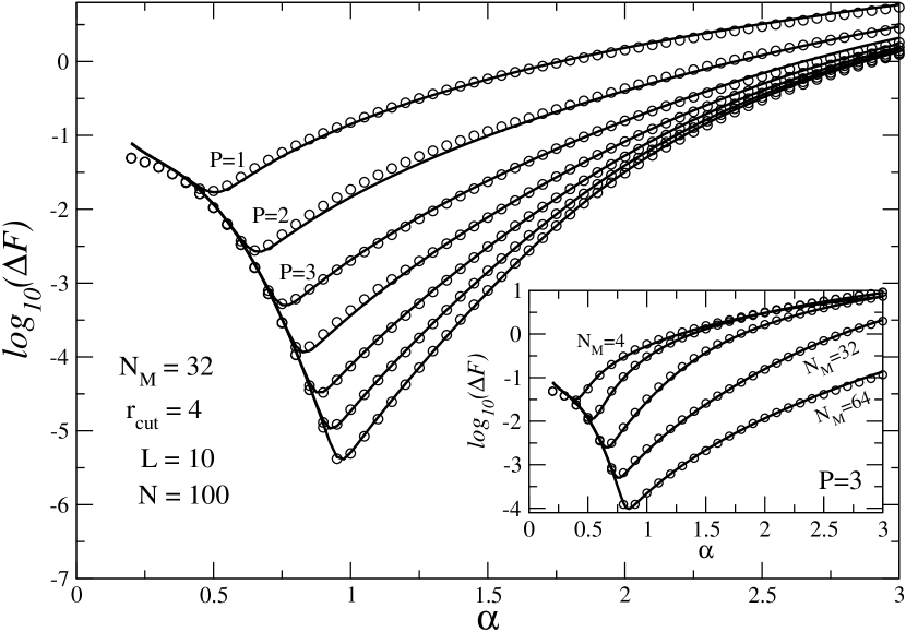
Figure 1: Figure 1

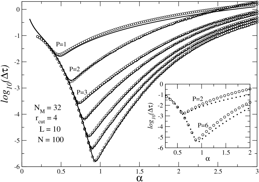
Figure 2: Figure 2

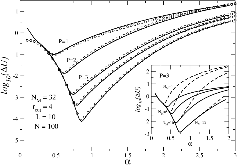
Figure 3: Figure 3

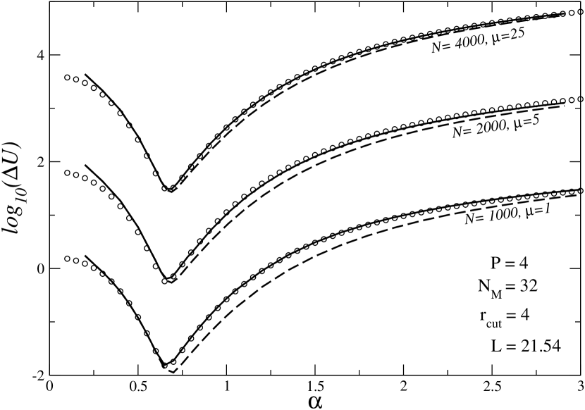
Figure 4: Figure 4

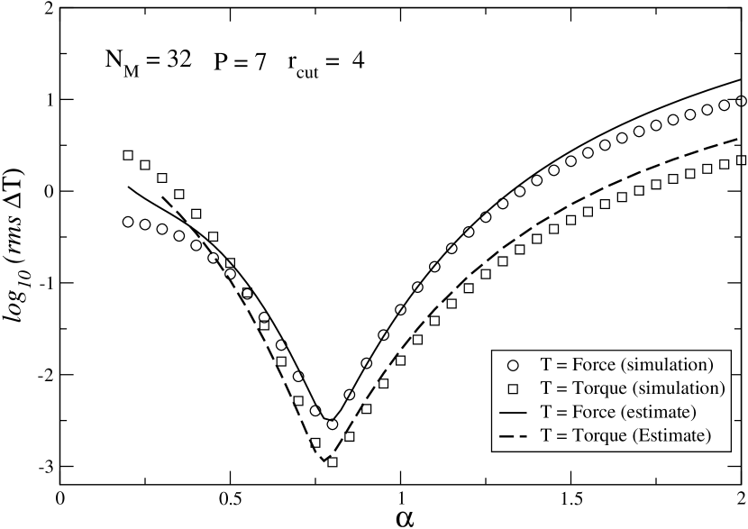
Figure 5: Figure 5

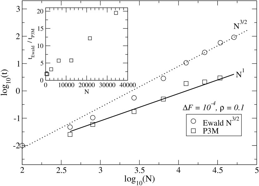
Figure 6: Figure 6

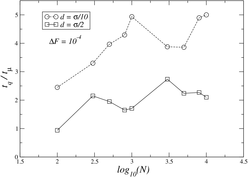
Figure 7: Figure 7

References

- (1) S. Odenbach, Magnetoviscous Effects in Ferrofluids, volume m71 of Lecture Notes in Physics, Springer, Berlin, Heidelberg, 2002.
- (2) R. E. Rosensweig, Ferrohydrodynamics, Cambridge Univ. Press, Cambridge, 1985.
- (3) B. M. Berkovsky, V. F. Medvedev, and M. S. Krakov, Magnetic Fluids, Engineering, Applications, Oxford University Press, Oxford, New York, Tokyo, 1993.
- (4) B. M. Berkovsky, editor, Magnetic Fluids and Applications Handbook, Begell House Inc., New York, 1996.
- (5) C. Holm and J.-J. Weis, Current Opinion in Colloid and Interface Science 10, 133 (2005).
- (6) J.-J. Weis and D. Levesque, Adv. Polym. Sci. 185, 163 (2005).
- (7) M. M. M. E. Blums, A. Cebers, Magnetic Fluids, Walter de Gruyter, 1997.
- (8) S. Odenbach and S. Thurm, Magnetoviscous effects in ferrofluids, in Ferrofluids: Magnetically Controllable Fluids and Their Applications, edited by S. Odenbach, volume 594 of Lecture Notes in Physics, pages 185–201, Springer, Berlin, Germany, 2002.
- (9) T. N. Heinz and P. H. Hünenberger, The Journal of Chemical Physics 123, 034107 (2005).
- (10) S. W. de Leeuw, J. W. Perram, and E. R. Smith, Proc. R. Soc. Lond. A 373, 27 (1980).
- (11) S. W. de Leeuw, J. W. Perram, and E. R. Smith, Proc. R. Soc. Lond. A 373, 57 (1980).
- (12) M. P. Allen and D. J. Tildesley, Computer Simulation of Liquids, Oxford Science Publications, Clarendon Press, Oxford, 1 edition, 1987.
- (13) Z. W. Wang and C. Holm, J. Chem. Phys. 115, 6277 (2001).
- (14) A. Toukmaji, C. Sagui, J. Board, and T. Darden, J. Chem. Phys. 113, 10913 (2000).
- (15) R. Kutteh and J. B. Nicholas, Computer Physics Communications 86, 236 (1995).
- (16) R. Kutteh and J. B. Nicholas, Computer Physics Communications 86, 227 (1995).
- (17) A. D. Stoycheva and S. J. Singer, Phys. Rev. E 65, 036706 (2002).
- (18) D. Christiansen, J. W. Perram, and H. G. Petersen, Journal of Computational Physics 107, 403 (1993).
- (19) A. Arnold and C. Holm, Efficient methods to compute long range interactions for soft matter systems, in Advanced Computer Simulation Approaches for Soft Matter Sciences II, edited by C. Holm and K. Kremer, volume II of Advances in Polymer Sciences, pages 59–109, Springer, Berlin, 2005.
- (20) J. Perram, H. Pedersen, and S. de Leeuw, J. Mol. Phys. 65, 875 (1988).
- (21) H. G. Petersen, The Journal of Chemical Physics 103, 3668 (1995).
- (22) C. Sagui and T. A. Darden, Annual Review of Biophysics and Biomolecular Structure 28, 155 (1999).
- (23) R. W. Hockney and J. W. Eastwood, Computer Simulations using Particles, McGraw-Hill, New York, 1981.
- (24) M. Deserno and C. Holm, J. Chem. Phys. 109, 7678 (1998).
- (25) C. Sagui and T. Darden, P3m and pme: a comparison of the two methods, in Simulation and Theory of Electrostatic Interactions in Solution, edited by L. Pratt and G. Hummer, page 104, 1999.
- (26) H. J. Limbach, A. Arnold, B. A. Mann, and C. Holm, Comput. Phys. Commun. 174, 704 (2006).
- (27) ESPResSo, Homepage, 2004, http://www.espresso.mpg.de.
- (28) P. Ewald, Ann. Phys. (Leipzig) 369, 253 (1921).
- (29) G. Rajagopal and R. Needs, J. Comput. Phys. 115, 399 (1994).
- (30) P. H. Hünenberger, The Journal of Chemical Physics 113, 10464 (2000).
- (31) P. F. Batcho and T. Schlick, The Journal of Chemical Physics 115, 8312 (2001).
- (32) D. Frenkel and B. Smit, Understanding Molecular Simulation, volume 1 of Computational Science Series, Academic Press, San Diego, 2 edition, 2002.
- (33) When meshes with number of points per direction are used to perform FFTs, the reciprocal mesh is asymmetric (the number of points along the positive axis, and the number along the negative axis differ by one). The use of asymmetric lattices, for instance, introduces systematic biases in the forces (see expression for the mean value of the forces in the reciprocal space, eq. (96)) which has to be corrected by adding extra terms. In this paper the results are derived assuming the use of symmetric lattices. We use meshes in which the reciprocal mesh has been symmetrized by disregarding the contributions from the -vector value without counterpart.
- (34) P. H. Hünenberger, The Journal of Chemical Physics 116, 6880 (2002).
- (35) V. Ballenegger, J. J. Cerda, O. Lenz, and C. Holm, J. Chem. Phys. 128, 034109 (2008).
- (36) Z. Wang, C. Holm, and H. W. Müller, Phys. Rev. E 66, 021405 (2002).
- (37) J. D. Weeks, D. Chandler, and H. C. Andersen, The Journal of Chemical Physics 54, 5237 (1971).
- (38) S. Kantorovich, J. J. Cerdà, and C. Holm, Phys. Chem. Chem. Phys 10, 1883 (2008).
- (39) J. J. Cerdà, S. Kantorovich, and C. Holm, Journal of Physics: Condensed Matter 20, 204125 (2008).
- (40) M. Deserno and C. Holm, J. Chem. Phys. 109, 7694 (1998).
- (41) The contribution to the (total) rms error arising from errors in MS energies is negligible only if the Ewald energy is corrected to compensate systematic cutoff errors in the MS energies of the particles. This correction, which is the analog of for standard Ewald sums, is termed the “diagonal” correction in refs. kolafa92a ; wang01a .
- (42) J. Kolafa and J. W. Perram, Molecular Simulation 9, 351 (1992).