LOLAS: an optical turbulence profiler in the atmospheric boundary layer with extreme altitude-resolution.

Abstract

We report the development and first results of an instrument called Low Layer Scidar (LOLAS) which is aimed at the measurement of optical-turbulence profiles in the atmospheric boundary layer with high altitude-resolution. The method is based on the Generalized Scidar (GS) concept, but unlike the GS instruments which need a 1-m or larger telescope, LOLAS is implemented on a dedicated 40-cm telescope, making it an independent instrument. The system is designed for widely separated double-star targets, which enables the high altitude-resolution. Using a $200^{\prime\prime}$-separation double-star, we have obtained turbulence profiles with unprecedented 12-m resolution. The system incorporates necessary novel algorithms for autoguiding, autofocus and image stabilisation. The results presented here were obtained at Mauna Kea Observatory. They show LOLAS capabilities but cannot be considered as representative of the site. A forthcoming paper will be devoted to the site characterisation. The instrument was built as part of the Ground Layer Turbulence Monitoring Campaign on Mauna Kea for Gemini Observatory.

1 Introduction

In recent years, a number of efforts have been conducted in the domain of astronomical adaptive optics to increase the field of view in which the wave front is corrected from atmospheric-turbulence-induced perturbations. Particularly, Ground Layer Adaptive Optics (GLAO) (Rigaut, 2002; Tokovinin, 2004) is aimed at compensating the wave front deformations arising from turbulence very close to the ground and not compensating those originating at higher altitudes. This idea is based on the facts that the compensation of lower altitude turbulent layers provides wider corrected fields of view (Chun, 1998) and that turbulence close to the ground is generally the most intense (e.g., Avila et al. (2004)).

To develop a GLAO system for a given site, it is required to have as much knowledge as possible about the optical turbulence in the ground layer (i.e. in the first kilometer of altitude above the site). For example, Le Louarn & Hubin (2006) recognize that the biggest unknown in their theoretical analysis of the performance of an infrared GLAO system is the vertical structure of the ground-layer turbulence ($C_{\mathrm{N}}^{2}(h)$) and that proper measurements are urgent to validate their results.

In view of such necessity, we have developed a method called Low Layer SCIDAR (LOLAS), the concept of which was presented by Avila & Chun (2004). It is based on the Generalised SCIDAR method (GS) but uses a smaller telescope and more widely separated double stars as targets. The method is explained in § 2. Egner & Masciadri (2007) reported the use of the GS technique to obtain $C_{\mathrm{N}}^{2}$ profiles measurements with an altitude resolution of a few tens of meters, which was the best GS resolution achieved so far. The fundamental difference of that work with the present one is that they use the 1.8-m Vatican Advanced Technology Telescope whereas we use a 40-cm dedicated telescope, which makes of LOLAS an independent monitor. See § 4 for further comments on the work by Egner & Masciadri (2007).

The experimental setup and data reduction for LOLAS is presented in § 3. The first results are shown in § 4 and finally, in § 5 we give the conclusion of this work.

2 LOLAS Concept

LOLAS is based on the GS concept (Avila et al., 1997; Fuchs et al., 1998), which consists of computing the normalised-mean spatial autocorrelation function of short exposure-time images of the scintillation pattern produced by a double star. The normalisation is performed with respect to the autocorrelation of the mean image. The resulting normalised autocorrelation map is dimensionally equivalent to a scintillation index, which is dimensionless. Hereafter, we will refer to this normalised-mean autocorrelation simply as the autocorrelation.

In the classical SCIDAR (Rocca et al., 1974; Caccia et al., 1987; Vernin, 1992), the analysis is made in the pupil plane of the telescope, which makes it insensitive to turbulence close to the ground because the scintillation variance is proportional to $h^{5/6}$ (Roddier, 1981), where $h$ is the altitude of the turbulent layer (acting as a phase screen). In the GS the plane of the detector is made the conjugate of a virtual plane (analysis plane) located at an altitude $h_{\mathrm{gs}}$ of the order of a few kilometers below the ground, hence $h_{\mathrm{gs}}<0$. In this case the distance relevant for scintillation produced by a turbulent layer at an altitude $h$ is $|\,h-h_{\mathrm{gs}}\,|$, which makes the turbulence at ground level detectable. Following Avila et al. (1997) and references therein, the autocorrelation function obtained can be written as

$$C_{\mathrm{gs}}\left(\mathbf{r}\right)=\int_{h_{\mathrm{gs}}}^{+\infty}{\rm d}h\;K\left(\mathbf{r},h-h_{\mathrm{gs}}\right)\;C_{N}^{2}\left(h\right)+N(\mathbf{r})\mbox{,}$$ (1)

where the kernel $K\left(\mathbf{r},h-h_{\mathrm{gs}}\right)$ is the theoretical autocorrelation function produced by a single layer at an altitude $h$ with a unit $C_{N}^{2}$ and $N(\mathbf{r})$ is the measurement noise. When $h<0$, $C_{\mathrm{N}}^{2}(h)$=0. For a double star of angular separation $\boldsymbol{\rho}$, the Kernel consists of three autocorrelation peaks: one centered on the autocorrelation origin and the two others separated from the first one by $\mathbf{d}_{\mathrm{r}}=\boldsymbol{\rho}|h-h_{\mathrm{gs}}|$ and $\mathbf{d}_{\mathrm{l}}=-\boldsymbol{\rho}|h-h_{\mathrm{gs}}|$. The altitude of the layer is determined from the measurement of $\mathbf{d}_{\mathrm{r}}$ or $\mathbf{d}_{\mathrm{l}}$ and the solution of the corresponding equation.

The altitude resolution is equal to $\Delta d/\rho$, where $\Delta d$ is the minimal measurable difference of the position of two autocorrelation peaks. The natural value of $\Delta d$ is the full width at half maximum $L$ of the aucorrelation peaks: $L(h)=0.78\sqrt{\lambda(h-h_{\mathrm{gs}})}$ (Prieur et al., 2001), where $\lambda$ is the wavelength. However, $\Delta d$ can be shorter than $L$ if the inversion of Eq. 1 is performed using a method that can achieve super-resolution like Maximum Entropy or CLEAN. Both methods have been used in GS measurements (Prieur et al., 2001). Fried (1995) analised the CLEAN algorithm and its implications for super-resolution. Applying his results for GS leads to an altitude resolution of

$$\Delta h=\frac{2}{3}\frac{L}{\rho}=0.52\frac{\sqrt{\lambda(h-h_{\mathrm{gs}})}}{\rho}.$$ (2)

The maximum altitude, $h_{\mathrm{max}}$ for which the $C_{\mathrm{N}}^{2}$ value can be retrieved is set by the altitude at which the projections of the pupil along the direction of each star cease to be overlapped, as no correlated speckles would lie on the scintillation images coming from each star. Figure  1 illustrates the basic geometrical consideration involved in the determination of $h_{\mathrm{max}}$ . Note that $h_{\mathrm{max}}$ does not depend on $h_{\mathrm{gs}}$. The maximum altitude is thus given by

$$h_{\mathrm{max}}=\frac{D}{\rho},$$ (3)

where $D$ is the pupil diameter.

In addition to the autocorrelation of the scintillation images, the GS calculates the mean cross-correlation of images taken at times separated by a known constant delay $\Delta t$. As explained by Avila et al. (2001); Prieur et al. (2004); Avila et al. (2006), the cross-correlation leads to the determination of the velocity of the turbulent layers and the $C_{\mathrm{N}}^{2}$ of the turbulence generated inside the telescope dome.

LOLAS concept consists of the implementation of the GS technique on a small dedicated telescope, using a very widely separated double star. For example, for $h_{\mathrm{gs}}=-2$ km, $h=0$, $\lambda=0.5$ $\mu$m, $D=40$ cm and star separations of 180^′′ and 70^′′, $\Delta h$ equals 19 and 48 m, while $h_{\mathrm{max}}$ equals 458 and 1179 m, respectively. GS uses a larger telescope (at least 1-m diameter) and closer double stars, so that the entire altitude-range with non-negligible $C_{\mathrm{N}}^{2}$ values is covered ($h_{\mathrm{max}}\gtrsim 30$ km).

The altitude of the analysis plane, $h_{\mathrm{gs}}$ was set to -2 km, as a result of a compromise between the increase of scintillation variance, which is proportional to $|h-h_{\mathrm{gs}}|^{5/6}$, and the reduction of pupil diffraction effects. Indeed, pupil diffraction caused by the virtual distance between the pupil and the analysis planes provokes that Eq. 1 is only an approximation. The larger $h_{\mathrm{gs}}$ or the smaller the pupil diameter, the greater the error in applying Eq. 1. We have performed numerical simulations to estimate such effect. A succinct description of the simulations is presented in Appendix A.

The pixel size projected on the pupil, $d_{\mathrm{p}}$, is set by the condition that the smallest scintillation speckles be sampled at the Nyquist spatial frequency or better. The typical size of those speckles is equal to $L(0)$. Taking the same values as above for $h_{\mathrm{gs}}$ and $\lambda$, yields $L(0)=2.45$ cm. We chose $d_{\mathrm{p}}=1$ cm, which indeed satisfies the Nyquist criterion $d_{\mathrm{p}}\leq L(0)/2$. The altitude sampling of the turbulence profiles is $\delta_{h}=d_{p}/\rho$. Note, from the two last expressions and Eq. 2, that the altitude resolution $\Delta h$ and the altitude sampling $\delta_{h}$ are related by $\delta_{h}\leq(3/4)\Delta h$ for $h=0$.

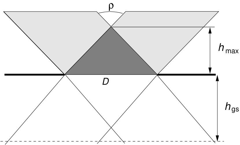
[t]

Figure 1: Schematic for the determination of the maximum altitude $h_{\mathrm{max}}$ for which the $C_{\mathrm{N}}^{2}$ value can be retrieved. The altitude of the analysis plane $h_{\mathrm{gs}}$ is represented only to make clear that this value is not involved in the calculation of $h_{\mathrm{max}}$.

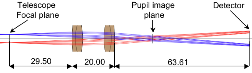
Figure 2: Optical layout. The dimensions unit is millimeters.

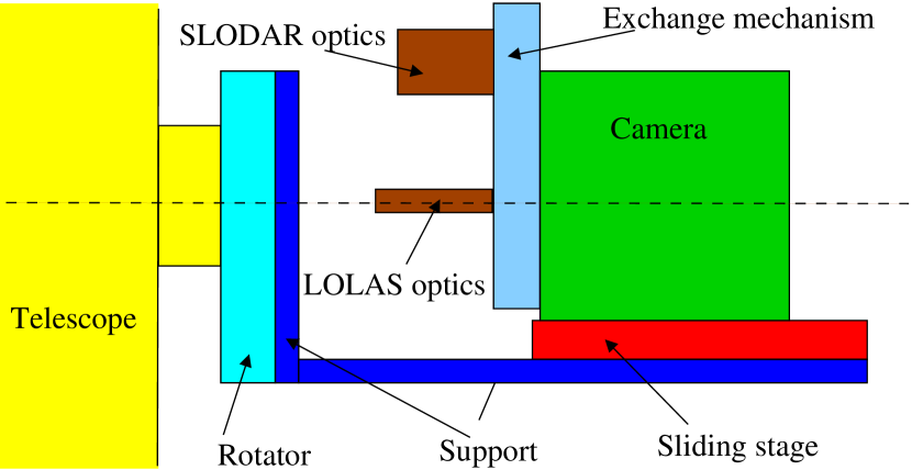
Figure 3: Schematic view of the instrument. The drawing is not on scale.

3 Instrument

3.1 Hardware

A 40-cm Meade telescope installed on an equatorial mount sends light to a pair of 50-mm focal-length achromatic lenses that form on the detector an image of a virtual plane located approximately 2 km below the pupil. Figure 2 represents a scaled optical layout showing the optical beams of two stars separated by 200^′′ as they travel from the telescope focal plane to the detector. The beam sizes correspond to the telescope-pupil diameter. The diameter of each beam at the detector plane is equal to 1.30 mm. In some GS systems a field lens is used to shift the image of the analysis plane either further away from the telescope focus or closer to it, whether the lens is diverging or converging, respectively. The optical setup for LOLAS was designed so to avoid the use of a field lens. The detector is an Electron Multiplying Charged Couple Device (EMCCD) manufactured by Andor Technology with 512$\times$512 square pixels of 16 $\mu$m side each. The maker asserts that the effective readout noise is smaller than 1 electron r.m.s. and the quantum efficiency is higher than 90%. Frames are binned 2$\times$2. The size of each binned pixel on the conjugated plane is 9.8 mm. One can chose any size for the active sub-array of the detector to be red. Figure 3 shows a schematic view of the instrument. The telescope holds a motrised rotator used to align the pixel lines along the separation of the double star. The rotator holds the mechanical support that carries the rest of the instrument. A sliding stage, which enables precise positioning along the optical axis, is screwed on the support and carries the camera. The same equipment, except for the optics, is used for Slope Detection and Ranging (SLODAR) observations. The SLODAR (Wilson et al., 2004; Butterley et al., 2006) exploits Shack-Hartmann wavefront sensor measurements of the slope of the phase aberration produced by the atmospheric turbulence. This technique is implemented by replacing LOLAS focusing optics by a collimator and a lenslet array. To easily switch between LOLAS and SLODAR configurations, a manual mechanism is attached to the camera and holds the optics of the two experiments. The mechanism is designed to ensure the correct position of each optical assembly. Figure 3 shows the LOLAS optics barrel in place. Into this barrel the LOLAS focusing lenses are mounted. The telescope, camera, stage and rotator are controlled by a Personal Computer (PC) with two 3-GHz Xeon processors and 1-GB memory capacity, running under Linux operating system.

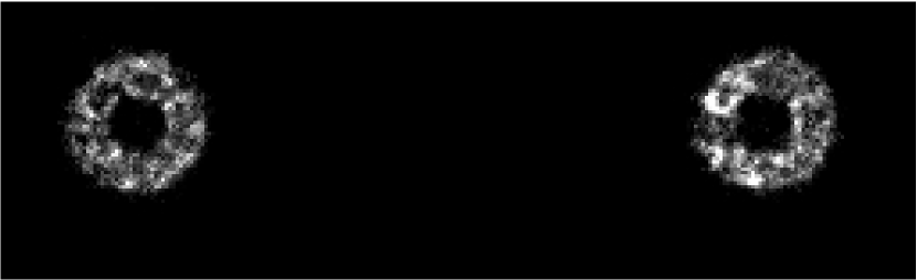
[t]

Figure 4: Example of a scintillation image acquired with LOLAS. The exposure time was set to 3 ms. The analysis plane is located at $h_{\mathrm{gs}}=-2$ km. The object is the double star “STF 4” of coordinates $\alpha_{2000}=01\mathrm{h}\;56\hbox to0.0pt{.\hss}^{\prime}2$ and $\delta_{2000}=+37^{\circ}\;15^{\prime}$. The V-magnitudes of the stars are 5.68, 6.10 and their separation is $199\hbox to0.0pt{.\hss}^{\prime\prime}7$.

3.2 Data acquisition and processing

The out-of-focus pupil images produced by each star are centered on the detector. To optimize the acquisition and processing speed, only a sub-frame of 256$\times$80 binned pixels is acquired. An example is shown in Fig. 4. The exposure time of each frame ranges from 3 to 10 ms, depending on the wind conditions, and is selected by the user. The typical number of frames used to obtain one set of auto- and cross-correlations is 30000. The frame rate at 3 ms exposure time is 112 frames per second.

In windy conditions, telescope shaking can cause image motion which affects the calculation of the mean image. To avoid this, every image is recentered prior to co-addition of the frames. In addition, telescope tracking errors are corrected by updating the telescope position every 200 images, using the average image position of the most recently acquired 200-frames packet. This autoguiding keeps the extra-pupil images on the active sub-array of the detector. It has been seen that the pupil images slowly change in size. This is due to a slow shift of the telescope focus, presumably caused by the redistribution of the primary mirror load while tracking the stars. An autofocus system has been developed to overcome this problem. On every average image calculated with 200 frames, the size of the out-of-focus pupils is monitored and the camera and optics are moved by acting on the supporting sliding stage, until the nominal size of 40 binned pixels is recovered. Similarly, the alignment of the stars along the pixel lines is measured and eventually corrected automatically by acting on the motorised rotator. Finally, the average flux over the pupil is also monitored in each image and its variance relative to the mean flux is calculated and stored in the header of the FITS file in which the correlations are saved. This information is used to qualify the data. Indeed, mean flux variations, due to cloud passages or fog condensation, are adverse to the retrieval of $C_{\mathrm{N}}^{2}$ profiles from the autocorrelations.

The auto- and cross- correlations are calculated as images are being acquired. When a set of correlations are saved on disk, an IDL program is automatically executed to invert Eq. 1 and retrieve $C_{\mathrm{N}}^{2}(h)$, using a modified CLEAN algorithm similar to that developed by Prieur et al. (2001) for GS measurements.

4 First results

The first results of LOLAS as described in § 3 were obtained in September 2007 at Mauna Kea Observatory, as part of a collaboration between the Universidad Nacional Autónoma de México (UNAM), the University of Durham (UD) and the University of Hawaii (UH), under a contract with Gemini Observatory. The instrument was installed on the Coudé roof of the UH 2.2-m telescope.

Figure 5 shows an example of the autocorrelation map of scintillation images obtained with the double star “STF 28” of angular separation of $\rho=108\hbox to0.0pt{.\hss}^{\prime\prime}4$, which is considered a moderate separation for LOLAS. The number of frames used for this example was 30000 and the exposure time of each frame was 3 ms. The central peak is the result of the summation of the central peaks produced by all the turbulent layers in the atmosphere, even those that are higher than the maximum altitude $h_{\mathrm{max}}$ reached by the instrument, which in this case is equal to 764 m (Eq. 3). The correlated speckles produced by those layers are separated by a longer distance than the pupil diameter, thereby not giving rise to lateral peaks inside the autocorrelation-map bounds. Only the layers below $h_{\mathrm{max}}$ form visible lateral peaks from which $C_{\mathrm{N}}^{2}(h)$ is retrieved. The right-hand-side wing of those peaks in Fig. 5 are framed by rectangle A. The most intense peak inside that frame corresponds to the ground level and is a consequence of the turbulence inside and outside the telescope tube. Much fainter peaks further apart from the map center - thus from higher layers - can be seen inside frame A. It is worth noting that the color scale for that figure was chosen such that the fainter peaks are visible, not caring if the stronger peaks appear saturated. The autocorrelation signal is contained inside a strip which is vertically centered and aligned along the horizontal axis, because the detector pixels were aligned along the direction of the double-star separation. Hence, the values inside frame B correspond only to noise. The standard deviation $\sigma_{\mathrm{ac}}$ of those values is used as a measure of the noise level in the data. In this case, $\sigma_{\mathrm{ac}}=4.5\times 10^{-4}$. Following Roddier (1981), the relation between $C_{\mathrm{N}}^{2}$(0) and a scintillation variance $\sigma_{\mathrm{I}}$ is:

$$C_{\mathrm{N}}^{2}(0)=\frac{\sigma_{\mathrm{I}}\lambda^{7/6}|h_{\mathrm{gs}}|^{-5/6}}{19.12\;\delta_{h}}.$$ (4)

For the data shown in Fig 5, $\delta_{h}=19$ m, hence $\sigma_{\mathrm{ac}}$ corresponds to a $C_{\mathrm{N}}^{2}$ uncertainty of $\Delta C_{\mathrm{N}}^{2}=1\times 10^{-16}$ m^-2/3. Correlation values larger than $3\sigma_{\mathrm{ac}}$ are considered as being actual signal. This sets the minimum detectable $C_{\mathrm{N}}^{2}$ value to $C_{\mathrm{N_{min}}}^{2}=3\times 10^{-16}$ $\mathrm{m}^{-2/3}$. Note that $\Delta h$ is defined as the resolution along the line-of-sight. For this case, $\Delta h=31$ m, for h=0. The altitude resolution at ground level in the vertical direction is $\Delta h\cos(z)$, where $z$ is the zenith angle. In this case $z=35.6^{\circ}$ which results in a vertical resolution of 25.4 m. The $C_{\mathrm{N}}^{2}$ profile corresponding to that autocorrelation is shown in Fig. 6. The contribution of turbulence inside the telescope tube has been removed from the $C_{\mathrm{N}}^{2}$ value at ground level. To do so, we used the temporal cross-correlation of images taken with a temporal interval of 13 ms (26 or 39 ms can also be chosen, depending on local wind speed), calculated with the same data as that used for the autocorrelation of Fig. 5. This cross-correlation is shown in Fig. 7. The correlation triplet that is centered on the cross-correlation origin is interpreted as arising from static turbulence inside the telescope tube (see Avila et al. (2001) for details of that method). The corresponding value of the $C_{\mathrm{N}}^{2}$ is 8.9$\times 10^{-15}$ $\mathrm{m}^{-2/3}$, which is equivalent to $0\hbox to0.0pt{.\hss}^{\prime\prime}37$ seeing.

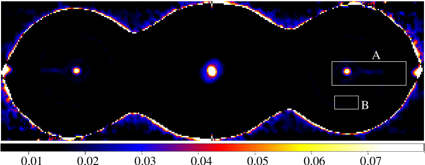
Figure 5: Example of an autocorrelation obtained with a moderately separated star ($\rho=108\hbox to0.0pt{.\hss}^{\prime\prime}4$). The scale is indicated by the false-color code at the bottom. As explained in  § 2 the autocorrelations are dimensionless.

Figure 6: Examples of $C_{\mathrm{N}}^{2}$ profiles. LOLAS profile was obtained from the autocorrelation shown in Fig. 5, in 2007 July 3 at 9:51 UT. The SLODAR profile was obtained the same date at 10:19 UT. $C_{\mathrm{N}}^{2}$ uncertainties for LOLAS and SLODAR are $\pm 1\times 10^{-16}$ and $\pm 3\times 10^{-16}$ m^-2/3.

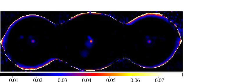
Figure 7: Cross correlation obtained with the same data as the autocorrelation shown in Fig. 5.

In Fig. 6 is also shown a $C_{\mathrm{N}}^{2}$ profile measured with the SLODAR, 28 minutes later than the measurement done with LOLAS, using the same stellar source. The $C_{\mathrm{N}}^{2}$ uncertainty is obtained using the bootstrap method. The altitude resolution achievable with LOLAS is approximately 5 times better than that for SLODAR. This is clearly illustrated by the profiles shown in Fig. 6: Around 200 m, LOLAS separates two layers, centered at 150 and 210 m, while the SLODAR delivers a single $C_{\mathrm{N}}^{2}$ peak centered at 190 m, approximately. Similarly, in the 70 m, LOLAS identifies two layers while the SLODAR only one. Note that the sum of the $C_{\mathrm{N}}^{2}$ values delivered by LOLAS in the latter altitude range agrees with the SLODAR value at ground level within 10%. Both measurements are free of the effect of the turbulence inside the telescope tube. The lower altitude resolution of SLODAR is related to a wider spatial sampling on the analysis plane. Here we used an array of $8\times 8$ sub-apertures, each of diameter 5 cm, which is five times larger than $d_{p}$. This implies that the photon flux per spatial resolution element and hence the instantaneous signal-to-noise ratio of LOLAS measurements is five times lower than for the SLODARs, so that a five times longer period of integration is required to measure the turbulence profile to a given accuracy. Hence in practice a choice can be made between greater altitude resolution (LOLAS) or greater temporal resolution (SLODAR) of the profile.

To illustrate the highest altitude resolution that has so far been reached with LOLAS, Fig. 8 shows a $C_{\mathrm{N}}^{2}$ profile obtained using as target a $199\hbox to0.0pt{.\hss}^{\prime\prime}7$-separation double-star. The altitude resolution in vertical direction is 11.7 m and $\Delta C_{\mathrm{N}}^{2}=1.6\times 10^{-16}\mathrm{m}^{-2/3}$. Note the ability for discerning a layer centered at 16 m from that at ground layer. Similarly to the profile shown in Fig. 6, the turbulence inside the telescope tube has been removed. To make certain that the $C_{\mathrm{N}}^{2}$ peak at 16 m is not an artifact produced by the inversion algorithm, Fig. 9 shows the corresponding auto- and cross- correlations. Only an enlargement of the central and right-hand-side peaks is shown. In the autocorrelation, the right-hand side peak appears slightly elongated in the horizontal direction, suggesting that this peak is in fact the result of two layers very close to each other. This is confirmed on the cross-correlation map, where one can clearly see the contribution of two distinct layers: peaks 1 correspond to the ground layer and peaks 2 come from a slightly higher layer as the separation of the latter peaks is larger than that of peaks 1. The altitude resolution might be improved if the information contained in the cross-correlation map was systematically used (Egner & Masciadri, 2007).

Figure 8: Example of a turbulence profile with the highest altitude-resolution so far obtained with LOLAS. The data was taken in 2007 November 17 at 12:09 UT. The central frame shows an amplification of the profile in the low-altitude zone. The $C_{\mathrm{N}}^{2}$ uncertainty is $\pm 1.6\times 10^{-16}$ m^-2/3.

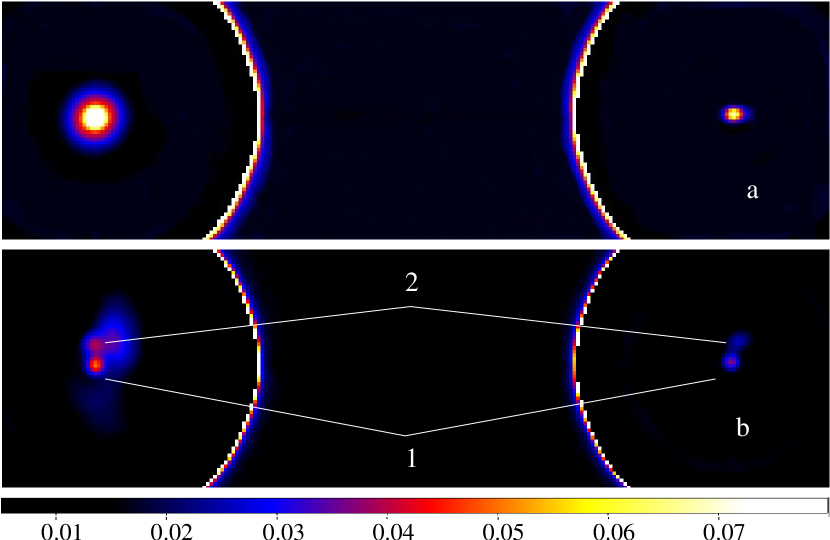
Figure 9: Similar to Figs. 5 (for a) and 7 (for b), but obtained with a widely separated double star ($\rho=199\hbox to0.0pt{.\hss}^{\prime\prime}7$).

5 Conclusions

An instrument has been created for the monitoring of optical turbulence profiles in the atmospheric boundary layer with an altitude resolution that can reach 11.7 m. It is a stand-alone system that needs only an external power supply, making it a suitable device for long-term monitoring at developed and undeveloped astronomical sites. The system incorporates algorithms that automatically preserve the correct image position on the detector, focus and camera rotational position. Temporal variations of the pupil-averaged flux are also calculated automatically and stored in the output files as auxiliary data for data reduction. The computation of the auto- and cross- correlation is performed in real time and the $C_{\mathrm{N}}^{2}$ profile is automatically retrieved immediately after the correlations are stored on disk. Numerical simulations of the effect of pupil diffraction show that it reduces the values of the autocorrelation by 10%. Nevertheless, this alteration is corrected before applying the inversion algorithm. The turbulence originated inside the telescope tube can be removed from the $C_{\mathrm{N}}^{2}$ profile on a post-processing step. The first results have shown the very high capabilities of LOLAS in terms of altitude resolution. The shortest vertical resolution is only twice that of the instrumented balloons, which is of the order of 6 m (Azouit & Vernin, 2005). One disadvantage of LOLAS compared to the balloons, SLODAR, GS, Multi-Aperture Scintillation Sensor (MASS) (Kornilov et al., 2003) or Single Star Scidar (SSS) (Habbib et al., 2006) is that until now it does not provide $C_{\mathrm{N}}^{2}$ values of the free atmosphere. However, scintillation generated at higher layers is indeed detected with LOLAS. This information could be used in two possible ways: performing a post-detection spatial filtering using MASS-like masks or using SSS-like algorithms to retrieve $C_{\mathrm{N}}^{2}$values from the central peaks of cross-correlations obtained with a set of different temporal intervals. SLODAR is the remote-sensing technique that has a vertical resolution closer to that of LOLAS. The advantage of SLODAR over LOLAS is that the temporal resolution of the $C_{\mathrm{N}}^{2}(h)$ measurements is five times higher. A first comparison of the profiles delivered by LOLAS and SLODAR have shown a fairly good agreement between both techniques, although a more thorough comparative study needs to be done to draw a definitive conclusion. The turbulence profiles shown here are not to be taken as representative of the site. A proper monitoring campaign at Mauna Kea is currently being carried out and a statistical analysis of the results will be the subject of a forthcoming paper.

Appendix A Pupil diffraction effect

The effect of pupil diffraction has been investigated by numerical simulations of the normalised autocorrelation of scintillation images of a double star, on a 40-cm telescope. There is no analytical investigation of this effect in the literature. We used the SCIDAR Simulator (Cruz et al., 2003) which is based on the optical turbulence simulator named Turbulenz.

Plane waves coming from two stars separated by 1 arc-minute pass through three turbulent layers located at altitudes $h$ of 100, 300 and 700 m above the ground. The three layers have equal $C_{\mathrm{N}}^{2}$ corresponding to a Fried parameter of 20 cm. The phase of the waves are distorted by the turbulent layers following a Kolmogorov spectrum. Between the layers and down to the simulated detection plane, wave propagation is taken into account by calculating Fresnel diffraction of the complex amplitudes. At ground level, a mask is applied to the complex amplitudes, which simulates an unaberrated pupil of a 40-cm Meade telescope, including the central obscuration. The intensity of the resulting waves are calculated on the detection plane, located 2 km below the ground (i.e. $h_{\mathrm{gs}}=-2$ km). The autocorrelation of the intensity map is calculated and co-added for 1000 statistically independent samples. This co-added autocorrelation is normalized by the autocorrelation of the mean intensity. The amplitude and shape of the correlation peaks obtained for the corresponding layers are compared to the theoretical ones that would be obtained with an infinite pupil-size. Those theoretical values are calculated by considering that the correlation amplitude is proportional to $C_{\mathrm{N}}^{2}h^{5/6}$ and the width of the correlation peak is proportional to $\sqrt{\lambda L}$. The amplitude of the simulated correlation peaks are 3.4%, 8.4% and 9.3% smaller than the amplitudes of the theoretical peaks, for the layers at 100, 300 and 700 m, respectively. The measured autocorrelation peaks are corrected by a factor obtained by the interpolation of those factors for the altitude of the corresponding layer, before applying the inversion procedure which is designed for an infinite pupil-size.

References

- Avila et al. (2006) Avila R., Carrasco E., Ibañez F., Vernin J., Cruz D., 2006, PASP, 118, 503
- Avila & Chun (2004) Avila R., Chun M., 2004, in Bonnaccini D., Ellerbroek B., Raggazzoni R., eds, Advancements in Adaptive Optics Vol. 5490, A method for high altitude resolution profiling in the first few hundred meters. pp 742–748
- Avila et al. (2004) Avila R., Masciadri E., Vernin J., Sánchez L., 2004, PASP, 116, 682
- Avila et al. (1997) Avila R., Vernin J., Masciadri E., 1997, Appl. Opt., 36, 7898
- Avila et al. (2001) Avila R., Vernin J., Sánchez L. J., 2001, A&A, 369, 364
- Azouit & Vernin (2005) Azouit M., Vernin J., 2005, PASP, 117, 536
- Butterley et al. (2006) Butterley T., Wilson R. W., Sarazin M., 2006, 369, 835
- Caccia et al. (1987) Caccia J. L., Azouit M., Vernin J., 1987, Appl. Opt., 26, 1288
- Chun (1998) Chun M., 1998, PASP, 110, 317
- Cruz et al. (2003) Cruz D. X., González S. I., Angeles F., Avila R., Sánchez L. J., Iriarte A., Cuevas S., Martínez L. A., Farah A., Sánchez B., Martínez M., 2003, in Cruz-González I., Avila R., Tapia M., eds, San Pedro Mártir: Astronomical Site Evaluation Vol. 19, Development of a generalized scidar at unam. Revista Mexicana de Astronomía y Astrofísica (serie de conferencias), pp 44–51
- Egner & Masciadri (2007) Egner S. E., Masciadri E., 2007, PASP, 119, 1441
- Fried (1995) Fried D. L., 1995, J. Opt. Soc. Am. A, 12, 853
- Fuchs et al. (1998) Fuchs A., Tallon M., Vernin J., 1998, PASP, 110, 86
- Habbib et al. (2006) Habbib A., Vernin J., Benkhaldoun Z., Lanteri H., 2006, MNRAS, 368, 1456
- Kornilov et al. (2003) Kornilov V., A.Tokovinin Vozyakova O., A. Shatsky N., S. S. P., Sarazin M., 2003, in Wizinowich P., Bonnaccini D., eds, Adaptive Optical System Technologies II Vol. 4839, Mass: a monitor of the vertical turbulence distribution. pp 837–845
- Le Louarn & Hubin (2006) Le Louarn M., Hubin N., 2006, MNRAS, 365, 1324
- Prieur et al. (2004) Prieur J. L., Avila R., Daigne G., Vernin J., 2004, PASP, 116, 778
- Prieur et al. (2001) Prieur J.-L., Daigne G., Avila R., 2001, A&A, 371, 366
- Rigaut (2002) Rigaut F., 2002, in Vernet E., Ragazzoni R., Esposito S., Hubin N., eds, Beyond conventional adaptive optics Vol. 58, 3d optical turbulence characterization for the new class of adaptive optics techniques. ESO Conference and Workshop Proceedings, pp 11–16
- Rocca et al. (1974) Rocca A., Roddier F., Vernin J., 1974, J. Opt. Soc. Am. A, 64, 1000
- Roddier (1981) Roddier F., 1981, Progress in Optics, XIX, 281
- Tokovinin (2004) Tokovinin A., 2004, PASP, 116, 941
- Vernin (1992) Vernin J., 1992, in Tatarskii V. I., Ishimaru A., Zavorotny V. U., eds, Wave propagation in Random Media (Scintillation) - Invited papers Atmospheric turbulence profiles. SPIE Press, Bellingham, Wash., pp 248–260
- Wilson et al. (2004) Wilson R. W., Bate J., Guerra J. C., Sarazin M., Saunter C., 2004, in Bonnaccini D., Ellerbroek B., Raggazzoni R., eds, Advancements in Adaptive Optics Vol. 5490, Development of a portable slodar turbulence profiler. pp 758–765