Empirical analysis of the worldwide maritime transportation network

Abstract

In this paper we present an empirical study of the worldwide maritime transportation network (WMN) in which the nodes are ports and links are container liners connecting the ports. Using the different representations of network topology namely the space $L$ and $P$, we study the statistical properties of WMN including degree distribution, degree correlations, weight distribution, strength distribution, average shortest path length, line length distribution and centrality measures. We find that WMN is a small-world network with power law behavior. Important nodes are identified based on different centrality measures. Through analyzing weighted cluster coefficient and weighted average nearest neighbors degree, we reveal the hierarchy structure and rich-club phenomenon in the network.

I Introduction

The recent few years have witnessed a great devotion to exploration and understanding of underlying mechanism of complex systems as diverse as the Internet Barabasi , social networks Newman1 and biological networks Jeong . As critical infrastructure, transportation networks are widely studied. Examples include airline Amaral ; GuimeraPNAS ; Wli ; chiliping ; Guida , ship Xinping1 , bus Sienkiewicz ; Xinping2 ; liping ; Ferber , subway Latorasubway and railway Sen ; wli2 networks.

Maritime transportation plays an important role in the world merchandize trade and economics development. Most of the large volume cargo between countries like crude oil, iron ore, grain, and lumber are carried by ocean vessels. According to the statistics from United Nations maritimereport , the international seaborne trade continuously increased to 7.4 billion tons in 2006 with a robust annual growth rate of $4.3$ per cent. And over 70 per cent of the value of world international seaborne trade is being moved in containers.

Container liners have become the primary transportation mode in maritime transport since 1950’s. Liner shipping means the container vessels travel along regular routes with fixed rates according to regular schedules. At present most of the shipping companies adopt hub-and-spoke operating structure which consists of hub ports, lateral ports, main lines and branch lines, forming a complex container transportation network system Rodrigue .

Compared with other transportation networks, the maritime container liner networks have some distinct features: (1) A great number of the routes of container liners are circular. Container ships call at a series of ports and return to the origin port without revisiting each intermediate port. It’s called pendulum service in container transportation. While bus transport networks and railway networks are at the opposite with most of buses or trains running bidirectionally on routes. (2) The network is directed and asymmetric due to circular routes. (3) Lines are divided into main lines and branch lines. Main lines are long haul lines which involves a set of sequential port calls across the oceans. Sometimes long haul lines call at almost 30 ports. Branch lines are short haul lines connecting several ports in one region to serve for main lines.

We construct the worldwide maritime transportation network (WMN) using two different network representations and analyze basic topological properties. Our result shows that the degree distribution follows a truncated power-law distribution in the space $L$ and an exponential decay distribution in the space $P$. With small average shortest path length 2.66 and high cluster coefficient 0.7 in the space $P$, we claim that WMN is a small world network. We also check the weighted network and find the network has hierarchy structure and "rich-club" phenomenon. Centrality measures are found to have strong correlations with each other.

The rest of the paper is organized as follows: in Section II, we introduce the database and set up the network using two different network representations. In Section III various topological properties are studied including degree distribution, degree correlations, shortest path length, weight distribution and strength distribution etc. Section IV discloses the hierarchy structure by studying the weighted and unweighted clustering and degree correlations. Centrality measures correlations and central nodes’ geographical distribution are studied in Section V. Section VI gives the conclusion.

II Construction of the network

We get the original data from a maritime transport business database named CI-online CIonline which provides ports and fleet statistics of 434 ship companies in the world. The data includes 878 sea ports and 1802 lines. The ports are distributed in different regions and we list the number of ports in each region in Table 1.

Table 1: Number of sea ports by major geographic region

Region			No of sea ports
Africa			96
Asia and Middle East			251
Europe			311
North America			61
Latin America			96
Oceania			63
Total			878

Figure 1: Description of the space $L$ and the space $P$. (a) and (b) are the undirected representations in the space $L$ and the space $P$ respectively. (c) and (d) are the directed representations in the space $L$ and the space $P$ respectively. In the space $L$, a link is created between consecutive stops in one route. In the space $P$ all ports that belong to the same route are connected. Line A (solid line) and line B (dashed line) are two different pendulum routes sharing one common node: the port No. 1.

To construct the worldwide maritime transportation network, we have to introduce the concept of spaces $L$ and $P$ as presented in Fig. 1. The idea of spaces $L$ and $P$ is first proposed in a general form in Sen and later widely used in the study of public bus transportation networks and railway networks. The space $L$ consists of nodes being ports and links created between consecutive stops in one route. Degree $k$ in the space $L$ represents the number of directions passengers or cargoes can travel at a given port. The shortest path length in the space $L$ is the number of stops one has to pass to travel between any two ports. In the space $P$, two arbitrary ports are connected if there is a container line traveling between both ports. Therefore degree $k$ in the space $P$ is the number of nodes which can be reached without changing the line. The shortest path length between any two nodes in the space $P$ represents the transfer time plus one from one node to another and thus is shorter than that in the space $L$.

Since WMN is a directed network, we extend the concept of spaces $L$ and $P$ to directed networks according to Xinping1 . See Fig. 1. Line A and B are two different pendulum routes crossing at the port No. 1. (a) and (b) is the undirected network representation. (c) and (d) is the respective directed version.

Based on the above concepts we establish the network under two spaces represented by asymmetrical adjacent matrices $A^{L}$, $A^{P}$ and weight matrices $W^{L}$, $W^{P}$. The element $a_{ij}$ of the adjacent matrix $A$ equals to 1 if there is a link from node $i$ to $j$ or 0 otherwise. The element $w_{ij}$ of weight matrix $W$ is the number of container lines traveling from port $i$ to port $j$.

We need to define the quantities used in this weighed and directed network. We employ $k^{L}_{in}(i)$ and $k^{L}_{out}(i)$ to denote in-degree, out-degree of node $i$ in the space $L$, and $k^{L}_{un}(i)$ to represent undirected degree in the space $L$. Similarly $k^{P}_{in}(i)$, $k^{P}_{out}(i)$ and $k^{P}_{un}(i)$ are employed in the space $P$. Hence we have

$$k^{L}_{in}(i)=\sum_{j\neq i}a_{ji}^{L}$$ (1)

$$k^{L}_{out}(i)=\sum_{j\neq i}a_{ij}^{L}$$ (2)

$$k^{L}_{un}(i)=\sum_{j\neq i}(a_{ij}^{L}+a_{ji}^{L})$$ (3)

which also holds for the space $P$.

Strength is also divided into in-strength and out-strength. In the space $L$ the in-strength of node $i$ is denoted by $S^{L}_{in}(i)$ and out-strength is denoted by $S^{L}_{out}(i)$. Undirected strength (total strength) is represented by $S^{L}_{un}(i)$. They can be calculated according to the following equations:

$$S^{L}_{in}(i)=\sum_{j\neq i}w_{ji}^{L}$$ (4)

$$S^{L}_{out}(i)=\sum_{j\neq i}w_{ij}^{L}$$ (5)

$$S^{L}_{un}(i)=\sum_{j\neq i}(w_{ij}^{L}+w_{ji}^{L})$$ (6)

which also holds for $S^{P}_{in}(i)$, $S^{P}_{out}(i)$, $S^{P}_{un}(i)$ in the space $P$.

Other quantities like clustering coefficient and average nearest neighbors degree also have different versions in directed and weighted WMN. We employ $c^{L}_{i}$ and $c^{P}_{i}$ to denote the unweighted clustering coefficient of node $i$ in the space $L$ and $P$ respectively. Analogously $k_{nn,i}^{L}$ and $k_{nn,i}^{P}$ are used to denote the average nearest neighbors degree of node $i$ in the space $L$ and $P$ respectively. For weighted WMN we add superscript $W$ to the above quantities and consequently they become $c^{WL}_{i}$, $c^{WP}_{i}$, $k_{nn,i}^{WL}$ and $k_{nn,i}^{WP}$.

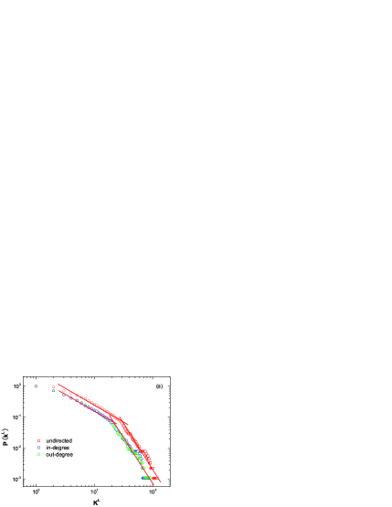
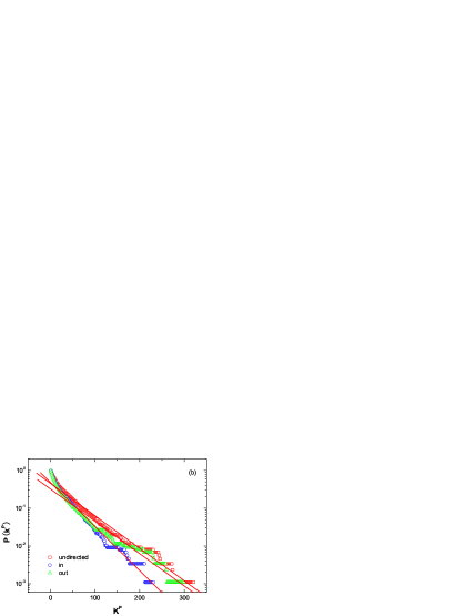
Figure 2: (a) Degree distributions in the space $L$ obey truncated power-law distributions with almost the same exponents. The turning points are at $k=20$ and $k=30$ respectively. (b) Degree distributions in the space $P$ all follow exponential distributions. (c) Positive correlation between in-degree and out-degree. (d) Unweighted degree under two spaces. Degree in the space $P$ is larger than in the space $L$.

III Topological properties

Table 2: Basic parameters for spaces $L$ and $P$. $n$ is the number of nodes and $m$ is the number of links. $\langle k\rangle$ is the average undirected degree. $\langle C\rangle$ is the average unweighted cluster coefficient. $\langle l\rangle$ is the average shortest path length.

Space	$n$	$m$	$\langle k_{un}\rangle$	$\langle C\rangle$	$\langle l\rangle$
Space $L$	878	7955	9.04	0.4002	3.60
Space $P$	878	24967	28.44	0.7061	2.66

III.1 degree distribution and degree correlations

First we examine the degree distributions in two spaces. Fig. 2 shows that in-degree, out-degree and undirected degree distributions in the space $L$ all follow truncated power-law distributions with nearly the same exponents. In-degree and out-degree obey the function $P(k)\sim k^{-1.7}$ before $k=20$. When $k>20$ their distribution curves bend down to the function $P(k)\sim k^{-2.95}$. Unweighted degree in the space $L$ has the same exponents of $-1.7$ and $-2.95$ but the critical point becomes $k=30$. Truncated power-law degree distributions are often observed in other transportation networks like the worldwide air transportation network GuimeraPNAS , China airport network Wli , U.S. airport network chiliping and the Italian airport network Guida . It is explained in Amaral that the connection cost prevents adding new links to large degree nodes. Analogous cost constraints also exist in the maritime transport network. Congestion in hub ports often makes ships wait outside for available berth for several days, which can cost ships extremely high expense. Consequently new links are not encouraged to connect to those busy ports.

While in the space $P$ three degree distributions all follow exponential distributions $P(k)\sim e^{\alpha k}$. The parameters are estimated to be $\alpha=0.0117$ for in-degree, and $\alpha=0.0085$ for out-degree, $\alpha=0.0086$ for unweighted degree. The property that degrees obey truncated power-law distributions in the space $L$ and exponential distributions in the space $P$ is identical to public transportation networks Sienkiewicz ; Xinping2 and railway networks Sen . Particularly the Indian railway network Sen has exponential degree distributions with the parameter $0.0085$ almost the same with in-degree and out-degree distribution in WMN.

Next, the relation between in-degree and out-degree is studied. Fig. 2(c) is a plot of out-degree $k_{out}$ vs. in-degree $k_{in}$. They have a positive correlation under two spaces. Out-degree climbs when in-degree increases. Evidently the in-out degree correlation is very strong.

Finally, we want to find out the relations between degrees under different spaces. Fig. 2(d) shows undirected degree in the space $P$ $k_{un}^{P}$ vs. undirected degree in the space $L$ $k_{un}^{L}$. All dots are above the diagonal, indicating the undirected degree in the space $P$ is larger than in the space $L$. It is understandable because of different definition of two spaces topology. In the space $P$ all stops in the same route are connected which surely increases degree of each node. Table 2 lists the basic properties of WMN in two spaces. Average undirected degree in the space $P$ is $28.44$, much larger than average undirected degree 9.04 in the space $L$.

III.2 Line length

Let’s denote line length, i. e. the number of stops in one line, as $l$. In Fig. 3 the probability distribution of line length $P(l)$ can be approximated as a straight line in the semi-log picture representing an exponential decay distribution $P(l)\sim e^{-\alpha l}$ with the parameter $\alpha=0.13$. It indicates there are much more short haul lines than long haul lines in maritime transportation. Long haul lines use large vessels and travel long distance from one region to another region while short haul lines as branch lines travel between several neighboring ports and provide cargos to main lines. For example, the line consisting of the following ports: Shanghai-Busan-Osaka-Nagoya-Tokyo-Shimizu-Los Angeles-Charleston-Norfolk-New York-Antwerp-Bremerhaven- Thamesport-Rotterdam-Le Havre-New York-Norfolk-Charleston-Colon-Los Angeles-Oakland-Tokyo-Osaka-Shanghai, is a typical long haul line connecting main ports in Asia and Europe, calling at ports for 24 times.

Figure 3: Probability distribution of line length. It can be approximated by a straight line in semi-log plot indicating an exponential decay.

III.3 Shortest path length

The frequency distributions of shortest path lengths $d$ in the spaces $L$ and $P$ are plotted in Fig. 4. The distribution in the space $L$ has a wider range than in the space $P$. The average shortest path length is 3.6 in the space $L$ and 2.66 in the space $P$ (see Table 2). This means generally in the whole world the cargo need to transfer for no more than 2 times to get to the destination. Compared with the network size $N=878$, the shortest path length is relatively small.

Figure 4: Frequency distributions of shortest path length under two spaces. The distribution in the space $L$ has a wider range than in the space $P$.

Figure 5: (a) Weight distributions in two spaces. (b) Undirected strength distributions in two spaces. (c) Relation between in-strength and out-strength in two spaces. (d) Correlations between strength and degree in two spaces. The slopes both equal to 1.3 approximately indicating nonlinear relationships in the spaces $L$ and $P$.

III.4 Weight and strength distribution

Usually traffic on the transportation network is not equally distributed. Some links have more traffic flow than others and therefore play a more important role in the functioning of the whole network. Weight should be addressed especially in transportation networks. Here we study four properties of weighted WMN: weight distribution, strength distribution, in-out strength relations and the relations between strength and degree. The results are displayed in Fig. 5.

First we examine weight distributions. In Fig. 5 (a) two weight distribution curves are approximately straight declining lines before $w=40$. The power-law distributions are estimated to be $P(w)\sim w^{-0.95}$ in the space $P$ and $P(w)\sim w^{-0.92}$ in the space $L$.

Next, Fig. 5 (b) shows the undirected strength distributions under two spaces both obey power-law behavior with the same parameter. The functions are estimated to be $P(s)\sim s^{-1.3}$.

And we also analyze the relation between in-strength and out-strength in two spaces. As we can see from Fig. 5 (c), in-out strength relation under the space $L$ is plotted as almost a straight line while the relation under the space $P$ has a slight departure from the linear behavior at large $s_{in}$ values. But clearly they are positively correlated.

Finally an important feature of weighted WMN, the relations between strength and degree, is investigated. Under two spaces the relations between undirected strength and undirected degree are both unlinear with the slope of the line approximately $1.3$, which means the strength increase quicker than the increase of degree. This is often occured in the transportation networks and has its implication in the reality. It’s easy for the port with many container lines to attract more lines to connect the port and thus to increase the traffic more quickly.

IV Hierarchy structure

In this section, we explore the network structure of WMN through studying both the weighed and unweighted versions of cluster coefficient and average nearest neighbors degree. Hierarchy structure and "rich club" phenomenon are unveiled. We conjecture this kind of structure is related to ship companies’ optimal behavior to minimize the transportation cost known as the hub-and-spoke model in transportation industry.

IV.1 Clustering

Figure 6: Cluster coefficients. $C(k)$ under two spaces both exhibit nontrivial behavior with decay curves as functions of degree $k$. And weighted versions of cluster coefficient are larger than unweighted cluster coefficient, indicating high traffic edges between interconnected vertices.

Cluster coefficient $c_{i}$ is used to measure local cohesiveness of the network in the neighborhood of the vertex. It indicates to what extent two individuals with a common friend are likely to know each other. And $C(k)$ is defined as cluster coefficient averaged over all vertices with degree $k$.

We plot $C(k)$ in Fig. 6. Either in the space $L$ or in the space $P$, $C(k)$ exhibits a highly nontrivial behavior with a decay curve as a function of degree $k$, signaling a hierarchy structure in which low degrees belong generally to well interconnected communities (high clustering coefficient), while hubs connect many vertices that are not directly connected (small clustering coefficient).

$C^{P}(k)$ lies above $C^{L}(k)$ and the average cluster coefficient of the network in the space $P$ is 0.7 larger than 0.4 in the space $L$. This can be explained by the fact that in the space $P$ each route gives rise to a fully connected subgraph. With high cluster coefficient 0.7 and small average shortest path length 2.66 in the space $P$, we conclude that the WMN, as expected, has the small-world property.

Weighed quantities for clustering and assortativity measures are first proposed in Barrat3 . Through the case study of WAN and SCN, Barrat3 demonstrates that the inclusion of weight and their correlations can provide deeper understanding of the hierarchical organization of complex networks. The weighted cluster coefficient is defined as:

$$c^{w}_{i}=\frac{1}{s_{i}(k_{i}-1)}\sum_{j,h}\frac{w_{ij}+w_{ih}}{2}a_{ij}a_{ih}a_{jh}$$ (7)

which takes into account the importance of the traffic or interaction intensity on the local triplets. And we define $C^{w}(k)$ as the weighted cluster coefficient averaged over all vertices with degree $k$. In real weighted network we may have two opposite cases of the relation between $C^{w}(k)$ and $C(k)$. If $C^{w}(k)>C(k)$ in the network, interconnected triplets are more likely formed by the edges with larger weights. If $C^{w}(k)<C(k)$ the largest interactions or traffic is occurring on edges not belonging to interconnected triplets.

In Fig. 6 we report weighted cluster coefficient under two spaces. Evidently the weighted cluster coefficient $C^{wP}(k)$ and $C^{wL}(k)$ are both above the corresponding unweighted cluster coefficient, i. e. $C^{wP}(k)\geq C^{P}(k)$, and $C^{wL}(k)\geq C^{L}(k)$. This indicates some closely interconnected nodes with large degrees have the edges with larger weights among themselves. In other words, high-degree ports have the tendency to form interconnected groups with high-traffic’s links, thus balancing the reduced clustering. This is so called "rich-club" phenomenon.

IV.2 Assortativity

Figure 7: Average degree of the nearest neighbors as functions of $k$. Inclusion of weight changes the behavior of $k_{nn}(k)$: assortative behavior in the small degree range but disassortative behavior in large degree range, to definite assortative behavior of $k^{w}_{nn}(k)$ in the whole $k$ spectrum.

There is another important quantity to probe the networks’ architecture: the average degree of nearest neighbors, $k_{nn}(k)$, for vertices of degree $k$. Average nearest neighbors degree of a node $i$ is defined as:

$$k_{nn,i}=\frac{1}{k_{i}}\sum_{j}a_{ij}k_{j}$$ (8)

Using $k_{nn,i}$, one can calculate the average degree of the nearest neighbors of nodes with degree $k$, denoted as $k_{nn}(k)$. The networks are called assortative if $k_{nn}(k)$ is an increasing function of $k$, whereas they are referred to as disassortative when $k_{nn}(k)$ is a decreasing function of $k$. As suggested in Barrat3 , weighted version of average degree of nearest neighbors is calculated by:

$$k^{w}_{nn,i}=\frac{1}{s_{i}}\sum_{j}a_{ij}w_{ij}k_{j}$$ (9)

From this definition we can infer that $k^{w}_{nn,i}>k_{nn,i}$ if the links with the larger weights are pointing to the neighbors with larger degrees and $k^{w}_{nn,i}<k_{nn,i}$ in the opposite case.

Both the weighted and unweighted average degree of nearest neighbors under two spaces are plotted in Fig. 7. The curve of $k^{P}_{nn}(k)$ lies above the curve of $k^{L}_{nn}(k)$. The $k^{L}_{nn}(k)$ and $k^{P}_{nn}(k)$ grow with the increase of degrees at small degrees but decline when degrees are large. The unweighted network exhibits assortative behavior in the small degree range but disassortative behavior in large range.

When we turn to the $k^{wL}_{nn}(k)$ and $k^{wP}_{nn}(k)$, the weighted analysis provides us a different picture. We can see that under two spaces the weighted average degree of nearest neighbors exhibits a pronounced assortative behavior in the whole $k$ spectrum. Since the number of WMN nodes is 878, this conforms with the empirical finding in Sienkiewicz that public transport networks are assortative when the number of nodes in the network $N>500$ and disassortative when $N<500$.

From the above discussion we can see that the inclusion of weight changes the behavior of cluster coefficient and average degree of nearest neighbors. This property is identical to the worldwide airport network Barrat3 and North America airport network Barrat4 . In both the airline transportation and maritime transportation networks, high traffic is associated to hubs and high-degree ports (airports) tend to form cliques with other large ports (airports). Their similar organization structure may have a similar underlying mechanisms. We conjecture that this is related to the hub-and-spoke structure which is widely adopted in practice by airline companies or ship companies to achieve the objective of minimizing the total transportation cost OKelly ; Robinson ; Moura ; Bryan .

Fig. 8 describes a typical hub-and-spoke structure which consists of three interconnected hubs and other nodes allocated to a single hub. In maritime transportation main liners travel between hubs handling large traffic while branch liners visit the hub’s neighboring ports to provide cargo for the main lines. This structure allows the carriers to consolidate the cargo in larger vessels to lower the transportation cost. This simple structure has the similar property of $C^{w}(k)>C(k),k^{w}_{nn}(k)>k_{nn}(k)$ with that of WMN. And it also displays rich-club phenomenon. We think it worths investigating the relations between ship companies’ optimal behavior and the real transportation network’s hierarchy structure and rich-club property.

Figure 8: A classical hub-and-spoke structure in maritime transportation. There are three central vertices having very strong links (high traffic) with each other and several nodes having weak links (low traffic) with hubs. It has the same property of $C^{w}(k)>C(k),k^{w}_{nn}(k)>k_{nn}(k)$ with that of WMN.

V Centrality measures

Figure 9: (a) Probability distribution of betweenness obeys truncated power-law distribution. (b) Betweenness is a straight line in log-log picture indicating a power-law relation with degree. The exponent in the space $L$ is estimated to be 1.66 and that in the space $P$ is estimated to be 1.93.

In this section we analyze two centrality measures in social network analysis Wasserman : degree and betweenness. The most intuitive topological measure of centrality is given by the degree: more connected nodes are more important. The distribution and correlations of degree has been discussed in Section IV.

Betweenness centrality is defined as the proportion of the shortest paths between every pair of vertices that pass through the given vertex $v$ towards all the shortest paths. It is based on the idea that a vertex is central if it lies between many other vertices, in the sense that it is traversed by many of the shortest paths connection couples of vertices. Hence we have

$$C_{i}^{B}=\frac{1}{(N-1)(N-2)}\sum_{j,k}\frac{n_{jk}(i)}{n_{jk}}$$ (10)

where $n_{jk}$ is the number of shortest paths between $j$ and $k$, and $n_{jk}(i)$ is the number of shortest paths between $j$ and $k$ that contain node $i$.

Correlations between two centrality measures are presented in Fig. 9(b). In both the spaces there is a clear tendency to a power-law relation with degree $k$: $C^{B}(k)\sim k^{\alpha}$ with $\alpha=1.66$ in the space $L$ and $\alpha=1.93$ in the space $P$. The power-law correlations between degree and betweenness is also found in bus transportaiton networks Sienkiewicz ; Ferber and ship transport network Xinping1 . It’s worth noting that this power-law relations together with the truncated scale-free behavior of the degree distribution implies that betweenness distribution should follow a truncated power law. This behavior is clearly identified in Fig. 9(a). We find the betweenness centrality has two-regime power-law behavior $P(C^{B})\sim C^{-\alpha}$. For the two spaces, exponents are almost the same: $\alpha=0.14$ at small degree regime and $\alpha=1.0$ at large degree regime.

The power-law relations between degree and betweenness suggest that they are consistent with each other. It is proved in the comparison of each port’s degree and betweenness. The 25 most connected ports are listed in Table. 3. Singapore is the most busy ports in the world with the largest degree and betweenness. Antwerp and Bushan are the second and third either in degree or in betweenness measures. Only 5 ports in these ports are not listed in the 25 most central ports in betweenness measure. WMN is not like the case of the worldwide airline network GuimeraPNAS which has anomalous centrality due to its multicommunity structure. The difference may due to the fact that there are less geographical and political constraints in maritime transportation than in air transportation. Ships can travel longer distance than airplanes. And airports are usually classified into international and domestic airports and international airlines are limited to connect international airports instead of domestic airports. So there are distinct geographically constrained communities in WAN. In the maritime transportation there are no such constraints. Sea ports basically are all international ports with the possibility to connect to any other sea ports in the world.

Table 3: The 25 most connected ports in the worldwide maritime transportation network. * These ports are not among the 25 most central ports.

Rank	Ports	Degree	Betweenness	Region
1	Singpore	120	124110.1258	Asia
2	Antwerp	102	113368.6161	Europe
3	Bushan	92	69094.7490	Asia
4	Rotterdam	87	78097.8754	Europe
5	Port Klang	83	62111.6226	Asia
6	Hongkong	78	46072.9799	Asia
7	Shanghai	75	37748.4316	Asia
8	Hamburg	60	40362.4625	Europe
9	Valencia	60	27346.0956	Europe
10	Le Havre	58	48231.1636	Europe
11	Gioia Tauro	55	20148.4667	Europe
12	Yokohama	54	19716.7287	Asia
13	Kaohsiung	52	15363.5781	Asia
14	Port Said*	52	16121.8476	Africa
15	Bremerhaven	50	24998.9088	Europe
16	Colombo*	48	15128.362	Asia
17	Tanjung Pelepas	46	18735.1267	Asia
18	Jeddah*	45	8570.7724	Middle East
19	Jebel Ali	44	20137.5255	Middle East
20	Ningbo*	44	12315.9515	Asia
21	Algeciras	43	18701.2619	Europe
22	Barcelona*	43	15256.3903	Europe
23	Kobe	43	8869.7313	Asia
24	New York	42	25935.6692	North America
25	Kingston	41	23281.3223	Latin America

Figure 10: The geographical distribution of 25 most connected ports. They are located along east-west lines, including 13 ports in Asia and Middle East, 9 in Europe, 1 in Africa, 1 in North America and 1 in Latin America.

In Fig. 10 we plot the 25 most connected ports on the world map. They show unbalanced geographical distribution mainly located in Asia and Europe, including 13 ports in Asia and Middle East, 1 in Africa, 9 in Europe, 1 in North America and 1 in Latin America. Particularly they are located along the east-west lines. Lines in maritime transportation are usually divided into east-west lines, north-south lines and south-south lines Rodrigue ; Fremont . The fact that 25 most connected ports in the world are in east-west trade routes represents rapid growth and large trade volume in Europe-America, Asia-America and Asia-Europe trade maritimereport .

VI Conclusion

In this paper we have presented an empirical study of the worldwide maritime transportation network (WMN) under different representations of network topology. We study the statistical properties of WMN and find that WMN is a small world network with power law behavior. There are strong correlations in degree-degree, strength-degree and betweenness-degree relations. Central nodes are identified based on different centrality measures. Based on the analysis of weighted cluster coefficient and weighted average nearest neighbors degree, we find that WMN has the same hierarchy structure and "rich-club" phenomenon with WAN. We conjecture that this structure is related to optimal behavior both existing in air transportation and maritime transportation. So our future research direction is the evolution modeling of WMN using optimal behavior to reproduce real properties in WMN.

References

- (1) A. -L. Barabasi, R. Albert, Nature 286 (1999) 509.
- (2) M. E. J. Newman, Proc. Natl. Acad. Sci. USA 98 (2001) 404.
- (3) H. Jeong B. Tombor R. Albert Z. N. Oltvai, A.-L. Barabasi, Nature 407 (2000) 651.
- (4) L. A. N. Amaral, A. Scala, M. Barthelemy, H. E. Stanley, Proc. Natl. Acad. Sci. USA 97 (2000) 11149.
- (5) R. Guimera, S. Mossa, A. Turtschi and L. A. N. Amaral, Proc. Natl. Acad. Sci. USA 102 (2005) 7794.
- (6) W. Li, X. Cai, Phys. Rev. E 69 (2004) 046106.
- (7) L.P. Chi, R. Wang, H. Su, X.P. Xu, J.S. Zhao, W. Li, X. Cai, Chin. Phys. Lett. 20 (8) (2003) 1393.
- (8) M. Guida, F. Maria, Chaos soitions and fractals 31 (2007) 527.
- (9) Xinping Xu, Junhui Hu, Feng Liu, Chaos 17, 023129 (2007).
- (10) Julian Sienkiewicz, Janusz Holyst, Phys. Rev. E 72 (2005) 046127 .
- (11) Xinping Xu, Junhui Hu, Feng Liu, Lianshou Liu, Physica A 374 (2007) 441.
- (12) Liping et al, Chin. Phys. Lett. 23 (12) (2006) 3384.
- (13) C. von Ferber, T. Holovatch, Yu. Holovatch, and V. Palchykov, Arxiv 0803.3514v1, 2008.
- (14) V. Latora, M. Marchiori, Physica A 314 (2002) 109.
- (15) P. Sen, S. Dasgupta, A. Chatterjee, P.A. Sreeram, G. Mukherjee, S.S. Manna, Phys. Rev. E 67 (2003) 036106.
- (16) W. Li, X. Cai, Physica A 382 (2007) 693.
- (17) United Nation conference on trade and development, Review of maritime transport 2007, http://www.unctad.org/en/docs/rmt2007en.pdf
- (18) Jean-Paul Rodrigue, Claude Comtois, The geography of transport systems, New York: Routledge, 2006.
- (19) http://www.ci-online.co.uk/
- (20) A. Barrat, et al., Proc. Natl. Acad. Sci. USA 101 (11) (2004) 3747.
- (21) A. Barrat, M. Barthélémy, A. Vespignani, J. of Stat. Mech. (2005) P05003.
- (22) M. O’Kelly, Journal of transport geography, 6 (3) (1998) 171.
- (23) Ross Robinson, Maritime Policy and Management 25 (1) (1998) 21.
- (24) M. C. Moura, M. V. Pato, A. C. Paixa, Maritime Policy and Management 29 (2) (2002) 135.
- (25) Bryan and M. O’Kelly, Journal of regional science, 39 (2) (1999) 275.
- (26) S. Wasserman, K. Faust, Social networks analysis, Cambridge University Press, Cambridege, 1994.
- (27) A. Fremont, Journal of transportation geography, 15 (2007) 431.