Towards isotropic negative magnetics in the visible range

Abstract

The idea of isotropic resonant magnetism in the visible range of frequencies known from precedent publications is developed having in mind achievements of the modern chemistry. Plasmonic colloidal nanoparticles covering a silica core form a cluster with resonant and isotropic magnetic response. Two approximate models giving the qualitative mutual agreement are used to evaluate the magnetic polarizability of the cluster. It is shown that the electrostatic interaction of nanocolloids decreases the resonant frequency of an individual complex magnetic scatterer (nanocluster) compared to the previously studied variant of a planar circular nanocluster with same size. This means the reduction of the optical size of nanoclusters that presumably allows one to avoid strong spatial dispersion within the frequency range of the negative permeability.

I Introduction

The interest in artificial resonant magnetism in the optical range which was recently inspired by the development of metamaterial science (see e.g. in Engheta1 ; Caloz ) is expected to grow after successful demonstration of the subwavelength optical imaging obtained in the far zone of objects with the use of so-called hyperlenses Zhang ; Smol . Hyperlenses transform evanescent waves into propagating ones and create the spatially magnified optical images keeping subwavelength details of the objects.

Known hyperlenses operate with TM-polarized waves. This polarization is related to the negative permittivity of metals (which are used by known hyperlenses) in the visible frequency range. Similar operation with the TE-polarized light would require materials with negative permeability.

Materials with negative $\mu$ in the visible range do not exist in nature. Recently, many attempts to engineer such materials were reported. They include, for example, lattices of paired plasmonic nanowires, nanoplates, nanocones, fishnets, and plasmonic split rings 4 ; 5 ; 6 ; 8 ; 9 ; fishnet ; fishnet1 ; 11 . These structures are all geometrically strongly anisotropic. The strongest magnetic response corresponds to one specific direction of the propagation of electromagnetic wave. Notice, that in cited papers the magnetic response of these structures was reported only for this single direction. The possibility to use strongly anisotropic artificial magnetic media in superlenses and hyperlenses has not yet been studied.

The first work devoted to the possibility of the isotropic optical magnetism that cannot be achieved in the mentioned anisotropic structures was, to our knowledge, Engheta . The idea of the present paper is to link this resonant magnetism to the existing technology and to find the design which ensures the real isotropy of the resonant permeability, i.e. absence of strong spatial dispersion. We use the term strong spatial dispersion for the case when the dispersion diagram of the lattice is quantitatively different from the dispersion in any continuous media. Weak spatial dispersion is a special term applied to designate effects of artificial magnetism and bianisotropy in composite media biaha .

In Engheta one suggested to prepare optical magnetic media using plasmonic (colloids of noble metals) nanospheres arranged in nanorings. In high-frequency magnetic field ${\bf H}_{0}$ nanocolloids are polarized in the azimuthal direction with respect to this field. To obtain an isotropic resonant magnetic medium one should fabricate a dense array of nanorings lying in 3 mutually orthogonal planes. The dense isotropic package means that the array of nanorings must be a fcc or a bcc lattice, that allows us to consider the structure as a photonic crystal. The theoretical prediction of Engheta shows that in this case the resonance of the effective permeability $\mu_{\rm eff}$ can be strong enough so that the real part of $\mu_{\rm eff}$ takes negative values. However, from Engheta it has not yet been clear how to fabricate these structures and their isotropy was not proved. In fact, an isotropic artificial magnetism is not possible for photonic crystals (lattices with strong spatial dispersion).

Formally, the resonant magnetic permeability as well as the permittivity can be attributed to photonic crystals as well (see e.g. bred4 ; 13 ; 14 ). However, at frequencies where a cubic lattice becomes a photonic crystal the refraction index and the wave impedance both become strongly dependent on the propagation direction agranovich . This implies that effective material parameters $\varepsilon_{\rm eff}$ or/and $\mu_{\rm eff}$ of the crystal are very different for a wave propagating along one of the lattice axes and for a wave tilted with respect to this axis. This evidently means the absence of the isotropy. Of course, the random mixture of particles is more optically isotropic than the lattice with the same concentration of particles. However, in the present case the requirement of the negative magnetic response of the composite medium obviously implies the very dense packaging of magnetic scatterers. In the present case we cannot suppress the spatial dispersion using the randomization of the array.

The comparison of the approximate dispersion diagram for the homogenized lattice with the exact dispersion diagram was done in some papers, e.g. in Li ; Belov. In Li the fcc (face-centered cubic) and bcc (body-centered cubic) lattices of metal-covered dielectric spheres were studied. It was found that in fcc and bcc lattices the spatial dispersion effects arise within the frequency band of the plasmonic resonance. The spatial dispersion in this region leads to closing the resonance band-gap with simultaneous strong anisotropy of the lattice refraction index. These effects correspond to the frequencies at which the distance between adjacent particles centers exceeds one quarter of the wavelength in the matrix.

Unfortunately, in the known literature there are no general results for the frequency intervals where the effects of strong spatial dispersion arise in lattices. Of course, it is clear that the frequency range corresponding to $D/\lambda\geq 0.5$ definitely implies the strong spatial dispersion since $\lambda=2D$ is the Bragg resonance condition. In lattices of strongly scattering inclusions the condition of the absence of strong spatial dispersion becomes more restrictive since the polarization of inclusions shortens the effective wavelength $\lambda_{\rm eff}$ compared to $\lambda$.

It is known that the artificial resonant magnetism in arrays of small complex-shape metal particles at microwaves practically corresponds to relation $D_{p}/\lambda_{r}>0.1$, where $D_{p}$ is the typical size of the particle biaha ; biama and $\lambda_{r}$ is the wavelength of the magnetic resonance of a particle in host medium. Notice, that the ratio $D_{p}/\lambda\approx 0.1\dots 0.15$ is practically achievable, e.g. for well-known double split-ring resonators (SRRs). SRRs of this optical size can be considered as small enough to avoid the strong spatial dispersion in a compact lattice. Then we can consider the low-frequency stop-band of this lattice associated with the resonance of SRRs as the effect of the negative permeability. Really, magneto-electric media are opaque when their material parameters have different signs.

However, the metamaterial suggested in Engheta corresponds to a quite large optical size of a magnetic scatterer at its resonance, where the condition $D_{p}/\lambda_{r}<0.15$ is far from being fulfilled. Really, consider the results for $\mu_{\rm eff}$ illustrated by Fig. 2 (a,b) of Engheta . The negative permeability was theoretically achieved at $630$ or $680$ THz with nanorings of the following geometry. Six or four metal nanospheres of radius $a_{p}=16$ nm are centered at the circle of radius $R_{0}=40$ or $R_{0}=38$ nm. This means that the size $D_{p}$ of the effective magnetic particle (i.e. the distance between the edges of opposite metal nanospheres) is $112$ or $108$ nm. The wavelength in the host medium with background permittivity $\varepsilon_{h}=2.2$ at $630$ THz is equal to $\lambda_{r}=323$ nm. Then the size of the nanoring from 6 spheres is $D_{p}\approx 0.35\lambda_{r}$ i.e. the optical size is rather large. The packaging of these nanorings in the host medium was assumed in Engheta to be very dense, namely corresponding to their concentration $N_{NR}=(108)^{-3}$ nm^-3. This concentration is physically achievable for a bcc or a fcc lattice of nanorings. However, even so dense packaging corresponds to the distance between the centers of adjacent nanorings $D\approx 0.4\lambda_{r}$. Having in mind results of Li we believe that in this case the strong spatial dispersion arises and the isotropic magnetism is impossible.

The clear way to decrease spatial dispersion in a lattice of magnetic scatterers i.e. to suppress the angular dependence of $\mu_{\rm eff}$ is to decrease the size of a scatterer keeping its magnetic polarizability. In this way we will also decrease the optical distance between the centers of adjacent magnetic particles. Below we modify the design of magnetic particles suggested in Engheta in this way. We obtain the ratio $D_{p}/\lambda_{r}\approx 0.2\dots 0.25$ which is presumably below the range of the strong spatial dispersion. Simultaneously, we link our design to existing nanotechnologies.

II Core-shell magnetic clusters

The design of the optical magnetic scatterer suggested in this paper is based on the possibility to fabricate arrays of silver or gold colloidal nanoclusters located on spherical dielectric cores in a liquid host medium. The fabrication technology uses self-assembled adhesion of metal nanospheres on the silica core. The idea of such self-assembling aggregates was probably first realized in Morn . However, this process led to the complete covering of the silica core by contacting gold nanoparticles. The process chemically stimulated by some acids which allowed one to control its speed and to obtain the needed number of nanocolloids per one core was described in Mornet . Later, nanoclusters comprising few tens of colloidal particles on a silica core of diameter of the order 100 nm were reported in works Jiang . For obtaining the maximal electromagnetic response for given sizes (of the core and of the nanocolloids) their number $N_{\rm tot}$ per one nanocluster should be as large as possible. However, it is difficult in this way to prevent the touching of nanocolloids which is destructive for their plasmonic resonance that will degrade due to the tunneling of electrons between nanocolloids. Practically, minimal separation $d$ between nanocolloids should be comparable with the radius of colloidal particles $a_{p}$. Below we respect the condition $d\approx a_{p}/2$ that restricts $N_{\rm tot}$. This can be practically obtained using the technology described in new1 and new2 . In these works the silica core of diameter 100 nm (the technology allows in principle to reduce this size to 20-30 nm) was covered by mutually touching polystyrene nanospheres. Instead of simple polystyrene nanospheres one can use core-shell particles with plasmonic nanocolloids as cores. This method will allow us to reliably control the separation $d$ between colloidal particles which is simply equal to the double thickness of the polystyrene shell.

Such a nanocluster is shown in Fig. 1 (a) (a general view) and (b) (a cross section). It should have the isotropic resonant response to the electromagnetic field of light. At one frequency the induced electric dipole dominates, and the polarization of colloidal particles is parallel to the electric field of light. At another frequency the induced magnetic dipole dominates, and the polarization of colloidal particles is azimuthal with respect to the magnetic field. In other words, the applied magnetic field form the effective nanorings of colloidal spheres glued to the silica core. Both electric and magnetic resonant frequencies origin from the plasmonic resonance of an individual colloidal nanosphere. In this paper we study only the magnetic resonance of such a nanocluster. Therefore we call it a magnetic nanocluster (MNC). Bulk arrays of MNC can be created not only in liquid but also in porous matrices where the separation between the pores should be small enough to obtain the high concentration of MNC and a strong magnetic response of the medium.

Below we will see that the frequency of the magnetic resonance of MNC is strongly reduced compared to the frequency $\Omega_{p}$ of the plasmonic resonance of a single nanocolloid. This effect results from the strong electrostatic coupling between the nanocolloids in the MNC. This electrostatic coupling exists also in a single nanoring studied in Engheta , and it leads to a certain reduction of the magnetic resonance frequency compared to $\Omega_{p}$. However, in the present geometry this reduction is much stronger since the most important electrostatic interaction is that between colloids having parallel electro-dipole moments.

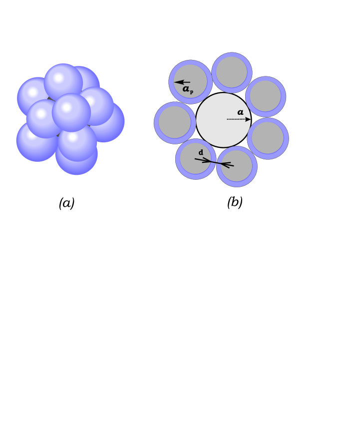
Figure 1: A magnetic nanocluster (a bulk isotropic scatterer with the magnetic resonance): (a) – a general view of a cluster of metal nanocolloids with dielectric core, (b) – the resonant azimuthal electric polarization $\vec{P}_{\phi}$ is excited in the discrete ”shell” formed by plasmonic nanocolloids when the applied field is the optical magnetic field directed along $z$.

The total number $N_{\rm tot}$ of colloidal nanospheres per one MNC can be controlled by the self-assembling technological process. Also, it can be adjusted by properly chosen initial concentrations of nanocolloids and silica spheres in the host liquid. $N_{\rm tot}$ can be expressed through the core radius $a$, the colloid radius $a_{p}$ and the separation $d$ between metal spheres (see Fig. 1):

$$N_{\rm tot}=\left[{4\pi(a+a_{p}+d/2)^{2}\over(2a_{p}+d)^{2}}\right].$$ (1)

Here $[A]$ denotes the integer part of the number $A$. In this formula the curvature of the portion $\Delta$ of the spherical surface with radius $R_{0}=a+a_{p}+d/2$ which is cut of the sphere of radius $R_{0}$ (this sphere centers the nanocolloids and their dipole moments are located on it) by one core-shell particle of radius $a_{p}+d/2$ is neglected. In other words, in our calculations the surface $\Delta$ of the effective sphere $R_{0}$ per one colloidal particle is assumed to be a planar square with side $2a_{p}+d$.

III Two models of MNC

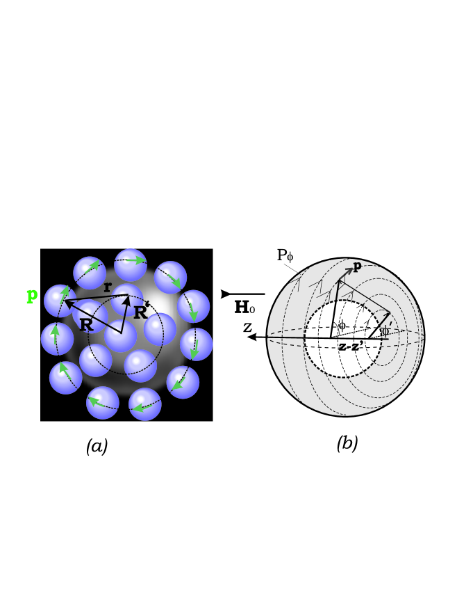
Figure 2: Two models of the magnetic polarization of MNC in the applied magnetic field directed along $z$: (a) – nanocolloids form regular rings around the $z-$axis, the colloidal particles are equidistant in the rings of radiuses $R_{j}$ (induced dipole moments are shown by bold arrows) and the rings are equidistant; (b) – nanocolloids form around the core (shown as a dashed circle) an effective continuous shell with azimuthal bulk polarization $P_{\phi}$. The shell of thickness $2a_{p}+d$ can be characterized by resonant isotropic permittivity $\varepsilon_{L}$.

Two approximate models for obtaining the magnetic polarizability $a_{mm}$ of a MNC are illustrated by Fig. 2 (a) and (b). The agreement of their results can be hopefully considered as a validation of these results. These models describe in two different ways the electromagnetic interaction of colloidal particles. In the first model the nanocolloids on the dielectric core are assumed to form regular rings around the $z-$axis. The rings of radiuses $R_{j}$ are distanced by $a_{p}/2$ from one another. The distance between the nanoparticles in any ring is also equal to $d=a_{p}/2$. The presence of the polystyrene shell of nanocolloids does not influence to the result, since the permittivity of the shell is equal to that of the matrix ($\varepsilon_{h}=2.2$).

In the second model the discrete structure of core-shell plasmonic nanoparticles on the central silica core is treated as a nanolayer of effective medium of thickness $\delta=2a_{p}+d$ covering the silica core. The azimuthal electro-dipole polarization $P_{\phi}$ and the isotropic permittivity $\varepsilon_{L}$ of this layer can be easily calculated and we find $a_{mm}$ in the closed form calculating the magnetic moment of this homogenized shell.

The presence of the central silica core also does not influence to the result due to the absence of its electric polarization by the applied magnetic field and smallness of its magnetic moment which is not resonant. It was checked analytically that the interaction of this small magnetic moment with electro-dipole moments of colloidal particles is negligible. The permittivity of the silica core $\varepsilon_{s}=4>\varepsilon_{h}=2.2$ influences only weakly to the response of colloidal spheres. The polarizability $\alpha$ of a single colloidal particle is assumed to be the same as if nanocolloids were located in the uniform medium with permittivity $\varepsilon_{h}$:

$$\alpha=\left[\left(4\pi a_{p}^{3}\varepsilon_{0}\varepsilon_{h}{\varepsilon_{m}-\varepsilon_{h}\over\varepsilon_{m}+2\varepsilon_{h}}\right)^{-1}-i{k^{3}\over 6\pi\varepsilon_{0}\varepsilon_{h}}\right]^{-1}.$$ (2)

Here $\varepsilon_{m}$ is the permittivity of the metal which is taken in the same form as in Engheta :

$$\varepsilon_{m}=\varepsilon_{i}-{(2\pi f_{p})^{2}\over\omega^{2}}+i{(2\pi)^{2}f_{p}f_{d}\over\omega^{2}}.$$ (3)

For silver colloids we have the plasma linear frequency $f_{p}=2175$ THz, the damping frequency $f_{d}=4.35$ THz and the ultraviolet permittivity $\varepsilon_{i}=5$ Engheta .

As it was explained in Engheta the magnetic moment of nanorings is excited by the magnetic field of the light wave. To calculate the magnetic polarizability of a MNC we assume that it is excited by magnetic field polarized along $z$ [see Fig. 1 (b)] that in the model of the magnetic excitation assume to be uniform across the circle of radius $R_{0}$ and varying with time as $\exp(-i\omega t))$ with amplitude $H_{0}$. From Maxwell’s equations this applied magnetic field $\vec{H}_{a}$ is associated with the azimuthal electric field $\vec{E}_{a}$ vanishing at the center of MNC:

$$\vec{H}_{a}=\vec{z}_{0}H_{0},\quad\vec{E}_{a}=\vec{\phi}_{0}(i\eta H_{0}kR),$$ (4)

where $\eta=\sqrt{\mu_{0}/\varepsilon_{0}\varepsilon_{h}}$ is the wave impedance of the host medium of permittivity $\varepsilon_{h}$. Unit vectors $\vec{z}_{0}$ and $\vec{\phi}_{0}$ correspond to the cylindrical coordinates $(R,\phi,z)$ shown in Fig. 1 (b). In fact, the applied electric field given by (4) is associated with slightly non-uniform magnetic field $\vec{H}_{a}=\vec{z}_{0}H_{0}(1-k^{2}R^{2}/2)$, but this small correction to the applied magnetic field matters nothing for our model. We calculate the magnetic moment of MNC induced by $\vec{H}_{a}$ whose amplitude at the center of MNC is $H_{0}$ through the electric polarization of nanocolloids by the electric field associated with $\vec{H}_{a}$.

The $\phi$-oriented dipole moments $p_{j}$ of colloidal particles of any $j$-th ring are identical in polar coordinates. The $z$-directed magnetic moment $m_{j}$ of the j-th ring can be found using formula (8) of Engheta . The total magnetic polarizability of MNC is then obtained as $a_{mm}=\sum a_{mm}^{(j)}$, where $a_{mm}^{(j)}=m_{j}/H_{0}$.

Notice, that the obvious (not sufficient) condition of the absence of spatial dispersion in a bulk array of MNC is the independence of the magnetic polarizability $a_{mm}$ of an individual MNC on the distribution of the applied magnetic field around the center of MNC, if the condition of the magnetic excitation is respected: $\vec{H}_{a}(R=0)=\vec{z}_{0}H_{0},\ \vec{E}_{a}(R=0)=0$. This condition can be satisfied for example by a standing plane wave, i.e. a pair of plane waves travelling along the $x-$axis:

$$\vec{H}_{a}=\vec{z}_{0}{H_{0}\over 2}(e^{-jkx}+e^{jkx}),\quad\vec{E}_{a}=\vec{y}_{0}{\eta H_{0}\over 2}(e^{-jkx}-e^{jkx}).$$

The comparison of $a_{mm}$ calculated for this azimuth-dependent excitation of MNC and that calculated for excitation (4) would be a useful exercise, and we plan it for the next paper. It could indicate the frequency bounds of the spatial dispersion related to the finite size of MNC. However, in the present paper we restrict the analysis by a more simple excitation case (4).

In both models the reduction of the resonance frequency of MNC compared to the plasmonic resonance $\Omega_{p}$ of the individual colloidal particle in the host medium with $\varepsilon_{h}=2.2$ is determined by the electromagnetic coupling of colloids. In fact, this reduction will be even stronger than it is predicted below. This is because the presence of the silica core makes the effective host medium permittivity slightly larger than $\varepsilon_{h}$. We neglect this small effect for simplicity of the model, however, its role is positive.

III.1 The model of regular rings

Consider a dipole $\vec{p}=p(j)\vec{\phi}_{0}$ shown in Fig. 1 (b) that belongs to the j-th effective ring of MNC. Assume that $N_{\rm tot}\gg 1$ (practically the model is applicable when $N_{\rm tot}>15\dots 20$). Then it is easy to show using auxiliary spherical coordinates and formula (1) for $N_{\rm tot}$ that the radius of the j-th ring is approximately equal to $R_{j}\approx R_{0}\sin({2j\sqrt{\pi/N_{\rm tot}}})$. The $z-$coordinate of the j-th ring is $z(j)\approx R_{0}\cos({2j\sqrt{\pi/N_{\rm tot}}})$. The number of dipoles $N_{j}$ in the ring is equal $N_{j}\approx 2\pi R_{j}/(2a_{p}+d)$. The number of such rings in MNC is equal $N_{r}\approx\sqrt{\pi N_{\rm tot}}/2$. The cylindrical coordinates of the dipole $\vec{p}$ in the j-th ring are $z=z_{j}$, $R=R_{j}$, $\phi=2\pi q/N_{j}$ where $q=0\dots(N_{j}-1)$ is the integer number determining the position of the dipole within the ring.

The field produced by the dipole $\vec{p}$ at the point with coordinates $(z^{\prime},R^{\prime},\phi^{\prime})$ can be found from the standard formula:

$$\vec{E}(\vec{R},\vec{R}^{\prime})={1\over 4\pi\varepsilon_{0}\varepsilon_{h}}\left[k^{2}(\vec{r}\times\vec{p})\times\vec{r}{e^{-jkr}\over r^{3}}+(3\vec{r}\vec{p}\cdot\vec{r}-\vec{p}r^{2})\left({e^{ikr}\over r^{5}}-{ike^{ikr}\over r^{4}}\right)\right].$$ (5)

Here $r=\sqrt{R^{2}+R^{{}^{\prime}2}-2RR^{\prime}\cos(\phi-\phi^{\prime})+(z-z^{\prime})^{2}}$ is the distance between radiating $p(j)$ and receiving $p(n)$ dipoles of MNC. Due to the azimuthal symmetry of the problem only the $\phi-$th component of the field produced by all rings of dipoles $p(j)$ is nonzero at the center of the receiving dipole $p(n)$, i.e. at point $(z^{\prime},R^{\prime},\phi^{\prime})$. In other words the local electric field acting on the dipole $p(n)$ is orthogonal to the vector $\vec{R}^{\prime}$ shown in Fig. 1 (b). Respectively, only the azimuthal component of the vector $\vec{E}(\vec{R},\vec{R}^{\prime})$, should be taken into account.

From (5) the scalar interaction coefficient of dipoles $p(j)$ and $p(n)$ can be easily derived. It is defined as the $\phi$-th component of the field produced by the unit azimuth-oriented dipole located at point $(z=z_{j},R=R_{j},\phi=2\pi q/N_{j})$ and calculated at point $(z^{\prime}=z_{n},R^{\prime}=R_{n},\phi^{\prime}=2\pi s/N_{n})$:

$$Q_{qs}^{nj}={e^{ikr}\over 4\pi\varepsilon_{0}\varepsilon_{h}r^{5}}\left[(kr)^{2}(R^{{}^{\prime}2}+(z-z^{\prime})R^{\prime}-RR^{\prime}+\cos(\phi-\phi^{\prime})(R^{2}+(z-z^{\prime})R)-RR^{\prime})\right.$$

$$\left.-3RR^{\prime}\sin^{2}(\phi-\phi^{\prime})(1-ikr)-\cos(\phi-\phi^{\prime})(1-ikr)r^{2}\right].$$ (6)

The dipole moment of the receiving dipole is equal to $p=\alpha E^{\rm loc}$. Here the local field is the sum of the external electric field (4) $E_{a}(R^{\prime})=(iH_{0}\eta kR^{\prime}/2)$ and all dipole fields:

$$E^{\rm loc}=E_{a}(R^{\prime})+p(j)\sum\limits_{s,j}Q_{qs}^{nj}.$$

This way we obtain the system of equations for dipole moments of colloidal nanospheres of any ring:

$${1\over\alpha}p(n)={iH_{0}\omega\mu_{0}R(n)\over 2}+p(n)\sum\limits_{q=1}^{N_{n}-1}Q_{0q}^{nn}+\sum\limits_{j\neq n}^{N_{r}}p(j)\sum\limits_{q=0}^{N_{j}-1}Q_{0q}^{nj}.$$ (7)

Here the term with $Q_{0q}^{nn}$ describing the interaction of the dipole $p(n)$ located at ($z^{\prime}=z_{n},R^{\prime}=R_{n},\phi^{\prime}=0$) with other dipoles of the same n-th ring is shared out. The expressions for coefficients $Q_{0q}^{nn}$ entering this term and given by (6) with $z=z^{\prime}$ are described by (6). There is no coefficient $Q_{00}^{nn}$ in (7) since the summation starts from $q=1$ (see also in Engheta ).

Solving the system (7) we find all dipole moments $p(n)$. The magnetic moment of $j$-th ring is calculated as in Engheta :

$$m_{j}={-i\omega p(j)N_{j}R_{j}\over 2}.$$ (8)

Then we obtain the magnetic polarizability of the MNC as the sum of $m_{j}$ letting $H_{0}=1$:

$$a_{mm}={{-i\omega\over 2}}\sum\limits_{j=1}^{N_{r}}p(j)N_{j}R_{j}.$$

The relative effective permeability of the composite medium is given by Engheta :

$$\mu_{\rm eff}=1+{1\over N_{MNC}^{-1}a_{mm}^{-1}-{1\over 3}}.$$ (9)

Here $N_{MNC}$ is the volume concentration of MNC that can be expressed though the effective volume per one magnetic scatterer $N_{MNC}=1/V_{0}=1/D^{3}$. In simple cubic lattices $D\geq D_{p}=2(a+2a_{p})$, and $D$ is the unit cell size. However a more compact arrangement of MNC is also possible when $D<D_{p}$ and $N_{MNC}>1/D_{p}^{3}$.

The inverse polarizability of a nanocolloid in (7) corresponds to formula (2) and contains the term $(-i{k^{3}/6\pi\varepsilon_{0}\varepsilon_{h}})$ that describes the radiation damping. The radiation damping of the magnetic dipole with magnetic polarizability $a_{mm}$ should be described by the term $(-i{k^{3}/6\pi})$ Engheta . It is known that the radiation damping is cancelled out in regular 3D arrays and for regular lattices we should have used instead of (9) the relation Engheta :

$$\mu_{\rm eff}=1+{1\over N_{MNC}^{-1}\left(a_{mm}^{-1}+i{k^{3}\over 6\pi}\right)-{1\over 3}}.$$ (10)

However, the dissipative losses due to the plasmonic resonances of metal nanospheres strongly dominate over the contribution of radiation losses into the imaginary part of the permeability, i.e. the difference in results of (9) and of (10) is negligible.

III.2 The model of an effective shell

Replacing the discrete plasmonic structure by the continuous shell we introduce the bulk polarization $P_{\phi}$ that can be expressed through the averaged $\phi-$polarized electric field $E_{\rm av}$ in this shell and its unknown permittivity $\varepsilon_{L}$:

$$P_{\phi}=\varepsilon_{0}(\varepsilon_{L}-\varepsilon_{h})E_{\rm av}$$ (11)

The field $E_{\rm av}$ is related with the local field acting on any colloidal nanosphere by the Clausius-Mossotti relation:

$$E_{\rm av}=E_{\rm loc}-{p\over 3V_{1}\varepsilon_{0}\varepsilon_{h}}.$$ (12)

Here $V_{1}=2a_{p}(2a_{p}+d)^{2}$ is the volume per one colloidal nanosphere and $p=P_{\phi}V_{1}$ is the dipole moment of the reference nanosphere. Using the formula $p=\alpha E_{\rm loc}$ together with (11) and (12) we come to the Lorentz-Lorenz formula:

$$\varepsilon_{L}=\varepsilon_{h}\left(1+{3\over{3\varepsilon_{0}\varepsilon_{h}V_{1}\over\alpha}-1}\right).$$ (13)

The definition of the magnetic moment of any volume $V$ comprising polarization currents $\vec{j}$ reads as:

$$m={1\over 2}\int\limits_{V}\vec{j}\times\vec{r}dV.$$

It can be rewritten for the MNC in terms of the bulk polarization $P_{\phi}$:

$$m={-i\omega\over 2}\int\limits_{V_{L}}P_{\phi}R\,dV.$$ (14)

Here $V_{L}=4\pi R_{0}^{2}(2a_{p})=8\pi a_{p}(a+a_{p})^{2}$ is the volume of the spherical layer with central radius $R_{0}$ and the thickness $2a_{p}$. The integration of the bulk polarization across this layer can be replaced by simple product $P_{\phi}(2a_{p})$. The polar radius $R$ that enters (14) can be expressed in spherical coordinates as $R(\theta)=R_{0}\sin\theta$. After substitution of (11) into (14) we obtain:

$$m={-i\omega\varepsilon_{0}a_{p}(\varepsilon_{L}-\varepsilon_{h})R_{0}^{2}}\int\limits_{0}^{2\pi}\,d\phi\int\limits_{0}^{\pi}\,d\theta\sin\theta E_{\rm av}(\theta)R(\theta).$$ (15)

The averaged electric field of azimuthal polarization at the circle of radius $R(\theta)$ is related to the magnetic field $H_{0}$ at the center of the MNC as $E_{\rm av}(\theta)=i\omega\mu_{0}R(\theta)H_{0}/2=(iH_{0}\eta kR_{0}\sin\theta/2)$, and after this substitution into (15) and trivial integration we come (letting $H_{0}=1$) to the following formula:

$$a_{mm}=m={4\pi\over 3}(k_{0}R_{0})^{2}V_{0}(\varepsilon_{L}-\varepsilon_{h}),$$ (16)

where it is denoted $V_{0}=R_{0}^{2}a_{p}$ and $k_{0}=k/\sqrt{\varepsilon_{h}}=\omega\sqrt{\varepsilon_{0}\mu_{0}}$ is the free space wave number.

Substituting (13) into (16) we obtain the final closed-form formula for the magnetic polarizability of individual MNC:

$$a_{mm}={4\pi}(k_{0}R_{0})^{2}V_{0}{\varepsilon_{h}\over{{3\varepsilon_{0}\varepsilon_{h}V_{1}\over\alpha}-1}}.$$ (17)

The permeability can be then found using (9) or (10).

IV Results and discussion

First, the results obtained in Engheta were reproduced using the first model (the second model implies very large $N_{tot}$ and cannot be applied to the case of a single ring in MNC). Namely, the system (7) was solved for $N_{r}=1$, when it was taken also $N_{tot}=4$, $R_{0}=38$ nm and $a_{p}=16$ nm. This geometry corresponds to the total size of the magnetic cluster $D_{p}=108$ nm and to the spherical core radius (recall, that in the present theory the difference of the core permittivity from that of the host medium is not taken into account) $a=R_{0}-a_{p}=22$ nm. The concentration $N_{MNC}$ of effective magnetic scatterers was assumed in Engheta to be equal $N_{MNC}=95^{-3}$ nm^-3 (almost touching MNC in a fcc or a bcc lattice), the metal of colloidal particles was silver with permittivity (3).

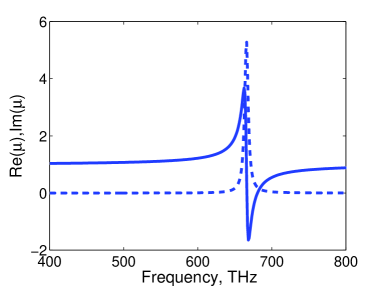
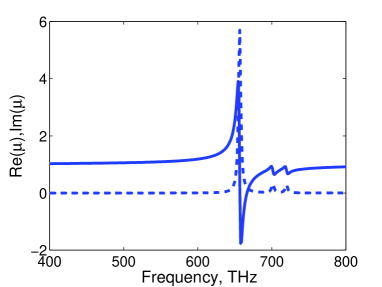
Figure 3: Effective permeability of the array of MNC with sizes $D_{p}=108$ nm, $a=22$ nm, $a_{p}=16$ nm ($R_{0}=38$ nm) hosted in the matrix with $\varepsilon_{h}=2.2$. 3: One ring of nanocolloids in every MNC, the concentration of MNC is $N_{MNC}=95^{-3}$ nm^-3. 3: Three nanorings in every MNC, other parameters are the same. Real and imaginary parts of the permeability are shown by solid and dashed lines, respectively.

The result for the effective permeability is presented in Fig. 3 (a). It reproduces Fig. 2 (b) of Engheta with high accuracy. This agreement can be considered as a check.

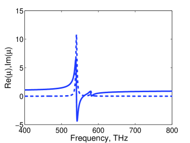
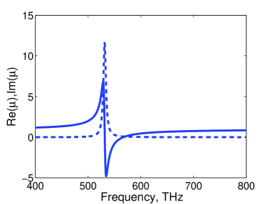
Figure 4: Effective permeability of the array of MNC with sizes $D_{p}=108$ nm, $a=22$ nm, $a_{p}=13$ nm, $d=6$ nm hosted in the matrix with $\varepsilon_{h}=2.2$, the concentration of MNC is $N_{MNC}=95^{-3}$ nm^-3. 5: First model of the interaction of nanocolloids. 5: Second model of the interaction of nanocolloids.

If we keep the same separation of colloidal particles $d=10$ nm as in the previous example the maximal possible number of colloidal particles for the spherical core of radius that corresponds to this example is equal to $N_{\rm tot}=16$. It corresponds to $N_{r}=3$. Keeping the same concentration $N_{MNC}=95^{-3}$ nm^-3 of same MNC we obtained with this geometry the result shown in Fig. 3 (b). This result was also obtained using the first model (for $N_{\rm tot}=16$ the second model is inadequate). The reduction of the magnetic resonance frequency due to the presence of two additional nanorings compared to Fig. 3 (a) is not dramatic though visible.

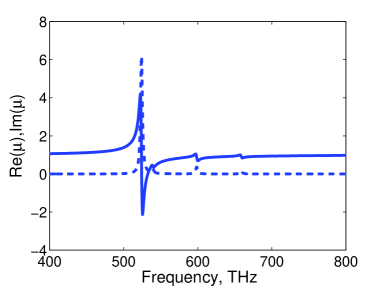
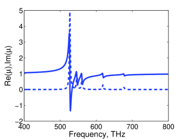
Figure 5: Effective permeability of the array of MNC with sizes $D_{p}=108$ nm, $a=22$ nm hosted in the matrix with $\varepsilon_{h}=2.2$, the concentration of MNC is $N_{MNC}=110$ nm^-3. 5: $a_{p}=13$ nm, $d=6$ nm. 5: $a_{p}=12.5$ nm, $d=6$ nm.

More promising results were obtained keeping the same total size of MNC $D_{p}=108$ nm for $a_{p}=13$ nm, $d=6$ nm, that implies $a=22$ nm. This geometry corresponds to one effective ring with $9$ colloids, two rings with $5$ colloids and two rings with $3$ colloids. In this case the number of colloidal particles is large enough and the qualitative agreement of two models was obtained. The concentration of MNC in Fig. 4 is the same as in the previous example: $N_{MNC}=95^{-3}$ nm^-3. The two models show approximately the same resonant frequency and the same magnitude of the resonance. The second model ignores, of course, the higher magnetic resonances that should arise in interacting nanorings and are revealed if we use the fist model. However, these higher resonances are weak and have no practical meaning.

The reduction of the resonant frequency in Fig. 4 compared to Fig. 3 means that the resonant size of the MNC reduces from $0.35\lambda_{r}$ as in the previous example to $0.25\lambda$ in the present one. Here $\lambda_{r}$ is the resonant wavelength in the host medium.

High magnitude of the Lorentz resonance in Fig. 4 means that we can also reduce the concentration of MNC making the array of MNC easier for manufacturing. The results depicted in Fig. 5 (a) and (b) are obtained using the first model for $N_{MNC}=110^{-3}$ nm^-3 instead of $N_{MNC}=95^{-3}$ nm^-3 as in the previous case. The difference between two plots in Fig. 5 (a) and (b) is determined by a 1 nm difference in the radiuses of plasmonic nanospheres, and demonstrates how sensible is the magnetic response of MNC to the deviation of parameters.

V Conclusions

In the present paper we developed the idea of the resonant optical magnetism in its isotropic variant modifying the known design of optical magnetic scatterers suggested in Engheta . The array of isotropic magnetic nanoclusters proposed in the present paper can be obtained in a liquid or porous matrix using the existing nanotechnologies. The metal nanocolloids are located in the core-shell particles attached to the silica core. Their electrostatic mutual coupling helps to reduce the resonant frequency for the given size of a nanocluster compared to the frequency of the plasmonic resonance of a single nanocolloid. This reduction is the essential result of the present paper since it allows one to decrease the spatial dispersion of the dense array (lattice) of nanoclusters. In other words, the suggested geometry is helpful for the isotropy of the effective resonant permeability of the array. The further optimization of the structure, further validation of the suggested model by full-wave numerical simulations are planned in the next paper.

References

- (1) N. Engheta, R. Ziolkowski, Metamaterials Physics and Engineering Explorations, NY: J. Wiley and Sons, 2006.
- (2) C. Caloz and T. Itoh, Electromagnetic Metamaterials: Transmission Line Theory and Microwave Applications. J. Wiley and Sons, NY, 2006.
- (3) Z. Liu, H. Lee, Y. Xiong, et al., Science 315, (2007) 1686.
- (4) I. I. Smolyaninov, Y.-J. Hung, C. C. Davis, et al., Sience 315 (2007) 1699.
- (5) V.A. Podolskiy, A.K. Sarychev and V.M. Shalaev, J. Nonlinear Opt. Phys. Mater. 11 (2002) 65.
- (6) A.K. Sarychev and V.M. Shalaev, in: Complex Medium V: Light and Complexity, Proc. SPIE 5508 (2004) 128.
- (7) A.K. Sarychev and V.M. Shalaev, in: negative Refraction Metamaterials: Fundamental Properties and Applications, G.V. Eleftheriades and K.G. Balmain Eds., Hoboken, NJ: John Wiley and Sons, 2005, 313.
- (8) G. Dolling, C. Enkrich, M. Wegener, et al., Opt. Lett. 30 (2005) 3198.
- (9) A.N. Grigorenko, A.K. Geim, H.F. Gleeson, et al., Nanofabricated media, Nature 438 (2005) 335.
- (10) S. Zhang, W. Fan, N.C. Panoiu, et al. Opt. Express 14 (2006) 6778.
- (11) G. Dolling, M. Wegener, and S. Linden, Opt. Lett. 32 (2007) 551.
- (12) C. Enkrich, M. Wegener, S. Linden, et al., Phys Rev. Lett. 95 (2005) 203901.
- (13) A.N. Serdyukov, I.V. Semchenko, S.A. Tretyakov, A. Sihvola, Electromagnetics of bi-anisotropic materials: Theory and applications, Amsterdam: Gordon and Breach Science Publishers, 2001.
- (14) A. Alú, A. Salandrino and N. Engheta, Optics Express 14 (2006) 1557.
- (15) K.C. Huang, M. L. Povinelli, and J.D. Joannopoulos, Applied Physics Letters 85 (2004) 543.
- (16) G. Shvets and Y. Urzhumov, Phys Rev. Lett. 93 (2004) 243902.
- (17) M.L. Povinelli, S. Johnson, J.D. Joannopoulos and J.B. Pendry, Appl. Phys. lett. 82 (2003) 1069.
- (18) M. Born and E. Wolf, Principles of Optics: Electromagnetic Theory of Propagation, Interference and Diffraction of Light, New York: Cambruidge University Press, 1999.
- (19) P. Drude, The Theory of Optics, 3d ed., London: Dover, 1959.
- (20) J. Li, G. Sun, C.T. Chan, Phys. rev. B, 73 (2003) 075117.
- (21) C.R. Simovski, Weak spatial dispersion in composite media, St. Petersburg: Politekhnika, 2003 (in Russian).
- (22) V.M. Agranovich, V.L. Ginzburg, Crystal optics with spatial dispersion and excitons, Berlin: Springer-Verlag, 1984.
- (23) S.J. Oldenburg, R.D. Averitt, S.L. Westcott, N.J. Halas, Chem Phys Lett, 288 (1998) 243.
- (24) S. Mornet, O. Lambert, E. Duguet, and A. Brisson, Nanoletters 5, 281-285 (2005)
- (25) L. Jiang, Z. Wu, D. Wu, et al., Nanotechnology 18 (2007) 185603.
- (26) S. Reculusa, C. Poncet-Legrand, S. Ravaine, et al., Chem. Mater., 14 (2002) 2354.
- (27) J.-C. Taveau, D. Nguyen, A. Perro, et al., Soft Matter, 4 (2008) 311.