Semileptonic hyperon decays in the self-consistent SU(3) chiral quark-soliton model

Abstract:

We investigate the semileptonic hyperon decays within the framework of the self-consistent SU(3) chiral quark-soliton model ($\chi$QSM). We take linear $1/N_{c}$ rotational as well as linear $m_{s}$ corrections into account and apply the symmetry conserving quantization. We present the results for the form factors $f_{1}(Q^{2})$, $f_{2}(Q^{2})$ and $g_{1}(Q^{2})$ in addition to the semileptonic decay constants of hyperons. We also have calculated the radii and dipole masses of these form factors for all relevant strangeness-conserving and strangeness-changing transitions.

1 Introduction

In the Standard model, the Cabibbo-Kobayashi-Maskawa matrix elements $|V_{ud}|$ and $|V_{us}|$ characterize the transition amplitudes for light hadron processes involving the quark transitions $d\to ue^{-}\overline{\nu}_{e}$ and $s\to ue^{-}\overline{\nu}_{e}$ [1, 2]. At present, the semileptonic kaon and $\pi^{+}$ decays [3, 4] provide the most precise measurement of the product $|V_{us}\cdot f_{+}(0)|$ with $f_{+}(0)$ being the kaon vector form factor. Generally, the Ademollo-Gatto theorem [5] states that the linear-order flavor $SU(3)$ breaking effects vanish in the vector matrix elements between hadron states in the same multiplet. This enables us to extract $V_{us}$ from kaon decays with high accuracy. On the other hand, the semileptonic hyperon decays (SHD) can be also used for an independent determination of $V_{us}$ and $V_{ud}$ [6, 7], where the product of $|V_{us}\cdot f_{1}(0)|$, $f_{1}(0)$ being the hyperon vector form factor, is accessed. Reference [6] has suggested to use recent experiments to compare the $V_{us}$ from the kaon with the SHD data.

Motivated by a recent progress in this field, we review in the present work the investigation of the semileptonic hyperon form factors in the chiral quark-soliton model ($\chi$QSM). Since the first results from the $\chi$QSM [8] on this issue, several new experimental and theoretical works have been developed. The KTeV collaboration first reported the measurement of the $\Xi^{0}\to\Sigma^{+}e^{-}\overline{\nu}_{e}$ decay [9] followed by the first determination of these form factors [10]. They published for this process the ratios $f_{2}(0)/f_{1}(0)=2.0\pm 1.2_{\textrm{stat}}\pm 0.5_{\textrm{syst}}$ and $g_{1}(0)/f_{1}(0)=1.32_{-0.17\textrm{stat}}^{+0.21}\pm 0.05_{\textrm{syst}}$. Very recently, the NA48/1 collaboration reported branching ratios for the same process with improved statistics, compared to the KTeV experiments, and announced $g_{1}(0)/f_{1}(0)=1.20\pm 0.05$ for $\Xi^{0}\to\Sigma^{+}e^{-}\overline{\nu}_{e}$ [11]. This particular SHD are interesting, since in flavor $SU(3)$ symmetry the $g_{1}/f_{1}$ ratio is equal to that of the neutron $\beta$ decay. The isospin partner process $\Xi^{-}\to\Sigma^{0}e^{-}\overline{\nu}$ was investigated in Ref. [12], where the ratio $g_{1}(0)/f_{1}(0)=1.25_{-0.16}^{+0.14}$ is presented together with the results for $\Lambda\to pe^{-}\overline{\nu}$ and $\Xi^{-}\to\Lambda e^{-}\overline{\nu}$. References [13, 14] invstigated $\Sigma^{-}\to\Lambda e^{-}\overline{\nu}$ as well as $\Lambda\to pe^{-}\overline{\nu}$.

On the theoretical side, chiral perturbation theory ($\chi$PT) is used to gain information about flavor $SU(3)$ breaking effects to $f_{1}(0)$ beyond the first order [15, 16, 17, 18], where other form factors of SHD have been also investigated. The results for $V_{us}$ and SHD data were discussed in Ref. [19] and for the large $N_{c}$ expansion in Ref. [20]. Very recently, Ref. [21] has also reported the first quenched lattice QCD study for all form factors of the $\Sigma^{-}\to nl\nu$ decay, in which the results were found to be: $f_{2}(0)/f_{1}(0)=-1.52\pm 0.81$ and $g_{1}(0)/f_{1}(0)=-0.287\pm 0.052$. In addition, Ref.[22] presents a study of SHD in a relativistic constituent quark model. We will see that our results are in qualitative agreement with these works as well as with the above mentioned experimental data.

In the present work we will investigate the vector $f_{1}(Q^{2})$, $f_{2}(Q^{2})$ and axial-vector $g_{1}(Q^{2})$ form factors for strangeness-conserving and strangeness-changing SHD in the self-consistent SU(3) $\chi$QSM. Since the form factors $f_{3}(Q^{2})$ and $g_{3}(Q^{2})$ are always multiplied by a factor of $m_{e}/M_{B}$ in the transition amplitude, they can be safely neglected. The value of the form factor $g_{2}(Q^{2})$ at $Q^{2}=0$ vanishes in exact SU(3) symmetry. Reference [8] presented in 1998 the SHD constants $f_{1}(0)$, $f_{2}(0)$ and $g_{1}(0)$ within the same framework of the $\chi$QSM. However, since then new experimental data as well as new theoretical results, some mentioned above, have been progressed and, moreover, Ref. [23] proposed in the $\chi$QSM the symmetry-conserving quantization that makes the Gell-Mann-Nishijima relation well satisfied. We extend, therefore, in this work the previous investigation to the full form factors up to $Q^{2}\leq 1\textrm{GeV}^{2}$ with the symmetry-conserving quantization employed [23]. We take into account linear $1/N_{c}$ rotational corrections as well as linear $m_{s}$ corrections.

A merit of the $\chi$QSM lies in the fact that we are able to calculate various unrelated baryonic observables within the same setting, once having determined the eigenvalues of the $\chi$QSM one-particle Dirac Hamiltonian. These eigenvalues were obtained by diagonalizing the Hamiltonian numerically with a self-consistent meson profile of the soliton, which is found in an action principle of minimizing the nucleon mass in the $\chi$QSM. The same eigenvalues were used in the past for investigating the mass splittings of the SU(3) baryons, form factors, and parton- and antiparton-distributions [24, 25, 26, 27, 28, 29, 30, 31, 32, 33, 34, 35], all relevant sum rules of these observables being simultaneously fulfilled. Nearly all observables are in good agreement with experimental data showing errors between $(10\sim 30)\,\%$. In particular, the dependence of all form factors on the momentum transfer is well reproduced within the $\chi$QSM. References [35, 36] have used the same set of fixed parameters as in the present work to investigate the strange electromagnetic form factors and the parity-violating asymmetries of polarized electron-proton scattering. In particular, the six electromagnetic form factors $G_{E,M}^{u,d,s}(Q^{2})$ and three axial-vector form factors $G_{A}^{u,d,s}(Q^{2})$ were calculated and are all in good agreement with experimental data. The vector and axial-vector form factors used in these $\chi$QSM-works are the basis for the present investigation. In addition, the same techniques were recently used for calculating observables of the anti-decuplet pentaquarks [37, 38]. The results describe well the experimental data avalilable so far, though their relevance is controversially discussed.

The present work is sketched as follows. In Section II, we present the general formalism for the SHD. In Section III, we show how to compute the observables of SHD within the selfconsistent SU(3) $\chi$QSM. In Section IV, we present and discuss the obtained results. In the final Section, we summarize the present work and draw conclusions. Additional detailed formulae are given in Appendices.

2 General Formalism

The decay rates for the SHD processes $B_{1}\to B_{2}l\overline{\nu}_{l}$ are determined by the transition matrix element $\mathcal{M}_{B_{1}\to B_{2}l\overline{\nu}_{l}}$ that is generally written as

$$\mathcal{M}_{B_{1}\to B_{2}l\overline{\nu}_{l}}=\frac{G_{F}}{\sqrt{2}}\,V\,\langle B_{2}|J_{W}^{\mu}|B_{1}\rangle\overline{u}_{l}(p_{l})\gamma_{\mu}(1-\gamma^{5})u_{\overline{\nu}_{l}}(p_{\nu}),$$ (1)

where $G_{F}$ denotes the well-known Fermi coupling constant and $V=V_{ud}(V_{us})$ stand for the Cabibbo-Kobayashi-Maskawa angles for $\Delta S=0$ ($\Delta S=1$) processes, respectively. It is the hadronic matrix element $\langle B_{2}|J_{W}^{\mu}|B_{1}\rangle$ that will be considered in this work for the $\Delta S=0$ transitions within the baryon octet:

$$n\to p,\,\,\,\,\,\,\,\,\,\,\Sigma^{-}\to\Lambda,\,\,\,\,\,\,\,\,\,\,\Sigma^{-}\to\Sigma^{0},\,\,\,\,\,\,\,\,\,\,\Xi^{-}\to\Xi^{0},\,\,\,$$ (2)

and $\Delta S=1$ transitions

$$\Sigma^{-}\to n,\,\,\,\,\,\,\,\,\,\,\Lambda\to p,\,\,\,\,\,\,\,\,\,\,\Xi^{-}\to\Sigma^{0},\,\,\,\,\,\,\,\,\,\,\Xi^{-}\to\Lambda.$$ (3)

All other transitions are related to these ones by isospin symmetry, of which the relations are given in the Appendix. The transition matrix elements for these two types of transitions are written explicitly as

$$\langle B_{2}(p_{2})|J_{W}^{\mu}(0)|B_{1}(p_{1})\rangle = \langle B_{2}(p_{2})|\overline{\psi}(0)\gamma^{\mu}(1-\gamma^{5})\frac{1}{2}\Big{(}\lambda^{1(4)}\pm i\lambda^{2(5)}\Big{)}\psi(0)|B_{1}(p_{1})\rangle,$$ (4)

where $\lambda^{\chi=1,2,4,5}$ are flavor SU(3) Gell-Mann matrices. Thus, we need to consider the following matrix elements for the vector current:

$$\langle B_{2}|J_{V}^{\mu\chi}|B_{1}\rangle = \langle B_{2}(p_{2})|\overline{\psi}(0)\gamma^{\mu}\frac{\lambda^{\chi}}{2}\psi(0)|B_{1}(p_{1})\rangle$$ (5)

$$= \overline{u}_{2}(p_{2})\Big{[}f_{1}^{B_{1}B_{2}}(Q^{2})\gamma^{\mu}+\frac{f_{2}^{B_{1}B_{2}}(Q^{2})i\sigma^{\mu\beta}q_{\beta}}{M_{B_{1}}}+\frac{f_{3}^{B_{1}B_{2}}(Q^{2})q^{\mu}}{M_{B_{1}}}\Big{]}\frac{\lambda^{\chi}}{2}u_{1}(p_{1}),$$ (6)

and for the axial-vector current:

$$\langle B_{2}|J_{A}^{\mu\chi}|B_{1}\rangle = \langle B_{2}(p_{2})|\overline{\psi}(0)\gamma^{\mu}\gamma^{5}\frac{\lambda^{\chi}}{2}\psi(0)|B_{1}(p_{1})\rangle$$ (7)

$$= \overline{u}_{2}(p_{2})\Big{[}g_{1}^{B_{1}B_{2}}(Q^{2})\gamma^{\mu}+\frac{g_{2}^{B_{1}B_{2}}(Q^{2})i\sigma^{\mu\beta}q_{\beta}}{M_{B_{1}}}$$ (9)

$$\hskip 170.71652pt+\;\frac{g_{3}^{B_{1}B_{2}}(Q^{2})q^{\mu}}{M_{B_{1}}}\Big{]}\gamma^{5}\frac{\lambda^{\chi}}{2}u_{1}(p_{1}),$$

where the form factors are normalized to the mass $M_{B_{1}}$ of the decaying particle. The form factors are known to be the real functions of the momentum-transfer $Q^{2}=-q^{2}$ with $q=p_{2}-p_{1}$. We concentrate on the form factors $f_{1}^{B_{1}B_{2}}(Q^{2})$, $f_{2}^{B_{1}B_{2}}(Q^{2})$ and $g_{1}^{B_{1}B_{2}}(Q^{2})$. The $f_{3}^{B_{1}B_{2}}(Q^{2})$, $g_{3}^{B_{1}B_{2}}(Q^{2})$ and $g_{2}^{B_{1}B_{2}}(Q^{2})$ are neglected since the first two are always suppressed by a factor of $(m_{e}/M_{B})^{2}$ due to $q^{\mu}$ in the cross section and the latter one is entirely due to the SU(3) symmetry breaking that is small for the octet baryons. We will first determine the SHD constants at $Q^{2}=0$ and the radii of these form factors for the transitions mentioned above. In order to calculate these form factors, we will use the rest frame of the decaying baryon $B_{1}$, i.e. $p_{1}=(M_{B_{1}},0)$, $p_{2}=(E_{2},{\bm{q}})$, where we have the kinematics

$${\bm{q}}^{2}=\Big{(}\frac{Q^{2}+M_{B_{1}}^{2}+M_{B_{2}}^{2}}{2M_{B_{1}}}\Big{)}^{2}-M_{B_{2}}^{2},\,\,\,\,\,\,\,\,\,\,\,\,E_{2}=\frac{Q^{2}+M_{B_{2}}^{2}+M_{B_{1}}^{2}}{2M_{B_{1}}}.$$ (10)

For the matrix element of the vector current given in Eq.(6), it is more convenient in the present scheme to calculate the Sachs-type form factors $G_{E}^{B_{1}B_{2}}(Q^{2})$ and $G_{M}^{B_{1}B_{2}}(Q^{2})$, since they are directly related to the matrix elements of the time and space components of the vector current as follows:

$$G_{E}^{B_{1}B_{2}}(Q^{2}) = \int\frac{d\Omega_{q}}{4\pi}\langle B_{2}(p_{2})|J_{V}^{0}(0)|B_{1}(p_{1})\rangle,$$ (11)

$$G_{M}^{B_{1}B_{2}}(Q^{2}) = 3M_{p}\int\frac{d\Omega_{q}}{4\pi}\frac{q^{i}\epsilon^{ik3}}{i\mid{\bm{q}}\mid^{2}}\langle B_{2}(p_{2})|J_{V}^{k}(0)|B_{1}(p_{1})\rangle,$$ (12)

where $G_{M}^{B_{1}B_{2}}(Q^{2})$ is multiplied by the proton mass $M_{p}$. This gives in the rest frame of $B_{1}$ by explicitly applying those projections to the right-hand side of Eq.(6) for equal initial and final baryon spins:

$$G_{E}^{B_{1}B_{2}}(Q^{2}) = Nf_{1}^{B_{1}B_{2}}(Q^{2})-f_{2}^{B_{1}B_{2}}(Q^{2})\frac{1}{M_{B_{1}}}\frac{N{\bm{q}}^{2}}{E_{2}+M_{B_{2}}}+f_{3}^{B_{1}B_{2}}(Q^{2})\frac{q^{0}}{M_{B_{1}}}N,$$ (13)

$$G_{M}^{B_{1}B_{2}}(Q^{2}) = \frac{2M_{p}N}{E_{2}+M_{B_{2}}}\Big{[}f_{1}^{B_{1}B_{2}}(Q^{2})+f_{2}^{B_{1}B_{2}}(Q^{2})\frac{M_{B_{1}}+M_{B_{2}}}{M_{B_{1}}}\Big{]}$$ (14)

with $N=\sqrt{(E_{2}+M_{B_{2}})/(2M_{B_{2}})}$. The $M_{B_{1}}$ in the denominator comes from the normalization of $f_{2}^{B_{1}B_{2}}(Q^{2})$ and $f_{3}^{B_{1}B_{2}}(Q^{2})$. The operators applied on the time and space components of the vector current in Eqs.(11,12) are the same that project out the normal Sachs form factors $G_{E}(Q^{2})$, $G_{M}(Q^{2})$ in the case of, e.g., the proton electric and magnetic form factors.

In order to extract the form factors $g_{1}^{B_{1}B_{2}}(Q^{2})$, it is helpful to contract the spacial component of the current in Eq.(9), multiplying by ${\bm{q}}\times({\bm{q}}\times$, and to perform afterwards the average over the orientation of the angular momentum. Choosing the initial and final baryon-spins to be equal, we extract $g_{1}^{B_{1}B_{2}}(Q^{2})$ from the third spacial component.

$$\int\frac{d\Omega_{q}}{4\pi}{\bm{q}}\times\Big{(}{\bm{q}}\times\langle B_{2}(p_{2})|{\bm{J}}_{A}(0)|B_{1}(p_{1})\rangle\Big{)}=Ng_{1}^{B_{1}B_{2}}(Q^{2})(-)\frac{2}{3}\,{\bm{q}}^{2}\phi_{s^{2}}^{\dagger}{\bm{\sigma}}\phi_{s^{1}},$$ (15)

$$g_{1}^{B_{1}B_{2}}(Q^{2})=\frac{1}{N}(-)\frac{3}{2}\frac{1}{{\bm{q}}^{2}}\int\frac{d\Omega_{q}}{4\pi}{\bm{q}}\times\Big{(}{\bm{q}}\times\langle B_{2}(p_{2})|{\bm{J}}_{A}(0)|B_{1}(p_{1})\rangle\Big{)}_{z}.$$ (16)

3 The Form factors in the Chiral Quark-Soliton Model

In this Section, we show briefly how to compute Eqs.(11,12,16) in the SU(3) $\chi$QSM. For details we refer to Ref. [24, 40, 39, 41]. In general, the baryonic matrix elements are expressed by

$$\langle B_{2}(p_{2})|\mathcal{J}^{\mu\chi}(0)|B_{1}(p_{1})\rangle=\langle B_{2}(p_{2})|\overline{\psi}(0)\mathcal{O}^{\mu\chi}\psi(0)|B_{1}(p_{1})\rangle,$$ (17)

where the explicit form of $\mathcal{O}^{\mu\chi}$ are found in Eqs.(11,12,16). In order to evaluate the matrix elements in the model, we start from the low-energy effective partition function defined as follows:

$$\mathcal{Z}_{\mathrm{\chi QSM}}=\int\mathcal{D}\psi\mathcal{D}\psi^{\dagger}\mathcal{D}U\exp\left[-\int d^{4}x\psi^{\dagger}iD(U)\psi\right]=\int\mathcal{D}U\exp(-S_{\mathrm{eff}}[U]),$$ (18)

where $\psi$ and $U$ denote the quark and pseudo-Goldstone boson fields, respectively. The $S_{\mathrm{eff}}$ stands for the effective chiral action expressed as

$$S_{\mathrm{eff}}(U)=-N_{c}\mathrm{Tr}\ln iD(U),$$ (19)

where $\mathrm{Tr}$ represents the functional trace, $N_{c}$ the number of colors, and $D$ the Dirac differential operator in Euclidean space:

$$D(U)=\gamma^{4}(i\hbox to0.0pt{/\hss}{\partial}-\hat{m}-MU^{\gamma_{5}})=-i\partial_{4}+h(U)-\delta m.$$ (20)

We assume isospin symmetry and decompose the current quark mass matrix into $\hat{m}=\mathrm{diag}(\overline{m},\,\overline{m},\,m_{\mathrm{s}})=\overline{m}+\delta m$ with $\overline{m}$ and $m_{s}$ as the average of the up- and down-quark masses and strange quark mass, respectively. The $\delta m$ is given by

$$\delta m=M_{1}\gamma^{4}\bm{1}+M_{8}\gamma^{4}\lambda^{8},$$ (21)

where $M_{1}$ and $M_{8}$ are singlet and octet components of the current quark masses defined as $M_{1}=(-\overline{m}+m_{\mathrm{s}})/3$ and $M_{8}=(\overline{m}-m_{\mathrm{s}})/\sqrt{3}$. The $\partial_{4}$ designates the derivative with respect to the Euclidean time and $h(U)$ stands for the Dirac single-quark Hamiltonian:

$$h(U)=i\gamma^{4}\gamma^{i}\partial_{i}-\gamma^{4}MU^{\gamma_{5}}-\gamma^{4}\overline{m}.$$ (22)

For the chiral field $U^{\gamma_{5}}$, we assume Witten’s embedding of the SU(2) soliton into SU(3)

$$U_{\mathrm{SU(3)}}=\left(\begin{array}[]{lr}U_{\mathrm{SU(2)}}&0\\ 0&1\end{array}\right)$$ (23)

with the SU(2) pion field $\pi(x)$ as

$$U^{\gamma_{5}}=\exp(i\gamma^{5}\tau^{i}\pi^{i}(x))=\frac{1+\gamma^{5}}{2}U+\frac{1-\gamma^{5}}{2}U^{\dagger}.$$ (24)

The integration over the pion field in Eq.(18) can be done by using the saddle-point approximation in the large $N_{c}$ limit due to the $N_{c}$ factor in Eq.(19). In order to find the pion field that minimizes the action in Eq.(19) and to calculate Eq.(17), we make the following Ansätze. The SU(2) pion field $U$ has the most symmetric form known as the hedgehog form:

$$U_{\mathrm{SU2}}=\exp[i\gamma_{5}\hat{\bm{n}}\cdot\bm{\tau}P(r)],$$ (25)

where $P(r)$ is the radial pion profile function.

The baryon state is defined as an Ioffe-type current consisting of $N_{c}$ valence quarks [24]:

$$|B(p)\rangle = \lim_{x_{4}\to-\infty}\,\frac{1}{\sqrt{\mathcal{Z}}}\,e^{ip_{4}x_{4}}\,\int d^{3}{\bm{x}}\,e^{i\,{\bm{p}}\cdot{\bm{x}}}\,J_{B}^{\dagger}(x)\,|0\rangle,$$ (26)

$$J_{B}(x) = \frac{1}{N_{c}!}\,\Gamma_{B}^{b_{1}\cdots b_{N_{c}}}\,\varepsilon^{\beta_{1}\cdots\beta_{N_{c}}}\,\psi_{\beta_{1}b_{1}}(x)\cdots\psi_{\beta_{N_{c}}b_{N_{c}}}(x),$$ (27)

where the matrix $\Gamma_{B}^{b_{1}...b_{N_{c}}}$ carries the hyper-charge $Y$, isospin $I,I_{3}$ and spin $J,J_{3}$ quantum numbers of the baryon. The $b_{i}$ and $\beta_{i}$ denote the spin-flavor- and color-indices, respectively. Thus, we can write the baryonic matrix element of the quark current $\mathcal{J}^{\mu\chi}$ as follows:

$$\langle B_{2}(p_{2})|\mathcal{J}^{\mu\chi}(0)|B_{1}(p_{1}\rangle = \frac{1}{\mathcal{Z}}\lim_{T\to\infty}e^{-ip_{2}^{4}\frac{T}{2}+ip_{1}^{4}\frac{T}{2}}\int d^{3}{\bm{x}}^{\prime}d^{3}{\bm{x}}e^{i{\bm{p}}_{1}\cdot{\bm{x}}-i{\bm{p}}_{2}\cdot{\bm{x}}^{\prime}}$$ (28)

$$\times \int\mathcal{D}U\mathcal{D}\psi^{\dagger}\mathcal{D}\psi J_{B^{\prime}}\left(\frac{T}{2},{\bm{x}}^{\prime}\right)\mathcal{J}^{\mu\chi}(0)J_{B}^{\dagger}\left(-\frac{T}{2},{\bm{x}}\right)$$ (30)

$$\times\exp{\left[-\int d^{4}x\,\psi^{\dagger}iD(U)\psi\right]}.$$

Taking $\mathcal{J}^{\mu\chi}(0)=1$ in Eq.(30), we get the nucleon correlation function from which we can obtain the expression for the classical nucleon mass in the limit of $T\to\infty$. The self-consistent soliton profile $P_{c}(r)$ in the saddle-point approximation is found by minimizing the nucleon mass in the $\chi$QSM, i.e., by solving numerically the equation of motion coming from $\delta S_{eff}/\delta P(r)=0$.

Since the soliton does not have good quantum numbers for rotations as well as translations, we need to quantize it. This can by done by the zero-mode quantization as follows:

$$U(\bm{x},t)=A(t)U_{c}(\bm{x}-\bm{z}(t))A^{\dagger}(t),$$ (31)

where $A(t)$ denotes a unitary time-dependent SU(3) collective orientation matrix and $\bm{z}(t)$ stands for the time-dependent translation of the center of mass of the soliton in coordinate space. A detailed formalism can be found in Refs.[24, 39]. Taking the zero-modes into account, we find the Dirac operator in Eq.(20) in the following form:

$$D(U)=T_{z(t)}A(t)\left[D(U_{c})+i\Omega(t)-\dot{T}_{z(t)}^{\dagger}T_{z(t)}-i\gamma^{4}A^{\dagger}(t)\delta mA(t)\right]T_{z(t)}^{\dagger}A^{\dagger}(t),$$ (32)

where the $T_{z(t)}$ denotes the translational unitary operator and the $\Omega(t)$ represents the soliton angular velocity defined as

$$\Omega=-iA^{\dagger}\dot{A}=-\frac{i}{2}\textrm{Tr}(A^{\dagger}\dot{A}\lambda^{\alpha})\lambda^{\alpha}=\frac{1}{2}\Omega_{\alpha}\lambda^{\alpha}.$$ (33)

Assuming that the soliton rotates and moves slowly, we can treat the $\Omega(t)$ and $\dot{T}_{z(t)}^{\dagger}T_{z(t)}$ perturbatively. Moreover, the strange current quark mass $\hat{m}$ is regarded as a small parameter, so that we also deal with $\delta m$ perturbatively. The collective baryon wavefunction on the level of Eq.(30) is then introduced as

$$\psi_{(\mathcal{R}^{*};Y^{\prime}JJ_{3})}^{(\mathcal{R};YII_{3})}(A):=\lim_{T\mapsto\infty}\frac{1}{\sqrt{\mathcal{Z}}}e^{-p^{4\prime}T/2}\int d^{3}{\bm{u}}^{\prime}e^{i{\bm{p}}^{\prime}\cdot{\bm{u}}^{\prime}}(\Gamma_{B}^{b_{1}...b_{N_{c}}})^{*}\Pi_{l=1}^{N_{c}}\big{[}\varphi^{\dagger}_{v,b_{l}}({\bm{u}}^{\prime})A^{\dagger}\big{]}.$$ (34)

Having expanded and quantized the soliton, we obtain the following collective Hamiltonian [42]:

$$H_{\textrm{coll}}=H_{\mathrm{sym}}+H_{\mathrm{sb}}\,\,\,,$$ (35)

where $H_{\mathrm{sym}}$ and $H_{\mathrm{sb}}$ represent the SU(3) symmetric and symmetry-breaking parts, respectively:

$$H_{\mathrm{sym}} = M_{c}+\frac{1}{2I_{1}}\sum_{i=1}^{3}J_{i}J_{i}+\frac{1}{2I_{2}}\sum_{a=4}^{7}J_{a}J_{a},$$ (36)

$$H_{\mathrm{sb}} = \frac{1}{\overline{m}}M_{1}\Sigma_{SU(2)}+\alpha D_{88}^{(8)}(A)+\beta Y+\frac{\gamma}{\sqrt{3}}D_{8i}^{(8)}(A)J_{i}.$$ (37)

The $M_{c}$ denotes the mass of the classical soliton and $I_{i}$ and $K_{i}$ are the moments of inertia of the soliton [24], of which the corresponding expressions can be found in Ref. [43] explicitly. The components $J_{i}$ denote the spin generators and $J_{a}$ correspond to those of right rotations in flavor SU(3) space. The $\Sigma_{\mathrm{SU(2)}}$ is the SU(2) pion-nucleon sigma term. The $D_{88}^{(8)}(A)$ and $D_{8i}^{(8)}(A)$ stand for the SU(3) Wigner $D$ functions in the octet representation. The $Y$ is the hypercharge operator. The parameters $\alpha$, $\beta$, and $\gamma$ in the symmetry-breaking Hamiltonian are expressed, respectively, as follows:

$$\alpha=\frac{1}{\overline{m}}\frac{1}{\sqrt{3}}M_{8}\Sigma_{SU(2)}-\frac{N_{c}}{\sqrt{3}}M_{8}\frac{K_{2}}{I_{2}},\;\;\;\;\beta=M_{8}\frac{K_{2}}{I_{2}}\sqrt{3},\;\;\;\;\gamma=-2\sqrt{3}M_{8}\left(\frac{K_{1}}{I_{1}}-\frac{K_{2}}{I_{2}}\right).$$ (38)

The collective wavefunctions of the Hamiltonian in Eq.(35) can be found as the SU(3) Wigner $D$ functions in representation $\mathcal{R}$:

$$\langle A|\mathcal{R},B(YII_{3},Y^{\prime}JJ_{3})\rangle=\Psi_{(\mathcal{R}^{*};Y^{\prime}JJ_{3})}^{(\mathcal{R};YII_{3})}(A)=\sqrt{\textrm{dim}(\mathcal{R})}\,(-)^{J_{3}+Y^{\prime}/2}\,D_{(Y,I,I_{3})(-Y^{\prime},J,-J_{3})}^{(\mathcal{R})*}(A).$$ (39)

The $Y^{\prime}$ is related to the eighth component of the angular velocity $\Omega$ that is due to the presence of the discrete valence quark level in the Dirac-sea spectrum. Its presence has no effect on the chiral field, so that it is constrained to be $Y^{\prime}=-N_{c}/3=-1$. In fact, this constraint allows us to have only the SU(3) representations with zero triality.

Due to flavor SU(3) symmetry breaking the collective baryon states are not in a pure representation but get mixed with other representations. This can be treated by first-order perturbation for the collective Hamiltonian:

$$|B_{\mathcal{R}}\rangle=|B_{\mathcal{R}}^{\mathrm{sym}}\rangle-\sum_{\mathcal{R}^{\prime}\neq\mathcal{R}}|B_{\mathcal{R}^{\prime}}\rangle\frac{\langle B_{\mathcal{R}^{\prime}}|\,H_{\textrm{sb}}\,|B_{\mathcal{R}}\rangle}{M(\mathcal{R}^{\prime})-M(\mathcal{R})}\,.$$ (40)

Solving Eq.(40), we obtain the collective wavefunctions for the baryon octet:

$$|B_{8}\rangle=|8_{1/2},B\rangle+c_{\overline{10}}^{B}|\overline{10}_{1/2},B\rangle+c_{27}^{B}|27_{1/2},B\rangle,$$ (41)

where the mixing coefficients $c_{\overline{10}}^{B}$ and $c_{27}^{B}$ are defined as

$$c_{\overline{10}}^{B}=c_{10}\,\Big{[}\sqrt{5},0,\sqrt{5},0\Big{]},\,\,\,\,\,\,\,\,\,\,c_{27}^{B}=c_{27}\,\Big{[}\sqrt{6},3,2,\sqrt{6}\Big{]}$$ (42)

in the basis $[N,\Lambda,\Sigma,\Xi]$ with

$$c_{\overline{10}}=-\frac{I_{2}}{15}\Big{(}\alpha+\frac{1}{2}\gamma\Big{)},\,\,\,\,\,\,\,\,\,\,c_{27}=-\frac{I_{2}}{25}\Big{(}\alpha-\frac{1}{6}\gamma\Big{)}.$$ (43)

We are now in a position to evaluate the baryonic matrix elements such as Eq.(17), i.e. to solve Eq.(30) with a certain expression of $\mathcal{J}^{\mu\chi}(0)$ given. We have now the general expression for the baryonic matrix elements as follows:

$$\langle B_{2}(p_{2})|\psi^{\dagger}(0)\mathcal{O}^{\mu\chi}\psi(0)|B_{1}(p_{1})\rangle=\int dA\int d^{3}z\,\,e^{i{\bm{q}}\cdot{\bm{z}}}\Psi_{B_{2}}^{*}(A)\mathcal{G}^{\mu\chi}({\bm{z}})\Psi_{B_{1}}(A)e^{S_{eff}},$$ (44)

where $dA$ and $d^{3}z$ arise from the zero-mode quantizations and the expression $\mathcal{G}^{\mu\chi}({\bm{z}})$ contains the specific form factor parts. We have used again the saddle-point approximation and expanded the Dirac operator with respect to $\Omega$ and $\delta m$ to the linear order and $\dot{T}_{z(t)}^{\dagger}T_{z(t)}$ to the zeroth order. Defining $\mathcal{J}^{\mu\chi}(0)$ and contracting the Lorentz index in Eq.(44) according to Eqs.(11,12,16), we get the final expressions in the $\chi$QSM for the vector form factors as follows:

$$G_{E}^{\chi}(Q^{2}) = \int d^{3}z\,j_{0}(|{\bm{q}}||{\bm{z}}|)\,\langle B_{2}|\mathcal{G}_{E}^{\chi}({\bm{z}})|B_{1}\rangle,$$ (45)

$$G_{M}^{\chi}(Q^{2}) = M_{p}\int d^{3}z\frac{j_{1}(|{\bm{q}}||{\bm{z}}|)}{|{\bm{q}}||{\bm{z}}|}\,\langle B_{2}|\mathcal{G}_{M}^{\chi}({\bm{z}})|B_{1}\rangle,$$ (46)

and axial-vector form factors as

$$g_{1}^{\chi}(Q^{2})=\int d^{3}z\,\Big{[}j_{0}(|{\bm{z}}||{\bm{q}}|)\,\langle B_{2}|\mathcal{G}_{10}^{\chi}({\bm{z}})|B_{1}\rangle-\sqrt{2\pi}j_{2}(|{\bm{z}}||{\bm{q}}|)\,\langle B_{2}|\{Y_{2}\otimes\mathcal{G}_{1}^{\chi}({\bm{z}})\}_{10}|B_{1}\rangle\Big{]},$$ (47)

where $j_{0,1,2}$ denote the spherical Bessel functions. The expressions $\mathcal{G}_{E}^{\chi}({\bm{z}})$, $\mathcal{G}_{M}^{\chi}({\bm{z}})$ and $\mathcal{G}_{10}^{\chi}({\bm{z}}),\{Y_{2}\otimes\mathcal{G}_{1}^{\chi}({\bm{z}})\}_{10}$ can be found in Appendix A. The expansion in $\Omega$ and $\delta m$ provides the following structure of the form factor structure:

$$G^{B_{1}B_{2}}_{E,M,A}(Q^{2}) = G_{E,M,A}^{(\Omega^{0},m_{s}^{0})}(Q^{2})+G_{E,M,A}^{(\Omega^{1},m_{s}^{0})}(Q^{2})+G_{E,M,A}^{(m_{s}^{1}),\textrm{op}}(Q^{2})+G_{E,M,A}^{(m_{s}^{1}),\textrm{wf}}(Q^{2}),$$ (48)

where the first term corresponds to the leading order ($\Omega^{0},m_{s}^{0}$), the second one to the first $1/N_{c}$ rotational corrections ($\Omega^{1},m_{s}^{0}$), the third to the linear $m_{s}$ corrections coming from the operator, and the last one to the wavefunction corrections, respectively.

In the whole approach we take only orders of $\mathcal{O}(m_{s}^{0})$ and $\mathcal{O}(m_{s}^{1})$ into account for the expression $\mathcal{G}^{\mu\chi}$ and consider only the zeroth order $\mathcal{O}(m_{s}^{0})$ for the expression $e^{i{\bm{q}}\cdot{\bm{z}}}$ in Eq.(44). In the $\chi$QSM, we may write the masses $M_{B_{2}}$ of the baryon octet as

$$M_{B_{2}}=M_{B_{1}}+\textrm{const}\cdot m_{s}$$ (49)

with $M_{B_{1}}\sim\mathcal{O}(N_{c})$, so that the second term is of order $\mathcal{O}(N_{c}^{0},m_{s}^{1})$. Inserting Eq.(49) in the definition of the momentum transfer in Eq.(10) and neglecting all terms of higher order than $\mathcal{O}(m_{s}^{0})$, we get

$${\bm{q}}^{2}\stackrel{{\scriptstyle N_{c}\to\infty}}{{=}}Q^{2},$$ (50)

which means that for each transition form factor the momentum dependence turns out to be

$$j_{0,1,2}(|{\bm{q}}||{\bm{z}}|)\to j_{0,1,2}(\sqrt{Q^{2}}|{\bm{z}}|)\,\,\,.$$ (51)

In order to get the baryonic matrix element in the form of Eq.(44), we have used the large $N_{c}$ limit. Taking also the limit of $N_{c}\to\infty$ on the RHS of Eqs.(13,14), we obtain the following relations:

$$E_{B} = M_{B}+\frac{{\bm{p}}}{2M_{B}}+\mathcal{O}(N_{c}^{-2}),$$ (52)

$$\sqrt{\frac{E_{B}+M_{B}}{2M_{B}}} = 1+\mathcal{O}(N_{c}^{-2}),$$ (53)

$$\frac{1}{M_{B_{1}}}\frac{N{\bm{q}}^{2}}{E_{2}+M_{B_{2}}} = \mathcal{O}(N_{c}^{-2})+\mathcal{O}(N_{c}^{-1},m_{s}^{1}),$$ (54)

$$\frac{q^{0}}{M_{B_{1}}}N = \mathcal{O}(N_{c}^{-2})+\mathcal{O}(N_{c}^{-1},m_{s}^{1}),$$ (55)

$$\frac{2M_{p}N}{E_{2}+M_{B_{2}}} = \frac{2M_{p}(1+\mathcal{O}(N_{c}^{-2}))}{2M_{B_{2}}(1+\mathcal{O}(N_{c}^{-2}))}=\frac{M_{p}}{M_{B_{2}}},$$ (56)

so that the vector form factors calculated in the $\chi$QSM via Eqs.(45,46) corresponds to

$$G_{E}^{B_{1}B_{2}}(Q^{2}) = f_{1}^{B_{1}B_{2}}(Q^{2})$$ (57)

$$G_{M}^{B_{1}B_{2}}(Q^{2}) = \frac{M_{p}}{M_{B_{2}}}\Big{[}f_{1}^{B_{1}B_{2}}(Q^{2})+f_{2}^{B_{1}B_{2}}(Q^{2})\frac{M_{B_{1}}+M_{B_{2}}}{M_{B_{1}}}\Big{]}.$$ (58)

The factor of $1/N$ in Eq.(16) reduces to $1$ because of the same arguments.

In the $\chi$QSM Hamiltonian of Eq.(22), the constituent quark mass $M$ is the only free parameter and $M=420\,\textrm{MeV}$ is known to reproduce very well experimental data [29, 40, 35, 39]. Though the $M=420$ MeV yields the best results for the baryon octet, we will present also those for $M=400\,\textrm{MeV}$ and $M=450\,\textrm{MeV}$ to see the $M$ dependence of the results in this work. Throughout this work the strange current quark mass is fixed to $m_{\mathrm{s}}=180\,\textrm{MeV}$. In order to tame the divergent quark loops, we employ in this work the proper-time regularization. The cut-off parameter and $\overline{m}$ are fixed for a given $M$ to the pion decay constant $f_{\pi}$ and $m_{\pi}$, respectively. The numerical results for the moments of inertia and mixing coefficients are summarized in Table 1 for $M=420$ MeV.

Table 1: Moments of inertia and mixing coefficients for $M=420\,\textrm{MeV}$.

$I_{1}\,[\textrm{fm}]$	$I_{2}\,[\textrm{fm}]$	$K_{1}\,[\textrm{fm}]$	$K_{2}\,[\textrm{fm}]$	$\Sigma_{\pi N}\,[\textrm{MeV}]$	$c_{\overline{10}}$	$c_{27}$
$1.06$	$0.48$	$0.42$	$0.26$	$41$	$0.037$	$0.019$

The results in Table 1 are obtained with the same parameters used in previous works [35, 44, 45]. We want to emphasize that all model parameters are the same as before. In previous works, the axial-vector form factors for the nucleon were already calculated. The axial-vector constants $g_{A}^{3},g_{A}^{8}$ were found to be $g_{A}^{3}=1.176$ and $g_{A}^{8}=0.36$ which is in very good agreement with experimental data $g_{A}^{3}=1.267\pm 0.0029$ [46] and $g_{A}^{8}=0.338\pm 0.15$ [47]. With these numerical parameters, the $\chi$QSM yields the masses of the octet baryons in unit of MeV as Ref. [38]:

$$M_{N}=1001(939),\,\,\,\,M_{\Lambda}=1124(1116),\,\,\,\,M_{\Sigma}=1179(1189),\,\,\,\,M_{\Xi}=1275(1318),$$ (59)

where the numbers in the parentheses are the experimental values of the Particle Data Group [46]. The $\chi$QSM values were obtained by first calculating the hyper-charge splittings with Eq.(35) and using the experimental octet mass center of $M_{8}=(M_{\Lambda}+M_{\Sigma})/2=1151.5$MeV.

4 Results and Discussion

In the present work, we consider linear $m_{s}$ corrections. According to the Ademollo-Gatto theorem [5] SU(3) symmetry-breaking effects contribute to the matrix elements of the vector current between the states in the same SU(3) multiplet earliest at second order in $m_{s}$. Since we restrict ourselves in the present investigation to first order in $m_{s}$, we have for $f_{1}^{B_{1}B_{2}}(0)$ only the SU(3) symmetric results. The SHD constants in the $\chi$QSM were already investigated in Ref. [8]. The constants of $g_{1}(0)/f_{1}(0)$ were also discussed in the $\chi$QSM formulated in a Fock representation on the light cone [48]. In the present work we will extend the earlier work [8] by considering the full form factors of $f_{1}(Q^{2})$, $f_{2}(Q^{2})$ and $g_{1}(Q^{2})$ up to $Q^{2}\leq 1\textrm{GeV}^{2}$ and also taking into account the symmetry-conserving quantization. The symmetry-conserving quantization was found after the publication of Ref. [8] and does also have effects on the SHD constants.

4.1 SHD vector form factors

We now present the results for the vector transition form factors $f^{B_{1}B_{2}}_{1}(Q^{2})$ and $f^{B_{1}B_{2}}_{2}(Q^{2})$ in the $\chi$QSM, for which we have the following relations from Eq.(57):

$$f_{1}^{B_{1}B_{2}}(Q^{2})=G_{E}^{B_{1}B_{2}}(Q^{2}),\,\,\,\,\,\,\,\,\,\,\,\,\,f_{2}^{B_{1}B_{2}}(Q^{2})=\frac{M_{B_{1}}}{M_{B_{1}}+M_{B_{2}}}\Big{[}G_{M}^{B_{1}B_{2}}(Q^{2})\frac{M_{B_{2}}}{M_{p}}-f_{1}^{B_{1}B_{2}}(Q^{2})\Big{]}.$$ (60)

We first discuss the results of the SHD constants at $Q^{2}=0$. Due to the expressions

$$\int d^{3}z\,\mathcal{B}({\bm{z}})=3,\;\;\;\frac{1}{I_{i}}\int d^{3}z\,\mathcal{I}_{i}({\bm{z}})=1,\;\;\;\frac{1}{K_{i}}\int d^{3}z\,\mathcal{K}_{i}({\bm{z}})=1,\;\;\;\int d^{3}z\,\mathcal{C}({\bm{z}})=0,$$ (61)

we see that Eq.(45) with Eq.(81) and the corresponding coefficients in Appendix C give the following values:

$$f_{1}^{np}(0)=1, f_{1}^{\Sigma^{-}n}(0)=1,$$ (62)

$$f_{1}^{\Sigma^{-}\Lambda}(0)=0, f_{1}^{\Lambda p}(0)=\sqrt{\frac{3}{2}},$$ (63)

$$f_{1}^{\Sigma^{-}\Sigma^{0}}(0)=\sqrt{2}, f_{1}^{\Xi^{-}\Sigma^{0}}(0)=\frac{1}{\sqrt{2}},$$ (64)

$$f_{1}^{\Xi^{-}\Xi^{0}}(0)=1, f_{1}^{\Xi^{-}\Lambda}(0)=\sqrt{\frac{3}{2}}.$$ (65)

Since we only take linear $m_{s}$ corrections into account the $m_{s}$ corrections both from the operator and from the wavefunction add up to zero at $Q^{2}=0$ which is the consequence of the Ademollo-Gatto theorem.

In the case of the SHD constants $f_{2}(0)$, Eq.(46) for $G_{M}^{B_{1}B_{2}}(0)$ is involved. This expression contains explicitly a factor of $M_{p}$. The proton mass in the $\chi$QSM turns out to be $1.36$ times larger than the experimental proton mass, i.e. $M_{p}^{\chi\mathrm{QSM}}=1.36M_{p}^{\mathrm{exp}}$. This is a well understood property of the $\chi\mathrm{QSM}$ [49], whose consequences we cure as usual in the following way. We will calculate Eq.(46), which is a pure model expression, with the soliton-nucleon mass. However, having determined the $G_{M}^{B_{1}B_{2}}(0)$, we will then use experimental values for further calculations, such as calculating $f_{2}^{B_{1}B_{2}}(0)$ in Eq.(60). The used experimental masses are given in units of GeV as follows:

$$M_{p}=M_{N}=0.939, M_{\Lambda}=1.116,$$ (66)

$$M_{\Sigma}=1.186, M_{\Xi}=1.318.$$ (67)

Results for the constants $f_{1}^{B_{1}B_{2}}(0)$, $G_{M}^{B_{1}B_{2}}(0)$ and $f_{2}^{B_{1}B_{2}}(0)$ are given in Table 2 for the constituent quark mass of $M=420$MeV. We find that the constants are not sensitive to $M$. In Ref.[8] it was found that linear $m_{s}$ corrections to the form factor $f_{2}$ are sizable for some transitions, explicitly for the transitions $\Sigma^{-}\to\Sigma^{0}$ and $\Xi^{-}\to\Sigma^{0}$. Due to the application of the symmetry-conserving quantization the absolute values of the transition constants are changing but the effects of the $m_{s}$ corrections on this work are comparable to those in Ref. [8]. In the case of $G_{M}(0)$, we have used the soliton-nucleon mass in Eq.(58), while we have employed experimental masses for Eq.(60).

Table 2: Results for $f_{1}^{B_{1}B_{2}}(0)$, $G_{M}^{B_{1}B_{2}}(0)$ and $f_{2}^{B_{1}B_{2}}(0)$ in the self-consistent $\chi$QSM for the constituent quark mass of $420$ MeV. We show the results with and without linear $m_{s}$ corrections. The SHD constants $f_{1}^{B_{1}B_{2}}(0)$ do not acquire any linear $m_{s}$ corrections. The superscript $[\mathrm{SU(3)}]$ indicates the SU(3) symmetry conserving approximation. The final results are given in the column $f_{1}(0)$ and in the columns with superscript $[m_{s}^{0}+m_{s}^{1}]$. The $SU(3)$ anomalous magnetic moments of the nucleons in the $\chi$QSM are obtained as $\kappa_{p}=1.47$ and $\kappa_{n}=-1.64$.

	$G_{M}^{\mathrm{SU(3)}}(0)$	$G_{M}^{m_{s}^{0}+m_{s}^{1}}(0)$	$f_{1}(0)$	$f_{2}^{\mathrm{SU(3)}}(0)$	$f_{2}^{m_{s}^{0}+m_{s}^{1}}(0)$
$n\to p$	$4.10$	$4.13$	$1$	$\frac{1}{2}(\kappa_{p}-\kappa_{n})=1.55$	$1.57$
$\Sigma^{-}\to\Lambda$	$2.00$	$2.02$	$0$	$-\sqrt{\frac{3}{8}}\kappa_{n}=1.00$	$1.24$
$\Sigma^{-}\to\Sigma^{0}$	$2.33$	$2.35$	$\sqrt{2}$	$\frac{1}{\sqrt{2}}(\kappa_{p}+\frac{1}{2}\kappa_{n})=0.46$	$0.78$
$\Xi^{-}\to\Xi^{0}$	$-0.80$	$-0.81$	$1$	$\frac{1}{2}(\kappa_{p}+2\kappa_{n})=-0.90$	$-1.07$
$\Sigma^{-}\to n$	$-0.80$	$-0.73$	$1$	$\frac{1}{2}(\kappa_{p}+2\kappa_{n})=-0.90$	$-0.96$
$\Lambda\to p$	$3.02$	$2.83$	$\sqrt{\frac{3}{2}}$	$\sqrt{\frac{3}{8}}\kappa_{p}=0.90$	$0.87$
$\Xi^{-}\to\Sigma^{0}$	$2.90$	$2.72$	$\frac{1}{\sqrt{2}}$	$\frac{1}{2\sqrt{2}}(\kappa_{p}-\kappa_{n})=1.10$	$1.44$
$\Xi^{-}\to\Lambda$	$1.02$	$0.97$	$\sqrt{\frac{3}{2}}$	$\sqrt{\frac{3}{8}}(\kappa_{p}+\kappa_{n})=-0.10$	$-0.04$

We compare our present results of the ratios $(f_{2}(0)/f_{1}(0))^{B_{1}B_{2}}$ with those of Refs.[6, 8]. In Ref. [6], the following relations are used:

$$\Big{(}\frac{f_{2}(0)}{f_{1}(0)}\Big{)}^{np}=\frac{M_{n}}{M_{p}}\frac{(\kappa_{p}-\kappa_{n})}{2}, \Big{(}\frac{f_{2}(0)}{f_{1}(0)}\Big{)}^{\Sigma^{-}n}=\frac{M_{\Sigma^{-}}}{M_{p}}\frac{(\kappa_{p}+2\kappa_{n})}{2},$$

$$\Big{(}\frac{f_{2}(0)}{f_{1}(0)}\Big{)}^{\Sigma^{-}\Lambda}=-\frac{M_{\Sigma^{-}}}{M_{p}}\frac{\kappa_{n}}{2}\sqrt{\frac{3}{2}}, \Big{(}\frac{f_{2}(0)}{f_{1}(0)}\Big{)}^{\Lambda p}=\frac{M_{\Lambda}}{M_{p}}\frac{\kappa_{p}}{2},$$

$$\Big{(}\frac{f_{2}(0)}{f_{1}(0)}\Big{)}^{\Sigma^{-}\Sigma^{0}}=\frac{M_{\Sigma^{-}}}{M_{p}}\frac{(2\kappa_{p}+\kappa_{n})}{4}, \Big{(}\frac{f_{2}(0)}{f_{1}(0)}\Big{)}^{\Xi^{-}\Sigma^{0}}=\frac{M_{\Xi^{-}}}{M_{p}}\frac{(\kappa_{p}-\kappa_{n})}{2},$$

$$\Big{(}\frac{f_{2}(0)}{f_{1}(0)}\Big{)}^{\Xi^{-}\Xi^{0}}=\frac{M_{\Xi^{-}}}{M_{p}}\frac{(\kappa_{p}+2\kappa_{n})}{2}, \Big{(}\frac{f_{2}(0)}{f_{1}(0)}\Big{)}^{\Xi^{-}\Lambda}=-\frac{M_{\Xi^{-}}}{M_{p}}\frac{(\kappa_{p}+\kappa_{n})}{2},$$

where the experimental anomalous magnetic moments are given as $\kappa_{p}=1.793\,\mu_{N}$ and $\kappa_{n}=-1.91\,\mu_{N}$ with $\mu_{N}$ being the nuclear magneton. In Table 3, we compare our final results for $(f_{2}/f_{1})^{B_{1}B_{2}}$ with those of the Cabibbo model in $SU(3)$ as well as with those in Ref.[8]. As for the constants $f_{2}(0)$, the ratios $(f_{2}/f_{1})^{B_{1}B_{2}}$ show strong $m_{s}$ contributions as found in Ref. [8]. Prominent are the transitions $\Sigma^{-}\to\Sigma^{0}$ and $\Xi^{-}\to\Sigma^{0}$.

Table 3: Results for the ratios $(f_{2}/f_{1})^{B_{1}B_{2}}$ in the self-consistent $\chi$QSM for the constituent quark mass $420$ MeV. In the second column, the results of the Cabibbo model [6] (CM) are listed, while in the third column those of the $\chi$QSM [8] without the symmetry-conserving quantization are presented. The next two columns list the results of the present work without and with $m_{s}$ corrections. The final results are given by $\chi\textrm{QSM}_{m_{s}^{0}+m_{s}^{1}}$. Experimental data are taken from Refs. [51, 6, 50, 12, 10].

$f_{2}(0)/f_{1}(0)$	CM [8]	$m_{s}^{0}+m_{s}^{1}$ [8]	$\chi\textrm{QSM}_{SU(3)}$	$\chi\textrm{QSM}_{m_{s}^{0}+m_{s}^{1}}$	Experiment
$n\to p$	$1.85$	$1.85$	$1.55$	$1.57$
$\Sigma^{-}\to\Lambda$	$1.17$	$1.33$	$1.00$	$1.24$
$\Sigma^{-}\to\Sigma^{0}$	$0.42$	$0.52$	$0.33$	$0.55$
$\Xi^{-}\to\Xi^{0}$	$-1.01$	$\cdots$	$-0.90$	$-1.08$
$\Sigma^{-}\to n$	$-1.02$	$-1.01$	$-0.90$	$-0.96$	$-0.96\pm 0.15$
$\Lambda\to p$	$0.90$	$0.79$	$0.73$	$0.71$	$0.15\pm 0.30$; $\frac{1.34\pm 0.20}{1.238\pm 0.024}$
					$1.32\pm 0.81$
$\Xi^{-}\to\Sigma^{0}$	$1.85$	$1.73$	$1.56$	$2.02$	$2.0^{\pm 1.2(\textrm{stat})}_{\pm 0.5(\textrm{syst})}$
$\Xi^{-}\to\Lambda$	$-0.06$	$-0.09$	$-0.08$	$-0.02$

Experimental data on the SHD $(f_{2}(0)/f_{1}(0))$ ratios are available only for three transitions: $\Sigma^{-}\to n$, $\Lambda\to p$ and $\Xi^{0}\to\Sigma^{+}$ [51, 6, 50, 12, 10]. We can use the following isospin relations given in Appendix C:

$$\Xi^{0}\to\Sigma^{+}=\sqrt{2}\Big{[}\Xi^{-}\to\Sigma^{0}\Big{]},$$ (68)

for both $f_{2}^{\Xi\Sigma}(0)$ and $f_{1}^{\Xi\Sigma}(0)$, so that we have the results as listed in Table 3:

$$f_{1}^{\Xi^{0}\Sigma^{+}}(0)=1,\;\;\;f_{2\,\,\chi\mathrm{QSM}}^{\Xi^{0}\Sigma^{+}\,\,\mathrm{SU(3)}}(0)=1.56,\;\;\;f_{2\,\,\chi\mathrm{QSM}}^{\Xi^{0}\Sigma^{+}\,\,m_{s}^{0}+m_{s}^{1}}(0)=2.02.$$ (69)

Comparing our results with the experimental data as shown in Table 3, we find that they are in good agreement with the data.

We now consider the SHD form factors for finite $Q^{2}$ up to $Q^{2}\leq 1\textrm{GeV}^{2}$ by starting with $f_{1}^{B_{1}B_{2}}(Q^{2})$. The $f_{1}$ form factors are depicted in the left panel of Fig.1. In general, the form factors $f_{1}^{B_{1}B_{2}}(Q^{2})$ do not show any significant dependence on the constituent quark mass $M$ in the range of $M=400$ MeV to $M=450$ MeV. Due to the Ademollo-Gatto theorem, the linear $m_{s}$ corrections vanish exactly at $Q^{2}=0$. For finite $Q^{2}$, linear $m_{s}$ corrections are negligible for all transitions. Only for the $\Sigma^{-}\to\Lambda$ transition, they contribute to the form factor by about $10\,\%$. We fitted the $\chi$QSM results of the $f_{1}^{B_{1}B_{2}}(Q^{2})$ form factors, using a dipole-type parameterization:

$$f_{1}^{B_{1}B_{2}}(Q^{2})=\frac{f_{1}^{B_{1}B_{2}}(0)}{(1+Q^{2}/M_{f_{1}}^{2})^{2}},$$ (70)

where the radius of $f_{1}^{B_{1}B_{2}}(0)$ is given by $\langle r_{f_{1}}\rangle^{2}=12/M_{f_{1}}^{2}\,\mathrm{fm}^{2}$. The dipole masses $M_{f_{1}}$ are listed in Table 4 for $M=420$ MeV with linear $m_{s}$ corrections. Reference [6] gives a dipole mass of $M_{f_{1}}^{np}=0.84\pm 0.04$ GeV, while the present result is $M_{f_{1}}^{np}=0.752$ GeV. The dipole mass of the electric proton form factor within the same scheme as used in the present work is $M_{G_{E}^{p}}^{\chi\mathrm{QSM}}=0.779$ GeV whereas the empirical dipole mass is $M_{G_{E}^{p}}^{\mathrm{exp}}\approx 0.710$ GeV. Thus, the dipole mass of the $n\to p$ SHD form factor is very similar to that of the proton electric one.

As for the SHD $G^{B_{1}B_{2}}_{M}(Q^{2})$ form factors, the linear $m_{s}$ corrections turn out to be small. In particular they are almost negligible for the $\Delta S=0$ and contribute to the $\Delta S=1$ transitions by about $(5\sim 11)\,\%$. This is due to the fact that each term in the linear $m_{s}$ contributions interferes each other destructively. The dependence on the constituent quark mass $M$ is also very weak. The form factors $G_{M}$ and $f_{2}$ can be also parameterized in the dipole form as follows:

$$G_{M}^{B_{1}B_{2}}(Q^{2})=\frac{G_{M}^{B_{1}B_{2}}(0)}{(1+Q^{2}/M_{G_{M}}^{2})^{2}},\;\;\;f_{2}^{B_{1}B_{2}}(Q^{2})=\frac{f_{2}^{B_{1}B_{2}}(0)}{(1+Q^{2}/M_{f_{2}}^{2})^{2}}.$$ (71)

The results of the corresponding dipole masses are listed in Table 4 for $M=420$ MeV. The radii are given by $\langle r_{G_{M}}\rangle^{2}=12/M_{G_{M}}^{2}$ and $\langle r_{f_{2}}\rangle^{2}=12/M_{f_{2}}^{2}$. The full form factors are presented in the lower panel of Fig.1.

Table 4: Dipole masses and radii of the SHD form factors $f_{1}$, $G_{M}$, and $f_{2}$ in the self-consistent $\chi$QSM for $M=420$ MeV with linear $m_{s}$ corrections taken into account, i.e. $\chi\textrm{QSM}_{m_{s}^{0}+m_{s}^{1}}$.

	$M_{f_{1}}\,[\textrm{MeV}]$	$\langle r_{f_{1}}^{2}\rangle\,[\textrm{fm}^{2}]$	$M_{G_{M}}\,[\textrm{MeV}]$	$\langle r_{G_{M}}^{2}\rangle\,[\textrm{fm}^{2}]$	$M_{f_{2}}\,[\textrm{MeV}]$	$\langle r_{f_{2}}^{2}\rangle\,[\textrm{fm}^{2}]$
$n\to p$	$752$	$0.826$	$842$	$0.659$	$871$	$0.616$
$\Sigma^{-}\to\Lambda$	$\cdots$	$\cdots$	$844$	$0.656$	$862$	$0.629$
$\Sigma^{-}\to\Sigma^{0}$	$807$	$0.717$	$847$	$0.651$	$887$	$0.594$
$\Xi^{-}\to\Xi^{0}$	$865$	$0.624$	$832$	$0.675$	$844$	$0.656$
$\Sigma^{-}\to n$	$882$	$0.600$	$860$	$0.632$	$874$	$0.612$
$\Lambda\to p$	$804$	$0.723$	$857$	$0.636$	$896$	$0.582$
$\Xi^{-}\to\Sigma^{0}$	$766$	$0.796$	$862$	$0.629$	$889$	$0.591$
$\Xi^{-}\to\Lambda$	$842$	$0.659$	$865$	$0.624$	$506$	$1.824$

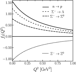
Figure 1: SHD form factors $f_{1}^{B_{1}B_{2}}(Q^{2})$ and $f_{2}^{B_{1}B_{2}}(Q^{2})$ in the self-consitent $\chi$QSM for $M=420$ MeV with linear $m_{s}$ corrections taken into account. In the upper panel, the form factors for the $\Delta S=0$ transitions are drawn and in the lower panel those for the $\Delta s=1$ transitions are depicted.

It is also of great interest to compare the present results with the recent investigation of $f_{2}^{B_{1}B_{2}}(0)$ and $\langle r_{f_{1}}\rangle^{2}$ for the $\Delta S=1$ transitions in $\chi$PT to order $\mathcal{O}(p^{4})$ [52]. As shown in Table 5, they are in good agreement each other except for the $\Xi^{-}\to\Sigma^{0}$ transition.

Table 5: Comparison of the final results of $\chi\textrm{QSM}_{m_{s}^{0}+m_{s}^{1}}$ for $\langle r_{f_{1}}\rangle^{2}$ and $f_{2}(0)$ with those of $\chi$PT to order $\mathcal{O}(p^{4})$ [52] in which the normalization is given as $f_{2}(0)=\kappa\frac{m_{1}}{2m_{p}}$.

$\langle r_{f_{1}}\rangle^{2}/\textrm{fm}^{2}$	$\chi$PT $\mathcal{O}(p^{4})$	$\chi$QSM
$\Sigma^{-}\to n$	$0.72$	$0.60$
$\Lambda\to p$	$0.70$	$0.72$
$\Xi^{-}\to\Sigma^{0}$	$0.77$	$0.80$
$\Xi^{-}\to\Lambda$	$0.65$	$0.66$

$f_{2}^{B_{1}B_{2}}(0)$	$\chi$PT $\mathcal{O}(p^{4})$	$\chi$QSM
$\Sigma^{-}\to n$	$-1.00$	$-0.96$
$\Lambda\to p$	$0.88$	$0.88$
$\Xi^{-}\to\Sigma^{0}$	$1.90$	$1.43$
$\Xi^{-}\to\Lambda$	$-0.05$	$-0.03$

4.2 SHD axial-vector form factors

We present now the results of the SHD axial-vector form factors $g_{1}^{B_{1}B_{2}}(Q^{2})$. The SHD axial-vector constants are insensitive to the constituent quark mass $M$. Varying $M$ from $400$ to $450$ MeV, they are changed just by about $5\,\%$. The linear $m_{s}$ corrections turn out to be also small. Figure 2 depicts the SHD axial-vector form factors $g_{1}^{B_{1}B_{2}}(Q^{2})$ for all relevant processes. The dipole parameterization is used for fitting the axial-vector form factors in the $\chi$QSM:

$$g_{1}^{B_{1}B_{2}}(Q^{2})=\frac{g_{1}^{B_{1}B_{2}}(0)}{(1+Q^{2}/M_{g_{1}}^{2})^{2}},$$ (72)

where the corresponding radius is again given as $\langle r_{g_{1}}\rangle^{2}=12/M_{g_{1}}^{2}$. The axial-vector constants and dipole masses are given in Table 6. In flavor $SU(3)$ symmetry, the axial-vector part of the SHD can be characterized by two form factors $F(Q^{2})$ and $D(Q^{2})$ that are related to the proton triplet and octet axial-vector form factors:

$$g_{A}^{3}(Q^{2}) = F(Q^{2})+D(Q^{2}),$$ (73)

$$g_{A}^{8}(Q^{2}) = \frac{1}{\sqrt{3}}\Big{(}3F(Q^{2})-D(Q^{2})\Big{)}.$$ (74)

The triplet and octet axial-vector constants $g_{A}^{3}(0)$ and $g_{A}^{8}(0)$ have been already calculated explicitly in the $\chi$QSM [29] by using exactly the present formalism. The corresponding values of $F$ and $D$ are given below, where linear $m_{s}$ corrections are taken into account:

$$g_{A}^{3}(0)=1.16, F(0)=0.446,\;\;\;\;\;F(0)^{exp}=0.462\pm 0.008,$$ (75)

$$g_{A}^{8}(0)=0.36, D(0)=0.714,\;\;\;\;\;D(0)^{exp}=0.804\pm 0.008.$$ (76)

In Table 7, the final results of the ratios $(g_{1}(0)/f_{1}(0))^{B_{1}B_{2}}$ are listed with and without linear $m_{s}$-corrections considered and are compared with the experimental data. Note that these ratios were also investigated in the $\chi$QSM without the symmetry-conserving quantization [8] and in the infinite momentum frame [48] in flavor $SU(3)$ symmetry. T he flavor $SU(3)$-symmetry breaking contributions are negligible and the effect of the symmetry-conserving quantization is moderate.

Table 6: Results of the SHD axial-vector $g_{1}^{B_{1}B_{2}}(0)$ constants and dipole masses $M_{g_{1}}^{B_{1}B_{2}}$ in the self-consistent $\chi$QSM for $M=420$ MeV. The first two columns show the results without and with $m_{s}$ corrections, respectively. The third column shows those calculated in $SU(3)$ symmetry by using the results of the proton $g_{A}^{3}$ and $g_{A}^{8}$ constants in the $\chi$QSM. The dipole masses are given in units of GeV with linear $m_{s}$ corrections taken into account.

$g_{1}(0)$	$\chi\textrm{QSM}_{\mathrm{SU(3)}}$	$\chi\textrm{QSM}_{m_{s}^{0}+m_{s}^{1}}$	$\chi\textrm{QSM}_{\mathrm{SU(3)}}$	$M_{g_{1}}/$GeV
$n\to p$	$1.16$	$1.18$	$F+D=1.16$	$1.04$
$\Sigma^{-}\to\Lambda$	$0.58$	$0.60$	$\sqrt{\frac{2}{3}}D=0.58$	$1.04$
$\Sigma^{-}\to\Sigma^{0}$	$0.63$	$0.65$	$\sqrt{2}F=0.63$	$1.04$
$\Xi^{-}\to\Xi^{0}$	$-0.27$	$-0.27$	$F-D=-0.27$	$1.05$
$\Sigma^{-}\to n$	$-0.27$	$-0.27$	$F-D=-0.27$	$1.05$
$\Lambda\to p$	$0.83$	$0.83$	$\sqrt{\frac{3}{2}}(F+D/3)=0.84$	$1.06$
$\Xi^{-}\to\Sigma^{0}$	$0.82$	$0.82$	$\sqrt{\frac{1}{2}}(F+D)=0.82$	$1.06$
$\Xi^{-}\to\Lambda$	$0.25$	$0.26$	$\sqrt{\frac{3}{2}}(F-D/3)=0.25$	$1.05$

Figure 2: SHD axial-vector form factors $g^{B_{1}B_{2}}_{1}(Q^{2})$ in the self-consistent $\chi$QSM for $M=420$ MeV with linear $m_{s}$ corrections taken into account. In the left and right panels, the form factors for the $\Delta S=0$ and $\Delta S=1$ transitions are drawn, respectively.

Table 7: Results for the ratios $(g_{1}/f_{1})$. The first two columns show the results of this work with and without $m_{s}$ corrections, where our final results are given by $\chi\textrm{QSM}_{m_{s}^{0}+m_{s}^{1}}$. The other two columns correspond to those of the $\chi$QSM in the Fock representation on the light cone [48] and to those of the old $\chi$QSM [8] without symmetry conserving quantization, respectively. Experimental data are taken from Ref. [46, 13, 12]. For the $\Sigma^{-}\to\Lambda$ decay the value of $\sqrt{\frac{3}{2}}\cdot g_{1}^{\Sigma\Lambda}(0)$ is listed.

$g_{1}/f_{1}$	$\chi\textrm{QSM}_{\mathrm{SU(3)}}$	$\chi\textrm{QSM}_{m_{s}^{0}+m_{s}^{1}}$	IMF [48]	’98 [8]	Exp.
$n\to p$	$1.16$	$1.18$	$1.156$	$1.42$	$1.2695\pm 0.0029$
$\Sigma^{-}\to\Lambda$	$0.71$	$0.73$	$0.686$	$0.91$	$0.720\pm 0.020$
$\Sigma^{-}\to\Sigma^{0}$	$0.45$	$0.46$	$0.470$	$0.55$
$\Xi^{-}\to\Xi^{0}$	$-0.27$	$-0.27$	$-0.215$
$\Sigma^{-}\to n$	$-0.27$	$-0.27$	$-0.215$	$-0.31$	$-0.340\pm 0.017$
$\Lambda\to p$	$0.68$	$0.68$	$0.699$	$0.73$	$0.718\pm 0.015$
$\Xi^{-}\to\Sigma^{0}$	$1.16$	$1.16$	$1.156$	$1.29$	$1.25_{-0.16}^{+0.14}$
$\Xi^{-}\to\Lambda$	$0.20$	$0.21$	$0.242$	$0.22$	$0.25\pm 0.05$

It is also interesting to consider the ratio of $\Lambda\to pe^{-}\overline{\nu}$ to $\Sigma^{-}\to ne^{-}\overline{\nu}$, since it is known experimentally. The comparison can be found in the following:

$$\frac{(g_{1}/f_{1})[\Lambda\to pe^{-}\overline{\nu}]}{(g_{1}/f_{1})[\Sigma^{-}\to ne^{-}\overline{\nu}]}=-2.52,\;\;\;\;\textrm{Exp.:}-2.11\pm 0.15.$$ (77)

The result is in qualitative agreement with the data.

In flavor $SU(3)$ symmetry, the transitions $\Xi^{0}\to\Sigma^{+}e^{-}\bar{\nu}_{e}$ and $n\to pe^{-}\bar{\nu}_{e}$ are identical except that the valence d quarks are replaced by s quarks in the initial and final state baryons, respectively. In this case, only the CKM matrix elements become important to distinguish these decay amplitudes. Experimental values for the $\Xi^{0}\to\Sigma^{+}e^{-}\bar{\nu}_{e}$ decay are available from Ref. [10] and recently also from Ref.[11]. The extracted value of $g_{1}/f_{1}$ for $\Xi^{0}\to\Sigma^{+}e^{-}\overline{\nu_{e}}$ is presented as

$$\Big{(}g_{1}/f_{1}\Big{)}^{\Xi^{0}\Sigma^{+}}_{\textrm{KTeV}}=1.32_{-0.17\textrm{stat}}^{+0.21}\pm 0.05_{\textrm{syst}},\;\;\;\;\Big{(}g_{1}/f_{1}\Big{)}^{\Xi^{0}\Sigma^{+}}_{\textrm{NA48/I}}=1.20\pm 0.05.$$ (78)

In the present work with $SU(3)$-symmetry breaking, we obtain the following result:

$$\Big{(}g_{1}/f_{1}\Big{)}^{\Xi^{0}\Sigma^{+}}_{\chi\textrm{QSM}}=\Big{(}\sqrt{2}\cdot g_{1}/(\sqrt{2}\cdot f_{1})\Big{)}^{\Xi^{-}\Sigma^{0}}_{\chi\textrm{QSM}}=\Big{(}\sqrt{2}\cdot g_{1}/1\Big{)}^{\Xi^{-}\Sigma^{0}}_{\chi\textrm{QSM}}=1.16,$$ (79)

which is close to the above experimental data as well as to the values of $g_{1}/f_{1}$ for $n\to pe^{-}\bar{\nu}_{e}$

$$\Big{(}g_{1}/f_{1}\Big{)}^{np}_{\textrm{exp.}}=1.2695\pm 0.0029,\,\,\,\,\,\,\,\,\,\,\,\,\,\,\ \Big{(}g_{1}/f_{1}\Big{)}^{np}_{\chi\textrm{QSM}}=1.18,$$ (80)

showing explicitly that $m_{s}$ contributions to the SHD are small.

In Ref. [20], the CKM matrix element $V_{us}$ was extracted within a large $N_{c}$ approach. The SHD form factors $f_{1}$, $f_{2}$ and $g_{1}$ were fitted to experimental decay rates, angular correlation, and asymmetry coefficients. The present work is consistent with the values presented in Ref. [20]. Very recently, a lattice study of the $\Sigma^{-}\to nl\nu$ decay was performed [53]. A polynomial extrapolation to the physical point yields the value of $g_{1}(0)/f_{1}(0)=-0.287\pm 0.052$ with $g_{2}(0)=0$. The corresponding result of the present work in Table 7 is $g_{1}(0)/f_{1}(0)=-0.27$, which is consistent with the lattice one. The authors of Ref. [53] also computed $g_{2}(0)$ and obtained a rather large value of $g_{2}(0)/f_{1}(0)=+0.63\pm 0.26$. They calculated $|(g_{1}-0.133g_{2})/f_{1}|=0.37\pm 0.08$ which is in good agreement with the experimental value of $|(g_{1}-0.133g_{2})/f_{1}|=0.327\pm 0.007_{\textrm{stat}}\pm 0.019_{\textrm{syst}}$ extracted in Ref. [51]. The $g_{2}(Q^{2})$ could also be calculated in the $\chi$QSM and in this way one could check if also there a scenario with a large $g_{2}(0)$ comes out. In Ref. [22], the SHD were investigated in a relativistic quark model, the results of the present work are compatible with those of Ref. [22]. The dipole mass was extracted in Refs. [6, 54]: $M_{A}=1.08\pm 0.08$ GeV for the $n\to p$ decay and $M_{A}=1.25$ GeV for $\Delta S=1$ decays. References [55, 56] presented $M_{A}=0.96$ GeV for the $\Delta S=0$ decays and $M_{A}=1.11$ GeV for $\Delta S=1$. The corresponding results of the present work are given as $M_{A}\approx 1.04$ GeV and $M_{A}=1.06$ GeV.

5 Summary and Conclusion

In the present work we investigated the semileptonic hyperon decays (SHD) within the framework of the self-consistent SU(3) chiral quark-soliton model. We take into account the linear rotational $1/N_{c}$ corrections as well as linear $m_{s}$ corrections and employ the symmetry-conserving quantization. In particular, we calculated the SHD vector form factors $f_{1}(Q^{2})$ and $f_{2}(Q^{2})$ and axial-vector form factors $g_{1}(Q^{2})$ for all relevant decays in the baryon octet. Since $f_{3}(Q^{2})$ and $g_{3}(Q^{2})$ are always multiplied by a factor of $(m_{e}/M_{B})^{2}$ in the transition amplitudes, we neglected them. The form factor $g_{2}(Q^{2})$ was neglected, assuming that it is very small.

The chiral quark-soliton model has been applied for many years successfully to various obseervables in the hadronic and partonic sector. All numerical parameters of the present investigation are the same as in previous works and were fixed by only four basic pion and nucleon observables. A self-consistent soliton profile is used in order to solve numerically for eigenvalues of the $\chi$QSM single-particle Hamiltonian. These eigenvalues were then used for calculating every form factor of the present work.

We first discussed the results for the SHD constants at $Q^{2}=0$ of the form factors $f_{1}$ and $f_{2}$, see Table 2 for the final results. Since we only consider the linear $m_{s}$-corrections, we have the flavor-$SU(3)$ symmetric results for $f_{1}(0)$, which is a consequence of the Ademollo-Gatto theorem. Our values of $f_{2}/f_{1}$ agree qualitatively with those of the Cabibbo model without and with $SU(3)$-symmetry breaking as well as with experimental data, see Table 3 for the final results. Especially, the SHD constants for the $\Sigma^{-}\to n$ and $\Xi^{0}\to\Sigma^{+}$ processes agree very well with the new experimental data. The $m_{s}$ corrections to $f_{2}(0)$ for both the $\Delta S=0$ and $\Delta S=1$ transitions turn out to be sizeable in accrodance with previous calculations in the $\chi$QSM. The vector radii and dipole masses were listed in Table 4. The dipole mass for the $n\to p$ decay was obtained as $M^{np}_{f_{1}}=0.752$ GeV which is comparable to those in the literature. The $\Delta S=1$ constants $f_{2}(0)$ and radii of $f_{1}(Q^{2})$ in the $\chi$QSM do also agree with a calculation in chiral perturbation theory to order $\mathcal{O}(p^{4})$.

Second, we discussed the SHD constants and dipole masses of the axial-vector form factor $g_{1}(Q^{2})$, see Tables 6 and 7 for the final results. The dipole masses for the $\Delta S=0$ decays turned out to be $M_{g_{1}}=1.04$ GeV and for the $\Delta S=1$ decays $M_{g_{1}}=1.06$ GeV. The results of the SHD axial-vector constants of the present work are in good agreement with calculations done in the Fock state representation of the $\chi$QSM on the light cone. Various $m_{s}$ corrections in the form factor $g_{1}(Q^{2})$ destructively interfere, so that the total $m_{s}$ corrections become rather small. The application of the symmetry-conserving quantization reduces the $m_{s}$ corrections even further. The first determination of $(g_{1}/f_{1})$ for the process $\Sigma^{-}\to nl\nu$ on the lattice yielded a value of $-0.287\pm 0.052$, while the present work gives $-0.27$. In addition, the chiral quark-soliton model reproduces very well the recent measured value of $(g_{1}/f_{1})=1.20\pm 0.05$ by the NA48/I collaboration. Overall, the chiral quark-soliton model with the present techniques reproduces the existing experimental data very accurately. Since the chiral quark-soliton model is the simplest current quark model showing spontaneous breaking of chiral symmetry the present calculation shows how important this effect is for the physics of light baryons.

Appendix A Form Factors in the $\chi$QSM

The electric density in Eq.(45) is given by

$$\mathcal{G}_{E}^{\chi}({\bm{z}}) = D_{\chi 8}^{(8)}\sqrt{\frac{1}{3}}\mathcal{B}({\bm{z}})-\frac{2}{I_{1}}D_{\chi i}^{(8)}J_{i}\mathcal{I}_{1}({\bm{z}})-\frac{2}{I_{2}}D_{\chi a}^{(8)}J_{a}\mathcal{I}_{2}({\bm{z}})$$ (81)

$$-\frac{2}{\sqrt{3}}M_{1}D_{\chi 8}^{(8)}\mathcal{C}({\bm{z}})-\frac{2}{3}M_{8}D_{88}^{(8)}D_{\chi 8}^{(8)}\mathcal{C}({\bm{z}})$$

$$+4\frac{K_{1}}{I_{1}}M_{8}D_{8i}^{(8)}D_{\chi i}^{(8)}({\bm{z}})\mathcal{I}_{1}({\bm{z}})+4\frac{K_{2}}{I_{2}}M_{8}D_{8a}^{(8)}D_{\chi a}^{(8)}\mathcal{I}_{2}({\bm{z}})$$

$$-4M_{8}D_{8i}^{(8)}D_{\chi i}^{(8)}\mathcal{K}_{1}({\bm{z}})-4M_{8}D_{\chi a}^{(8)}D_{8a}^{(8)}\mathcal{K}_{2}({\bm{z}}),$$

and the magnetic density in Eq.(46) by

$$\mathcal{G}_{M}^{\chi}({\bm{z}}) = -\sqrt{3}D_{\chi 3}^{(8)}\mathcal{Q}_{0}({\bm{z}})-\frac{1}{\sqrt{3}}\frac{1}{I_{1}}D_{\chi 8}^{(8)}J_{3}\mathcal{X}_{1}({\bm{z}})+\sqrt{3}\frac{1}{I_{1}}d_{ab3}D_{\chi b}^{(8)}J_{a}\mathcal{X}_{2}({\bm{z}})+\sqrt{\frac{1}{2}}\frac{1}{I_{1}}D_{\chi 3}^{(8)}\mathcal{Q}_{1}({\bm{z}})$$ (82)

$$+\frac{2}{\sqrt{3}}\frac{K_{1}}{I_{1}}M_{8}D_{83}^{(8)}D_{\chi 8}^{(8)}\mathcal{X}_{1}({\bm{z}})-2\sqrt{3}\frac{K_{2}}{I_{2}}M_{8}D_{8a}^{(8)}D_{\chi b}^{(8)}d_{ab3}\mathcal{X}_{2}({\bm{z}})$$

$$+2\sqrt{3}\Big{[}M_{1}D_{\chi 3}^{(8)}+\frac{1}{\sqrt{3}}M_{8}D_{88}^{(8)}D_{\chi 3}^{(8)}\Big{]}\mathcal{M}_{0}({\bm{z}})$$

$$-\frac{2}{\sqrt{3}}M_{8}D_{83}^{(8)}D_{\chi 8}^{(8)}\mathcal{M}_{1}({\bm{z}})+2\sqrt{3}M_{8}D_{\chi a}^{(8)}D_{8b}^{(8)}d_{ab3}\mathcal{M}_{2}({\bm{z}}).$$

The axial-vector density in Eq.(47) is given by

$$\mathcal{G}_{10}^{\chi}({\bm{z}}) = -\sqrt{\frac{1}{3}}D_{\chi 3}^{(8)}\mathcal{A}({\bm{z}})+\frac{1}{3\sqrt{3}}\frac{1}{I_{1}}D_{\chi 8}^{(8)}J_{3}\mathcal{B}({\bm{z}})-\sqrt{\frac{1}{3}}\frac{1}{I_{2}}D_{\chi a}^{(8)}J_{b}d^{ab3}\mathcal{C}({\bm{z}})$$ (83)

$$-\frac{1}{3\sqrt{2}}\frac{1}{I_{1}}D_{\chi 3}^{(8)}\mathcal{D}({\bm{z}})-\frac{2}{3\sqrt{3}}\frac{K_{1}}{I_{1}}M_{8}D_{83}^{(8)}D_{\chi 8}^{(8)}\mathcal{B}({\bm{z}})+\frac{2}{\sqrt{3}}\frac{K_{2}}{I_{2}}\,M_{8}\,D_{8a}^{(8)}D_{\chi b}^{(8)}d^{ab3}\mathcal{C}({\bm{z}})$$

$$-\frac{2}{\sqrt{3}}\Big{[}M_{1}D_{\chi 3}^{(8)}+\frac{1}{\sqrt{3}}M_{8}D_{88}^{(8)}D_{\chi 3}^{(8)}\Big{]}\mathcal{H}({\bm{z}})$$

$$+\frac{2}{3\sqrt{3}}M_{8}D_{83}^{(8)}D_{\chi 8}^{(8)}\mathcal{I}({\bm{z}})-\frac{2}{\sqrt{3}}M_{8}D_{8a}^{(8)}D_{\chi b}^{(8)}d^{ab3}\mathcal{J}({\bm{z}}).$$

The explicit expressions for $\mathcal{B}({\bm{z}}),\mathcal{I}_{1}({\bm{z}}),\cdots,\mathcal{J}({\bm{z}})$ can be found in the following Appendices for each form factor. The baryon matrix-elements, such as $\langle B^{\prime}|D_{\chi 3}^{(8)}|B\rangle$, are evaluated by using the $SU(3)$ group algebra [58, 57]

$$\langle B_{\mathcal{R}^{\prime}}^{\prime}|D_{\chi m}^{n}(A)|B_{\mathcal{R}}\rangle = \sqrt{\frac{\textrm{dim}\mathcal{R}^{\prime}}{\textrm{dim}\mathcal{R}}}(-1)^{\frac{1}{2}Y_{s}^{\prime}+S_{3}^{\prime}}(-1)^{\frac{1}{2}Y_{s}+S_{3}}$$ (88)

$$\times\sum_{\gamma}\left(\begin{array}[]{ccc}\mathcal{R}^{\prime}&n&\mathcal{R}_{\gamma}\\ Q^{\prime}&\chi&Q\end{array}\right)\left(\begin{array}[]{ccc}\mathcal{R}^{\prime}&n&\mathcal{R}_{\gamma}\\ -Y_{s}^{\prime}S^{\prime}-S_{3}^{\prime}&m&-Y_{S}S-S_{3}\end{array}\right)\,\,\,,$$

with $Q=YII_{3}$. $\left(\cdots\right)$ denote the $SU(3)$ Clebsch-Gordan coefficients. The results for all transitions in Eqs.(2,3) are listed below.

Appendix B Form Factor Densities

B.1 $\chi$QSM Electric Densities

The electric densities are

$$\frac{1}{N_{c}}\mathcal{B}({\bm{z}}) = \varphi_{v}^{\dagger}({\bm{z}})\varphi_{v}({\bm{z}})-\frac{1}{2}\sum_{n}\textrm{sign}(\varepsilon_{n})\phi_{n}^{\dagger}({\bm{z}})\phi_{n}({\bm{z}}),$$

$$\frac{\delta^{ij}}{N_{c}}\mathcal{I}_{1}({\bm{z}}) = \frac{1}{2}\sum_{\varepsilon_{n}\neq\varepsilon_{v}}\frac{1}{\varepsilon_{n}-\varepsilon_{v}}\langle v|\tau^{i}|n\rangle\phi_{n}^{\dagger}({\bm{z}})\tau^{j}\phi_{v}({\bm{z}})+\frac{1}{4}\sum_{n,m}\mathcal{R}_{3}(\varepsilon_{n},\varepsilon_{m})\langle n|\tau^{i}|m\rangle\phi_{m}^{\dagger}({\bm{z}})\tau^{j}\phi_{n}({\bm{z}}),$$

$$\frac{1}{N_{c}}\mathcal{I}_{2}({\bm{z}}) = \frac{1}{4}\sum_{\varepsilon_{n^{0}}}\frac{1}{\varepsilon_{n^{0}}-\varepsilon_{v}}\langle n^{0}|v\rangle\phi_{v}^{\dagger}({\bm{z}})\phi_{n^{0}}({\bm{z}})+\frac{1}{4}\sum_{n,m^{0}}\mathcal{R}_{3}(\varepsilon_{n},\varepsilon_{m^{0}})\phi_{m^{0}}^{\dagger}({\bm{z}})\phi_{n}({\bm{z}})\langle n|m^{0}\rangle,$$

$$\frac{1}{N_{c}}\mathcal{C}({\bm{z}}) = \sum_{\varepsilon_{n}\neq\varepsilon_{v}}\frac{1}{\varepsilon_{n}-\varepsilon_{v}}\phi_{v}^{\dagger}({\bm{z}})\phi_{n}({\bm{z}})\langle n|\gamma^{0}|v\rangle+\frac{1}{2}\sum_{n,m}\langle n|\gamma^{0}|m\rangle\phi_{m}^{\dagger}({\bm{z}})\phi_{n}({\bm{z}})\mathcal{R}_{5}(\varepsilon_{n},\varepsilon_{m}),$$

$$\frac{\delta^{ij}}{N_{c}}\mathcal{K}_{1}({\bm{z}}) = \frac{1}{2}\sum_{\varepsilon_{n}\neq\varepsilon_{v}}\frac{1}{\varepsilon_{n}-\varepsilon_{v}}\langle v|\gamma^{0}\tau^{i}|n\rangle\phi_{n}^{\dagger}({\bm{z}})\tau^{j}\phi_{v}({\bm{z}})+\frac{1}{4}\sum_{n,m}\langle n|\gamma^{0}\tau^{i}|m\rangle\phi_{m}^{\dagger}({\bm{z}})\tau^{j}\phi_{n}({\bm{z}})\mathcal{R}_{5}(\varepsilon_{n},\varepsilon_{m}),$$

$$\frac{1}{N_{c}}\mathcal{K}_{2}({\bm{z}}) = \frac{1}{4}\sum_{\varepsilon_{n^{0}}}\frac{1}{\varepsilon_{n^{0}}-\varepsilon_{v}}\phi_{v}^{\dagger}({\bm{z}})\phi_{n^{0}}({\bm{z}})\langle n^{0}|\gamma^{0}|v\rangle+\frac{1}{4}\sum_{n,m}\mathcal{R}_{5}(\varepsilon_{n},\varepsilon_{m^{0}})\phi_{m^{0}}^{\dagger}({\bm{z}})\phi_{n}({\bm{z}})\langle n|\gamma^{0}|m^{0}\rangle.$$

The vectors $\langle n|$ are eigenstates of the $\chi$QSM Hamiltonian $H(U)$ which are a linear combination of the eigenstates $\langle n^{0}|$ of the Hamiltonian $H(1)$ [59].

B.2 $\chi$QSM Magnetic Densities

The operator for the magnetic form factors in the $\chi$QSM is $O_{1}=\gamma^{0}[{\bm{z}}\times{\bm{\gamma}}]_{3}=\gamma^{5}[{\bm{z}}\times{\bm{\sigma}}]_{10}$ and the magnetic densities are

$$\frac{1}{N_{c}}\mathcal{Q}_{0}({\bm{z}}) = \langle v||{\bm{z}}\rangle\{O_{1}\otimes\tau_{1}\}_{0}\langle{\bm{z}}||v\rangle+\sum_{n}\sqrt{2G_{n}+1}\langle n||{\bm{z}}\rangle\{O_{1}\otimes\tau_{1}\}_{0}\langle{\bm{z}}||n\rangle\mathcal{R}_{1}(\varepsilon_{n}),$$

$$\frac{1}{N_{c}}\mathcal{X}_{1}({\bm{z}}) = \sum_{\varepsilon_{n}\neq\varepsilon_{v}}\frac{1}{\varepsilon_{n}-\varepsilon_{v}}(-)^{G_{n}}\langle v||{\bm{z}}\rangle O_{1}\langle{\bm{z}}||n\rangle\langle n||\tau_{1}||v\rangle$$

$$+\frac{1}{2}\sum_{n,m}\mathcal{R}_{5}(\varepsilon_{n},\varepsilon_{m})(-)^{G_{m}-G_{n}}\langle n||\tau_{1}||m\rangle\langle m||{\bm{z}}\rangle O_{1}\langle{\bm{z}}||n\rangle,$$

$$\frac{1}{N_{c}}\mathcal{X}_{2}({\bm{z}}) = \sum_{\varepsilon_{n^{0}}}\frac{1}{\varepsilon_{n^{0}}-\varepsilon_{v}}\langle n^{0}||{\bm{z}}\rangle\{O_{1}\otimes\tau_{1}\}_{0}\langle{\bm{z}}||v\rangle\langle v\mid n^{0}\rangle$$

$$+\sum_{n,m^{0}}\mathcal{R}_{5}(\varepsilon_{n},\varepsilon_{m^{0}})\sqrt{2G_{m}+1}\langle m^{0}||{\bm{z}}\rangle\{O_{1}\otimes\tau_{1}\}_{0}\langle{\bm{z}}||n\rangle\langle n\mid m^{0}\rangle,$$

$$\frac{1}{N_{c}}\mathcal{Q}_{1}({\bm{z}}) = \sum_{\varepsilon_{n}}\frac{\textrm{sign}(\varepsilon_{n})}{\varepsilon_{n}-\varepsilon_{v}}(-)^{G_{n}}\langle n||{\bm{z}}\rangle\{O_{1}\otimes\tau_{1}\}_{1}\langle{\bm{z}}||v\rangle\langle v||\tau_{1}||n\rangle$$

$$+\frac{1}{2}\sum_{n,m}\mathcal{R}_{4}(\varepsilon_{n},\varepsilon_{m})(-)^{G_{m}-G_{n}}\langle n||{\bm{z}}\rangle\{O_{1}\otimes\tau_{1}\}_{1}\langle{\bm{z}}||m\rangle\langle m||\tau_{1}||n\rangle,$$

$$\frac{1}{N_{c}}\mathcal{M}_{0}({\bm{z}}) = \sum_{\varepsilon_{n}\neq\varepsilon_{v}}\frac{1}{\varepsilon_{n}-\varepsilon_{v}}\langle v||{\bm{z}}\rangle\{O_{1}\otimes\tau_{1}\}_{0}\langle{\bm{z}}||n\rangle\langle n|\gamma^{0}|v\rangle$$

$$-\frac{1}{2}\sum_{n,m}\mathcal{R}_{2}(\varepsilon_{n},\varepsilon_{m})\sqrt{2G_{m}+1}\langle n|\gamma^{0}|m\rangle\langle m||{\bm{z}}\rangle\{O_{1}\otimes\tau_{1}\}_{0}\langle{\bm{z}}||n\rangle,$$

$$\frac{1}{N_{c}}\mathcal{M}_{1}({\bm{z}}) = \sum_{\varepsilon_{n}\neq\varepsilon_{v}}\frac{1}{\varepsilon_{n}-\varepsilon_{v}}(-)^{G_{n}}\langle n||\gamma^{0}\tau_{1}||v\rangle\langle v||{\bm{z}}\rangle O_{1}\langle{\bm{z}}||n\rangle$$

$$-\frac{1}{2}\sum_{n,m}\mathcal{R}_{2}(\varepsilon_{n},\varepsilon_{m})(-)^{G_{m}-G_{n}}\langle n||\gamma^{0}\tau_{1}||m\rangle\langle m||{\bm{z}}\rangle O_{1}\langle{\bm{z}}||n\rangle,$$

$$\frac{1}{N_{c}}\mathcal{M}_{2}({\bm{z}}) = \sum_{\varepsilon_{n^{0}}}\frac{1}{\varepsilon_{n^{0}}-\varepsilon_{v}}\langle v||{\bm{z}}\rangle\{O_{1}\otimes\tau_{1}\}_{0}\langle{\bm{z}}||n^{0}\rangle\langle n^{0}|\gamma^{0}|v\rangle$$

$$-\sum_{n,m^{0}}\mathcal{R}_{2}(\varepsilon_{n},\varepsilon_{m^{0}})\sqrt{2G_{m}+1}\langle m^{0}||{\bm{z}}\rangle\{O_{1}\otimes\tau_{1}\}_{0}\langle{\bm{z}}||n\rangle\langle n|\gamma^{0}|m^{0}\rangle.$$

B.3 $\chi$QSM Axial-vector Densities

Two parts in Eq.(47) correspond to the density Eq.(83) with the expressions $\mathcal{A}({\bm{z}}),\mathcal{B}({\bm{z}})...$ once calculated with the operator

$$O_{1}=\gamma^{0}\gamma_{3}\gamma^{5}\,\,\,\,\,\,\,\,\,\,\,\,\,\,\,\textrm{and once with}\,\,\,\,\,\,\,\,\,\,\,\,\,\,\,O_{1}=\gamma^{0}\{Y_{2}\otimes\gamma_{1}\}_{10}\gamma^{5}=1\cdot\{Y_{2}\otimes\gamma_{1}\}_{10}\,\,\,,$$ (89)

yielding once $\mathcal{G}_{10}^{\chi}({\bm{z}})$ and $\{Y_{2}\otimes\mathcal{G}_{1}^{\chi}({\bm{z}})\}_{10}$ in the tensor-notation of [60], respectively. We have for $\mathcal{A}({\bm{z}}),\mathcal{B}({\bm{z}})...$:

$$\frac{1}{N_{c}}\mathcal{A}({\bm{z}}) = \langle v||{\bm{z}}\rangle\{O_{1}\otimes\tau_{1}\}_{0}\langle{\bm{z}}||v\rangle+\sum_{n}\sqrt{2G+1}\mathcal{R}_{1}(\varepsilon_{n})\langle n||{\bm{z}}\rangle\{O_{1}\otimes\tau_{1}\}_{0}\langle{\bm{z}}||n\rangle,$$

$$\frac{1}{N_{c}}\mathcal{B}({\bm{z}}) = \sum_{\varepsilon_{n}\neq\varepsilon_{v}}\frac{1}{\varepsilon_{v}-\varepsilon_{n}}(-)^{G_{n}}\langle n||{\bm{z}}\rangle O_{1}\langle{\bm{z}}||v\rangle\langle v||\tau_{1}||n\rangle$$

$$-\frac{1}{2}\sum_{n,m}(-)^{G_{n}-G_{m}}\langle m||{\bm{z}}\rangle O_{1}\langle{\bm{z}}||n\rangle\langle n||\tau_{1}||m\rangle\mathcal{R}_{5}(\varepsilon_{n},\varepsilon_{m}),$$

$$\frac{1}{N_{c}}\mathcal{C}({\bm{z}}) = \sum_{\varepsilon_{n^{0}}}\frac{1}{\varepsilon_{v}-\varepsilon_{n^{0}}}\langle v||{\bm{z}}\rangle\{O_{1}\otimes\tau_{1}\}_{0}\langle{\bm{z}}||n^{0}\rangle\langle n^{0}|v\rangle$$

$$-\sum_{n,m}\sqrt{2G_{n}+1}\langle n||{\bm{z}}\rangle\{O_{1}\otimes\tau_{1}\}_{0}\langle{\bm{z}}||m^{0}\rangle\langle m^{0}|n\rangle\mathcal{R}_{5}(\varepsilon_{n},\varepsilon_{m^{0}}),$$

$$\frac{1}{N_{c}}\mathcal{D}({\bm{z}}) = \sum_{n}\frac{\textrm{sign}(\varepsilon_{n})}{\varepsilon_{v}-\varepsilon_{n}}(-)^{G_{n}}\langle n||{\bm{z}}\rangle\{O_{1}\otimes\tau_{1}\}_{1}\langle{\bm{z}}||v\rangle\langle v||\tau_{1}||n\rangle$$

$$+\frac{1}{2}\,\sum_{n,m}\mathcal{R}_{4}(\varepsilon_{n},\varepsilon_{m})(-)^{G_{n}-G_{m}}\langle m||{\bm{z}}\rangle\{O_{1}\otimes\tau_{1}\}_{1}\langle{\bm{z}}||n\rangle\langle n||\tau_{1}||m\rangle,$$

$$\frac{1}{N_{c}}\mathcal{H}({\bm{z}}) = \sum_{\varepsilon_{n}\neq\varepsilon_{v}}\,\frac{1}{\varepsilon_{v}-\varepsilon_{n}}\langle v||{\bm{z}}\rangle\{O_{1}\otimes\tau_{1}\}_{0}\langle{\bm{z}}||n\rangle\langle n|\gamma^{0}|v\rangle$$

$$+\frac{1}{2}\sum_{n,m}\mathcal{R}_{2}(\varepsilon_{n},\varepsilon_{m})\sqrt{2G_{m}+1}\langle m||{\bm{z}}\rangle\{O_{1}\otimes\tau_{1}\}_{0}\langle{\bm{z}}||n\rangle\langle n|\gamma^{0}|m\rangle,$$

$$\frac{1}{N_{c}}\mathcal{I}({\bm{z}}) = \sum_{\varepsilon_{n}\neq\varepsilon_{v}}\,\frac{1}{\varepsilon_{v}-\varepsilon_{n}}(-)^{G_{n}}\langle v||{\bm{z}}\rangle O_{1}\langle{\bm{z}}||n\rangle\langle n||\gamma^{0}\tau_{1}||v\rangle$$

$$+\frac{1}{2}\sum_{n,m}\mathcal{R}_{2}(\varepsilon_{n},\varepsilon_{m})(-)^{G_{n}-G_{m}}\langle m||{\bm{z}}\rangle O_{1}\langle{\bm{z}}||n\rangle\langle n||\gamma^{0}\tau_{1}||m\rangle,$$

$$\frac{1}{N_{c}}\mathcal{J}({\bm{z}}) = \sum_{\varepsilon_{n^{0}}}\,\frac{1}{\varepsilon_{v}-\varepsilon_{n^{0}}}\langle v||{\bm{z}}\rangle\{O_{1}\otimes\tau_{1}\}_{0}\langle{\bm{z}}||n^{0}\rangle\langle n^{0}|\gamma^{0}|v\rangle$$

$$+\sum_{n,m}\mathcal{R}_{2}(\varepsilon_{n^{0}},\varepsilon_{m})\sqrt{2G_{m}+1}\langle m||{\bm{z}}\rangle\{O_{1}\otimes\tau_{1}\}_{0}\langle{\bm{z}}||n^{0}\rangle\langle n^{0}|\gamma^{0}|m\rangle.$$

B.4 Regularization Functions

The regularization functions are defined as:

$$\mathcal{R}_{1}(\varepsilon_{n}) = -\frac{1}{2\sqrt{\pi}}\varepsilon_{n}\int_{1/\Lambda^{2}}^{\infty}\frac{du}{\sqrt{u}}e^{-u\varepsilon_{n}^{2}},$$ (90)

$$\mathcal{R}_{2}(\varepsilon_{n},\varepsilon_{m}) = \int_{1/\Lambda^{2}}^{\infty}du\frac{1}{2\sqrt{\pi u}}\frac{\varepsilon_{m}e^{-u\varepsilon_{m}^{2}}-\varepsilon_{n}e^{-u\varepsilon_{n}^{2}}}{\varepsilon_{n}-\varepsilon_{m}},$$ (91)

$$\mathcal{R}_{3}(\varepsilon_{n},\varepsilon_{m}) = \frac{1}{2\sqrt{\pi}}\int_{1/\Lambda^{2}}^{\infty}\frac{du}{\sqrt{u}}\Big{[}\frac{1}{u}\frac{e^{-\varepsilon_{n}^{2}u}-e^{-\varepsilon_{m}^{2}u}}{\varepsilon_{m}^{2}-\varepsilon_{n}^{2}}-\frac{\varepsilon_{n}e^{-u\varepsilon_{n}^{2}}+\varepsilon_{m}e^{-u\varepsilon_{m}^{2}}}{\varepsilon_{m}+\varepsilon_{n}}\Big{]},$$ (92)

$$\mathcal{R}_{4}(\varepsilon_{n},\varepsilon_{m}) = \frac{1}{2\pi}\int_{1/\Lambda^{2}}^{\infty}du\int_{0}^{1}d\alpha e^{-\varepsilon_{n}^{2}u(1-\alpha)-\alpha\varepsilon_{m}^{2}u}\frac{\varepsilon_{n}(1-\alpha)-\alpha\varepsilon_{m}}{\sqrt{\alpha(1-\alpha)}},$$ (93)

$$\mathcal{R}_{5}(\varepsilon_{n},\varepsilon_{m}) = \frac{1}{2}\frac{\textrm{sign}\varepsilon_{n}-\textrm{sign}\varepsilon_{m}}{\varepsilon_{n}-\varepsilon_{m}},$$ (94)

$$\mathcal{R}_{6}(\varepsilon_{n},\varepsilon_{m}) = \frac{1-\textrm{sign}(\varepsilon_{n})\textrm{sign}(\varepsilon_{m})}{\varepsilon_{n}-\varepsilon_{m}}.$$ (95)

Appendix C Baryon matrix elements

For the magnetic and axial-vector constants, we can write Eqs.(82,83) in the following forms:

$$\mathcal{G}_{M}^{\chi}(0) = w_{1}D_{\chi 3}^{(8)}+w_{2}d_{pq3}D_{\chi p}^{(8)}\hat{J_{q}}+w_{3}\frac{1}{\sqrt{3}}D_{\chi 8}^{(8)}\hat{J}_{3}$$ (96)

$$+w_{4}\frac{1}{\sqrt{3}}d_{pq3}D_{\chi p}^{(8)}D_{8q}^{(8)}+w_{5}(D_{\chi 3}^{(8)}D_{88}^{(8)}+D_{\chi 8}^{(8)}D_{83}^{(8)})$$

$$+w_{6}(D_{\chi 3}^{(8)}D_{88}^{(8)}-D_{\chi 8}^{(8)}D_{83}^{(8)}),$$

and

$$\mathcal{G}_{10}^{\chi}(0) = a_{1}D_{\chi 3}^{(8)}+a_{2}d_{pq3}D_{\chi p}^{(8)}J_{q}+\frac{a_{3}}{\sqrt{3}}\,D_{\chi 8}^{(8)}J_{3}$$ (99)

$$+\frac{a_{4}}{\sqrt{3}}\,d_{pq3}D_{\chi p}^{(8)}D_{8q}^{(8)}+a_{5}\Big{[}D_{\chi 3}^{(8)}D_{88}^{(8)}+D_{\chi 8}^{(8)}D_{83}^{(8)}\Big{]}$$

$$+a_{6}\Big{[}D_{\chi 3}^{(8)}D_{88}^{(8)}-D_{\chi 8}^{(8)}D_{83}^{(8)}\Big{]}.$$

The above densities were evaluated for the constituent quark mass $M=420$ MeV and box size of $8$ fm and yield the parameters $w_{i}$, $a_{i}$ as: Previous numbers for $w_{i}$ were from the normalization of magnetic moments with the experimental nucleon mass. These numbers are now with normalization to the soliton-nucleon mass.

$w_{1}$	$w_{2}$	$w_{3}$	$w_{4}$	$w_{5}$	$w_{6}$
$\begin{array}[]{c}-12.94\,(\textrm{with}\,\mathcal{M}_{0})\\ -13.64\,(\textrm{without}\,\mathcal{M}_{0})\end{array}$	$7.13$	$5.16$	$-1.31$	$-0.78$	$0.07$

$a_{1}$	$a_{2}$	$a_{3}$	$a_{4}$	$a_{5}$	$a_{6}$
$\begin{array}[]{c}-3.70\,(\textrm{with}\,\mathcal{H})\\ -3.64\,(\textrm{without}\,\mathcal{H})\end{array}$	$2.50$	$0.90$	$-0.18$	$0.02$	$0.04$

where the parameters $w_{1}$ and $a_{1}$ contain the $m_{s}$ corrections due to $\mathcal{M}_{0}$ and $\mathcal{H}$. All magnetic and axial-vector constants in this work can be reproduced by these parameters.

We list now the results of the matrix elements needed for the electric, magnetic and axial-vector form factors, where we make the following abbreviations:

$$d_{ab3}D_{3b}^{(8)}J_{a}=dD_{3}J,\,\,\,\,\,\,\,\,\,\,d_{ab3}D_{8b}^{(8)}J_{a}=dD_{8}J,\,\,\,\,\,\,\,\,\,\,S_{3}=1/2$$

The following matrix elements for the axial-vector and magnetic form factors are consistent with those given in Ref. [61]. The operators are $\chi=\sqrt{2}\Sigma^{-}$ and $\chi=\sqrt{2}\Xi^{-}$ for the $\Delta S=0$ and $\Delta S=1$ transitions, respectively. The isospin relations are:

$$\Sigma_{8}^{-}\to\Lambda_{8} = -\Big{[}\Sigma_{8}^{+}\to\Lambda_{8}\Big{]},\;\;\;\Sigma_{8}^{-}\to\Sigma_{8}^{0}=\Sigma_{8}^{0}\to\Sigma_{8}^{+},$$ (100)

$$\Sigma_{8}^{-}\to n_{8} = \sqrt{2}\Big{[}\Sigma_{8}^{0}\to p_{8}\Big{]},\;\;\;\Xi_{8}^{-}\to\Sigma_{8}^{0}=\frac{1}{\sqrt{2}}\Big{[}\Xi_{8}^{0}\to\Sigma_{8}^{+}\Big{]}.$$ (101)

Note that the overall factor of $1/2$ in the definition of the quark current operator is not included in the following matrix elements.

$n\to p$	$\langle p_{8}|D|n_{8}\rangle$		$\langle p_{8}|D|n_{8}\rangle$
$D_{\sqrt{2}\Sigma^{-}3}^{8}$	$-\frac{7}{15}-c_{\overline{10}}\frac{2}{3}-c_{27}\frac{4}{45}$	$D_{88}^{(8)}D_{\sqrt{2}\Sigma^{-}3}^{(8)}$	$-\frac{8}{45}$
$D_{\sqrt{2}\Sigma^{-}8}^{(8)}J_{3}$	$\frac{1}{2}\Big{[}\frac{1}{5}\sqrt{\frac{1}{3}}-c_{\overline{10}}2\sqrt{\frac{1}{3}}+c_{27}\frac{4}{5}\sqrt{\frac{1}{3}}\Big{]}$	$D_{83}^{(8)}D_{\sqrt{2}\Sigma^{-}8}^{(8)}$	$-\frac{2}{45}$
$d_{ab3}D_{\sqrt{2}\Sigma^{-}b}^{(8)}J_{a}$	$\frac{7}{30}-c_{\overline{10}}\frac{2}{3}-c_{27}\frac{8}{45}$	$D_{8a}^{(8)}D_{\sqrt{2}\Sigma^{-}b}^{(8)}d_{ab3}$	$-\frac{11}{45}\sqrt{\frac{1}{3}}$

$\Sigma_{8}^{-}\to\Lambda_{8}$	$\langle\Lambda_{8}\mid D\mid\Sigma_{8}^{-}\rangle$		$\langle\Lambda_{8}\mid D\mid\Sigma_{8}^{-}\rangle$
$D_{\sqrt{2}\Sigma^{-}3}^{8}$	$-\frac{3}{5}\sqrt{\frac{1}{6}}-c_{\overline{10}}\sqrt{\frac{1}{6}}-c_{27}\frac{1}{3}\sqrt{\frac{1}{6}}$	$D_{88}^{(8)}D_{\sqrt{2}\Sigma^{-}3}^{(8)}$	$-\frac{1}{15}\sqrt{\frac{1}{6}}$
$D_{\sqrt{2}\Sigma^{-}8}^{(8)}J_{3}$	$\frac{1}{2}\Big{[}-\frac{1}{5}\sqrt{\frac{1}{2}}-c_{\bar{10}}\sqrt{\frac{1}{2}}+c_{27}\sqrt{\frac{1}{2}}\Big{]}$	$D_{83}^{(8)}D_{\sqrt{2}\Sigma^{-}8}^{(8)}$	$-\frac{1}{15}\sqrt{\frac{1}{6}}$
$d_{ab3}D_{\sqrt{2}\Sigma^{-}b}^{(8)}J_{a}$	$\frac{3}{10}\sqrt{\frac{1}{6}}-c_{\bar{10}}\sqrt{\frac{1}{6}}-c_{27}\frac{2}{3}\sqrt{\frac{1}{6}}$	$D_{8a}^{(8)}D_{\sqrt{2}\Sigma^{-}b}^{(8)}d_{ab3}$	$-\frac{7}{45}\sqrt{\frac{1}{2}}$

$\Sigma_{8}^{-}\to\Sigma_{8}^{0}$	$\langle\Sigma_{8}^{0}\mid D\mid\Sigma_{8}^{-}\rangle$		$\langle\Sigma_{8}^{0}\mid D\mid\Sigma_{8}^{-}\rangle$
$D_{\sqrt{2}\Sigma^{-}3}^{8}$	$-\frac{1}{3}\sqrt{\frac{1}{2}}-c_{\bar{10}}\frac{2}{3}\sqrt{\frac{1}{2}}$	$D_{88}^{(8)}D_{\sqrt{2}\Sigma^{-}3}^{(8)}$	$0$
$D_{\sqrt{2}\Sigma^{-}8}^{(8)}J_{3}$	$\frac{1}{2}\Big{[}\sqrt{\frac{1}{6}}-c_{\overline{10}}2\sqrt{\frac{1}{6}}\Big{]}$	$D_{83}^{(8)}D_{\sqrt{2}\Sigma^{-}8}^{(8)}$	$-\frac{2}{15}\sqrt{\frac{1}{2}}$
$d_{ab3}D_{\sqrt{2}\Sigma^{-}b}^{(8)}J_{a}$	$\frac{1}{6}\sqrt{\frac{1}{2}}-c_{\bar{10}}\frac{2}{3}\sqrt{\frac{1}{2}}$	$D_{8a}^{(8)}D_{\sqrt{2}\Sigma^{-}b}^{(8)}d_{ab3}$	$-\frac{1}{5}\sqrt{\frac{1}{6}}$

$\Xi_{8}^{-}\to\Xi_{8}^{0}$	$\langle\Xi_{8}^{0}\mid D\mid\Xi_{8}^{-}\rangle$		$\langle\Xi_{8}^{0}\mid D\mid\Xi_{8}^{-}\rangle$
$D_{\sqrt{2}\Sigma^{-}3}^{8}$	$\frac{2}{15}+c_{27}\frac{4}{45}$	$D_{88}^{(8)}D_{\sqrt{2}\Sigma^{-}3}^{(8)}$	$-\frac{1}{45}$
$D_{\sqrt{2}\Sigma^{-}8}^{(8)}J_{3}$	$\frac{1}{2}\Big{[}\frac{4}{5}\sqrt{\frac{1}{3}}-c_{27}\frac{4}{5}\sqrt{\frac{1}{3}}\Big{]}$	$D_{83}^{(8)}D_{\sqrt{2}\Sigma^{-}8}^{(8)}$	$\frac{1}{9}$
$d_{ab3}D_{\sqrt{2}\Sigma^{-}b}^{(8)}J_{a}$	$-\frac{1}{15}+c_{27}\frac{8}{45}$	$D_{8a}^{(8)}D_{\sqrt{2}\Sigma^{-}b}^{(8)}d_{ab3}$	$\frac{2}{45}\sqrt{\frac{1}{3}}$

$\Sigma_{8}^{-}\to n_{8}$	$\langle n_{8}\mid D\mid\Sigma_{8}^{-}\rangle$		$\langle n_{8}\mid D\mid\Sigma_{8}^{-}\rangle$
$D_{\sqrt{2}\Xi^{-}3}^{8}$	$\frac{2}{15}-c_{27}\frac{2}{45}$	$D_{88}^{(8)}D_{\sqrt{2}\Xi^{-}3}^{(8)}$	$\frac{1}{90}$
$D_{\sqrt{2}\Xi^{-}8}^{(8)}J_{3}$	$\frac{1}{2}\Big{[}\frac{4}{5}\sqrt{\frac{1}{3}}+c_{27}\frac{2}{5}\sqrt{\frac{1}{3}}\Big{]}$	$D_{83}^{(8)}D_{\sqrt{2}\Xi^{-}8}^{(8)}$	$-\frac{1}{18}$
$d_{ab3}D_{\sqrt{2}\Xi^{-}b}^{(8)}J_{a}$	$-\frac{1}{15}-c_{27}\frac{4}{45}$	$D_{8a}^{(8)}D_{\sqrt{2}\Xi^{-}b}^{(8)}d_{ab3}$	$-\frac{1}{45}\sqrt{\frac{1}{3}}$

$\Lambda_{8}\to p_{8}$	$\langle p_{8}\mid D\mid\Lambda_{8}\rangle$		$\langle p_{8}\mid D\mid\Lambda_{8}\rangle$
$D_{\sqrt{2}\Xi^{-}3}^{8}$	$-\frac{4}{5}\sqrt{\frac{1}{6}}+c_{\overline{10}}\sqrt{\frac{1}{6}}+c_{27}\frac{1}{5}\sqrt{\frac{1}{6}}$	$D_{88}^{(8)}D_{\sqrt{2}\Xi^{-}3}^{(8)}$	$-\frac{1}{10}\sqrt{\frac{1}{6}}$
$D_{\sqrt{2}\Xi^{-}8}^{(8)}J_{3}$	$\frac{1}{2}\Big{[}\frac{2}{5}\sqrt{\frac{1}{2}}+c_{\overline{10}}\sqrt{\frac{1}{2}}-c_{27}\frac{3}{5}\sqrt{\frac{1}{2}}\Big{]}$	$D_{83}^{(8)}D_{\sqrt{2}\Xi^{-}8}^{(8)}$	$\frac{1}{10}\sqrt{\frac{1}{6}}$
$d_{ab3}D_{\sqrt{2}\Xi^{-}b}^{(8)}J_{a}$	$\frac{2}{5}\sqrt{\frac{1}{6}}+c_{\overline{10}}\sqrt{\frac{1}{6}}+c_{27}\frac{2}{5}\sqrt{\frac{1}{6}}$	$D_{8a}^{(8)}D_{\sqrt{2}\Xi^{-}b}^{(8)}d_{ab3}$	$\frac{2}{15}\sqrt{\frac{1}{2}}$

$\Xi_{8}^{-}\to\Sigma_{8}^{0}$	$\langle\Sigma_{8}^{0}\mid D\mid\Xi_{8}^{-}\rangle$		$\langle\Sigma_{8}^{0}\mid D\mid\Xi_{8}^{-}\rangle$
$D_{\sqrt{2}\Xi^{-}3}^{8}$	$-\frac{7}{15}\sqrt{\frac{1}{2}}+c_{\overline{10}}\frac{1}{3}\sqrt{\frac{1}{2}}+c_{27}\frac{2}{45}\sqrt{\frac{1}{2}}$	$D_{88}^{(8)}D_{\sqrt{2}\Xi^{-}3}^{(8)}$	$\frac{4}{45}\sqrt{\frac{1}{2}}$
$D_{\sqrt{2}\Xi^{-}8}^{(8)}J_{3}$	$\frac{1}{2}\Big{[}\frac{1}{5}\sqrt{\frac{1}{6}}+c_{\overline{10}}\sqrt{\frac{1}{6}}-c_{27}\frac{2}{5}\sqrt{\frac{1}{6}}\Big{]}$	$D_{83}^{(8)}D_{\sqrt{2}\Xi^{-}8}^{(8)}$	$\frac{1}{45}\sqrt{\frac{1}{2}}$
$d_{ab3}D_{\sqrt{2}\Xi^{-}b}^{(8)}J_{a}$	$\frac{7}{30}\sqrt{\frac{1}{2}}+c_{\overline{10}}\frac{1}{3}\sqrt{\frac{1}{2}}+c_{27}\frac{4}{45}\sqrt{\frac{1}{2}}$	$D_{8a}^{(8)}D_{\sqrt{2}\Xi^{-}b}^{(8)}d_{ab3}$	$\frac{11}{90}\sqrt{\frac{1}{6}}$

$\Xi_{8}^{-}\to\Lambda_{8}$	$\langle\Lambda_{8}\mid D\mid\Xi_{8}^{-}\rangle$		$\langle\Lambda_{8}\mid D\mid\Xi_{8}^{-}\rangle$
$D_{\sqrt{2}\Xi^{-}3}^{8}$	$-\frac{1}{5}\sqrt{\frac{1}{6}}-c_{27}\frac{1}{5}\sqrt{\frac{1}{6}}$	$D_{88}^{(8)}D_{\sqrt{2}\Xi^{-}3}^{(8)}$	$0$
$D_{\sqrt{2}\Xi^{-}8}^{(8)}J_{3}$	$\frac{1}{2}\Big{[}\frac{3}{5}\sqrt{\frac{1}{2}}+c_{27}\frac{3}{5}\sqrt{\frac{1}{2}}\Big{]}$	$D_{83}^{(8)}D_{\sqrt{2}\Xi^{-}8}^{(8)}$	$\frac{1}{5}\sqrt{\frac{1}{6}}$
$d_{ab3}D_{\sqrt{2}\Xi^{-}b}^{(8)}J_{a}$	$\frac{1}{10}\sqrt{\frac{1}{6}}-c_{27}\frac{2}{5}\sqrt{\frac{1}{6}}$	$D_{8a}^{(8)}D_{\sqrt{2}\Xi^{-}b}^{(8)}d_{ab3}$	$-\frac{1}{30}\sqrt{\frac{1}{2}}$

Matrix-elements needed for the electric form factor:

	$D_{\chi 8}^{(8)}$	$D_{\chi i}^{(8)}J_{i}$	$D_{\chi a}^{(8)}J_{a}$
$\langle p|\Big{[}\chi=\sqrt{2}\Sigma^{-}\Big{]}|n\rangle$	$+\frac{1}{5}\sqrt{\frac{1}{3}}-c_{\bar{10}}2\sqrt{\frac{1}{3}}+c_{27}\frac{4}{5}\sqrt{\frac{1}{3}}$	$-\frac{7}{10}-c_{\bar{10}}-c_{27}\frac{2}{15}$	$-\frac{1}{5}+c_{27}\frac{8}{15}$
$\langle\Lambda|\Big{[}\chi=\sqrt{2}\Sigma^{-}\Big{]}|\Sigma^{-}\rangle$	$-\frac{1}{5}\sqrt{\frac{1}{2}}-c_{\bar{10}}\sqrt{\frac{1}{2}}+c_{27}\sqrt{\frac{1}{2}}$	$-\frac{9}{10}\sqrt{\frac{1}{6}}-c_{\bar{10}}\frac{3}{2}\sqrt{\frac{1}{6}}-c_{27}\frac{1}{2}\sqrt{\frac{1}{6}}$	$+\frac{3}{5}\sqrt{\frac{1}{6}}+c_{27}2\sqrt{\frac{1}{6}}$
$\langle\Sigma^{0}|\Big{[}\chi=\sqrt{2}\Sigma^{-}\Big{]}|\Sigma^{-}\rangle$	$+\sqrt{\frac{1}{6}}-c_{\bar{10}}2\sqrt{\frac{1}{6}}$	$-\frac{1}{2}\frac{1}{\sqrt{2}}-c_{\bar{10}}\sqrt{\frac{1}{2}}$	$-\frac{1}{\sqrt{2}}$
$\langle\Xi^{0}|\Big{[}\chi=\sqrt{2}\Sigma^{-}\Big{]}|\Xi^{-}\rangle$	$+\frac{4}{5}\sqrt{\frac{1}{3}}-c_{27}\frac{4}{5}\sqrt{\frac{1}{3}}$	$+\frac{1}{5}+c_{27}\frac{2}{15}$	$-\frac{4}{5}-c_{27}\frac{8}{15}$
$\langle n|\Big{[}\chi=\sqrt{2}\Xi^{-}\Big{]}|\Sigma^{-}\rangle$	$+\frac{4}{5}\sqrt{\frac{1}{3}}+c_{27}\frac{2}{5}\sqrt{\frac{1}{3}}$	$+\frac{1}{5}-c_{27}\frac{1}{15}$	$-\frac{4}{5}+c_{27}\frac{4}{15}$
$\langle p|\Big{[}\chi=\sqrt{2}\Xi^{-}\Big{]}|\Lambda\rangle$	$+\frac{2}{5}\frac{1}{\sqrt{2}}+c_{\bar{10}}\sqrt{\frac{1}{2}}-c_{27}\frac{3}{5}\sqrt{\frac{1}{2}}$	$-\frac{6}{5}\sqrt{\frac{1}{6}}+c_{\bar{10}}\frac{3}{2}\sqrt{\frac{1}{6}}+c_{27}\frac{3}{10}\sqrt{\frac{1}{6}}$	$-\frac{6}{5}\sqrt{\frac{1}{6}}-c_{27}\frac{6}{5}\sqrt{\frac{1}{6}}$
$\langle\Sigma^{0}|\Big{[}\chi=\sqrt{2}\Xi^{-}\Big{]}|\Xi^{-}\rangle$	$+\frac{1}{5}\sqrt{\frac{1}{6}}+c_{\bar{10}}\sqrt{\frac{1}{6}}-c_{27}\frac{6}{15}\sqrt{\frac{1}{6}}$	$-\frac{7}{10}\sqrt{\frac{1}{2}}+c_{\bar{10}}\frac{1}{2}\sqrt{\frac{1}{2}}+c_{27}\frac{1}{15}\sqrt{\frac{1}{2}}$	$-\frac{1}{5}\sqrt{\frac{1}{2}}-c_{27}\frac{4}{15}\sqrt{\frac{1}{2}}$
$\langle\Lambda|\Big{[}\chi=\sqrt{2}\Xi^{-}\Big{]}|\Xi^{-}\rangle$	$+\frac{3}{5}\sqrt{\frac{1}{2}}+c_{27}\frac{3}{5}\sqrt{\frac{1}{2}}$	$-\frac{3}{10}\sqrt{\frac{1}{6}}-c_{27}\frac{3}{10}\sqrt{\frac{1}{6}}$	$-\frac{9}{5}\sqrt{\frac{1}{6}}+c_{27}\frac{6}{5}\sqrt{\frac{1}{6}}$

	$D_{88}^{(8)}D_{\chi 8}^{(8)}$	$D_{8i}^{(8)}D_{\chi i}^{(8)}$	$D_{8a}^{(8)}D_{\chi a}^{(8)}$
$\langle p|\Big{[}\chi=\sqrt{2}\Sigma^{-}\Big{]}|n\rangle$	$0$	$+\frac{2}{15}\sqrt{\frac{1}{3}}$	$-\frac{2}{15}\sqrt{\frac{1}{3}}$
$\langle\Lambda|\Big{[}\chi=\sqrt{2}\Sigma^{-}\Big{]}|\Sigma^{-}\rangle$	$0$	$-\frac{2}{15}\sqrt{\frac{1}{2}}$	$+\frac{2}{15}\sqrt{\frac{1}{2}}$
$\langle\Sigma^{0}|\Big{[}\chi=\sqrt{2}\Sigma^{-}\Big{]}|\Sigma^{-}\rangle$	$-\frac{1}{5}\sqrt{\frac{1}{6}}$	$+\frac{3}{5}\sqrt{\frac{1}{6}}$	$-\frac{2}{5}\sqrt{\frac{1}{6}}$
$\langle\Xi^{0}|\Big{[}\chi=\sqrt{2}\Sigma^{-}\Big{]}|\Xi^{-}\rangle$	$-\frac{1}{5}\sqrt{\frac{1}{3}}$	$+\frac{7}{15}\sqrt{\frac{1}{3}}$	$-\frac{4}{15}\sqrt{\frac{1}{3}}$
$\langle n|\Big{[}\chi=\sqrt{2}\Xi^{-}\Big{]}|\Sigma^{-}\rangle$	$+\frac{1}{10}\sqrt{\frac{1}{3}}$	$-\frac{7}{30}\sqrt{\frac{1}{3}}$	$+\frac{2}{15}\sqrt{\frac{1}{3}}$
$\langle p|\Big{[}\chi=\sqrt{2}\Xi^{-}\Big{]}|\Lambda\rangle$	$+\frac{1}{10}\sqrt{\frac{1}{2}}$	$-\frac{1}{10}\sqrt{\frac{1}{2}}$	$0$
$\langle\Sigma^{0}|\Big{[}\chi=\sqrt{2}\Xi^{-}\Big{]}|\Xi^{-}\rangle$	$0$	$-\frac{1}{15}\sqrt{\frac{1}{6}}$	$+\frac{1}{15}\sqrt{\frac{1}{6}}$
$\langle\Lambda|\Big{[}\chi=\sqrt{2}\Xi^{-}\Big{]}|\Xi^{-}\rangle$	$0$	$-\frac{1}{5}\sqrt{\frac{1}{2}}$	$+\frac{1}{5}\sqrt{\frac{1}{2}}$

References

- [1] N. Cabibbo, Phys. Rev. Lett. 10,531 (1963).
- [2] M. Kobayashi, T. Maskawa, Prog. Theor. Phys. 49, 652 (1973).
- [3] E. Blucher et al., hep-ph/0512039.
- [4] F. Mescia et al., hep-ph/0411097.
- [5] M. Ademollo, R. Gatto, Phys. Rev. Lett. 13, 264 (1964).
- [6] N. Cabibbo, E. C. Swallow, R. Winston, Ann. Rev. Nucl. Part. Sci. 53, 39 (2003).
- [7] N. Cabibbo, E. C. Swallow, R. Winston, Phys. Rev. Lett. 92, 251803 (2004).
- [8] H.-Ch. Kim, M. V. Polyakov, M. Praszalowicz, K. Goeke, Phys. Rev. D57, 299 (1998).
- [9] A. A. Affolder et al. [KTeV E832/E799 Collaboration], Phys. Rev. Lett. 82, 3751 (1999).
- [10] A. Alavi-Harati et al. [KTeV Collaboration], Phys. Rev. Lett. 87, 132001 (2001).
- [11] J.R. Batley et al. [NA48/I Collaboration], Phys. Lett. B 645, 36 (2007).
- [12] M. Bourquin et al. [Bristol-Geneva-Heidelberg-Orsay-Rutherford-Strasbourg Collaboration], Z. Phys. C21,1 (1983).
- [13] M. Bourquin et al. [Bristol-Geneva-Heidelberg-Orsay-Rutherford-Strasbourg Collaboration], Z. Phys. C12,307 (1982).
- [14] J. Dworki et al., Phys. Rev. D41, 780 (1990).
- [15] G. Villadoro, Phys. Rev. D74, 014018 (2006).
- [16] A. Lacour, B. Kubis, U.-G. Meissner,JHEP 0710,083 (2007).
- [17] A. Faessler, T. Gutsche, B. R. Holstein, V. E. Lyubovitskij, e-Print: arXiv:0712.3437 [hep-ph].
- [18] D. Guadagnoli, V. Lubicz, G. Martinelli, M. Papinutto, S. Simula, G. Villadoro, PoS LAT2005, 358 (2006) (e-Print: hep-lat/0509061)
- [19] V. Mateu, A. Pich, JHEP 0510, 041 (2005).
- [20] R. Flores-Mendieta, Phys. Rev. D70, 114036 (2004).
- [21] D. Guadagnoli, V. Lubicz, M. Papinutto, S. Simula, Nucl. Phys. B761, 63 (2007).
- [22] F. Schlumpf, Phys. Rev. D51, 2262 (1995).
- [23] M. Praszalowicz, T. Watabe and K. Goeke, Nucl. Phys. A 647, 49 (1999).
- [24] C. V. Christov et al., Prog. Part. Nucl. Phys. 37(91) (1996).
- [25] B. Dressler, K. Goeke, M. V. Polyakov, P. Schweitzer, M. Strikman and C. Weiss, Eur. Phys. J. C 18, 719 (2001).
- [26] K. Goeke, P. V. Pobylitsa, M. V. Polyakov, P. Schweitzer and D. Urbano, Acta Phys. Polon. B 32, 1201 (2001).
- [27] P. Schweitzer, D. Urbano, M. V. Polyakov, C. Weiss, P. V. Pobylitsa and K. Goeke, Phys. Rev. D 64, 034013 (2001).
- [28] J. Ossmann, M. V. Polyakov, P. Schweitzer, D. Urbano and K. Goeke, Phys. Rev. D 71, 034011 (2005).
- [29] A. Silva, H.-Ch. Kim, D. Urbano and K. Goeke, Phys. Rev. D 72, 094011 (2005).
- [30] M. Wakamatsu and Y. Nakakoji, hep-ph/0605279.
- [31] M. Wakamatsu, Phys. Rev. D 72, 074006 (2005).
- [32] M. Wakamatsu, Phys. Rev. D 67, 034006 (2003).
- [33] M. Wakamatsu, Phys. Lett. B 487, 118 (2000).
- [34] K. Goeke, H.-Ch. Kim, A. Silva and D. Urbano, Eur. Phys. J. A 32, 393 (2007).
- [35] A. Silva, H.-Ch. Kim, D. Urbano and K. Goeke, Phys. Rev. D 74, 054011 (2006).
- [36] K. Goeke, H.-Ch. Kim, A. Silva, D. Urbano, Eur. Phys. J. A 32,393 (2007).
- [37] T. Ledwig, H.-Ch. Kim, K. Goeke, e-Print: arXiv:0803.2276 [hep-ph].
- [38] T. Ledwig, H.-Ch. Kim, K. Goeke, e-Print: arXiv:0805.4063 [hep-ph].
- [39] H.-Ch. Kim, A. Blotz, M.V. Polyakov and K. Goeke, Phys. Rev. D53, 4013 (1996).
- [40] C.V. Christov, A.Z. Gorski, K. Goeke, P.V. Pobylitsa, Nucl. Phys. A592,513 (1995).
- [41] T. Meissner, K. Goeke, Z. Phys. A339, 513 (1991).
- [42] A. Blotz, D. Diakonov, K. Goeke, N.W. Park, V. Petrov, P.V. Pobylitsa, Nucl. Phys. A555, 765 (1993).
- [43] A. Blotz, K. Goeke, M. Praszalowicz, Acta Phys. Polon. B25, 1443 (1994).
- [44] A. Silva, D. Urbano, T. Watabe, M. Fiolhais and K. Goeke, Nucl. Phys. A675, 637 (2000).
- [45] A. Silva, H.-Ch Kim and K. Goeke, Phys. Rev. D65, 014016 (2002).
- [46] Particle Data Group, Journal of Physics G 33, 1 (2006).
- [47] A. Goto and [Asymmetry Analysis Collaboration], Phys. Rev. D62, 034017 (2000).
- [48] C. Lorce, e-Print: arXiv:0708.3139 [hep-ph]
- [49] P. V. Pobylitsa, E. Ruiz Arriola, T. Meissner, F. Grummer, K. Goeke and W. Broniowski, J. Phys. G 18, 1455 (1992).
- [50] J. Dworkin et al., Phys. Rev. D41,780 (1990).
- [51] S.Y. Hsueh et al., Phys. Rev. D38, 2056 (1988)
- [52] A. Lacour, B. Kubis, Ulf-G. Meissner, JHEP 0710, 083 (2007).
- [53] D. Guadagnoli, V. Lubicz, M. Papinutto, S. Simula, Nucl. Phys. B 761, 63 (2007).
- [54] J. M. Gaillard, G. Sauvage, Ann. Rev. Nucl. Part. Sci. 34, 351 (1984).
- [55] R. Flores-Mendieta, E. E. Jenkins, A. V. Manohar, Phys. Rev. D58,094028 (1998).
- [56] A. Garcia, P. Kielanowski, The Beta Decay of Hyperons, Lecture Notes in Physics Vol. 222 (Springer-Verlag, Berlin, 1985)
- [57] J.J. de Swart, Rev. Mod. Phys. 35, 916 (1963).
- [58] V. de Alfaro, S. Fubini, G. Furlan and C. Rossetti, Currents in Hadron Physics (North-Halland Publishing Company, Amsterdam, 1973).
- [59] M. Wakamatsu and H. Yoshiki, Nucl. Phys. A524, 561 (1991).
- [60] D.A. Varshalovich, A.N. Moskalev and V.K. Khersonskii, Quantum Theory of Angular Momentum, (World Scientific, Singapore, 1989).
- [61] H.-Ch. Kim, M. Praszalowicz, K. Goeke, Phys. Rev. D61, 114006 (2000).