A comparison of two approaches for polynomial time algorithms computing basic graph parameters

Abstract

In this paper we compare and illustrate the algorithmic use of graphs of bounded tree-width and graphs of bounded clique-width. For this purpose we give polynomial time algorithms for computing the four basic graph parameters independence number, clique number, chromatic number, and clique covering number on a given tree structure of graphs of bounded tree-width and graphs of bounded clique-width in polynomial time. We also present linear time algorithms for computing the latter four basic graph parameters on trees, i.e. graphs of tree-width 1, and on co-graphs, i.e. graphs of clique-width at most 2.

Keywords:graph algorithms, graph parameters, clique-width, NLC-width, tree-width

1 Introduction

A graph parameter is a mapping that associates every graph with a positive integer. Well known graph parameters are independence number, dominating number, and chromatic number. In general the computation of such parameters for some given graph is NP-hard. In this work we give fixed-parameter tractable (fpt) algorithms for computing basic graph parameters restricted to graph classes of bounded tree-width and graph classes of bounded clique-width.

The tree-width of graphs has been defined in 1976 by Halin [Hal76] and independently in 1986 by Robertson and Seymour [RS86] by the existence of a tree decomposition. Intuitively, the tree-width of some graph $G$ measures how far $G$ differs from a tree.

Two more powerful and more recent graph parameters are clique-width and NLC-width both defined in 1994, by Courcelle and Olariu [CO00] and by Wanke [Wan94], respectively. The clique-width of a graph $G$ is the least integer $k$ such that $G$ can be defined by operations on vertex-labeled graphs using $k$ labels. These operations are the vertex disjoint union, the addition of edges between vertices controlled by a label pair, and the relabeling of vertices. The NLC-width of a graph $G$ is defined similarly in terms of closely related operations. The only essential difference between the composition mechanisms of clique-width bounded graphs and NLC-width bounded graphs is the addition of edges. In an NLC-width composition the addition of edges is combined with the union operation. Intuitively, the clique-width and NLC-width of some graph $G$ measure how far $G$ or its edge complement graph differs from a clique (i.e. a complete graph).

See [BK07] and [HOSG07] for two recent surveys on tree-width and clique-width.

One of the main reasons for regarding tree-width and clique-width is that a lot of hard problems become solvable in polynomial when restricted to graph classes of bounded tree-width and graph classes of bounded clique-width.

In this paper we present two dynamic programming schemes to solve graph problems on a given tree decomposition (Chapter 3) and graph problems on a given clique-width expression (Chapter 4). These and similar dynamic programming approaches have been used in [Arn85],[AP89],[Bod87],[Bod88a], [Bod90],[Hag00],[KZN00],[ZFN00],[INZ03] to solve a large number of NP-complete graph problems on graph classes of bounded tree-width and in [Wan94], [EGW01], [GK03],[KR03],[Tod03],[GW06], [MRAG06],[Rao06],[ST07],[Rao07], [Gur07] to solve a large number of NP-complete graph problems on graph classes of bounded clique-width. We apply our two approaches in order to compute the four basic graph parameters independence number, clique number, chromatic number, and clique covering number on a given tree structure in polynomial time. It is well known that the computation of all four parameters is NP-complete on general graphs [GJ79]. The running time of our algorithms is exponential in the tree-width or clique-width $k$ but polynomial in the instance size. Thus if we restrict our problems to graph classes of bounded widths, parameter $k$ will occur as a constant in the running time and we obtain polynomial time parameterized complexity algorithms, see the books [Nie06], [FG06], and [DF99] for surveys. We also present linear time algorithms for computing the latter four basic graph parameters on trees, i.e. graphs of tree-width 1, and on co-graphs, i.e. graphs of clique-width at most 2.

Regarding theoretically results from monadic second order logic [CMR00, CM93], the existence of the solutions for computing the independence number and clique number on graphs of bounded tree-width or graphs of bounded clique-width is known. Nevertheless our shown dynamic programming solutions on a given tree structure are more feasible. The same remark holds true regarding complement problems on graphs of bounded clique-width. Further, this paper compares the two main approaches which are used to solve graph problems on tree-structured graph classes.

Finally, in Section 5 we discuss the vertex cover number and the dominating number as two further well known graph parameters which can be computed in polynomial time on graphs of bounded tree-width and graphs of bounded clique-width. Further we stress that both given dynamic programming approaches to solve problems along a tree decomposition and along a clique-width expression are useful.

2 Preliminaries

2.1 Definitions of graph parameters with algorithmic applications

One of the most famous tree structured graph classes are graphs of bounded tree-width. The notion of tree-width was defined in the 1980s by Robertson and Seymour in [RS86] as follows.

Definition 2.1 ($\mbox{TW}_{k}$, tree-width, [RS86])

A tree decomposition of a graph $G=(V_{G},E_{G})$ is a pair $({\mathcal{X}},T)$ where $T=(V_{T},E_{T})$ is a tree and ${\mathcal{X}}=\{X_{u}\mid u\in V_{T}\}$ is a family of subsets $X_{u}\subseteq V_{G}$, one for each node $u$ of $T$, such that the following three conditions hold true.

• $\cup_{u\in V_{T}}X_{u}$ = $V_{G}$.

• For every edge $\{v_{1},v_{2}\}\in E_{G}$, there is some node $u\in V_{T}$ such that $v_{1}\in X_{u}$ and $v_{2}\in X_{u}$.

• For every vertex $v\in V_{G}$ the subgraph of $T$ induced by the nodes $u\in V_{T}$ with $v\in X_{u}$ is connected.

The width of a tree decomposition $({\mathcal{X}}=\{X_{u}\mid u\in V_{T}\},T=(V_{T},E_{T}))$ is $\max_{u\in V_{T}}|X_{u}|-1$. The tree-width of a graph $G$ (denoted by $\mbox{tree-width}(G)$) is the smallest integer $k$ such that there is a tree decomposition $({\mathcal{X}},T)$ for $G$ of width $k$. By $\mbox{TW}_{k}$ we denote the set of all graphs of tree-width at most $k$.

Fig. 1 shows a graph $G$ and a tree decomposition of width 2 for $G$.

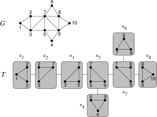
Figure 1: A graph $G$ of tree-width 2 and a tree decomposition $({\mathcal{X}},T)$ of width $2$ for $G$.

Next we give some examples for graph classes of bounded tree-width. Trees have tree-width 1 [Bod98]. Series parallel graphs have tree-width at most 2 [WC83]. Halin graphs have tree-width at most 3 [Bod88b]. $k$-outerplanar graphs have tree-width at most $3k-1$ [Bod88b]. A more detailed overview on graph classes of bounded tree-width can be found in [Bod86], [Bod88b].

On the other hand, the tree-width of complete graphs and thus of co-graphs (which are defined in Section 4.3) is not bounded [Bod98].

Two more recent parameters are clique-width and NLC-width, which are originally defined for labeled graphs.

Let $[k]:=\{1,\ldots,k\}$ be the set of all integers between $1$ and $k$. We work with finite undirected labeled graphs $G=(V_{G},E_{G},\mbox{lab}_{G})$, where $V_{G}$ is a finite set of vertices labeled by some mapping $\mbox{lab}_{G}:V_{G}\to[k]$ and $E_{G}\subseteq\{\{u,v\}\mid u,v\in V_{G},u\not=v\}$ is a finite set of edges. A labeled graph $J=(V_{J},E_{J},\mbox{lab}_{J})$ is a subgraph of $G$ if $V_{J}\subseteq V_{G}$, $E_{J}\subseteq E_{G}$ and $\mbox{lab}_{J}(u)=\mbox{lab}_{G}(u)$ for all $u\in V_{J}$. $J$ is an induced subgraph of $G$ if additionally $E_{J}=\{\{u,v\}\in E_{G}\mid u,v\in V_{J}\}$. The labeled graph consisting of a single vertex labeled by $a\in[k]$ is denoted by $\bullet_{a}$.

The notion of clique-width of labeled graphs is defined by Courcelle and Olariu in [CO00] as follows.

Definition 2.2 ($\mbox{CW}_{k}$, clique-width, [CO00])

Let $k$ be some positive integer. The class $\mbox{CW}_{k}$ of labeled graphs is recursively defined as follows.

• The single vertex $\bullet_{a}$ labeled by some $a\in[k]$ is in $\mbox{CW}_{k}$.

• Let $G\in\mbox{CW}_{k}$ and $J\in\mbox{CW}_{k}$ be two vertex disjoint labeled graphs. Then $G\oplus J:=(V^{\prime},E^{\prime},\mbox{lab}^{\prime})$ defined by $V^{\prime}:=V_{G}\cup V_{J}$, $E^{\prime}:=E_{G}\cup E_{J}$, and

  $$\mbox{lab}^{\prime}(u)\ :=\ \left\{\begin{array}[]{ll}\mbox{lab}_{G}(u)&\mbox{if }u\in V_{G}\\ \mbox{lab}_{J}(u)&\mbox{if }u\in V_{J}\\ \end{array}\right.,\ {\rm{for~{}all~{}}}u\in V^{\prime}$$

  is in $\mbox{CW}_{k}$.

• Let $a,b\in[k]$ be two distinct integers and $G\in\mbox{CW}_{k}$ be a labeled graph then

  • $\rho_{a\rightarrow b}(G):=(V_{G},E_{G},\mbox{lab}^{\prime})$ defined by

    $$\mbox{lab}^{\prime}(u)\ :=\ \left\{\begin{array}[]{ll}\mbox{lab}_{G}(u)&\mbox{if }\mbox{lab}_{G}(u)\not=a\\ b&\mbox{if }\mbox{lab}_{G}(u)=a\\ \end{array}\right.,\ {\rm{for~{}all~{}}}u\in V_{G}$$

    is in $\mbox{CW}_{k}$ and

  • $\eta_{a,b}(G)\ :=\ (V_{G},E^{\prime},\mbox{lab}_{G})$ defined by

    $$E^{\prime}:=E_{G}\cup\{\{u,v\}\mid u,v\in V_{G},~{}u\not=v,~{}\mbox{lab}(u)=a,~{}\mbox{lab}(v)=b\}$$

    is in $\mbox{CW}_{k}$.

The clique-width of a labeled graph $G$ (denoted by $\mbox{clique-width}(G)$) is the least integer $k$ such that $G\in\mbox{CW}_{k}$.

The notion of NLC-width of labeled graphs is defined by Wanke in [Wan94] as follows.

Definition 2.3 ($\mbox{NLC}_{k}$, NLC-width, [Wan94])

Let $k$ be some positive integer. The graph class $\mbox{NLC}_{k}$ of labeled graphs is recursively defined as follows.

1. The single vertex graph $\bullet_{a}$ for some $a\in[k]$ is in $\mbox{NLC}_{k}$.

2. Let $G=(V_{G},E_{G},\mbox{lab}_{G})\in\mbox{NLC}_{k}$ and $J=(V_{J},E_{J},\mbox{lab}_{J})\in\mbox{NLC}_{k}$ be two vertex disjoint labeled graphs and $S\subseteq[k]^{2}$ be a relation, then $G\times_{S}J:=(V^{\prime},E^{\prime},\mbox{lab}^{\prime})$ defined by $V^{\prime}:=V_{G}\cup V_{J}$,

   $$E^{\prime}:=E_{G}\cup E_{J}\cup\{\{u,v\}\mid u\in V_{G},~{}v\in V_{J},~{}(\mbox{lab}_{G}(u),\mbox{lab}_{J}(v))\in S\},$$

   and

   $$\mbox{lab}^{\prime}(u)\ :=\ \left\{\begin{array}[]{ll}\mbox{lab}_{G}(u)&\mbox{if }u\in V_{G}\\ \mbox{lab}_{J}(u)&\mbox{if }u\in V_{J}\\ \end{array}\right.,~{}\forall u\in V^{\prime}$$

   is in $\mbox{NLC}_{k}$.

3. Let $G=(V_{G},E_{G},\mbox{lab}_{G})\in\mbox{NLC}_{k}$ be a labeled graph and $R:[k]\to[k]$ be a function, then $\circ_{R}(G):=(V_{G},E_{G},$ $\mbox{lab}^{\prime})$ defined by $\mbox{lab}^{\prime}(u):=R(\mbox{lab}_{G}(u)),~{}\forall u\in V_{G}$ is in $\mbox{NLC}_{k}$.

The NLC-width of a labeled graph $G$ (denoted by $\mbox{NLC-width}(G)$) is the least integer $k$ such that $G\in\mbox{NLC}_{k}$.

An expression built with the operations $\bullet_{a},\oplus,\rho_{a\rightarrow b},\eta_{a,b}$ for integers $a,b\in[k]$ is called a clique-width $k$-expression. An expression $X$ built with the operations $\bullet_{a},\times_{S},\circ_{R}$ for $a\in[k]$, $S\subseteq[k]^{2}$, and $R:[k]\to[k]$ is called an NLC-width $k$-expression. The clique-width (the NLC-width) of an unlabeled graph $G=(V,E)$ is the smallest integer $k$, such that there is some mapping $\mbox{lab}:V\to[k]$ such that the labeled graph $(V,E,\mbox{lab})$ has clique-width at most $k$ (NLC-width at most $k$, respectively). The graph defined by expression $X$ is denoted by $\mbox{val}(X)$. By the definition of $k$-expressions it is easy to verify that graphs of bounded clique-width and graphs of bounded NLC-width are closed under taking induced subgraphs.

Every clique-width $k$-expression $X$ has by its recursive definition a tree structure that is called the clique-width $k$-expression-tree $T$ for $X$. $T$ is an ordered rooted tree whose leaves correspond to the vertices of graph $\mbox{val}(X)$ and the inner nodes correspond to the operations of $X$, see [EGW03]. In the same way we define the NLC-width $k$-expression-tree for every NLC-width $k$-expression, see [GW00]. If integer $k$ is known from the context or irrelevant for the discussion, then we sometimes use the simplified notion expression-tree for the notion $k$-expression-tree.

The following example shows that every clique $K_{n}$, $n\geq 1$, has clique-width 2 and NLC-width 1 and that every path $P_{n}$ has clique-width at most 3 and NLC-width at most 3.

Example 2.4

1. Every clique $K_{n}=(\{v_{1},\ldots,v_{n}\},\{\{v_{i},v_{j}\}~{}|~{}1\leq i<j\leq n\})$, $n\geq 2$, has clique-width 2, by the following recursively defined expressions $X_{K_{n}}$.

   $$\begin{array}[]{lcl}X_{K_{2}}&:=&\eta_{1,2}(\bullet_{1}\oplus\bullet_{2})\\ X_{K_{n}}&:=&\eta_{1,2}(\rho_{2\to 1}(X_{K_{n-1}})\oplus\bullet_{2}),{\rm if}~{}n\geq 3\end{array}$$

2. Every path $P_{n}=(\{v_{1},\ldots,v_{n}\},\{\{v_{1},v_{2}\},\ldots,\{v_{n-1},v_{n}\}\})$ has clique-width at most 3, by the following recursively defined expressions $X_{P_{n}}$.

   $$\begin{array}[]{lcl}X_{P_{3}}&:=&\eta_{2,3}(\eta_{1,2}(\bullet_{1}\oplus\bullet_{2})\oplus\bullet_{3})\\ X_{P_{n}}&:=&\eta_{2,3}(\rho_{3\to 2}(\rho_{2\to 1}(X_{P_{n-1}}))\oplus\bullet_{3}),{\rm if}~{}n\geq 4\end{array}$$

3. Every clique $K_{n}$, $n\geq 1$, has NLC-width 1, by the following recursively defined expressions $X_{K_{n}}$.

   $$\begin{array}[]{lcl}X_{K_{1}}&:=&\bullet_{1}\\ X_{K_{n}}&:=&X_{K_{n-1}}\times_{\{(1,1)\}}\bullet_{1},{\rm if}~{}n\geq 2\end{array}$$

4. Every path $P_{n}$ has NLC-width at most 3, by the following recursively defined expressions $X_{P_{n}}$.

   $$\begin{array}[]{lcl}X_{P_{3}}&:=&(\bullet_{1}\times_{\{(1,2)\}}\bullet_{2})\times_{\{(2,3)\}}\bullet_{3}\\ X_{P_{n}}&:=&\circ_{\{(1,1),(2,1),(3,2)\}}(X_{P_{n-1}})\times_{\{(2,3)\}}\bullet_{3},{\rm if}~{}n\geq 4\end{array}$$

Next we give some examples for graph classes of bounded clique-width. Distance hereditary graphs have clique-width at most 3 [GR00]. Co-graphs, i.e. $P_{4}$-free graphs have clique-width at most 2 [CO00]. Further, many graph classes defined by a limited number of $P_{4}$ have bounded clique-width, e.g. $P_{4}$-reducible graphs, $P_{4}$-sparse graphs, $P_{4}$-tidy, and $(q,t)$-graphs [CMR00, MR99]. A recent survey on graph classes of bounded clique-width is given in [KLM07].

On the other hand, the clique-width of permutation graphs, interval graphs, grids and planar graphs is not bounded [GR00].

2.2 Relations between graph parameters

Next we briefly survey the relation between tree-width, clique-width, and NLC-width.

Theorem 2.5 ([Joh98])

Every graph of clique-width $k$ has NLC-width at most $k$, and every graph of NLC-width at most $k$ has clique-width at most $2k$.

Thus we conclude that a set of graphs has bounded clique-width if and only if it has bounded NLC-width. Both concepts are useful, because it is sometimes much more comfortable to use NLC-width expressions instead of clique-width expressions and vice versa, respectively, see Chapter 4.

It is well known that every graph of bounded tree-width also has bounded clique-width, see [CO00, CR05, Wan94]. The best known bound is the following one shown by Corneil and Rotics.

Theorem 2.6 ([CR05])

Let $G$ be a graph of tree-width $k$, then $G$ has clique-width at most $3\cdot 2^{k-1}$.

Conversely, the tree-width of a graph can not be bounded in its clique-width in general. This shows e.g. the set of all complete graphs ($K_{n}$ has clique-width 2 and tree-width $n-1$). Under the additional assumption that we restrict to graphs that do not contain arbitrary large complete bipartite graphs $K_{n,n}$, the tree-width of a graph can be bounded in its clique-width [GW00]. Thus, if we restrict to graphs of bounded vertex degree or planar graphs, a set of graphs has bounded tree-width or bounded path-width if and only if it has bounded clique-width or bounded linear clique-width, respectively.

A further very useful and interesting relation between tree-width and clique-width has been shown using the concept of line graphs. A set of graphs has bounded tree-width if and only if the corresponding set of line graphs has bounded clique-width [GW07].

2.3 Definitions of basic graph parameters

Next we give definitions for the four basic graph parameters independence number, clique number, chromatic number, and clique covering number.

Problem 2.7 (Independent Set, [GT20] in [GJ79])

Instance:

A graph $G=(V_{G},E_{G})$ and a positive integer $s\leq|V_{G}|$.

Question:

Is there an independent set of size at least $s$ in $G$, i.e. a subset $V^{\prime}\subseteq V_{G}$, such that $|V^{\prime}|\geq s$ and no two vertices of $V^{\prime}$ are joined by an edge in $E_{G}$?

The maximum value $s$ such that $G$ has an independent set of size $s$ is denoted as the independence number of graph $G$, denoted by $\alpha(G)$.

Problem 2.8 (Clique, [GT19] in [GJ79])

Instance:

A graph $G=(V_{G},E_{G})$ and a positive integer $s\leq|V_{G}|$.

Question:

Is there a clique of size at least $s$ in $G$, i.e. a subset $V^{\prime}\subseteq V_{G}$, such that $|V^{\prime}|\geq s$ and every two vertices of $V^{\prime}$ are joined by an edge in $E_{G}$?

The maximum value $s$ such that $G$ has a clique of size $s$ is denoted as the clique number of $G$, denoted by $\omega(G)$.

Problem 2.9 (Partition Into Independent Sets, [GT4] in [GJ79])

Instance:

A graph $G=(V_{G},E_{G})$ and a positive integer $s\leq|V_{G}|$.

Question:

Is there a partition of $V_{G}$ into $s$ disjoint sets $V_{1},\ldots,V_{s}$ such that $V_{1}\cup\cdots\cup V_{s}=V_{G}$ and no set $V_{t}$, $1\leq t\leq s$, has two adjacent vertices?

The minimum value $s$ such that $G$ has a partition into $s$ independent sets is denoted as the chromatic number of $G$, denoted by $\chi(G)$. Equivalently and motivating the notation chromatic number, $\chi(G)$ is the least integer $s$, such that there is a vertex coloring $\text{col}:V_{G}\to\{1,\ldots,s\}$ such that for every pair of adjacent vertices $v_{1},v_{2}\in V_{G}$, $v_{1}\neq v_{2}$, it holds $\text{col}(v_{1})\neq\text{col}(v_{2})$.

Problem 2.10 (Partition Into Cliques, [GT15] in [GJ79])

Instance:

A graph $G=(V_{G},E_{G})$ and a positive integer $s\leq|V_{G}|$.

Question:

Is there a partition of $V_{G}$ into $s$ disjoint sets $V_{1},\ldots,V_{s}$ such that $V_{1}\cup\cdots\cup V_{s}=V_{G}$ and every set $V_{t}$, $1\leq t\leq s$, induces a complete subgraph?

The minimum value $s$ such that $G$ has a partition into $s$ cliques is denoted as the clique covering number of $G$, denoted by $\theta(G)$.

The graph parameters $\alpha$, $\omega$, $\chi$, and $\theta$ play an important rule in the field of the research of perfect graphs. One of the most famous characterizations for these graphs is that a graph $G$ is perfect if and only if for every induced subgraph $H$ of $G$ it holds $\omega(H)=\chi(H)$, if and only if for every induced subgraph $H$ of $G$ it holds $\alpha(H)=\theta(H)$. Examples for perfect graph classes are bipartite graphs, chordal graphs, and co-graphs, see [Hou06] for an overview. A further characterization for perfect graphs is that a graph $G$ is perfect if and only if $G$ contains no $C_{2n+1}$ and no $\overline{C_{2n+1}}$ as an induced subgraph. Since the cycle on 5 vertices has tree-width 2 and clique-width 3, we conclude that graphs of tree-width at most $k$ and graphs of clique-width at most $k$ are not perfect for every integer $k\geq 2$ and $k\geq 3$, respectively.

In Table 1 we survey the results of this paper.

	$\alpha$		$\omega$		$\chi$		$\theta$
trees/forest	Lin	Thm 3.7	Lin	folk	Lin	folk	Lin	Thm 3.8
$\mbox{TW}_{k}$	Lin	Thm 3.3	Lin	Thm 3.4	P	Thm 3.5	P	Thm 3.6
co-graphs	Lin	Thm 4.7	Lin	Thm 4.8	Lin	Thm 4.9	Lin	Thm 4.10
$\mbox{CW}_{k}$	Lin	Thm 4.3	Lin	Thm 4.4	P	Thm 4.5	P	Thm 4.6

Table 1: Overview on the time complexity of computing $\alpha$, $\omega$, $\chi$, and $\theta$ on special graph classes.

3 Tree-width and polynomial time algorithms

3.1 A general framework

In order to solve hard problems restricted to graph classes of bounded tree-width, we will perform a dynamic programming scheme on the tree decomposition introduced in Definition 2.1.

Although computing the tree-width of a given graph is NP-complete [ACP87], for every fixed integer $k$, the problem to decide whether a given graph $G$ has tree-width at most $k$ can be solved in linear time and in the case of a positive answer a tree decomposition of width $k$ for $G$ can be found in the same time [Bod96]. For the purpose of convenience we want to restrict our algorithms to special binary decompositions which is always possible by the following theorem.

Theorem 3.1 ([Klo94])

Let $G$ be a graph of tree-width $k$. Then $G$ has a tree decomposition $({\mathcal{X}}=\{X_{u}\mid~{}u\in V_{T}\},~{}T=(V_{T},E_{T}))$ of width $k$, such that a root $r$ of $T$ can be chosen such that the following five conditions are fulfilled.

1. Every node of $T$ has at most two children.

2. If a node $u$ of $T$ has two children $v$ and $w$, then $X_{u}=X_{v}=X_{w}$. In this case $u$ is called a join node.

3. If a node $u$ of $T$ has one child $v$, then one of the following tow conditions hold true.

   1. $|X_{u}|=|X_{v}|+1$ and $X_{v}\subset X_{u}$. In this case $u$ is called an introduce node.

   2. $|X_{u}|=|X_{v}|-1$ and $X_{u}\subset X_{v}$. In this case $u$ is called a forget node.

4. If a node $u$ is a leaf of $T$, then $|X_{u}|=1$.

5. $|V_{T}|\in O(k\cdot|V_{G}|)$.

A tree decomposition which fulfills the five conditions of Theorem 3.1 is called a nice tree decomposition and can be found in linear time [Klo94]. Let $G$ be a graph of tree-width $k$ and $({\mathcal{X}}=\{X_{u}\mid u\in V_{T}\},~{}T=(V_{T},E_{T}))$ tree decomposition with root $r$ for $G$. For some node $u$ of $T$ we define $T_{u}$ as the subtree of $T$ rooted at $u$ and by ${\mathcal{X}}_{u}$ the set of all $X_{v}$, $v\in V_{T_{u}}$. Further by $G_{u}$ we define the subgraph of $G$ which is defined by all nodes in sets $X_{v}$ where $v=u$ or $v$ is a child of $u$ in $T$, i.e. $G_{u}$ is defined by tree decomposition $({\mathcal{X}}_{u},T_{u})$. The sets $X_{u}\in{\mathcal{X}}$ will be denoted as bags.

Our solutions are based on a separator property of the vertices of graphs given by a tree decomposition $({\mathcal{X}},T)$ of width at most $k$. Let $u$, $w$ be two nodes of $T$ and $v_{1}\in X_{u}$, $v_{2}\in X_{w}$ two vertices of the graph $G$ defined by decomposition $({\mathcal{X}},T)$. If there exists some node $s$ of $T$ on the path from $u$ to $w$ in $T$ such that $v_{1}\not\in X_{s}$ and $v_{2}\not\in X_{s}$, then $v_{1}$ and $v_{2}$ are not adjacent in $G$, see Fig. 2. Thus the at most $k+1$ vertices of bag $X_{s}$ separate the vertices in bags below $X_{s}$ from the remaining vertices of $G$.

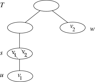
Figure 2: Separator property of some graph $G$ defined by tree decompositions $({\mathcal{X}},T)$. Let $u,w\in V_{T}$ and $v_{1}\in X_{u}$, $v_{2}\in X_{w}$ be two vertices of graph $G$. If $v_{1}\not\in X_{s}$ and $v_{2}\not\in X_{s}$, we know that vertices $v_{1}$ and $v_{2}$ are not adjacent in $G$.

In order to solve graph problems on tree-width bounded graphs we will use the following bottom up dynamic programming scheme.

Theorem 3.2

Let $\Pi$ be a graph problem and $k$ be a positive integer. If there is a mapping $F$ that maps every tree-decomposition $({\mathcal{X}}=\{X_{u}\mid~{}u\in V_{T}\},~{}T=(V_{T},E_{T}))$ with root $r$ of width $k$ onto some structure $F(r)$, such that for all nodes $v$,$w$ of $T$,

1. the size of $F(v)$ is polynomially bounded in the size of $({\mathcal{X}}_{v},T_{v})$,

2. the answer to $\Pi$ for $G_{v}$ is computable in polynomial time from $F(v)$,

3. for every leaf $u$ of $T$ structure $F(u)$ is computable in time $O(1)$,

4. for every join node $u$ with children $v,w$ structure $F(u)$ is computable in polynomial time from $F(v)$ and $F(w)$, and

5. for every introduce node and every forget node $u$ with child $v$ structure $F(u)$ is computable in polynomial time from $F(v)$.

Then for every decomposition $({\mathcal{X}},T)$ of width $k$, the answer to $\Pi$ for graph $G_{r}$ is computable in polynomial time from decomposition $({\mathcal{X}},T)$.

There are further dynamic programming approaches to solve hard problems on tree-width bounded graphs. For example in [AP89] the perfect elimination order of the vertices of a partial $k$-tree is used to solve hard problems on tree-width bounded graphs.

3.2 Computing $\alpha$, $\omega$, $\chi$, and $\theta$ on graphs of bounded tree-width

We next apply the general scheme of Theorem 3.2 for computing the four basic graph parameters $\alpha$, $\omega$, $\chi$, and $\theta$ on graphs of bounded tree-width in polynomial time.

3.2.1 Independence number

First we consider the problem of finding the size of a maximum independent set (Problem 2.7) in a graph given by some tree decomposition.

Let $({\mathcal{X}}=\{X_{u}\mid u\in V_{T}\},~{}T=(V_{T},E_{T}))$ be a tree decomposition for some graph $G$ of width $k$ with root $r$. For every node $u$ of $T$ we define a $2^{k+1}$-tuple $F(u)$ which contains for every subset $X\subseteq X_{u}$ an integer $a_{X}$, i.e. $F(u)=(a_{X}~{}|~{}X\subseteq X_{u})$. The value of $a_{X}$ denotes the size of a maximum independent set $U\subseteq V_{G_{u}}$ in graph $G_{u}$ such that $U\cap X_{u}=X$. Note that because of our separator property, vertices from $U-X$ will not get any further edges in bag $X_{u}$ or some bag $X_{w}$ for some node $w$ which is not a child of $u$ in $T$.

Then $F(r)$ is bounded in $k$ independently of the size of $({\mathcal{X}},T)$, because by the definition every bag contains at most $k+1$ vertices and thus $F(r)$ has at most $2^{k+1}$ entries. The following observations show that for every leaf $u$ of $T$ structure $F(u)$ is computable in time $O(2^{k+1})$, for every join node $u$ with children $v$,$w$ structure $F(u)$ is computable in time $O(2^{k+1})$ from $F(v)$ and $F(w)$, and for every introduce node and every forget node $u$ with child $v$ structure $F(u)$ is computable in time $O(2^{k+1})$ from $F(v)$.

1. If $u$ is a leaf of $T$, such that $X_{u}=\{v_{1}\}$ for some $v_{1}\in V_{G}$. We define $F(u):=(a_{\emptyset}=0,a_{\{v_{1}\}}=1)$.

2. If $u$ is a join node with children $v,w$ of $T$. Let $F(v)=(a_{X}~{}|~{}X\subseteq X_{v})$, $F(w)=(b_{X}~{}|~{}X\subseteq X_{w})$, and $i_{X}$ be the size of the largest independent set in $X\subseteq X_{u}$. Then we define $F(u):=(c_{X}~{}|~{}X\subseteq X_{u})$, where $\forall X\subseteq X_{u}$, $c_{X}:=a_{X}+b_{X}-i_{X}$.

3. If $u$ is an introduce node with child $v$ of $T$, such that $X_{u}-X_{v}=\{v^{\prime}\}$ for some $v^{\prime}\in V_{G}$. Let $F(v)=(a_{X}~{}|~{}X\subseteq X_{v})$. Then we define $F(u)=(b_{X}~{}|~{}X\subseteq X_{u})$, where $\forall X\subseteq X_{v}$, $b_{X}:=a_{X}$ and

   $$b_{X\cup\{v^{\prime}\}}:=\left\{\begin{array}[]{ll}a_{X}+1&\text{if $v^{\prime}$ is not adjacent to some vertex from }X\\ -\infty&\text{else }\\ \end{array}\right.$$

4. If $u$ is a forget node with child $v$ of $T$, such that $X_{v}-X_{u}=\{v^{\prime}\}$ for some $v^{\prime}\in V_{G}$. Let $F(v)=(a_{X}~{}|~{}X\subseteq X_{v})$. Then we define $F(u):=(b_{X}~{}|~{}X\subseteq X_{u})$, where $\forall X\subseteq X_{u}$, $b_{X}:=\max\{a_{X},a_{X\cup\{v^{\prime}\}}\}$.

After a dynamic programming computation of $F(r)$ we can easily compute the size of a maximum independent set in graph $G$ by $\alpha(G):=\max_{a\in F(r)}a$

Theorem 3.3

The independence number of a graph of bounded tree-width can be computed in linear time.

In [Chl02] it is shown that for every graph $G$ the value of $|V_{G}|-\mbox{tree-width}(G)$ always is an upper bound for the independence number $\alpha(G)$.

3.2.2 Clique number

Next we consider the problem of finding the size of a maximum clique (Problem 2.8) in a graph given by some tree decomposition.

Let $G$ be some graph and $({\mathcal{X}}=\{X_{u}\mid~{}u\in V_{T}\},~{}T=(V_{T},E_{T}))$ be a tree decomposition of width $k$ for $G$. In order to compute the value of $\omega(G)$ obviously a similar solution as given for independent set problem above is possible. Alternatively one could use the well known result that for every clique $C=(V_{C},E_{C})$ in graph $G$ there exists some bag $X_{u}\in{\mathcal{X}}$ such that $V_{C}\subseteq X_{u}$, see [BM93]. This allows us to compute the value of $\omega(G)$ for graph $G$ of tree-width $k$ by

$$\omega(G):=\max_{u\in V_{T}}\max_{C\subseteq X_{u}\atop{G[C]\text{~{}clique}}}|C|.$$

Theorem 3.4

The clique number of a graph of bounded tree-width can be computed in linear time.

3.2.3 Chromatic number

Further we consider the problem of finding the minimum number of independent sets (Problem 2.9) covering a graph given by some tree decomposition.

Let $({\mathcal{X}}=\{X_{u}\mid~{}u\in V_{T}\},~{}T=(V_{T},E_{T}))$ be a tree decomposition for some graph $G$ of width $k$ with root $r$. For every node $u$ of $T$, we define a set $F(u)$ which contains for every partition of $V_{G_{u}}$ into independent sets $V_{1},\ldots,V_{s}$ a $2^{k+1}$-tuple $t=(\ldots,a_{X},\ldots,a)$ which contains for every nonempty subset $X\subseteq X_{u}$ a boolean value $a_{X}$ and one integer $a$. For some disjoint partition $V_{1},\ldots,V_{s}$ of $V_{G_{u}}$ into independent sets, the value of $a_{X}$ is $1$, if and only if $V_{i}\cap X_{u}=X$ for some $1\leq i\leq r$ and the value of $a$ denotes the number of independent sets $V_{i}$ such that $V_{i}\cap X_{u}=\emptyset$.

Then $F(r)$ is polynomially bounded in the size of $({\mathcal{X}},T)$, because every element of $F(r)$ has $2^{k+1}$ entries, $2^{k+1}-1$ from $\{0,1\}$ and one from $\{1,\ldots,|V_{G}|\}$, i.e. $|F(r)|\leq 2^{2^{k+1}-1}\cdot|V_{G}|$. The following observations show that for every leaf $u$ of $T$ structure $F(u)$ is computable in time $O(1)$, for every join node $u$ with children $v$,$w$ structure $F(u)$ is computable in polynomial time from $F(v)$ and $F(w)$, and for every introduce node and every forget node $u$ with child $v$ structure $F(u)$ is computable in polynomial time from $F(v)$.

1. If $u$ is a leaf of $T$, such that $X_{u}=\{v_{1}\}$ for some $v_{1}\in V_{G}$. We define $F(u):=\{(a_{\{v_{1}\}}=1,a=0)\}$.

2. If $u$ is a join node with children $v,w$ of $T$. Then we define $F(u):=\{(\ldots,a_{X},\ldots,a+b)~{}|~{}(\ldots,a_{X},\ldots,a)\in F(v),(\ldots,b_{X},\ldots,b)\in F(w),a_{X}=b_{X},\text{for all }X\subseteq X_{u}\}$.

3. If $u$ is an introduce node with child $v$ of $T$, such that $X_{u}-X_{v}=\{v^{\prime}\}$ for some $v^{\prime}\in V_{G}$. We consider every partition of $X_{v}$ into independent sets in order to insert a new independent set which just contains vertex $v^{\prime}$ and to extend one existing independent set of a partition of $X_{v}$ by vertex $v^{\prime}$.

   Thus we define $F(u)$ as follows. For every tuple $t\in F(v)$ we insert a tuple $t^{\prime}$ into $F(u)$ which contains the same values as $t$ and additionally $a_{\{v^{\prime}\}}:=1$. Further for every tuple $t\in F(v)$ and every $X\subseteq X_{v}$ such that $a_{X}=1$ in $F(v)$ and $X\cup\{v^{\prime}\}$ is an independent set of graph $G$, we insert a tuple $t^{\prime}$ into $F(u)$ which contains the same values as $t$ but $a_{X}:=0$ and additionally $a_{X\cup\{v^{\prime}\}}:=1$. In both cases the value of $a$ of $t^{\prime}$ is the same as in $t$.

4. If $u$ is a forget node with child $v$ of $T$, such that $X_{v}-X_{u}=\{v^{\prime}\}$ for some $v^{\prime}\in V_{G}$. We know that in every partition of $X_{v}$ there is exactly one independent set $X$ which contains $v^{\prime}$. If $X$ does not contain any further vertex, we have to increase the value of $a$ in $F(u)$ by one, otherwise we know that $X-\{v^{\prime}\}$ is an independent set in $G_{u}$, i.e. $a_{X-\{v^{\prime}\}}=1$ in $F(u)$.

   Thus we define $F(u)$ as follows. For every tuple $t=(\ldots,a_{X},\ldots,a)\in F(v)$ we insert a tuple $t^{\prime}:=(\ldots,b_{X},\ldots,b)$ into $F(u)$ which is defined as follows. If $a_{\{v^{\prime}\}}=1$, then we define for every $X\subseteq X_{v}$ $b_{X-\{v^{\prime}\}}:=a_{X}$ and $b:=a+1$. Otherwise (i.e. $a_{\{v^{\prime}\}}=0$), we define for every $X\subseteq X_{v}$ $b_{X-\{v^{\prime}\}}:=a_{X}$ and $b:=a$.

Note that in all four cases set $F(u)$ has at most $2^{|X_{u}|}$ entries.

After a dynamic programming computation of $F(r)$ we can compute the chromatic number of graph $G$ by $\chi(G):=\min_{t\in F(r)}\sum_{a\in t}a$.

Theorem 3.5

The chromatic number of a graph of bounded tree-width can be computed in polynomial time.

In [Chl02] it is shown that for every graph $G$ the value of $\mbox{tree-width}(G)+1$ is always an upper bound for the chromatic number $\chi(G)$.

If we consider Problem 2.9 for the case that we look for a partition into a minimum number of independent edge sets, we obtain the graph parameter chromatic index, see [Viz64], [Gup66], which has been shown to be computable in linear time on graphs of bounded tree-width in [ZFN00].

3.2.4 Clique covering number

Further we consider the problem of finding the minimum number of cliques (Problem 2.10) covering a graph given by some tree decomposition.

Let $({\mathcal{X}}=\{X_{u}\mid~{}u\in V_{T}\},~{}T=(V_{T},E_{T}))$ be a tree decomposition for some graph $G$ of width $k$ with root $r$. We will proceed similarly to the solution given in Section 3.2.3 for computing the chromatic number. For every node $u$ of $T$, we define a set $F(u)$ which contains for every disjoint partition of $V_{G_{u}}$ into cliques $V_{1},\ldots,V_{s}$ a $2^{k+1}$-tuple $t=(\ldots,a_{X},\ldots,a)$ which contains for every nonempty subset $X\subseteq X_{u}$ a boolean value $a_{X}$ and one integer $a$. For some disjoint partition $V_{1},\ldots,V_{s}$ of $V_{G_{u}}$ into cliques, the value of $a_{X}$ is $1$, if and only if $V_{i}=X$ for some $1\leq i\leq r$ and the value of $a$ denotes the number of cliques $V_{i}$ such that $V_{i}\cap X_{u}=\emptyset$.

Then $F(r)$ is polynomially bounded in the size of $({\mathcal{X}},T)$, because $|F(r)|\leq 2^{2^{k+1}-1}\cdot|V_{G}|$. Further for every leaf $u$ of $T$ structure $F(u)$ is computable in time $O(1)$, for every join node $u$ with children $v$,$w$ structure $F(u)$ is computable in polynomial time from $F(v)$ and $F(w)$, and for every introduce node and every forget node $u$ with child $v$ structure $F(u)$ is computable in polynomial time from $F(v)$. This follows by step (1) and (2) given in Section 3.2.3 and by replacing independent set by clique in step (3) and (4) given in Section 3.2.3.

After a dynamic programming computation of $F(r)$ we can compute the clique covering number of graph $G$ by $\theta(G):=\min_{t\in F(r)}\sum_{a\in t}a$

Theorem 3.6

The clique covering number of a graph of bounded tree-width can be computed in polynomial time.

3.3 Computing $\alpha$, $\omega$, $\chi$, and $\theta$ on trees

We next show that for graphs of tree-width one, i.e. for trees, our shown algorithms can be simplified.

3.3.1 Independence number

Let $T$ be some tree. The independence number $\alpha(T)$ can be computed by $\alpha(T)=\alpha(T_{r})$, where $T_{r}$ is the corresponding rooted tree by choosing an arbitrary vertex $r$ of $T$ as a root. The value of $\alpha(T_{r})$ (and thus $\alpha(T)$) can be computed by dynamic programming as follows.

1. If $|V_{T_{r}}|=1$, i.e. $r$ is a leaf of $T_{r}$, then $\alpha(T_{r}):=1$.

2. If $|V_{T_{r}}|\geq 2$, i.e. $r$ is an inner node of $T_{r}$, then

   $$\alpha(T_{r}):=\max\{\sum_{\mbox{$c$ child of $r$}}\alpha(T_{c}),~{}1+\sum_{\mbox{$g$ grandchild of $r$}}\alpha(T_{g})\}$$

Theorem 3.7

For every tree its independence number can be computed in linear time.

3.3.2 Clique number

Obviously for every tree $T$, if $|V_{T}|=1$, then $\omega(T):=1$ and if $|V_{T}|\geq 2$, then $\omega(T):=2$.

3.3.3 Chromatic number

Obviously for every tree $T$, if $|V_{T}|=1$, then $\chi(T):=1$ and if $|V_{T}|\geq 2$, then $\chi(T):=2$, since every tree is a bipartite graph.

3.3.4 Clique covering number

Since trees are perfect, we know that for every induced subgraph $H$ of some tree $T$ it holds $\theta(H)=\alpha(H)$, and thus we can compute clique covering number $\theta(T)$ by the same algorithm as shown for $\alpha(T)$ above.

Theorem 3.8

For every tree its clique covering number can be computed in linear time.

3.4 Complement problems

Let $\Pi$ be a decision problem for graphs. We define the corresponding complement problem $\overline{\Pi}$ by

$$\overline{\Pi}:=\{\overline{G}~{}|~{}G{\rm~{}satiesfies~{}}\Pi\}.$$

For several graph problems the corresponding complement problem is also of interest. For example the complement problem of the independent set problem (Problem 2.7) is the clique problem (Problem 2.8) and the complement problem of the partition into independent sets problem (Problem 2.9) is the partition into cliques problem (Problem 2.10).

Since for some set of graphs ${\mathcal{L}}\subseteq\mbox{TW}_{k}$, the corresponding set of complement graphs $\overline{\mathcal{L}}:=\{\overline{G}~{}|~{}G\in{\mathcal{L}}\}$ not necessarily has bounded tree-width, the solvability of complement problems on tree-width bounded graphs are worthwhile to research. In [GKS00] Gupta et al. give a logical framework for solving complement problems on tree-width bounded graphs in polynomial time.

3.5 Tree-width and monadic second order logic

On graph classes of bounded tree-width, all graph properties and optimization problems which are expressible in monadic second order logic with quantifications over vertices, vertex sets, edges, and edge sets ($\text{MSO}_{2}$-logic) are decidable in linear time [CM93]. This implies the existence of linear time algorithms for computing the independence number and clique number on graphs of bounded tree-width. Note that the problems partition into independent sets and partition into cliques are not expressible in $\text{MSO}_{2}$-logic.

4 Clique-width and polynomial time algorithms

4.1 A general framework

In order to solve hard problems restricted to graph classes of bounded clique-width, we recall a dynamic programming approach on the tree structure of a clique-width or an NLC-width expression from [EGW01].

Recently it has been shown that computing the clique-width and NLC-width of a given graph is NP-hard [FRRS06, GW05]. For every fixed integer $k\leq 3$ or $k\leq 2$, the problem to decide whether a given graph has clique-width at most $k$ or NLC-width at most $k$ can be solved in polynomial time and in the case of a positive answer a $k$-expression can be constructed in the same time [CPS85, CHL⁺00, LdMR07]. For every fixed integer $k\geq 4$ or $k\geq 3$, the problem to decide whether a given graph has clique-width at most $k$ or NLC-width at most $k$ is still open. Nevertheless we can use the approximations for rank-width shown by Oum and Seymour in [OS06, Oum05, Oum06] in order to obtain approximations for clique-width and a corresponding clique-width expression. The best known result is the following.

Theorem 4.1 ([Oum06])

For every fixed integer $k$ there is a $O(|V_{G}|^{3})$ algorithm that either outputs a clique-width $(8^{k}-1)$-expression of an input graph $G$, or confirms that the clique-width of $G$ is larger that $k$.

Every clique-width $k$-expression can be transformed into an equivalent NLC-width $k$-expression within linear time [Joh98]. Thus, the last theorem implies that for every fixed integer $k$, for every set ${\mathcal{L}}\subseteq\mbox{CW}_{k}$ and every set ${\mathcal{L}}\subseteq\mbox{NLC}_{k}$, we can assume within cubic time every graph $G\in{\mathcal{L}}$ to be given with some $(8^{k}-1)$-expression.

For some node $u$ of expression-tree $T$, let $T(u)$ be the subtree of $T$ rooted at $u$. Note that tree $T(u)$ is always an expression-tree. The expression $X(u)$ defined by $T(u)$ can simply be determined by traversing the tree $T(u)$ starting from the root, where the left children are visited first. $X(u)$ defines a (possibly) relabeled induced subgraph $G[u]$ of $G$.

Our solutions are based on a neighbourhood property of the vertices of graphs given by a $k$-expression $X$ defining a corresponding $k$-expression tree $T$. For every node $u$ of $T$, the vertices of subgraph $G[u]$ form a $k$-module, i.e. every set $V_{i}=\{\mbox{lab}(v)=i~{}|~{}v\in V_{G[u]}\}$, $1\leq i\leq k$, is a module of $G[V_{G}-(V_{1}\cup\ldots\cup V_{k})\cup V_{i}]$. That is, all vertices in set $V_{i}$, $1\leq i\leq k$, will be treated equally by all operations in $T$ on the path from $u$ to the root of $T$, see Fig. 3.

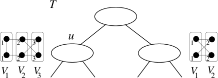
Figure 3: Neighbourhood property of graphs defined by $k$-expression tree $T$. For every node $u\in V_{T}$, the vertices of subgraph $G[u]$ can be divided with respect to their labels into at most $k$ modules $V_{1},\ldots,V_{k}$ in the graph defined by $T$.

The tree structure of such $k$-expressions can be used to solve hard problems by the following general bottom up dynamic programming scheme.

Theorem 4.2 ([EGW01])

Let $\Pi$ be a graph problem and $k$ be a positive integer. If there is a mapping $F$ that maps each clique-width $k$-expression $X$ onto some structure $F(X)$, such that for all clique-width $k$-expressions $X,Y$ and all $a,b\in[k]$

1. the size of $F(X)$ is polynomially bounded in the size of $X$,

2. the answer to $\Pi$ for $\text{val}(X)$ is computable in polynomial time from $F(X)$,

3. $F(\bullet_{a})$ is computable in time $O(1)$,

4. $F(X\oplus Y)$ is computable in polynomial time from $F(X)$ and $F(Y)$, and

5. $F(\eta_{a,b}(X))$ and $F(\rho_{a\to b}(X))$ are computable in polynomial time from $F(X)$.

Then for every clique-width $k$-expression $X$, the answer to $\Pi$ for graph $\text{val}(X)$ is computable in polynomial time from expression $X$.

Theorem 4.2 also works for NLC-width $k$-expressions built with the operations $\bullet_{a}$, $\times_{S}$, and $\circ_{R}$ instead of $\bullet_{a}$, $\oplus$, $\eta_{a,b}$, and $\rho_{a\to b}$. In this case $F(X\times_{S}Y)$ has to be computable in polynomial time from $F(X)$ and $F(Y)$, and $\circ_{R}(X)$ has to be computable in polynomial time from $F(X)$.

The given dynamic programming approach has been used in [EGW01],[GW06], [Gur07], [GK03],[KR03],[Rao07] to solve a large number of NP-complete graph problems on graph classes of bounded clique-width.

4.2 Computing $\alpha$, $\omega$, $\chi$, and $\theta$ on graphs of bounded clique-width

We next give polynomial time algorithms using for computing the four basic graph parameters $\alpha$, $\omega$, $\chi$, and $\theta$ on graphs of bounded clique-width using the general scheme of Theorem 4.2. For the sake of convenience and to emphasize the advantages of clique-width and NLC-width operations, we will use clique-width expressions for the problems independent set and partition into independent sets and NLC-width expressions for the problems clique and partition into cliques.

4.2.1 Independence number

Let us first consider the problem of computing the independence number (Problem 2.7) on graphs of bounded clique-width.

Let $G$ be a graph defined by some clique-width $k$-expression $X$. Let $F(X)$ be the $(2^{k}-1)$-tuple $(\ldots,a_{L},\ldots)$, which contains for every $L\subseteq[k]$, $L\neq\emptyset$, a non negative integer $a_{L}$, which denotes the size of a largest independent set $U$ in graph $\mbox{val}(X)$ such that $\{\mbox{lab}(u)~{}|~{}u\in U\}=L$.

Then $F(X)$ is bounded in $k$ independently of the size of $X$, because $F(X)$ has at exactly $2^{k}-1$ entries. The following observations show that $F(\bullet_{i})$ is computable in time $O(2^{k})$, $F(X\oplus Y)$ is computable in time $O(2^{k})$ from $F(X)$ and $F(Y)$, and $F(\eta_{i,j}(X))$ and $F(\rho_{i\to j}(X))$ are computable in time $O(2^{k})$ from $F(X)$.

1. We define $F(\bullet_{i}):=(\ldots,a_{L},\ldots)$, where $\forall L\subseteq[k]$

   $$a_{L}:=\left\{\begin{array}[]{ll}1&\text{if }L=\{i\}\\ 0&\text{if }L\neq\{i\}.\\ \end{array}\right.~{}$$

2. Let $F(X)=(\ldots,a_{L},\ldots)$ and $F(Y)=(\ldots,b_{L},\ldots)$, then we define $F(X\oplus Y):=(\ldots,c_{L},\ldots)$, where $c_{L}:=\max_{L=L_{1}\cup L_{2}}a_{L_{1}}+b_{L_{2}}$, $L_{1},L_{2}\subseteq[k]$.

3. Let $F(X)=(\ldots,a_{L},\ldots)$, then we define $F(\eta_{i,j}(X)):=(\ldots,b_{L},\ldots)$, where $\forall L\subseteq[k]$

   $$b_{L}:=\left\{\begin{array}[]{ll}a_{L}&\text{if }\{i,j\}\nsubseteq L\\ 0&\text{if }\{i,j\}\subseteq L\\ \end{array}\right.$$

4. Let $F(X)=(\ldots,a_{L},\ldots)$, then we define $F(\rho_{i\to j}(X)):=(\ldots,b_{L},\ldots)$, where $\forall L\subseteq[k]$

   $$b_{L}:=\left\{\begin{array}[]{ll}a_{L}&\text{if }i\not\in L\text{ and }j\not\in L\\ \max\{a_{L},a_{L-\{j\}\cup\{i\}}\}&\text{if }i\not\in L\text{ and }j\in L\\ 0&\text{if }i\in L\\ \end{array}\right.$$

   Obviously in graph $\mbox{val}(\rho_{i\to j}(X))$ there exists no vertex labeled by $i$, thus for every set $L$ with $i\in L$ we know that $b_{L}=0$.

After a dynamic programming computation of $F(X)$ we can compute the size of a maximum independent set in graph $\mbox{val}(X)$ by $\alpha(\mbox{val}(X)):=\max_{a\in F(X)}a$.

Theorem 4.3

The independence number of a graph of bounded clique-width can be computed in linear time, if the graph is given by some clique-width $k$-expression.

4.2.2 Clique number

Let us next consider the problem of computing the clique number (Problem 2.8).

In order have some knowledge on the order of the operations in a given expression $X$, we assume that $G$ is given by some some NLC-width $k$-expression $X$. Let $F(X)$ be the $(2^{k}-1)$-tuple $(\ldots,a_{L},\ldots)$, which contains for every $L\subseteq[k]$, $L\neq\emptyset$, a non negative integer $a_{L}$, which denotes the size of a largest clique $C$ in graph $\mbox{val}(X)$ such that $\{\mbox{lab}(v)~{}|~{}v\in C\}=L$.

Then $F(X)$ is bounded in $k$ independently from the size of $X$, because $F(X)$ has exactly $2^{k}-1$ entries. Next we will show that that $F(\bullet_{i})$ is computable in time $O(1)$, $F(X\times_{S}Y)$ is computable in $O(2^{k})$ time from $F(X)$ and $F(Y)$, and $F(\circ_{R}(X))$ is computable in time $O(2^{k})$ from $F(X)$.

1. We define $F(\bullet_{i}):=(\ldots,a_{L},\ldots)$, where $\forall L\subseteq[k]$

   $$a_{L}:=\left\{\begin{array}[]{ll}1&\text{if }L=\{i\}\\ 0&\text{if }L\neq\{i\}.\\ \end{array}\right.$$

2. Let $F(X)=(\ldots,a_{L},\ldots)$ and $F(Y)=(\ldots,b_{L},\ldots)$, then we define $F(X\times_{S}Y):=(\ldots,c_{L},\ldots)$, where the values for $c_{L}$ are defined as follows.

   We say relation $S=\{(i_{1},j_{1}),\ldots,(i_{l},j_{l})\}$ defines a join for the label sets $L_{1},L_{2}$, denoted by $L=L_{1}\uplus L_{2}$, if there is a subset $I\subseteq[l]$ such that $L_{1}=\cup_{i^{\prime}\in I}i_{i^{\prime}}$ and $L_{2}=\cup_{i^{\prime}\in I}j_{i^{\prime}}$ and $L=L_{1}\cup L_{2}$. Then we can define $\forall L\subseteq[k]$

   $$c_{L}:=\left\{\begin{array}[]{ll}\max_{L=L_{1}\uplus L_{2}}\{a_{L_{1}}+b_{L_{2}},a_{L},b_{L}\}&\text{if there exists some }L_{1}\uplus L_{2}=L\\ \max\{a_{L},b_{L}\}&\text{else }\\ \end{array}\right.$$

3. Let $F(X)=(\ldots,a_{L},\ldots)$, then we define $F(\circ_{R}(X)):=(\ldots,b_{L},\ldots)$, where $\forall L\subseteq[k]$

   $$b_{L}:=\left\{\begin{array}[]{ll}\max_{R(L^{\prime})=L}a_{L^{\prime}}&\text{if there exists some }L^{\prime}\subseteq[k]:R(L^{\prime})=L\\ 0&\text{else }\\ \end{array}\right.$$

After a dynamic programming computation of $F(X)$ we can compute the size of a maximum clique in graph $\mbox{val}(X)$ by $\omega(\mbox{val}(X)):=\max_{a\in F(X)}a$.

Theorem 4.4

The clique number of a graph of bounded clique-width can be computed in linear time, if the graph is given by some $k$-expression.

4.2.3 Chromatic number

Next we consider the problem of computing the chromatic number (Problem 2.9) on graphs of bounded clique-width.

Let $G$ be a graph given by some clique-width $k$-expression $X$. For a disjoint partition of $V_{G}$ into independent sets $V_{1},\ldots,V_{r}$ let ${\mathcal{M}}$ be the multi set $\langle\mbox{lab}(V_{1}),\ldots,\mbox{lab}(V_{r})\rangle$. Let $F(X)$ be the set of all mutually different multi sets ${\mathcal{M}}$ for all disjoint partitions of vertex set $V_{G}$ into independent sets.

Then $F(X)$ is polynomially bounded in the size of $X$, because $F(X)$ has at most $(|V_{G}|+1)^{2^{k}-1}$ mutually different multi sets each with at most $|V_{G}|$ nonempty subsets of $[k]$. The following observations show that $F(\bullet_{i})$ is computable in time $O(1)$, $F(X\oplus Y)$ is computable in polynomial time from $F(X)$ and $F(Y)$, and $F(\eta_{i,j}(X))$ and $F(\rho_{i\to j}(X))$ are computable in polynomial time from $F(X)$.

1. We define $F(\bullet_{i}):=\{\langle\{i\}\rangle\}$

2. Starting with set $D:=\{\langle\rangle\}\times F(X)\times F(Y)$ extend $D$ by all triples that can be obtained from some triple $({\mathcal{M}},{\mathcal{M}}^{\prime},{\mathcal{M}}^{\prime\prime})\in D$ by removing a set $L^{\prime}$ from ${\mathcal{M}}^{\prime}$ or a set $L^{\prime\prime}$ from ${\mathcal{M}}^{\prime\prime}$ and inserting it into ${\mathcal{M}}$, or by removing both sets and inserting $L^{\prime}\cup L^{\prime\prime}$ into ${\mathcal{M}}$.

   We define $F(X\oplus Y):=\{{\mathcal{M}}\mid~{}({\mathcal{M}},\langle\rangle,\langle\rangle)\in D\}$.

   $D$ gets at most $(|V_{G}|+1)^{3(2^{k}-1)}$ triples and thus is computable in polynomial time.

3. We define $F(\eta_{i,j}(X)):=\{\langle L_{1},\ldots,L_{r}\rangle\in F(X)\mid\{i,j\}\not\subseteq L_{t}~{}\text{for}~{}t=1,\ldots,r\}$.

4. We define $F(\rho_{i\to j}(X)):=\{\langle\rho_{i\to j}(L_{1}),\ldots,\rho_{i\to j}(L_{r})\rangle\mid\langle L_{1},\ldots,L_{r}\rangle\in F(X)\}$.

   For a relabeling $\rho_{i\to j}$ let $R_{i\to j}:[k]\to[k]$ be defined by $R_{i\to j}(t):=t$ if $t\not=i$, and $R_{i\to j}(t):=j$ if $t=i$. For $L\subseteq[k]$ let $\rho_{i\to j}(L):=\{R_{i\to j}(t)~{}|~{}t\in L\}$.

There is a partition of the vertex set of $\text{val}(X)$ into $r$ independent sets if and only if there is some ${\mathcal{M}}\in F(X)$ consisting of $r$ label sets. The chromatic number of graph $\text{val}(X)$ can be obtained by $\chi(\mbox{val}(X)):=\min_{{\mathcal{M}}\in F(X)}|{\mathcal{M}}|$.

Theorem 4.5

The chromatic number of a graph of bounded clique-width can be computed in polynomial time.

The time complexity of computing the graph parameter chromatic index (minimum number of colors needed to color the edges of a given graph) is open up to now even for co-graphs.

4.2.4 Clique covering number

Finally we consider the problem of computing the clique covering number (Problem 2.10) on graphs of bounded clique-width..

Let $G$ be a graph given by some NLC-width $k$-expression $X$. For a disjoint partition of $V_{G}$ into cliques $V_{1},\ldots,V_{r}$ let ${\mathcal{M}}$ be the multi set $\langle\mbox{lab}(V_{1}),\ldots,\mbox{lab}(V_{r})\rangle$. Let $F(X)$ be the set of all mutually different multi sets ${\mathcal{M}}$ for all disjoint partitions of vertex set $V_{G}$ into cliques.

Then $F(X)$ is polynomially bounded in the size of $X$, because $F(X)$ has at most $(|V_{G}|+1)^{2^{k}-1}$ mutually different multi sets each with at most $|V_{G}|$ nonempty subsets of $[k]$. The following observations show that $F(\bullet_{i})$ is computable in time $O(1)$, $F(X\times_{S}Y)$ is computable in polynomial time from $F(X)$ and $F(Y)$, and $F(\circ_{R}(X))$ is computable in polynomial time from $F(X)$.

1. We define $F(\bullet_{i}):=\{\langle\{i\}\rangle\}$

2. In order to compute $F(X\times_{S}Y)$ from $F(X)$ and $F(Y)$ we start with set $D:=\{\langle\rangle\}\times F(X)\times F(Y)$ and extend $D$ by all triples that can be obtained from some triple $({\mathcal{M}},{\mathcal{M}}^{\prime},{\mathcal{M}}^{\prime\prime})\in D$ by removing a set $L^{\prime}$ from ${\mathcal{M}}^{\prime}$ or a set $L^{\prime\prime}$ from ${\mathcal{M}}^{\prime\prime}$ and inserting it into ${\mathcal{M}}$, or if $S$ defines a join for the label sets $L^{\prime},L^{\prime\prime}$ (defined in Section 4.2.2) by removing both sets and inserting $L^{\prime}\cup L^{\prime\prime}$ into ${\mathcal{M}}$.

   We define $F(X\times_{S}Y):=\{{\mathcal{M}}\mid~{}({\mathcal{M}},\langle\rangle,\langle\rangle)\in D\}$.

   $D$ gets at most $(|V_{G}|+1)^{3(2^{k}-1)}$ triples and thus is computable in polynomial time.

3. We define $F(\circ_{R}):=\{\langle\circ_{R}(L_{1}),\ldots,\circ_{R}(L_{r})\rangle\mid~{}\langle L_{1},\ldots,L_{r}\rangle\in F(X)\}$.

   For a relabeling $\circ_{R}$ and $L\subseteq[k]$ let $\circ_{R}(L):=\{R(t)~{}|~{}t\in L\}$.

There is a partition of the vertex set of $\text{val}(X)$ into $r$ cliques if and only if there is some ${\mathcal{M}}\in F(X)$ consisting of $r$ label sets. The clique covering number of graph $\text{val}(X)$ can be obtained by $\theta(\mbox{val}(X)):=\min_{{\mathcal{M}}\in F(X)}|{\mathcal{M}}|$.

Theorem 4.6

The clique covering number of a graph of bounded clique-width can be computed in polynomial time.

4.3 Computing $\alpha$, $\omega$, $\chi$, and $\theta$ on co-graphs

We next show that for graphs of clique-width at most 2 and graphs of NLC-width 1, i.e. for co-graphs (complement reducible graphs), our shown algorithms can be simplified. A co-graph is either

• a single vertex (denoted by $\bullet$),

• the disjoint union of two co-graphs $G_{1},G_{2}$ (denoted by $G_{1}\cup G_{2}$), or

• the join of two co-graphs $G_{1},G_{2}$, which connects every vertex of $G_{1}$ with every vertex of $G_{2}$ (denoted by $G_{1}\times G_{2}$).

Obviously for every co-graph we can define a tree structure, denoted as co-tree in [CPS85]. The leaves of the co-tree represent the vertices of the graph and the inner nodes of the co-tree correspond to the operations applied on the subexpressions defined by the two subtrees. Given some co-graph $G$ we can construct a corresponding co-tree $T_{G}$ in linear time by the results shown in [CPS85]. Using the tree structure $T_{G}$, based on the results of Corneil et al. [CLSB81], we next give simple linear time algorithms for computing $\alpha$, $\omega$, $\chi$, and $\theta$ on co-graphs.

4.3.1 Independence number

For every co-graph $G$ its independence number $\alpha(G)$ can recursively be computed as follows.

1. If $|V_{G}|=1$, then $\alpha(G):=1$.

2. If $G=G_{1}\cup G_{2}$, then $\alpha(G):=\alpha(G_{1})+\alpha(G_{2})$.

3. If $G=G_{1}\times G_{2}$, then $\alpha(G):=\max\{\alpha(G_{1}),\alpha(G_{2})\}$.

Theorem 4.7

For every co-graph its independence number can be computed in linear time.

4.3.2 Clique number

For every co-graph $G$ its clique number $\omega(G)$ can recursively be computed as follows.

1. If $|V_{G}|=1$, then $\omega(G):=1$.

2. If $G=G_{1}\cup G_{2}$, then $\omega(G):=\max\{\omega(G_{1}),\omega(G_{2})\}$.

3. If $G=G_{1}\times G_{2}$, then $\omega(G):=\omega(G_{1})+\omega(G_{2})$.

Theorem 4.8

For every co-graph its clique number can be computed in linear time.

4.3.3 Chromatic number

Since co-graphs are perfect, we know that for every induced subgraph $H$ of some co-graph $G$ it holds $\chi(H)=\omega(H)$, and thus we can compute its chromatic number $\chi(G)$ by the same algorithm as shown for $\omega(G)$ above.

Theorem 4.9

For every co-graph its chromatic number can be computed in linear time.

4.3.4 Clique covering number

Again, since co-graphs are perfect, we know that for every induced subgraph $H$ of some co-graph $G$ it holds $\theta(H)=\alpha(H)$, and thus we can compute clique covering number $\theta(G)$ by the same algorithm as shown for $\alpha(G)$ above.

Theorem 4.10

For every co-graph its clique covering number can be computed in linear time.

4.4 Complement problems

If ${\mathcal{L}}\subseteq\mbox{CW}_{k}$ or ${\mathcal{L}}\subseteq\mbox{NLC}_{k}$, then for the corresponding set of complement graphs it holds $\overline{\mathcal{L}}\subseteq\mbox{CW}_{2k}$ [CO00] or $\overline{\mathcal{L}}\subseteq\mbox{NLC}_{k}$ [Wan94], respectively. This implies that for every graph problem $\Pi$ solvable in polynomial time on clique-width bounded graphs, the corresponding complement problem $\overline{\Pi}$ is also solvable in polynomial time on clique-width bounded graphs.

For example, in order to solve the clique problem on clique-width bounded graphs one can use the data structure given in Section 4.2.2. Alternatively, form a theoretically point of view, one could transform a given clique-width $k$-expression $X$ for some given graph $G$ into a clique-width $2k$-expression $X^{\prime}$ for its complement graph $\overline{G}$, and apply the algorithm for the independent set problem shown in Section 4.2.1 on $X^{\prime}$ in order to obtain the value of $\alpha(\overline{G})=\omega(G)$. The same holds true for the solution of the partition into cliques problem on clique-width bounded graphs given in Section 4.2.4. We can apply the algorithm for the partition into independent sets problem in Section 4.2.3 on an expression for the complement graph in order to obtain the value of $\chi(\overline{G})=\theta(G)$.

From a practical point of view, one should prefer the solutions using a $k$-expression instead of those using a $2k$-expression, since the clique-width of the input graph occurs as an exponent in the running time of our fpt algorithms.

4.5 Clique-width and monadic second order logic

On graph classes of bounded clique-width, all graph properties and optimization problems which are expressible in monadic second order logic with quantifications over vertices and vertex sets ($\mbox{MSO}_{1}$-logic) are decidable in linear time if a clique-width expression for the graph is given as an input [CMR00]. This also implies the existence of linear time algorithms for computing the independence number and clique number on graphs of bounded clique-width if a clique-width expression for the graph is given as an input. Note that the problems partition into independent sets and partition into cliques are not expressible in $\mbox{MSO}_{1}$-logic.

5 Conclusions

Let us briefly discuss two further well known graph parameters which can be computed in polynomial time on graphs of bounded tree-width and graphs of bounded clique-width.

A dominating set for some graph $G$ is a subset $S\subseteq V_{G}$, such that every vertex of $V_{G}-S$ is adjacent to at least one vertex from $S$. The minimum value $s$ such that $G$ has a dominating set $S\subseteq V_{G}$ of size $s$ is denoted as the dominating number of graph $G$, denoted by $\gamma(G)$.

In [AP89] it is shown that the dominating number of a graph of bounded tree-width can be computed in linear time. Further in [Rao07] it is shown that the dominating number of a graph of bounded clique-width can be computed in polynomial time.

A vertex cover for some graph $G$ is a subset $S\subseteq V_{G}$, such that every edge of $G$ has at least one endpoint in $S$. The minimum value $s$ such that $G$ has a vertex cover $S\subseteq V_{G}$ of size $s$ is denoted as the vertex cover number of graph $G$, denoted by $\tau(G)$.

Gallai has shown in [Gal59] the following relation between the size of a minimal vertex cover and maximum independent set of some graph $G$

$$\tau(G)+\alpha(G)=|V_{G}|,$$ (1)

which implies by Theorem 3.3 that the vertex cover number of a graph of bounded tree-width can be computed in linear time. For the same reason by Theorem 4.3 the vertex cover number of a graph of bounded clique-width can be computed in linear time, if the graph is given by some clique-width $k$-expression.

In this paper we have compared and illustrated how to use the tree structure of graphs of bounded tree-width and graphs of bounded clique-width to give two general dynamic programming schemes to solve problems along a tree decomposition and along a clique-width expression. Let us finally emphasize that both approaches are useful. On the one hand, clique-width allows to define larger classes of graphs of bounded width than tree-width. On the other hand, there are graph problems which remain NP-complete on graphs of bounded clique-width, but which are fixed-parameter tractable on graphs of bounded tree-width, such as the vertex disjoint path problem which is discussed in [GW06]. Further the tool of monadic second order logic allows to define provable larger classes of problems which are solvable on tree-width bounded graph classes than on clique-width bounded graph classes, see [CMR00].

References

- [ACP87] S. Arnborg, D.G. Corneil, and A. Proskurowski. Complexity of finding embeddings in a -tree. SIAM Journal of Algebraic and Discrete Methods, 8(2):277–284, 1987.
- [AP89] S. Arnborg and A. Proskurowski. Linear time algorithms for NP-hard problems restricted to partial -trees. Discrete Applied Mathematics, 23:11–24, 1989.
- [Arn85] S. Arnborg. Efficient algorithms for combinatorial problems on graphs with bounded decomposability – A survey. BIT, 25:2–23, 1985.
- [BK07] H.L. Bodlaender and A.M.C.A. Koster. Combinatorial optimization on graphs of bounded tree-width. Computer Journal, 2007. to appear.
- [BM93] H.L. Bodlaender and R.H. Möhring. The pathwidth and treewidth of cographs. SIAM J. Disc. Math., 6(2):181–188, 1993.
- [Bod86] H.L. Bodlaender. Classes of graphs with bounded treewidth. Technical Report RUU-CS-86-22, Universiteit Utrecht, 1986.
- [Bod87] H.L. Bodlaender. Dynamic programming on graphs with bounded tree-width. Technical Report RUU-CS-87-22, Universiteit Utrecht, 1987.
- [Bod88a] H.L. Bodlaender. Dynamic programming on graphs with bounded tree-width. In Proceedings of International Colloquium on Automata, Languages and Programming, volume 317 of LNCS, pages 105–118. Springer, 1988.
- [Bod88b] H.L. Bodlaender. Planar graphs with bounded treewidth. Technical Report RUU-CS-88-14, Universiteit Utrecht, 1988.
- [Bod90] H.L. Bodlaender. Polynomial algorithms for chromatic index and graph isomorphism on partial -trees. Journal of Algorithms, 11(4):631–643, 1990.
- [Bod96] H.L. Bodlaender. A linear-time algorithm for finding tree-decompositions of small treewidth. SIAM Journal on Computing, 25(6):1305–1317, 1996.
- [Bod98] H.L. Bodlaender. A partial -arboretum of graphs with bounded treewidth. Theoretical Computer Science, 209:1–45, 1998.
- [CER91] B. Courcelle, J. Engelfriet, and G. Rozenberg. Context-free handle-rewriting hypergraph grammars. In Graph-Grammars and Their Application to Computer Science, volume 532 of LNCS, pages 253–268. Springer, 1991.
- [CER93] B. Courcelle, J. Engelfriet, and G. Rozenberg. Handle-rewriting hypergraph grammars. Journal of Computer and System Sciences, 46:218–270, 1993.
- [CHL+00] D.G. Corneil, M. Habib, J.M. Lanlignel, B. Reed, and U. Rotics. Polynomial time recognition of clique-width at most three graphs. In Proceedings of Latin American Symposium on Theoretical Informatics, volume 1776 of LNCS, pages 126–134. Springer, 2000.
- [Chl02] J. Chlebikova. Partial -trees with maximum chromatic number. Discrete Mathematics, 259(1-3):269–276, 2002.
- [CLSB81] D.G. Corneil, H. Lerchs, and L. Stewart-Burlingham. Complement reducible graphs. Discrete Applied Mathematics, 3:163–174, 1981.
- [CM93] B. Courcelle and M. Mosbah. Monadic second-order evaluations on tree-decomposable graphs. Theoretical Computer Science, 109:49–82, 1993.
- [CMR00] B. Courcelle, J.A. Makowsky, and U. Rotics. Linear time solvable optimization problems on graphs of bounded clique-width. Theory of Computing Systems, 33(2):125–150, 2000.
- [CO00] B. Courcelle and S. Olariu. Upper bounds to the clique width of graphs. Discrete Applied Mathematics, 101:77–114, 2000.
- [CPS85] D.G. Corneil, Y. Perl, and L.K. Stewart. A linear recognition algorithm for cographs. SIAM Journal on Computing, 14(4):926–934, 1985.
- [CR05] D.G. Corneil and U. Rotics. On the relationship between clique-width and treewidth. SIAM Journal on Computing, 4:825–847, 2005.
- [DF99] R.G. Downey and M.R. Fellows. Parameterized Complexity. Springer, New York, 1999.
- [EGW01] W. Espelage, F. Gurski, and E. Wanke. How to solve NP-hard graph problems on clique-width bounded graphs in polynomial time. In Proceedings of Graph-Theoretical Concepts in Computer Science, volume 2204 of LNCS, pages 117–128. Springer, 2001.
- [EGW03] W. Espelage, F. Gurski, and E. Wanke. Deciding clique-width for graphs of bounded tree-width. Journal of Graph Algorithms and Applications - Special Issue of JGAA on WADS 2001, 7(2):141–180, 2003.
- [ER97] J. Engelfriet and G. Rozenberg. Node replacement graph grammars. In Handbook of Grammars and Computing by Graph Transformation, pages 1–94. World Scientific, 1997.
- [FG06] J. Flum and M. Grohe. Parameterized Complexity Theory. Springer, Berlin, 2006.
- [FRRS06] M.R. Fellows, F.A. Rosamund, U. Rotics, and S. Szeider. Clique-width minimization is NP-hard. In Proceedings of the Annual ACM Symposium on Theory of Computing, pages 354–362. ACM, 2006.
- [Gal59] T. Gallai. Über extreme Punkt- und Kantenmengen. Ann. Univ. Sci. Budapest, Eotvos Sect. Math., 2:133–138, 1959.
- [GJ79] M.R. Garey and D.S. Johnson. Computers and Intractability: A Guide to the Theory of NP-Completeness. W.H. Freeman and Company, San Francisco, 1979.
- [GK03] M.U. Gerber and D. Kobler. Algorithms for vertex-partitioning problems on graphs with fixed clique-width. Theoretical Computer Science, 299(1-3):719–734, 2003.
- [GKS00] A. Gupta, D. Kaller, and T. Shermer. Linear-time algorithms for partial -tree complements. Algorithmica, 27(3):254–274, 2000.
- [GR00] M.C. Golumbic and U. Rotics. On the clique-width of some perfect graph classes. International Journal of Foundations of Computer Science, 11(3):423–443, 2000.
- [Gup66] R.P. Gupta. The chromatic index and the degree of a graph. Not. Amer. Math. Soc., 13:719, 1966.
- [Gur07] F. Gurski. The expressive power and algorithmic use of graph parameters. Habilitation Thesis, Heinrich-Heine-Universität Düsseldorf, Düsseldorf, Germany, 2007.
- [GW00] F. Gurski and E. Wanke. The tree-width of clique-width bounded graphs without . In Proceedings of Graph-Theoretical Concepts in Computer Science, volume 1938 of LNCS, pages 196–205. Springer, 2000.
- [GW05] F. Gurski and E. Wanke. Minimizing NLC-width is NP-complete. In Proceedings of Graph-Theoretical Concepts in Computer Science, volume 3787 of LNCS, pages 69–80. Springer, 2005.
- [GW06] F. Gurski and E. Wanke. Vertex disjoint paths on clique-width bounded graphs. Theoretical Computer Science, 359(1-3):188–199, 2006.
- [GW07] F. Gurski and E. Wanke. Line graphs of bounded clique-width. Discrete Mathematics, 307(22):2734–2754, 2007.
- [Hag00] T. Hagerup. Dynamic algorithms for graphs of bounded treewidth. Algorithmica, 27(3):292–315, 2000.
- [Hal76] R. Halin. S-functions for graphs. J. Geometry, 8:171–176, 1976.
- [HOSG07] P. Hlinený, S. Oum, D. Seese, and G. Gottlob. Width parameters beyond tree-width and their applications. Computer Journal, 2007. to appear.
- [Hou06] S. Hougardy. Classes of perfect graphs. Discrete Mathematics, 306(19-20):2529–2571, 2006.
- [INZ03] T. Ito, T. Nishizeki, and X. Zhou. Algorithms for multicolorings of partial -trees. IEICE Trans. on Information and Systems, E86-D:191–200, 2003.
- [Joh98] Ö. Johansson. Clique-decomposition, NLC-decomposition, and modular decomposition - relationships and results for random graphs. Congressus Numerantium, 132:39–60, 1998.
- [KLM07] M. Kaminski, V.V. Lozin, and M. Milanic. Recent developments on graphs of bounded clique-width. Technical Report RRR 06-2007, Rutgers University, 2007.
- [Klo94] T. Kloks. Treewidth, Computations and Approximations, volume 842 of LNCS. Springer, Berlin, 1994.
- [KR03] D. Kobler and U. Rotics. Edge dominating set and colorings on graphs with fixed clique-width. Discrete Applied Mathematics, 126(2-3):197–221, 2003.
- [KZN00] M.A. Kashem, X. Zhou, and T. Nishizeki. Algorithms for generalized vertex-rankings of partial -trees. Theoretical Computer Science, 240(2):407–427, 2000.
- [LdMR07] V. Limouzy, F. de Montgolfier, and M. Rao. NLC-2 graph recognition and isomorphism. In Proceedings of Graph-Theoretical Concepts in Computer Science, LNCS. Springer, 2007. to appear.
- [MR99] J.A. Makowsky and U. Rotics. On the clique-width of graphs with few . International Journal of Foundations of Computer Science, 10:329–348, 1999.
- [MRAG06] J.A. Makowsky, U. Rotics, I. Averbouch, and B. Godli. Computing graph polynomials on graphs of bounded clique-width. In Proceedings of Graph-Theoretical Concepts in Computer Science, volume 4271 of LNCS. Springer, 2006.
- [Nie06] R. Niedermeier. Invitation to Fixed-Parameter Algorithms. Oxford University Press, New York, 2006.
- [OS06] S. Oum and P.D. Seymour. Approximating clique-width and branch-width. Journal of Combinatorial Theory, Series B, 96(4):514–528, 2006.
- [Oum05] S. Oum. Approximating rank-width and clique-width quickly. In Proceedings of Graph-Theoretical Concepts in Computer Science, volume 3787 of LNCS, pages 49–58. Springer, 2005.
- [Oum06] S. Oum. Approximating rank-width and clique-width quickly. Manuscript, 2006.
- [Rao06] M. Rao. Décompositions de graphes et algorithmes efficaces. Phd thèse, Université de Metz, 2006.
- [Rao07] M. Rao. MSOL partitioning problems on graphs of bounded treewidth and clique-width. Theoretical Computer Science, 377(1-3):260–267, 2007.
- [RS86] N. Robertson and P.D. Seymour. Graph minors II. Algorithmic aspects of tree width. Journal of Algorithms, 7:309–322, 1986.
- [ST07] K. Suchan and I. Todinca. On powers of graphs of bounded NLC-width (clique-width). Discrete Applied Mathematics, 155(14):1885–1893, 2007.
- [Tod03] I. Todinca. Coloring powers of graphs of bounded clique-width. In Proceedings of Graph-Theoretical Concepts in Computer Science, volume 2880 of LNCS, pages 370–382. Springer, 2003.
- [Viz64] V.G. Vizing. On an estimate of the chromatic class of a p-graph. Metody Diskret. Analiz., 3:9–17, 1964.
- [Wan94] E. Wanke. -NLC graphs and polynomial algorithms. Discrete Applied Mathematics, 54:251–266, 1994.
- [WC83] J.A. Wald and C.J. Colbourn. Steiner trees, partial 2-trees, and minimum IFI networks. Networks, 13:159–167, 1983.
- [ZFN00] X. Zhou, K. Fuse, and T. Nishizeki. A linear time algorithm for finding -colorings of partial -trees. Algorithmica, 27(3):227–243, 2000.