Influence of thermal fluctuations on the geometry of the interfaces of the quenched Ising model

Abstract

We study the role of the quench temperature $T_{f}$ in the phase-ordering kinetics of the Ising model with single spin flip in $d=2,3$. Equilibrium interfaces are flat at $T_{f}=0$, whereas at $T_{f}>0$ they are curved and rough (above the roughening temperature in $d=3$). We show, by means of scaling arguments and numerical simulations, that this geometrical difference is important for the phase-ordering kinetics as well. In particular, while the growth exponent $z=2$ of the size of domains $L(t)\sim t^{1/z}$ is unaffected by $T_{f}$, other exponents related to the interface geometry take different values at $T_{f}=0$ or $T_{f}>0$. For $T_{f}>0$ a crossover phenomenon is observed from an early stage where interfaces are still flat and the system behaves as at $T_{f}=0$, to the asymptotic regime with curved interfaces characteristic of $T_{f}>0$. Furthermore, it is shown that the roughening length, although sub-dominant with respect to $L(t)$, produces appreciable correction to scaling up to very long times in $d=2$.

PACS: 05.70.Ln, 75.40.Gb, 05.40.-a

I Introduction

When a binary system in suddenly quenched from above the critical temperature $T_{c}$ to a temperature $T_{f}<T_{c}$, phase-ordering occurs with formation and growth of domains. After a certain time $t_{sc}$ dynamical scaling Bray94 sets in, characterized by the typical size of ordered regions growing algebraically in time, $L(t)\sim t^{1/z}$. When domains are large, their bulk is in quasi-equilibrium in one of the two broken symmetry phases which are characterized by finite correlation length $\xi(T_{f})$ and relaxation time $t_{eq}(T_{f})\sim\xi^{z}(T_{f})$, while the motion of the boundaries keeps the system globally out of equilibrium. At a given time $s$, therefore, non-equilibrium effects can be detected by looking over distances larger than $L(s)$, because in this case one or more interfaces will be observed. On the other hand a local observation performed from time $t=s$ onwards can reveal non-equilibrium features only for time separations $t-s>s$, because on these timescales at least one interface has typically passed across the observation region. In the other regime, instead, for space separations $r\ll L(s)$ or time separations $t-s\ll s$, the equilibrium properties of the interior of domains are probed. This character of the dynamics induces an additive structure for pair correlation functions between local observables. Using the terminology of spin systems, and considering, for simplicity, the spin-spin correlation function $G(r,t,s)=\langle\sigma_{i}(t)\sigma_{j}(s)\rangle-\langle\sigma_{i}(t)\rangle\langle\sigma_{j}(s)\rangle$, where $\sigma_{i}(t)$ is the value of the spin on site $i$ at time $t$ and $r$ is the distance between sites $i,j$, one has

$$G(r,t,s)=G_{st}(r,t-s)+G_{ag}(r,t,s).$$ (1)

The stationary term $G_{st}$ describes equilibrium fluctuations inside domains, and decays to zero for distances $r\gg\xi(T_{f})$ and/or time separations $t-s\gg t_{eq}(T_{f})$. $G_{ag}$, which contains the out of equilibrium information, is the correlation function of interest in the theory of phase ordering, and obeys the scaling form Furukawa

$$G_{ag}(r,t,s)=\widehat{G}(r/L(s),t/s).$$ (2)

Furthermore, the scaling function for large time separation Bray94 is of the form

$$\widehat{G}(r/L(s),t/s)\sim(t/s)^{-\lambda/z}h[r/L(s)]$$ (3)

where $\lambda$ is the Fisher-Huse exponent Fisher88 , and, in system with sharp interfaces, like the Ising model, the function $h(x)$ obeys the Porod law

$$1-h(x)\sim x$$ (4)

for $x\lesssim 1$. In general, both the terms of the splitting (1) display a universal character. For the stationary part, this is well known from equilibrium statistical mechanics, where the renormalization group allows the classification of different systems into universality classes on the basis of few relevant parameters hohenberg . A similar property is believed to hold also for the aging term. Universal indices, such as the exponents $\lambda$, $z$, or other appearing in different quantities, should depend only on a small set of parameters among which the space dimension $d$, the number of order parameter components and the presence of conservation laws in the dynamics. The theoretical foundations of this idea, however, are not as robust as for its equilibrium counterpart This is due to the non-perturbative character of the dynamical problem. Actually, while in equilibrium an upper critical dimension $d_{U}$ exists above which the renormalization group (RG) fixed point is Gaussian, allowing the $\epsilon$-expansion for $d<d_{U}$, there is not an upper critical dimension for the dynamical process following a quench below $T_{c}$ mazenkorg . Although an approach based fully on the RG is not available, complementing RG techniques with a physically motivated ansatz, it has been shown Bray89 that, for a system of continuous spins described by a time-dependent Ginzburg-Landau (TDGL) equation there exists an attractive strong coupling fixed point at $T=0$ governing the large scale properties of quenches to every $T_{f}<T_{c}$. This result supports the idea of a universal character of the aging term in Eq. (1), allows for a definition of non-equilibrium universality classes and shows that universal quantities, such as exponents, are the same in the whole low temperature phase. Restricting from now on to scalar systems with short range interactions and without dynamical conservation of the order parameter Bray94 , these quantities should depend only on space dimension sicilia . This would agree with the physical idea that $T_{f}$ only determines the size $\xi(T_{f})$ of the thermal island of reversed spins inside the domains, described by the stationary term in Eq. (1), leaving unchanged large-scale long-time properties of the interface motion, contained in the aging part. Basically, this indicates a unique mechanism governing the non-equilibrium behavior of interfaces. Restricting our attention to the exponent $z$, the Lifschitz-Cahn-Allen theory Allen79 confirms this idea, since it gives $z=2$ for every $T_{f}<T_{c}$. At the basis of this result is the so called curvature driven mechanism: the existence of a surface tension implies a force per unit of domains boundary area proportional to the mean curvature which, in turn, is proportional to the inverse of $L(t)$. For purely relaxational dynamics, this readily gives $z=2$, independent on $T_{f}$ and on dimensionality.

These results are all based on continuous models where the usual tools of differential analysis can be used and the curvature is a well defined object. This approach is justified also for lattice models, such as the nearest neighbor Ising model, at relatively high $T_{f}$, where temperature fluctuations produce soft interfaces, which at a coarse-grained level have a continuous character, and can be well described in terms of partial differential equations. When the temperature is lowered, however, these interfaces become faceted. This means that, although the growing structure has still a bicontinuous interconnected morphology, interfaces are flat up to scales of order $L(t)$. This implies that their description in the continuum may be inappropriate. Then, while continuum theories predict temperature to be an irrelevant parameter, with $T_{f}$-independent exponents and a common kinetic mechanism for all quenches to $T_{f}<T_{c}$, lattice models could in principle behave differently, in particular at $T_{f}=0$. This would imply that temperature fluctuation do play a significant role in the way interfaces evolve, determining, besides the properties of the stationary term in Eq. (1), also those of the aging contribution. This issue is not yet clarified; let us mention, for example, that while for quenches to $T_{f}=0$ in $d=3$ the exponent $z=2$ has been observed Brown02 in numerical simulations of the TDGL equation, for the Ising model one measures Amar89 an higher value whose origin is not yet clear.

In this Paper we consider the role of $T_{f}$ in the phase-ordering kinetics of the nearest neighbor Ising model. For quenches to $T_{f}=0$ we will argue in Sec. II that the basic mechanism for the growth of $L(t)$ can be properly seen as a progressive elimination of small domains with a faceted geometry, and that the zero temperature constraint, namely the unrealizability of activated moves, plays a crucial role. Elaborating on this we develop a scaling argument which allows us to determine analytically the behavior of several quantities. The results of this approach are compared in Sec. III with the outcome of numerical simulations, providing a general agreement. In particular, for the total interface density $\rho(t)$, which is related to the domains size by $\rho(t)^{-1}\propto L(t)$, we find a power law behavior with $z=2$ in every dimension, as at finite temperature. The different character of the dynamics at $T_{f}=0$ is enlightened in Sec. II.3 by considering the densities $\rho_{n}(t)\propto L(t)^{-\beta_{n}}$ of spins $\sigma_{i}$ with a given degree of alignment $n$, this quantity being the difference between the number of aligned and that of anti-aligned neighbors of $\sigma_{i}$. These quantities provide information on the geometry of the interface and are shown to behave differently for quenches to finite $T_{f}$ or to $T_{f}=0$. While for shallow quenches, when the curvature driven mechanism is at work, one has $\beta_{n}=1$ for every $n$, for quenches to $T_{f}=0$ one finds $n$-dependent (and $d$-dependent) values of $\beta_{n}$. For deep quenches with $T_{f}>0$, a crossover is numerically observed (Sec. III.2) between an early stage (that can be rather long for small $T_{f}$) where the same behavior of quenches to $T_{f}=0$ is observed, to the late regime dominated by the usual curvature mechanism.

Finally, we discuss the effects of temperature fluctuations on the characteristic time $t_{sc}$ of the onset of scaling. Our numerical simulations (Sec. III) show that the behavior of $t_{sc}$ is very different in $d=2$ and in $d=3$. In $d=2$, $t_{sc}$ is relatively small in quenches to $T_{f}=0$ and grows monotonously raising $T_{f}$. For $T_{f}>0$ and $t<t_{sc}$ one observes an approximate power law behavior with $L(t)\propto t^{1/z_{eff}(t)}$, with an effective exponent $z_{eff}(t)>2$, slowly converging to the asymptotic value. This explains why values of $1/z\simeq 0.47-0.48$ are often reported in the literature Manoy00 . We interpret the increase of $t_{sc}$ as due to the presence of the roughening length $U(t,T_{f})\propto t^{1/4}$ competing with $L(t)$ in the early regime. This interpretation is shown to agree with the results of numerical simulations. Moreover, we show how the effect of roughness can also be detected numerically in the behavior of $h(x)$ (Eqs. (3,4)). Actually, over distances $r<U(t,T_{f})$ interfaces are not sharp, so that the Porod law (4) is not obeyed for $x<x_{R}(t)\simeq U(t,T_{f})/L(t)\sim t^{-1/4}$. For $d=3$, instead, we find the opposite situation, $t_{sc}$ is very large at $T_{f}=0$, while it is small for shallow quenches. In $d=3$, $U(t,T_{f})$ grows at most logarithmically and hence is dominated by $L(t)$ very soon causing no delays to scaling. Therefore, the mechanism leading to the increase of $t_{sc}$ when raising $T_{f}$ in $d=2$ is not present here and, in shallow quenches, $t_{sc}$ is relatively small. Instead, when $T_{f}=0$ numerical simulations show a very long lasting transient. This is probably due to the constrained character of the kinetics where activated moves are forbidden. The very large value of $t_{sc}$ explains the anomalous values of $1/z\simeq 0.33-0.37$ sometimes reported in the literature Amar89 for quenches to $T_{f}=0$. However, our simulations show unambiguously that $1/z_{eff}(t)$ is a growing function of $t$ and, although at the longest simulated times it is still $1/z_{eff}(t)\simeq 0.43$, its behavior is consistent with an asymptotic value $z=2$.

This paper is organized as follows: In Sec.II we define the Ising model and develop scaling arguments to determine the behavior of $\rho(t)$ and $\rho_{n}(t)$ in quenches to $T_{f}=0$. In Sec. III we discuss the data from simulations of quenches to $T_{f}=0$ (Sec. III.1) and to $T_{f}>0$ (Sec. III.2), showing the agreement with the results obtained in Sec. II. Sec. IV contains the conclusions.

II Scaling arguments for quenches to $T_{f}=0$.

In the following we will consider the nearest neighbor Ising model described by the Hamiltonian

$$H([\sigma])=-J\sum_{\langle i,j\rangle}\sigma_{i}\sigma_{j}$$ (5)

where $\sigma_{i}=\pm 1$ are the spin variables, $\langle i,j\rangle$ are two nearest sites on a $d$-dimensional lattice and $[\sigma]$ is the configuration of all the spins. A purely relaxational dynamics without conservation of the order parameter can be defined by introducing single spin flip transition rates $w(\sigma_{i}\to-\sigma_{i})$ obeying detailed balance. These quantities depend on $T_{f}$ and on the local energy $E_{i}=-Jn_{i}$, $n_{i}$ being the degree of alignment, namely the difference between the number of the neighboring spins aligned with $\sigma_{i}$ and that of the anti-aligned ones. Letting $J=1$, transition rates are functions of $n_{i}$ and $T_{f}$, namely $w(\sigma_{i}\to-\sigma_{i})=W(n_{i}[\sigma],T_{f})$. For $T_{f}=0$ one has $W(n_{i}[\sigma],T_{f})=0$ whenever $n_{i}>0$.

In the remaining of this Section we will develop a scaling argument to determine the behavior of several quantities, among which $L(t)$, in quenches to $T_{f}=0$.

We assume that the growing structure can be thought of as made of features, with a faceted geometry. Features are distortions of flat interfaces or bubbles of spins. For the square lattice considered in the following, these are schematically drawn in Fig. 1 (upper part) in $d=2$.

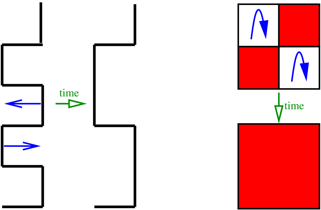
Figure 1: (Color online). Upper part: A flat surface in $d=2$ with a distortion (left) and a bubble of reversed spins (right). Lower part: The increase of $L(t)$ in $d=2$ when features such as distortions (left) or bubbles (right) are removed.

II.1 Relation between the relaxation of a feature and the exponent $z$

In order to have coarsening, features must be progressively removed nota1 , by flipping all their spins. Let us define $\tau_{l}$ as the typical time to complete this process for a feature of size $l$. Our strategy is to relate $\tau_{l}$ to the growth exponent $z$. In order to do that, let us notice that when, after a time $\tau_{l}$, features of size $l$ are removed, the typical scale of the system is increased by a quantity $\Delta l\propto l$, as shown in Fig. 1 (lower part). Assuming scaling, namely the presence of a single relevant lengthscale, the typical size $l$ of a feature at time $t$ must be of order $L(t)$. Therefore $dL(t)/dt\simeq\Delta l/\tau_{l}$. Let us anticipate what will be shown in the next Section, namely that $\tau_{l}\propto l^{\alpha}$, with $\alpha=2$. Therefore we have $dL(t)/dt\propto L(t)^{1-\alpha}$, and so $L(t)\propto t^{1/z}$ with

$$z=\alpha=2.$$ (6)

In the following we consider the behavior of $\tau_{l}$.

II.2 Relaxation time of a feature

We use the terminology of the case $d=2$, for simplicity, but the argument is general. Let us consider the relaxation of an initially (at time $t=0$) squared bubble, represented in Fig. 2. At zero temperature only spins with $n\leq 0$ can be flipped. Therefore, referring to the situation of the upper part of Fig. 2, the first move is necessarily the flip of one of the four spins in the corners of the square.

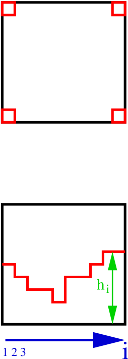
Figure 2: (Color online). Relaxation of a bubble in $d=2$. Upper: only the spins in the corner can be flipped initially. Lower: a typical configuration at a generic time.

These moves trigger a sequence of successive flips, producing the shrinking of the bubble. Let us suppose, in order to simplify the argument, that spins are flipped starting from the bottom of the box (actually the flipping of the spins proceeds on the average from each side, but this does not change our conclusions). Let us denote with $h_{i}$ ($i=1,2,\dots,l$) the height of the $i$-th column of the box at time $t$, as shown in Fig. 2. Due to the zero temperature constraints, while the first and last column, with $i=1$ and $i=l$, are always allowed to grow, due to the presence of the wall, all the other columns can do it only if at least one the nearest columns is higher. Moreover, a column cannot decrease its height if it is not higher than at least one of the neighborings. With these rules, columns evolve until, at $t=\tau_{l}$, all the spins in the box are flipped, the bubble disappears, and the process ends.

Since with this dynamics an exact evaluation of $\tau_{l}$ is not possible, in the following we consider a slightly modified kinetics for which a determination of $\tau_{l}$ is allowed; we will then argue, checking this hypothesis numerically, that the modification of the dynamics does not change significantly the behavior of $\tau_{l}$ and, in particular, the exponent $\alpha$. More precisely, we modify the original dynamics by introducing an additional constraint, namely $|h_{i+1}-h_{i}|\leq 1$. With this modification the problem can be mapped onto a diffusion equation for the variables $h_{i}$. This result, which applies to the case $d=3$ as well, is shown in Appendix I. For an interface described by a diffusion equation one has $\tau_{l}\propto l^{\alpha}$, with $\alpha=2$. We argue that the same result applies to the original dynamics as well. The reason is the following: due to all the constraints discussed above, the heights $h_{i}$ are not independent, the typical differences $|h_{i+1}-h_{i}|$ do not grow very large and, for large $l$, they are independent of $l$. This is confirmed by looking at a simulation of the bubble shrinking. For large $l$, since the differences $|h_{i+1}-h_{i}|$ are small as compared to the relevant scale $l$, we expect that the effect of the additional constraint does not change the exponent $\alpha$. This last statement is convincingly confirmed by the results of numerical simulations, shown in Fig. 3. This figure refers to the simulation of a squared (cubic in $d=3$) bubble, namely an Ising model on an $l^{2}$ ($l^{3}$ in $d=3$) squared lattice with (say) up spins on the boundary and an initial condition of down spins in the interior. Averaging over several ($10^{3}-10^{5}$, depending on $l$) realizations of the thermal history, for each value of $l$ we have computed $\tau_{l}$ as the time needed to revert the last spin. Fig. 3 shows that $\tau_{l}\propto l^{\alpha}$, with $\alpha=2$ is found with very good accuracy, regardless of dimensionality. This result confirms the validity of the hypothesis according to which the exponent $\alpha$ is the same ($\alpha=2$) in the original Ising dynamics and in the modified kinetics considered in Appendix I.

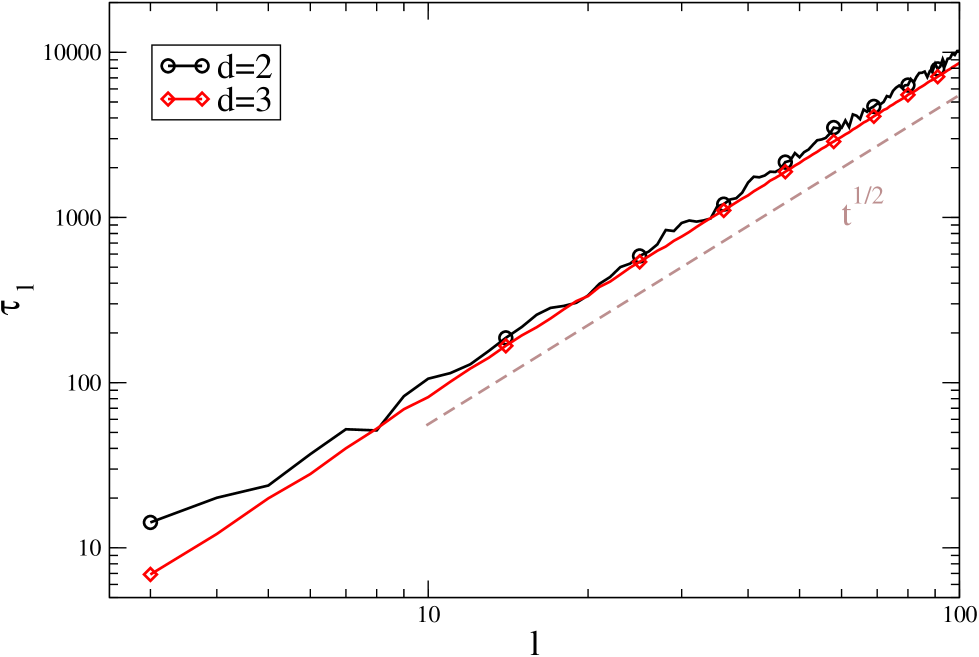
Figure 3: (Color online). The typical time $\tau_{l}$ needed to flip all the spins of a squared bubble of size $l$.

With this result Eq. (6) follows, namely $z=2$ in every dimension. The exponent $z$ is therefore the same as in quenches to finite temperatures. Assuming scaling, the size of domains $L(t)$ is related by $L(t)\propto\rho(t)^{-1}$ to the total density of interfaces present in the system. The exponent $z$ therefore gives informations on the number of interfaces, not on their geometry. In order to appreciate geometrical properties we will consider in the following other observables.

II.3 Densities of spins with a given degree of alignment.

Restricting again to the $d=2$ case for simplicity ( the extension to the case $d=3$ is straightforward and will be discussed in Appendix II). we introduce the density $\rho_{n}(l)$ of spins with a certain degree of alignment $n_{i}=n$ in a feature. In the following, we will only refer to interfacial spins: bulk spins with $n=4$, whose behavior is trivial, will never be considered. Initially, in the squared bubble interfacial spins are those on the flat boundaries or in the corners, with $n=2$ and $n=0$ respectively. During the evolution, as shown in the lower part of Fig. 2, all the possible values of $n$ can be generated. The set of $\rho_{n}(l)$ provides a geometric characterization of the interface. A representation of the typical geometry where a spin with a degree of alignment $n$ occurs when the bubble shrinks is drawn in Fig. 4

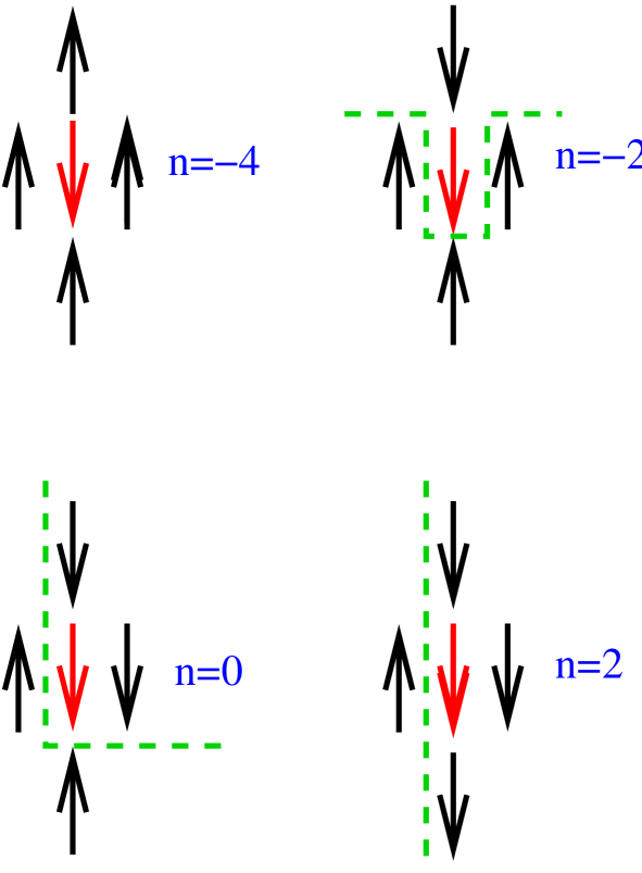
Figure 4: (Color online). Classification of interfacial spins in $d=2$. The central spin is classified according to the degree of alignment. The dashed line is the typical shape of the interface associated to each type of spin during the bubble shrinkage.

While columns are growing, a generic profile of $h_{i}$ is made of steps, namely spins with $n=0$, and flat parts with $n=2$, as shown in Fig. 2. A step on site $i$ can be randomly replaced by a flat part and the reverse is possible as well. As a consequence for sufficiently large values of $l$ a finite fraction, independent of $l$, of spins with $n=0$ and $n=2$ will be typically present. Simulations clearly show that these numbers, on average, do not depend on time (excluding, possibly, the initial and final stages of the process). According to this, the number of spins with $n=0$ or $n=2$ is constant and proportional to the length of the interface, namely to $l$. Normalizing with the total number of spins $l^{2}$, we obtain $\rho_{2}(l)\propto l^{-1}$ and $\rho_{0}(l)\propto l^{-1}$. The situation is very different for spins with $n=-2$ and $n=-4$. The former can only be produced when a last spin must be reversed in order to complete a row, an event happening, on average, every $l$ moves. When this occurs, a single spin (out of $l^{2}$) with $n=-2$ is generated. Looking at a generic time, therefore, the typical density of such spins is $\rho_{-2}(l)\propto l^{-3}$. Finally, spins with $n=-4$ are only obtained when the last spin of the box must be reversed. In a bubble of $l^{2}$ spins only one can be the last, and this happens once every $l^{2}$ moves. Hence $\rho_{-4}(l)\propto l^{-4}$. Again, scaling implies that we can identify $l$ and $L(t)$, leading to

$$\rho_{n}[L(t)]\propto L(t)^{-\beta_{n}},$$ (7)

with

$$\beta_{2}=\beta_{0}=1,$$ (8)

$$\beta_{-2}=3,$$ (9)

$$\beta_{-4}=4.$$ (10)

This argument can be extended to the case $d=3$ (see Appendix II). The results are

$$\beta_{4}=\beta_{2}=\beta_{0}=1,$$ (11)

$$\beta_{-2}=3,$$ (12)

$$\beta_{-4}=\beta_{-6}=4.$$ (13)

In the next Section we will compare these predictions with the outcome of numerical simulations, both in $d=2$ and $d=3$.

III Numerical simulations

III.1 Quenches to $T_{f}=0$.

We have simulated systems of $2000^{2}$ and $576^{3}$ spins in $d=2$ and $d=3$, respectively, on square (cubic) lattices. With these sizes, we have checked that finite size effects are not present in the range of times presented in the figures. The critical temperature of the model is $T_{c}\simeq 2.269$ and $T_{c}\simeq 4.512$ in $d=2$ and $d=3$ respectively (we set $J=1$). Time is measured in montecarlo steps (mcs). In Fig. 5 we show the results for $d=2$. Here we observe that a scaling regime, attested by the power law behavior of all the plotted quantities, sets in after a very short time $t_{sc}\simeq 4$ mcs. Best power law fits to the data (for $t\geq 10$) give $\beta_{2}=0.99\pm 0.02$, $\beta_{0}=1.03\pm 0.03$, $\beta_{-2}=2.99\pm 0.04$, $\beta_{-4}=4.05\pm 0.05$, and $z=1.99\pm 0.02$. All the exponents $\beta_{n}$ and $z$ are in excellent agreement with the determination made in the previous Section.

When scaling holds, according to Eqs. (2),(3) the equal time correlation function, behaves as

$$G_{ag}(r,t,t)=h(r/L(t)),$$ (14)

with $h$ obeying Porod law (4) in the case of sharp interfaces. In the case considered here, $G_{ag}(r,t,t)=G(r,t,t)$, since $G_{st}(r,t,t)\equiv 0$ at $T_{f}=0$. According to Eq. (14), when scaling holds curves of $G_{ag}(\vec{r},t,t)$ for different times should collapse when plotted against $r/L(t)$. This is observed in Fig. 14 (left part). Besides, the Porod law (4) is very neatly obeyed.

Figure 5: (Color online). Quench to $T_{f}=0$ in $d=2$. The densities $\rho_{n}[L(t)]$ are plotted against $L(t)=\rho(t)^{-1}$. In the inset $L(t)$ is plotted against time.

In Fig. (6) a plot analogous to that of Fig. 5 is made for $d=3$.

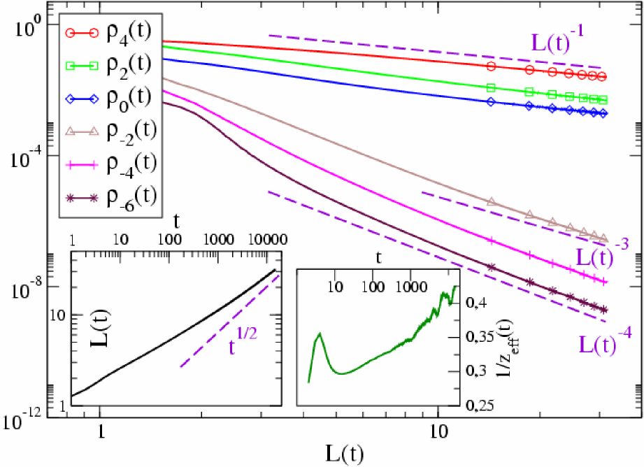
Figure 6: (Color online). Quench to $T_{f}=0$ in $d=3$. The densities $\rho_{n}[L(t)]$ are plotted against $L(t)=\rho(t)^{-1}$. In the insets $L(t)$ and $1/z_{eff}(t)$ are plotted against time.

After a time around 10 mcs a power-law behavior sets in for all the $\rho_{n}[L(t)]$. Fitting the curves with power laws we find a residual time dependence of the exponents $\beta_{n}$, since their value changes measuring them in different timewindows. This is particularly evident for $\beta_{-2}$. This indicates that preasymptotic corrections to scaling are not completely negligeable in the timedomain of our simulations. Best power-law fits for $t>10$ yield $\beta_{4}=0.97\pm 0.04$, $\beta_{2}=1.11\pm 0.06$, $\beta_{0}=1.03\pm 0.04$, $\beta_{-2}=3.3\pm 0.1$, $\beta_{-4}=3.8\pm 0.1$, and $\beta_{-6}=3.9\pm 0.1$. Taking into account the presence of preasymptotic corrections we regard these values as being consistent with the results of the previous Section. Regarding $L(t)$, instead, the data (in the inset) do not show a satisfactory power law. The curve is bending upwards on the double logarithmic plot and the exponent is not consistent with the expected value $z=2$. In order to clarify this point we have computed the effective exponent

$$\frac{1}{z_{eff}(t)}=\frac{d\ln L(t)}{d\ln t},$$ (15)

which is shown in the inset of Fig. 6. In an early stage, when scaling does not hold, this quantity grows exponentially as described by linear theories Cahn . Then, after reaching a minimum of order $0.3$, $1/z_{eff}(t)$ it keeps slowly, but steadily, increasing. Its value measured at the longest times is around $1/z_{eff}\simeq 0.43$. Actually, to the best of our knowledge, the expected exponent $z=2$ has never been reported. Previous simulations on much shorter timescales observed Amar89 an exponent of order $1/3$ and sometimes the very existence of dynamical scaling has been questioned. Notice that the value $1/3$ is comparable to the value $1/z_{eff}\simeq 0.3$ of the effective exponent around its minimum, a fact which may explain what reported in Amar89 . Our data are consistent with a possible asymptotic value $z=2$ although much larger simulation efforts would be needed for a definitive evidence. In any case, the data show that preasymptotic effects are quite relevant, and exclude that a well defined exponent can be measured, up to $t\simeq 2\cdot 10^{4}$ mcs (for longer times, not reported in the Figure, finite size effects are observed). A rough extrapolation suggests that times at least 10 times larger ($t\simeq 2\times 10^{5}$ mcs) are needed to observe $1/z_{eff}(t)\simeq 1/z\simeq 1/2$ (meaning a lattice size of order $(2\cdot 10^{3})^{3}$ in order to be finite size effects free).

III.2 Quenches to $T_{f}>0$.

When the quench is made to a finite final temperature all the constraints imposed by $T_{f}=0$ are removed. In the quench to $T_{f}=0$, as seen in Sec. III.1, spins with $n>0$ are present in the system, but they cannot be updated because this would increase the energy. When $T_{f}>0$ also these can be updated, although with a small probability for small $T_{f}$. For shallow quenches ($T\lesssim T_{c}$) the typical times $\tau_{n}(T_{f})=W(n_{i}[\sigma],T_{f})^{-1}$ associated to microscopic moves are small, and, in particular, much smaller then the timescales over which the non-equilibrium behavior of interfaces takes place. Therefore we expect that during phase-ordering an interface be in quasi equilibrium, namely it will have the same values of $\rho_{n}[L(t)]$ of an equilibrium interface nota4 of length $l=L(t)$ at the same temperature of the quench. In order to check this conjecture we have performed the following simulations: In $d=2$ we have prepared an Ising system with a spanning vertical interface in the middle and antiperiodic boundary conditions in the horizontal direction; subsequently, we let it evolve at a constant temperature $T$ and, during the evolution, we have measured the densities $\rho_{n}(l)$. These quantities are compared to the quantities $\rho_{n}[L(t)]$ measured in a quench to the final temperature $T_{f}=T$. In both the situations we have implemented a fast dynamics where spins with $n=4$ are not allowed to flip. This no bulk flip (NBF) dynamics has been frequently used in the literature Corberibis ; Corberi03 . Apart from its numerical efficiency, it has the advantage of isolating the aging behavior of the system. The reason is that since, as already pointed out in Sec. I, the stationary terms in Eq. (1) are produced by the flipping of the spins inside the domains, by preventing bulk moves one is left only with the dynamics of the interfaces which is responsible for the aging term of Eq. (1). On the other hand, it has shown Corberi03 also that the NBF rule does not change the properties of the aging terms in the large time domain. In the simulation of the single interface we use this no bulk flip (NBF) dynamics also as a tool to maintain a single interface in the system at all times. With the standard dynamics spins can be reversed in the bulk, creating additional interfaces that may interact with the original spanning interface. On the other hand, with NBF dynamics, the spanning interface remains unique and well defined at all times. In order to avoid the complications arising when comparing $\rho_{n}(l)$ with $\rho_{n}[L(t)]$ in the two kind of simulations, which would require the comparison of the size $l$ of the interface in the equilibrium simulation with the length $L(t)$ in the corresponding quenched system, in Fig.7 we have plotted the ratios between different $\rho_{n}$. Since these quantities do not depend on $l$ or on $L(t)$ respectively in the two cases, they can be directly compared. After a brief transient, the single interface (main figure) reaches the stationary state and the ratios between different $\rho_{n}$ take time-independent values. The same is true for the quenched system, shown in the inset. We find that the asymptotic value of the ratios is the same with good accuracy in the two systems. This confirms our claim that in a shallow quench the values of the densities $\rho_{n}[L(t)]$ are equal to the corresponding quantities $\rho_{n}(l)$ in an equilibrium interface of size $l$. Since the latter are finite and time-independent this implies that in a shallow quench $\rho_{n}[L(t)]\propto\rho(t)$. Therefore, instead of Eqs. (8-10), and Eqs. (11-13) one must have

$$\beta_{n}=1,$$ (16)

for every value of $n$. This is shown to be true in Fig. 8 for systems in $d=2,3$ quenched to $T_{f}=2$. Best power-law fits (for $t>10$) yield $\beta_{2}=1.00\pm 0.01$, $\beta_{0}=1.00\pm 0.01$, $\beta_{-2}=1.00\pm 0.01$, $\beta_{-4}=1.01\pm 0.1$, in $d=2$ and $\beta_{4}=1.00\pm 0.01$,$\beta_{2}=1.00\pm 0.01$,$\beta_{0}=1.00\pm 0.01$, $\beta_{-2}=1.00\pm 0.01$,$\beta_{-4}=1.01\pm 0.01$, $\beta_{2}=1.01\pm 0.02$, in $d=3$. Notice that the values of $\beta_{n}$ with $n<0$ are very different from the case with $T_{f}=0$ and can be used to distinguish the two kinds of dynamics. Regarding the value of the exponent $z$, the curvature driven mechanism implies $z=2$. Actually, this is found with very good accuracy in $d=3$ (we find $1/z=0.502\pm 0.04$ in the range $t\in[10^{2}-10^{4}]$). Instead, for $d=2$ one observes a slightly larger exponent, since $1/z$ is of order 0.48 in the region of the largest simulated times. We will comment later on this point.

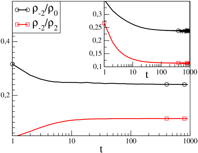
Figure 7: (Color online). The ratios between $\rho_{-2}(l)$, $\rho_{0}(l)$, and $\rho_{2}(l)$ are plotted against $t$ for an equilibrium interface in $d=2$ at $T=2$ (main) and in a quench to $T_{f}=2$ (inset). NBF dynamics is used in both cases.

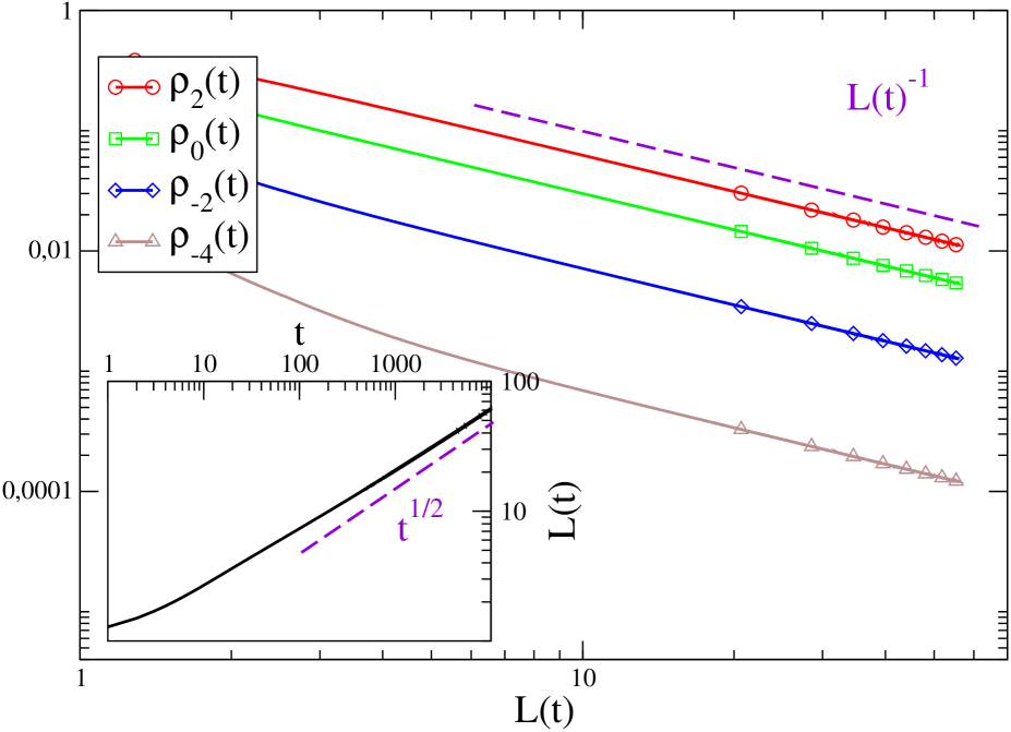
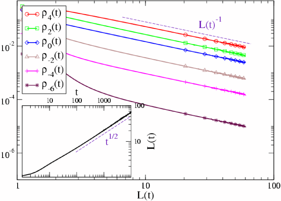
Figure 8: (Color online). Quench to $T_{f}=2$ (NBF), for $d=2$ (left) and $d=3$ (right). $\rho_{n}[L(t)]$ are plotted against $L(t)=\rho(t)^{-1}$. In the inset $L(t)$ is plotted against time.

Since the dynamics is different in shallow quenches or in quenches to $T_{f}=0$ we expect to see a crossover phenomenon at intermediate temperatures. Namely, for every $T_{f}>0$ a crossover time should exist separating an early stage where the dynamics is of the $T_{f}=0$ type, with $\beta_{n}$ given in Eqs. (8-10) for $d=2$ or in Eqs. (11-13) for $d=3$, from a late stage where the finite temperature scalings (16) set in. For a class of spins with a given degree of alignment $n$ the crossover between the early and the late kind of dynamics occurs when spins with the considered $n$ start to be created by means of activated moves. The crossover time, therefore, should be of order $\tau_{n}(T_{f})\simeq W(n,T_{f})^{-1}$, and is therefore different for spins with different $n$. At the crossover time $\tau_{n}(T_{f})$ a typical crossover length

$$L_{n}(T_{f})\simeq\tau_{n}(T_{f})^{1/z}=W(n,T_{f})^{-1/z}$$ (17)

is associated. In Figs. 9,10, the pattern of crossover described above can be observed. Here we see that, practically for all the $T_{f}$ considered, the behavior of the densities $\rho_{n}(t)$ is initially analogous to that of the $T_{f}=0$ case (Eqs. (8-10) or Eqs. (11-13) in $d=2$ or $d=3$ respectively). This regime lasts until $L(t)\simeq L_{n}(T_{f})$, where $\rho_{n}(t)$ start to behave as in shallow quenches (Eq. 16). For very small $T_{f}$, $L_{n}(T_{f})$ is outside the range of simulated times (this explains why, for instance, the curves with $T_{f}=0$ and $T_{f}=0.25$ can be hardly distinguished in $d=2$). Increasing $T_{f}$ gradually, $L_{n}(T_{f})$, whose values obtained from Eq. (17) are marked with vertical segments across the curves (when within the simulated times), become progressively smaller. One observes that the crossover phenomenon occurs at different times for spins with different $n$, and that the estimate (17) agrees reasonably well with what observed.

Figure 9: (Color online). $d=2$. $\rho_{-2}[L(t)]$ (left) and $\rho_{-4}[L(t)]$ (right) are plotted against $L(t)=\rho(t)^{-1}$ (NBF). Vertical segments across the curves represent the crossover lengths $L_{-2}(T_{f})$ and $L_{-4}(T_{f})$ of Eq. (17) (when reached in the simulation).

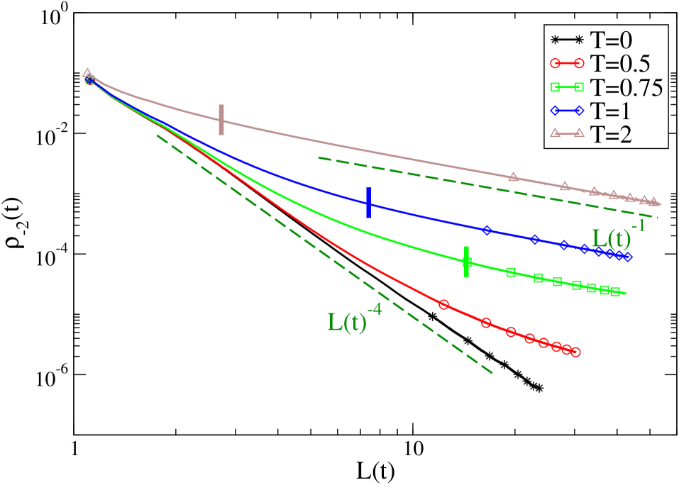
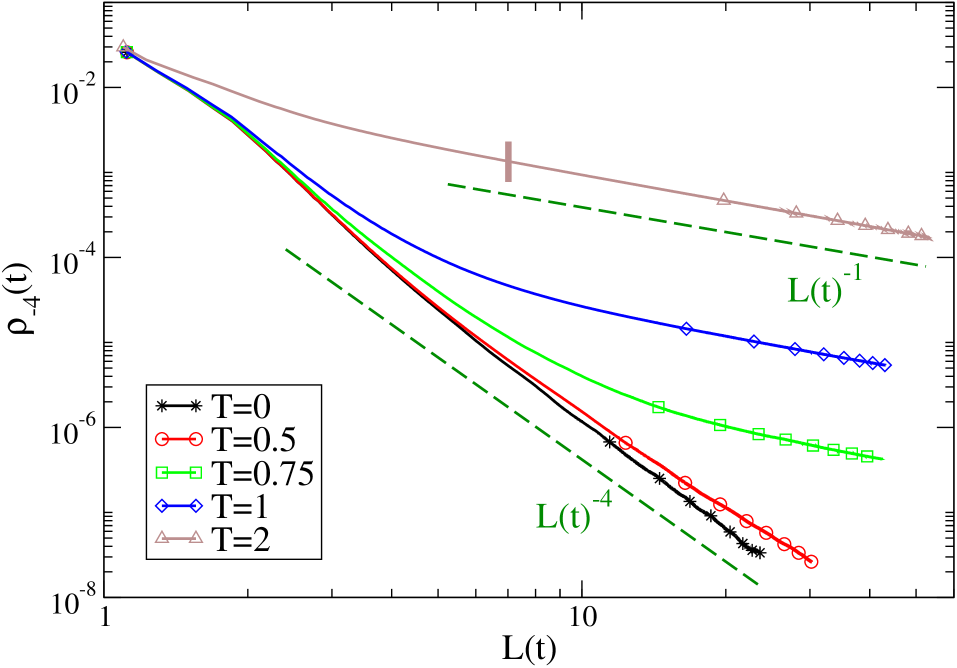
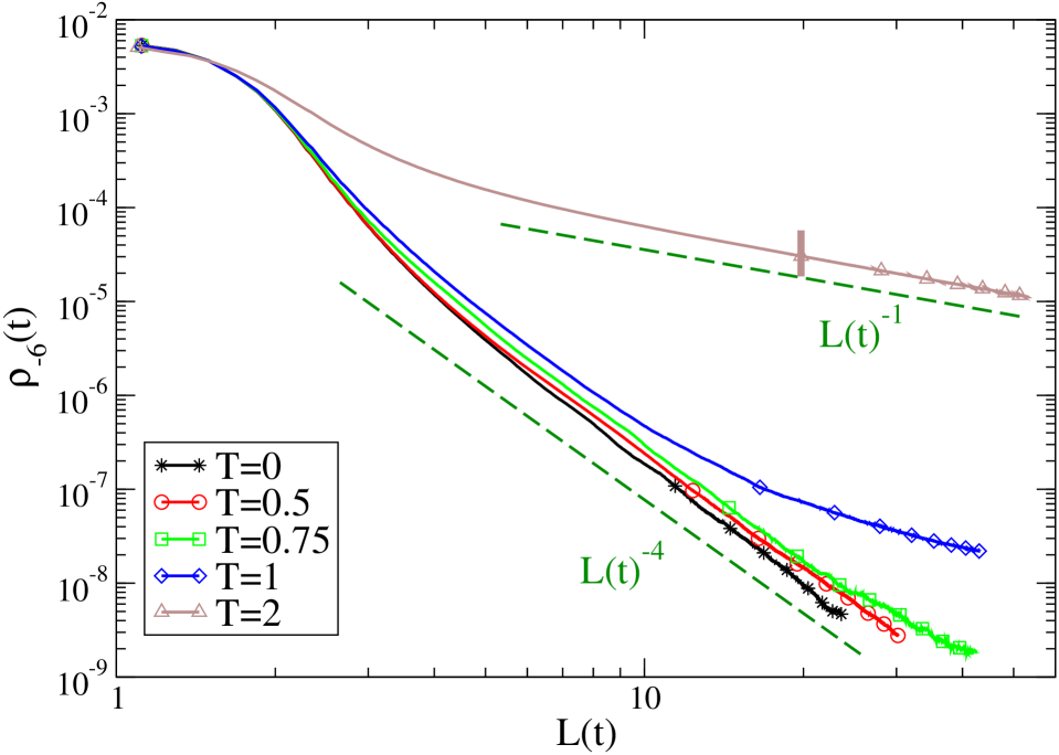
Figure 10: (Color online). $d=3$. $\rho_{-2}[L(t)]$, $\rho_{-4}[L(t)]$ and $\rho_{-6}[L(t)]$ are plotted against $L(t)=\rho(t)^{-1}$ (NBF). Vertical segments across the curves represent the crossover lengths $L_{-2}(T_{f})$, $L_{-4}(T_{f})$ and $L_{-6}(T_{f})$ of Eq. (17) (when reached in the simulation).

Let us now come back to the value of the exponent $1/z$ in $d=2$, which, as already observed regarding Fig. 8, has a value slightly smaller than the expected one $1/z=0.5$. In order to make more precise statements we have measured the effective exponent, which is shown in Fig. 11 for various temperatures. For $T=0$ the effective exponent initially rise to a maximum for the reasons already discussed for the case with $d=3$. Then it goes down to a minimum and, later, reaches the asymptotic value $0.5$ already at times of order $t\simeq 300$ mcs. As $T_{f}$ is increased the pattern is similar but the initial minimum is depressed and delayed so that for the largest temperatures considered $1/z_{eff}(t)$ has not yet reached the asymptotic value at the longest simulated times. Although the expected final value $1/z_{eff}=1/z=1/2$ is not in doubt, a rough determination of this exponent in a simulation may lead to a smaller value, as sometimes reported Manoy00 .

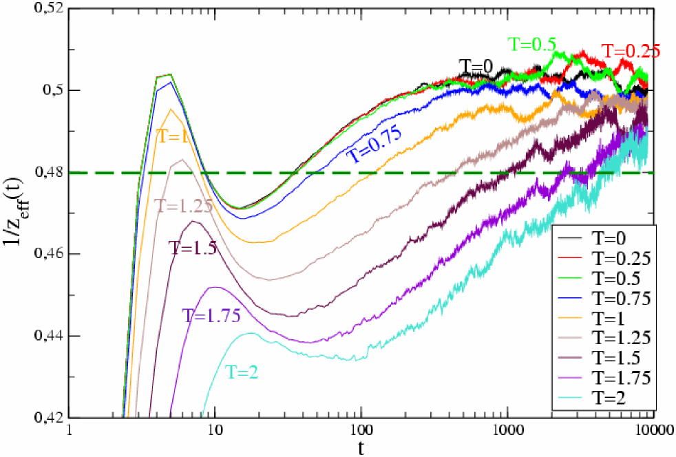
Figure 11: (Color online). The effective exponent $1/z_{eff}(t)$ for quenches in $d=2$ (NBF).

This behavior can be interpreted as due to the presence, beside $L(t)$, of another length, the roughness of the interfaces. Equilibrium interfaces are rough for $T>T_{R}$. The roughening temperature $T_{R}$ vanishes for $d=2$ while $0<T_{R}<T_{c}$ for $d=3$. An interface spanning a box of linear size $l$ in equilibrium at the temperature $T$ has a typical width $u_{l}(T)$ given by Barabasi

$$u_{l}(T)=\left\{\begin{array}[]{ll}a_{2}(T)\sqrt{l}\qquad$for$\qquad d=2\\ a_{3}(T)\qquad$for$\qquad d=3,T\leq T_{R}\\ a_{3}(T)\ln l\qquad$for$\qquad d=3,T>T_{R}.\end{array}\right.$$ (18)

In the phase-ordering kinetics it has been conjectured by Villain Abraham89 that the role of $l$ in Eq. (18) is played by $L(t)$. The non-equilibrium width $U(t,T_{f})$ should than behave as

$$U(t,T_{f})\propto\left\{\begin{array}[]{ll}a_{2}(T_{f})\sqrt{L(t)}\qquad$for$\qquad d=2\\ a_{3}(T_{f})\qquad$for$\qquad d=3,T_{f}\leq T_{R}\\ a_{3}(T_{f})\ln{L(t)}\qquad$for$\qquad d=3,T_{f}>T_{R}.\end{array}\right.$$ (19)

According to these expressions, in the large time limit $U(t,T_{f})$ can always be neglected with respect to $L(t)$. However, there can be an initial regime, for $t<t_{sc}$, where $U(t,T_{f})$ produces a correction to scaling. In this range of times we expect a (time dependent) effective exponent $z_{eff}(t)\neq 2$ to be observed. Given the behaviors (19), $t_{sc}$ may be sufficiently large to produce observable effects for $d=2$ while we expect it to be too small to significantly affect the scaling behavior for $d=3$. Actually, we have already observed (see Fig. 8) that, differently from $d=2$, in $d=3$ the effective exponent quickly converges to the value $z=2$ for quenches to $0<T_{f}<T_{c}$. According to our hypothesis, since $a(T_{f})$ is an increasing function of $T_{f}$, while $L(t)$ is roughly temperature independent, the convergence towards the asymptotic $z=2$ should be delayed increasing $T_{f}$: This is actually observed in Fig. 11. In order to check further the consistency of this hypothesis we have computed the temperature dependence of $a(l,T_{f})$. From a set of simulations of a single interface as those described above in this section we have extracted the equilibrium width of the interface as $u_{l}(T)=\langle\sqrt{\sum_{j=1}^{l}(1/l)[x_{j}(t)-l/2]^{2}}\rangle$, where $j$ is the vertical coordinate in the simulation box, $x_{j}(t)$ is horizontal coordinate of the interface position at a generic time $t$, and $\langle\cdots\rangle$ is an average over thermal realizations. Since in equilibrium $u_{l}(T)$ does not depend on time we have also averaged $u_{l}(T)$ over time in order to reduce the noise.

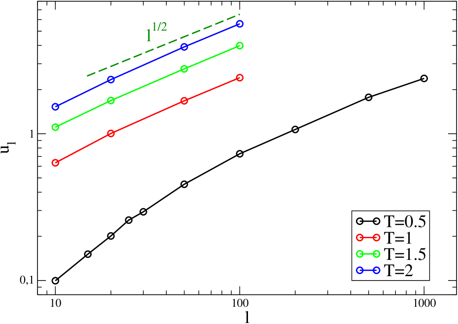
Figure 12: (Color online). $u_{l}(T)$ is plotted against $l$ for different temperatures.

Fig. 12 shows that the behavior (18) is obeyed for $l$ sufficiently large (the larger the lower is $T_{f}$). Extracting $a_{2}(T_{f})$ we find a linear relation

$$a_{2}(T_{f})=AT_{f},$$ (20)

where $A$ is a constant ($A\simeq 0.32$). We can evaluate $t_{sc}$ from the condition $L(t_{sc})=U(t_{sc},T_{f})$. In a quench from high temperature $L(t)$ start growing from an initial value $L(0)\simeq 1$. For low temperatures, since $a_{2}(T_{f})$ is very small, $L(0)$ is larger than $U(0,T_{f})$ and hence $U(t,T_{f})$ is negligible from the beginning. In this case scaling can set in very early, after the microscopic time $t^{*}\simeq 1$ necessary for the formation of domains of the equilibrium phases which is practically independent of $T_{f}$. For larger temperatures there is a transient during which $U(t,T_{f})$ cannot be neglected. Using Eqs. (19,20) one obtains $L(t_{sc})=A^{2}T_{f}^{2}$. Since $L(t)\sim t^{1/2}$ is roughly obeyed also for $t<t_{sc}$ (the effective exponent is always in the range $[0.45-0.5]$) one can estimate $t_{sc}\propto T^{4}$. In Fig. 13 we have plotted $L(t_{sc})$ for different values of $T_{f}$. This quantity have been obtained as follows: From the data of Fig. 11 we have estimated $t_{sc}$ as the time when $1/z_{eff}(t)$ reaches the value $0.48$ (clearly, we refer to the asymptotic increase of $1/z_{eff}(t)$, for $t>100$, not to the early maximum). Successively, from the numerical data for $L(t)$ we have extracted $L(t_{sc})$. The picture shows agreement with the prediction of our hypothesis, namely a constant value of $L(t_{sc})$ at low temperatures and a behavior $L(t_{sc})\sim T_{f}^{2}$ for larger temperatures.

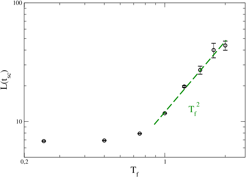
Figure 13: (Color online). $L(t_{sc})$ is plotted against $T_{f}$.

The interplay between $U(t,T_{f})$ and $L(t)$ can also be observed in the behavior of the equal time correlation function, which, when scaling holds, should behave as in Eq. (14), with $h$ obeying Porod law (4) in the case of sharp interfaces. However, as already discussed, the presence of $U(t,T_{f})$ introduces a correction to scaling in an early regime when $L(t)$ has not yet grown sufficiently larger than $U(t,T_{f})$. Moreover, due to roughness, interfaces are not sharp. Then, both scaling and the Porod law are expected to be violated for $r\lesssim U(t,T_{f})$, that is for $x=r/L(t)\lesssim x_{R}(t)=U(t,T_{f})/L(t)=a_{2}(T_{f})L^{-1/2}(t)$, namely in a range of $x$ that shrinks in time but that may be appreciable for large $T_{f}$. Actually this is observed in Fig. 14. While curves of $G_{ag}(r,t,t)$ for different times collapse when plotted against $r/L(t)$ for the quench to $T_{f}=0$, as discussed in Sec. III.1, and the Porod law is also verified, when the quench to $T_{f}>0$ is considered one observes significant scaling violations in the region of small $x$. In this regime, the curve definitely deviates from the linear Porod law. As time goes on, these violations become weaker and the curves seem to approach the same behavior as for $T_{f}=0$. For intermediate temperatures similar, but less pronounced, violations are also observed.

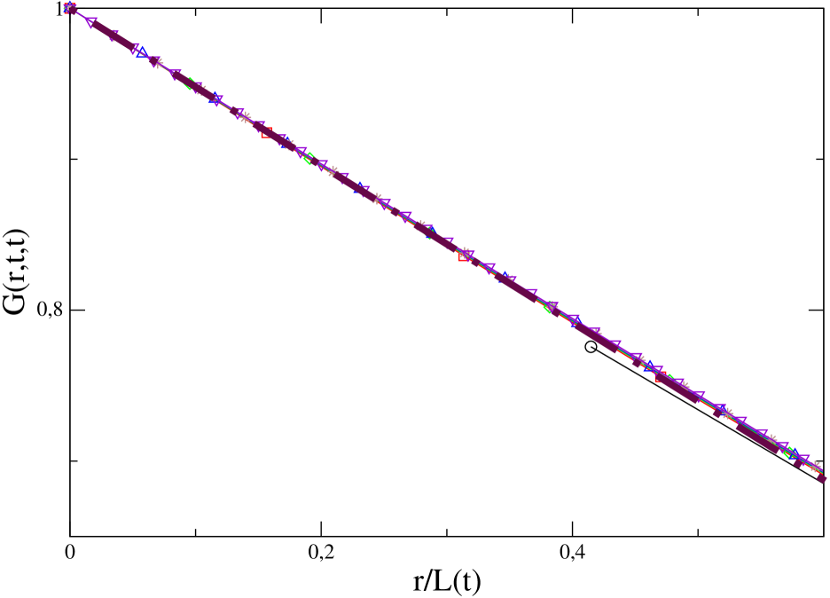
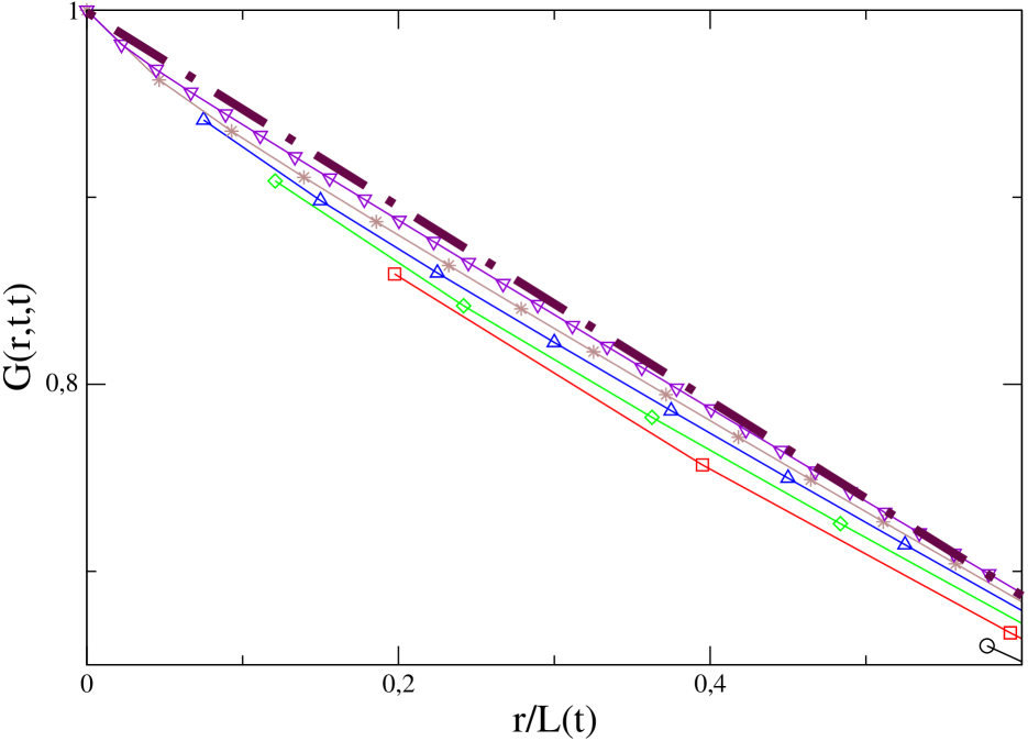
Figure 14: (Color online). $G(\vec{r},t,t)$ is plotted against $x=r/L(t)$ for a quench to $T=0$ (left) or $T=2$ (right). Different curves correspond to several times (the same in the two figures) between $t=10$ and $t=10^{4}$ (from bottom to top, for $T=2$). The dot-dashed line is the Porod law $y=1-ax$, where $a$ (the same in the two pictures) is obtained as the best fit of $G(\vec{r},t,t)$ at $T=0$. Points are joined by a piecewise continuous line as a guide for the eye (for clarity the first two points, the one in the origin and the following, are not joined).

IV Summary and conclusions

In this paper we have investigated the role of $T_{f}$ in the phase-ordering kinetics of the Ising model with single spin flip dynamics. At $T_{f}=0$ the dynamics is characterized by faceted interfaces and by the kinetic constraint of the impossibility of activated moves. At $T_{f}>0$ interfaces are curved and rough (for $T>T_{R}$ in $d=3$). We have shown that, while the exponent $z$ regulating the decay of the total density of interfacial spins is not changed by the different geometry of interfaces in quenches to $T_{f}=0$ or $T_{f}>0$, other quantities, such as the exponents $\beta_{n}$ describing the behavior of the densities of particular classes of spins do change. The existence of two different dynamical mechanisms induces a crossover pattern for finite $T_{f}$. Besides, in $d=2$ for $T_{f}>0$ the roughening length competes with $L(t)$ in an early stage, delaying the realization of dynamical scaling, as it is evidenced by the time dependence of the effective exponent $z_{eff}$ and by the breakdown of the Porod law at small $r/L(t)$.

This whole pattern of behaviors is due to equilibrium properties of the interfaces. Therefore we expect to observe similar behaviors for the Ising model with conserved dynamics.

APPENDIX I

We consider a generic profile of the $h_{i}$ and denote with $\{h\}$ this configuration. Let us introduce the probability $P(\{h\},t)$ of having such a configuration at time t, and the conditional probability $P(\{h^{\prime}\},t^{\prime}|\{h\},t)$ of having $\{h^{\prime}\}$ at time $t^{\prime}$ provided that the configuration $\{h\}$ was found at $t<t^{\prime}$. One has

$$\langle h_{i}(t+\Delta t)-h_{i}(t)\rangle=\sum_{\{h\},\{h^{\prime}\}}(h^{\prime}_{i}-h_{i})P(\{h^{\prime}\},t+\Delta t|\{h\},t)P(\{h\},t).$$ (21)

From the master equation, the conditional probability can be written as Lippiello05

$$P(\{h^{\prime}\},t+\Delta t|\{h\},t)=\left[1-\Delta t\sum_{j}\sum_{h^{\prime\prime}_{j}\neq h_{j}}w(h_{j}\to h_{j}^{\prime\prime})\right]\delta_{\{h^{\prime}\},\{h\}}+\Delta t\sum_{j}\sum_{h^{\prime\prime}_{j}\neq h^{\prime}_{j}}w(h_{j}^{\prime\prime}\to h_{j}^{\prime})\delta_{\{h^{\prime\prime}\},\{h\}}+{\cal O}(\Delta t^{2})$$ (22)

where we have introduced the transition rate $w(h_{j}\to h_{j}^{\prime})$ for moving the height $h_{j}$ of the $j$-th column to $h_{j}^{\prime}$ and $\delta_{\{h^{\prime\prime}\},\{h\}}$ is the Kronecker function between configurations $\{h^{\prime\prime}\}$ and $\{h\}$. We have assumed that the $w$ are single spin flip transition rates and hence transitions between configurations can be obtained by summing over $j$. Apart from this, the $w$ are still generic (not necessary those of the zero temperature Ising model) at this stage. Inserting Eq. (22) into Eq. (21), due to the term $(h^{\prime}_{i}-h_{i})$ only contributions with $\{h^{\prime}\}\neq\{h\}$ and $j=i$ survive, and one has

$$\langle h_{i}(t+\Delta t)-h_{i}(t)\rangle=\Delta t\sum_{\{h\},\{h^{\prime}\}\neq\{h\}}(h^{\prime}_{i}-h_{i})P(\{h\},t)w(h_{i}\to h_{i}^{\prime}).$$ (23)

Since in an elementary move $h_{i}\to h_{i}\pm 1$ is only allowed, introducing $m=\pm 1$ the last Equation reads

$$\langle h_{i}(t+\Delta t)-h_{i}(t)\rangle=\Delta t\sum_{\{h\}}\sum_{m}mw(h_{i}\to h_{i}+m)P(\{h\},t).$$ (24)

Taking the continuum limit $\Delta t\to 0$ yields

$$\frac{d\langle h_{i}(t)\rangle}{dt}=\sum_{\{h\}}\sum_{m}mw(h_{i}\to h_{i}+m)P(\{h\},t).$$ (25)

This equation has been obtained without any approximation. We now have to specify the form of the $w(h_{i}\to h_{i}+m)$ in order to reproduces the original rules of the zero temperature Ising model. However, in order to have a tractable model, we consider transition rates which correspond to the Ising model with the additional constraint

$$|h_{i+1}(t)-h_{i}(t)|\leq 1\quad\forall i,$$ (26)

as discussed in Sec. II.2. Starting with the case $d=2$, we define them as

$$w(h_{i}\to h_{i}+m)=\frac{m}{2}\nabla^{2}h_{i}+F_{i}^{(m)}(\{h\}),$$ (27)

where $\nabla^{2}h_{i}=h_{i-1}+h_{i+1}-2h_{i}$ is the discrete Laplacian in one dimension, and

$$F_{i}^{(m)}(\{h\})=\frac{1}{2}|\nabla^{2}h_{i}|\delta_{m\,sign\left(\nabla^{2}h_{i}\right),\,-1}.$$ (28)

In order to see this let us notice first that if the configuration $\{h\}$ satisfies the condition (26), with the transition rates (27) that constraint will never be violated by the later evolution. In fact, let us focus on site $i$ and suppose that the transition $h_{i}\to h_{i}+1$ is going to be attempted. This transition would violate Eq. (26) if $h_{i+1}=h_{i}-1$. In this case, however, it easy to check that for every $h_{i-1}$ consistent with the condition (26) it is $w(h_{i}\to h_{i}+1)=0$. The same argument can be repeated for every configuration. Having proved that  (26) is fulfilled by the transition rates (27) we can restrict ourselves to consider the only cases allowed, namely those with $\nabla^{2}h_{i}=0,\pm 1,\pm 2$. When $\nabla^{2}h_{i}=0$ the only configuration where the move $h_{i}\to h_{i}\pm 1$ could be attempted without violating the constraint (26) is that with $h_{i-1}=h_{i}=h_{i+1}$. In this case, in the original Ising model the move is forbidden, which agrees with Eq. (27) giving $w(h_{i}\to h_{i}+m)=0$ in this case. Coming to the cases with $\nabla^{2}h_{i}=\pm 1$ (which are realized, for instance, when $h_{i+1}=h_{i}=h_{i-1}\mp 1$), in the original Ising model moves with $m\,\,sign\left(\nabla^{2}h_{i}\right)<0$ are energetically forbidden, while those with $m\,\,sign\left(\nabla^{2}h_{i}\right)>0$ occur with a probability $1/2$, using Glauber transition rates. This agrees with Eq. (27). Analogously, when $\nabla^{2}h_{i}=\pm 2$ (when, for instance, $h_{i+1}=h_{i-1}$ and $h_{i}=h_{i+1}\mp 1$), in the original Ising model moves with $m\,\,sign\left(\nabla^{2}h_{i}\right)<0$ are forbidden, while those with $m\,\,sign\left(\nabla^{2}h_{i}\right)>0$ lower the energy and occur with a probability $1$, providing again agreement with Eq. (27).

Let us now insert the transition rates (27) into the evolution Equation (25), obtaining

$$\frac{d\langle h_{i}(t)\rangle}{dt}=\sum_{\{h\}}\sum_{m}\frac{m^{2}}{2}\nabla^{2}h_{i}P(\{h\},t)+\sum_{\{h\}}\sum_{m}mF_{i}^{(m)}(\{h\})P(\{h\},t).$$ (29)

Performing the sum over $m$ one has

$$\frac{d\langle h_{i}(t)\rangle}{dt}=\langle\nabla^{2}h_{i}\rangle+\langle F^{\pm}_{i}\rangle$$ (30)

where $F_{i}^{\pm}(\{h\})=F_{i}^{(1)}(\{h\})-F_{i}^{(-1)}(\{h\})$. Let us now consider the last term on the r.h.s. of Eq (30). We want to show that it can be neglected. We will show it separately, for all the possible values of $\nabla^{2}h_{i}$, namely $\nabla^{2}h_{i}=0,\pm 1,\pm 2$. For $\nabla^{2}h_{i}=0$, from Eq. (28), it is $F_{i}^{\pm}(\{h\})\equiv 0$. Let us consider now the contributions with $\nabla^{2}h_{i}=\pm 1$. This situation corresponds to spins with $n=0$, or steps in the terminology of Sec. II.3. These that can be flipped from $\sigma=1$ to $\sigma=-1$ and back without energy costs. Therefore the two values of the spin in this case occur with equal probability (i.e. 1/2) and, as $\nabla^{2}h_{i}$ changes its sign when the spin is reversed the contributions $\nabla^{2}h_{i}=\pm 1$ cancel in $\langle F^{\pm}_{i}\rangle$. The case $\nabla^{2}h_{i}=-2$ can never be realized in the kinetics because it would require a move with energy increase. Therefore, the terms with $\nabla^{2}h_{i}=0,\pm 1,-2$ do not contribute to the r.h.s. of Eq. (30). This is no longer true for $\nabla^{2}h_{i}=2$. This term corresponds, in the language of Sec. II.3, to a spin with $n=-2$ which, as explained in Sec. II.3, are created only when the last spin has to be reversed to complete a row. On average this happens once every $l$ moves. Therefore, although the contributions with $\nabla^{2}h_{i}=2$ do not strictly vanish, they provide a contribution $\langle F^{\pm}_{i}\rangle\propto 1/l$, which can be neglected in the large-$l$ limit. Then we arrive at the diffusion equation

$$\frac{d\langle h_{i}(t)\rangle}{dt}=\langle\nabla^{2}h_{i}\rangle$$ (31)

Let us turn now to the case $d=3$. Similarly to the case $d=2$, it is easy to check that the transition rates

$$w(h_{i}\to h_{i}+m)=\frac{m}{4}\nabla^{2}h_{i}+F_{i}^{(m)}(\{h\}),$$ (32)

with the following form of $F_{i}^{(m)}(\{h\})$

$$F_{i}^{(m)}(\{h\})=\frac{1}{4}|\nabla^{2}h_{i}|\delta_{m\,sign\left(\nabla^{2}h_{i}\right),\,-1}+f_{i}(\{h\})\delta_{m\,sign\left(\nabla^{2}h_{i}\right),\,1},$$ (33)

where $\nabla^{2}h_{i}$ is the discretized laplacian in $d=3$ and with the values of $f_{i}(\{h\})$ given in table 1, satisfy the constraint (26) and reproduce the Glauber transition rates of the original Ising model at $T=0$. Proceeding as for $d=2$ one arrives at

$$\frac{d\langle h_{i}(t)\rangle}{dt}=\frac{1}{2}\langle\nabla^{2}h_{i}\rangle+\langle F^{\pm}_{i}\rangle,$$ (34)

By reasoning as in $d=2$, one concludes that only sites with $|\nabla^{2}h_{i}|=1,2,3,4$, corresponding to spins with $E_{i}\neq 0$ contribute to $\langle F^{\pm}_{i}\rangle$, but these can be neglected for large $l$. Hence one arrives also in this case to a diffusion equation

$$\frac{d\langle h_{i}(t)\rangle}{dt}=\frac{1}{2}\langle\nabla^{2}h_{i}\rangle.$$ (35)

$\mid\nabla^{2}h_{i}\mid$	$f_{i}(\{h\})$
0	0
1	-1/4
2	$\left\{\begin{array}[]{ll}-1/2\quad for\quad\nabla^{2}_{x}=0\,\,or\,\,\nabla^{2}_{y}=0\\ 0\quad\quad\quad else\\ \end{array}\right.$
3	1/4
4	0

Table 1: The values of the function $f_{i}(\{h\})$. $\nabla^{2}_{x}$ ($\nabla^{2}_{y}$) is the discrete second derivative along $x$ ($y$).

APPENDIX II

Let us consider the shrinkage of a cubic bubble of linear size $l$, and extend the argument developed in Sec. II.3 to the case $d=3$. The interfacial spins can be classified according to $n$, as shown in Fig. 15.

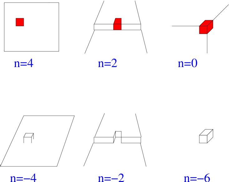
Figure 15: (Color online). Classification of interfacial spins.

Suppose again that the interface grows from the bottom of the bubble. Let us define $h_{i}$ as the height of the $i-$th column, with $i=1,...,l^{2}$ running on the two-dimensional lattice. While columns are growing, the profile of $h_{i}$ is made of flat parts (spins with $n=4$), edges (spins with n=2) and corners (spins with $n=0$). We make again the hypothesis that the probability of their occurrence is finite and constant. By reasoning analogously to the $d=2$ case, since these spins belong to the growing surface, their number is proportional to $l^{2}$. Hence $\rho_{4}(l)\propto\rho_{2}(l)\propto\rho_{0}(l)\propto l^{-1}$. Let us imagine to reverse the spins from the bottom, level by level. A spin with $n=-4$ is only produced when the last spin of a certain level has to be reversed. All the $l$ levels are completed in a time $\tau_{l}\propto l^{2}$, so that there is a number proportional to $l^{-1}$ of spins with $n=-4$ in a unit time. This implies $\rho_{-4}(l)\propto l^{-4}$. Spins with $n=-2$ are generated analogously to the spins with $n=-2$ in $d=2$, namely when the last spin must be reversed in order to complete a row. $l^{2}$ rows must be completed in a time $\tau\propto l^{2}$ in order to reverse all the spins of the bubble. Therefore there are $l^{0}$ spins with $n=-2$ in a unit time. In conclusion $\rho_{-2}(l)\propto l^{-3}$. Finally, spins with $n=-6$ are only formed when a growing column reaches the top of the bubble, with the condition that all the nearest column have already reached the top. Due to the kinetic constraints, these neighboring column must themselves have at least one nearest column of equal or higher eight. One can iterate this argument until a border is reached. Since the border is a distance of order $l$ away, one concludes that every $l$ spins only one can have $n=-6$. Therefore a number proportional to $l$ of spins are generated when the columns reach the top, and this event happens once every $\tau_{l}\propto l^{2}$ moves. Then $\rho_{-6}(l)\propto l^{-4}$. Assuming scaling, and identifying $l$ with $L(t)$ in the phase-ordering kinetics one arrives at Eqs. (11-13).

References

- (1) For a review see A.J. Bray, Adv.Phys. 43, 357 (1994).
- (2) H. Furukawa, J.Stat.Soc.Jpn. 58, 216 (1989); Phys.Rev. B 40, 2341 (1989).
- (3) D.S. Fisher and D.A. Huse, Phys. Rev. B 38, 373 (1988);
- (4) N. Mason, A.N. Pargellis and B. Yurke, Phys. Rev. Lett. 70, 190 (1993); F. Liu and G.F. Mazenko, Phys. Rev. B 44, 9185 (1991).
- (5) P.C. Hohenberg and B.I. Halperin, Rev. Mod. Phys. 49, 435 (1977).
- (6) G.F. Mazenko and O.T. Valls Phys. Rev. B 26, 389 (1982); G.F. Mazenko, O.T. Valls, and F.C. Zhang, Phys. Rev. B 31, 4453 (1985); Phys. Rev. B 32, 5807 (1985); Z.W. Lai, G.F. Mazenko, and O.T. Valls, Phys. Rev. B 37, 9481 (1988); C. Roland and M. Grant, Phys. Rev. B 39, 11971 (1989); Phys. Rev. Lett. 60, 2657 (1988).
- (7) A.J. Bray, Phys. Rev. Lett. 62, 2841 (1989); Phys. Rev. B 41, 6724 (1990).
- (8) Limited to the case , some exact result have been derived in: J.J. Arenzon, A.J. Bray, L.F. Cugliandolo and A. Sicilia, Phys. Rev. Lett. 98, 145701 (2007); A. Sicilia, J.J. Arenzon, A.J. Bray, L.F. Cugliandolo, Phys. Rev. E 76, 061116 (2007).
- (9) S.M. Allen and J.W. Cahn, Acta Metall. 27, 1085 (1979); I.M. Lifshitz, Zh. Eksp. Teor. Fiz. 42, 1354 (1962) [Sov. Phys. - JETP 15, 939 (1962).
- (10) G. Brown and P.A. Rikvold, Phys. Rev. E 65, 036137 (2002).
- (11) J.G. Amar and F. Family, Bull. Am. Phys. Soc. 34, 491 (1989); J.D. Shore, M. Holzer and J.P. Sethna, Phys. Rev. B 46, 11376 (1992).
- (12) The scaling approach we develop here recalls that of Ref. Bray98 , where the exponent is determined by evaluating the relaxation time of a distorted interface, but in the framework of continuum theories.
- (13) J.W. Cahn, Acta Metall. 9, 795 (1961); Acta Metall. 10, 179 (1962); Acta Metall. 14, 1685 (1966); Trans. Metall. Sec. AIME 242, 166.
- (14) By equilibrium interface we mean the stationary state of an interface in an Ising system with antiperiodic boundary condition in one direction.
- (15) R. Burioni, D. Cassi, F. Corberi, and A. Vezzani, Phys. Rev. E 75, 011113 (2007); F. Corberi, E. Lippiello, and M. Zannetti, Phys. Rev. E 74, 041106 (2006); R. Burioni, D. Cassi, F. Corberi, and A. Vezzani, Phys. Rev. Lett. 96, 235701 (2006); F. Corberi, E. Lippiello and M. Zannetti, Phys.Rev. E 68, 046131 (2003); F. Corberi, E. Lippiello, and M. Zannetti, Phys. Rev. E 63, 061506 (2001); F. Corberi, E. Lippiello, M. Zannetti, Eur. Phys. J. B 24 (2001), 359.
- (16) F. Corberi, E. Lippiello and M. Zannetti, Phys. Rev. E 72, 056103 (2005).
- (17) G. Manoy and P. Ray, Phys. Rev. E 62, 7755 (2000); E. Lippiello, F. Corberi, and M. Zannetti, Phys.Rev.E 74, 041113 (2006).
- (18) A.-L. Barabási and H. E. Stanley, Fractal Concepts in Surface Growth, (Cambridge University Press, Cambridge, 1995).
- (19) The argument is quoted in D. B. Abraham and P. J. Upton, Phys. Rev. B 39, 736 (1989).
- (20) E. Lippiello, F. Corberi, and M. Zannetti, Phys.Rev.E 71, 036104 (2005).
- (21) A.J. Bray, Phys. Rev. E 58, 1508 (1998).