Fully adaptive multiresolution schemes for strongly degenerate parabolic equations with discontinuous flux

Abstract.

A fully adaptive finite volume multiresolution scheme for one-dimensional strongly degenerate parabolic equations with discontinuous flux is presented. The numerical scheme is based on a finite volume discretization using the approximation of Engquist-Osher for the flux and explicit time stepping. An adaptive multiresolution scheme with cell averages is then used to speed up CPU time and memory requirements. A particular feature of our scheme is the storage of the multiresolution representation of the solution in a dynamic graded tree, for sake of data compression and to facilitate navigation. Applications to traffic flow with driver reaction and a clarifier-thickener model illustrate the efficiency of this method.

1. Introduction

1.1. Scope of the paper

High resolution finite volume schemes for the approximation of discontinuous solutions to conservation laws are of at least second-order accuracy in regions where the solution is smooth and resolve discontinuities sharply and without spurious oscillations. Methods of this type include the schemes described in [1, 2, 3, 4, 5, 6]. In standard situations, the solution $u(x,t)$ of a conservation law

(1.1) $$u_{t}+f(u)_{x}=0,\quad(x,t)\in Q_{T}:=\Omega\times[0,T],\quad\Omega\subseteq\mathbb{R}$$

exhibits strong variations (shocks) in small regions but behaves smoothly on the major portion of the computational domain. The multiresolution technique adaptively concentrates computational effort associated with a high resolution scheme on the regions of strong variation. It goes back to Harten [7] for hyperbolic equations and was used by Bihari and Harten [8] and Roussel et al. [9] for parabolic equations. Important contributions to the analysis of multiresolution methods for conservation laws include [10, 11, 12].

In this paper, we present a fully adaptive multiresolution scheme and corresponding numerical experiments for strongly degenerate parabolic equations with discontinuous flux. Specifically, we consider equations of the type

(1.2) $$u_{t}+f\bigl{(}\boldsymbol{\gamma}(x),u\bigr{)}_{x}=\bigl{(}\gamma_{1}(x)A(u)_{x}\bigr{)}_{x}\quad\text{for $x\in\Pi_{T}:=\mathbb{R}\times(0,T]$,}$$

where we assume that for each $x$, the function $f(\boldsymbol{\gamma}(x),\cdot):\mathbb{R}\to\mathbb{R}$ is piecewise smooth and Lipschitz continuous, and that $\boldsymbol{\gamma}(x)$ is a vector of scalar parameters that are discontinuous at most at a finite number of points. On the other hand, we assume that the integrated diffusion function $A(\cdot)$ is Lipschitz continuous and piecewise smooth with $A(v)\geqslant A(u)$ for $v>u$. We admit intervals $[\alpha,\beta]$ with $A(u)=\mathrm{const.}$ for all $u\in[\alpha,\beta]$, such that (1.2) degenerates into the first-order equation

(1.3) $$u_{t}+f\bigl{(}\boldsymbol{\gamma}(x),u\bigr{)}_{x}=0$$

wherever $u\in[\alpha,\beta]$. If degeneracy occurs on $u$-intervals of positive length (and not only at isolated points), (1.2) is called strongly degenerate. Clearly, solutions of (1.2) are in general discontinuous, and need to be characterized as weak solutions along with an entropy condition. Applications of (1.2) with constant parameters include models of sedimentation-consolidation processes of particulate suspensions [13, 14], two-phase flow in porous media [15], and traffic flow with driver reaction [16, 17]. Applications with a discontinuous parameter vector $\boldsymbol{\gamma}(x)$ include models of traffic flow on highways with discontinuous road surface conditions [16, 18], and a model of clarifier-thickener units used in engineering applications for the continuous solid-liquid separation of suspensions [19, 20]. In the latter application, the function $A(u)$ models sediment compressibility; the special case $A\equiv 0$, in which we fall back to (1.3), corresponds to a so-called ideal suspension of rigid spherical particles forming incompressible sediments. See [20] for further applications.

The novelty of the present paper is that we apply an adaptive multiresolution method to one-dimensional initial-value problems for (1.2). This equation is discretized in space by a first-order conservative finite volume scheme using the Engquist-Osher approximation, for which convergence results for our class of problems are available [16, 19, 20, 21, 22]. For time discretization an explicit Euler scheme is used. The multiresolution representation of the solution allows to introduce a locally refined mesh by thresholding of the wavelet coefficients while controlling the error of the approximation. This allows us to reduce the number of costly flux evaluations with respect to the finite volume scheme on a regular fine grid. Hence, a gain in CPU time can be obtained. Furthermore, the data are efficiently represented in a dynamic graded tree data structure, which also leads to memory compression.

1.2. Multiresolution schemes

In the following, we briefly outline the underlying ideas of multiresolution schemes for conservation laws and parabolic equations. The starting point is a conservative high-resolution finite volume discretization on a uniform mesh of (1.1) or (1.3). A multiresolution analysis of the solution with subsequent thresholding of the coefficients allows an approximation with less coefficients within a given tolerance. This allows us to reduce the number of costly flux evaluations required by the high-resolution scheme, which results in a gain of efficiency. For this purpose, either point values or cell averages of the numerical solution are defined on a hierarchical sequence of nested dyadic grids. Applying a multiresolution analysis to the solution, which can be efficiently done using the fast wavelet transform, we can construct a truncated representation by simple thresholding of the obtained coefficients. This procedure yields an efficient representation of the solution on a locally refined grid while controlling the error of the approximation.

The principle of multiresolution data representation consists in considering grid averages of the data at different resolutions from the finest to the coarsest grid, and in encoding the differences between two grids. Finally, one retains only the grid averages on the coarsest grid and the set of errors (or details) for predicting the grid averages of each resolution level in this hierarchy from those of the next coarsest one. In regions where the solution is sufficiently smooth, the multiresolution coefficients are small and can hence be neglected. Thus, data can be compressed by a thresholding or truncation operation, i.e. by setting to zero those components of the representation whose multiresolution coefficients (also called wavelet coefficients or details) are in absolute value smaller than a prescribed tolerance. Thresholding allows to control the so-called perturbation error thanks to norm equivalences. The representation of the solution in physical space corresponds to a locally refined grid.

The multiresolution analysis of the numerical solution automatically detects discontinuities, since a wavelet coefficient takes into account the regularity of a function in each position and on each scale. In [7, 23, 24] Harten explored this idea and introduced multiresolution schemes for efficiently solving hyperbolic conservations laws. Using the multiresolution representation of the solution, he devised a sensor to decide at which positions of a fine mesh the flux should be exactly evaluated, and where otherwise it can be obtained more cheaply by interpolation of pre-calculated fluxes on coarser scales. Still in the context of hyperbolic conservation laws and preserving flux evaluations for all fine grid positions, Bihari and Harten [8] developed a second-order adaptive switch for flux evaluations, keeping an essentially non-oscillatory (ENO) scheme where multiresolution coefficients were larger than a given tolerance, and otherwise using interpolation. In [25], Daubechies wavelets were used as a grid refinement strategy associated with finite difference stencils on an irregular grid for solving hyperbolic equations. Centered finite differences are used in [26] for approximating space derivatives on sparse point approximations (SPR) obtained by interpolating wavelet transforms. An SPR-based multiresolution WENO scheme is presented in [27]. For parabolic PDEs a finite volume method with dynamical adaptation strategy to advance the grid was developed in [9].

An alternative adaption strategy could be based on local a posteriori error estimates by means of residual error computation. Results of a posteriori error estimates have been reported in the literature for elliptic problems (see [28]), parabolic problems (see [29], [30]) and hyperbolic problems (see [31], [32] and the references therein), but there is not known results for strongly degenerate parabolic problems. In this sense, to compute local error estimator is not easy to be realized in practice, and we prefer to concentrate our effort in the strategy based on multiscale technique. The multiresolution strategy proposed herein for strongly degenerate parabolic equations with a discontinuous flux produces a gain in computational time and in memory. The solution is efficiently represented using a graded tree data structure and the costly fluxes are computed on the locally refined grid only. The computational efficiency of the multiresolution method is related to the data compression rate, that is, to the amount of significant information preserved after thresholding in comparison with the number of grid points of the finest mesh. Thus, efficiency is measured in terms of the compression rate and CPU time.

Finally, although we limit our treatment to one space dimension, the multiresolution scheme can be extended to higher dimensional problems in different ways. One possibility is to use higher dimensional wavelet transforms constructed by a tensor product approach, and through interpolations of the numerical divergence in the sense of cell averages from coarser to finer levels, the method of predicting values hierarchically can be extended as done in [33]. Another possibility is to explore the splitting capability of the divergence by directions as in [34]. Fully three-dimensional computations of flame instabilities are presented in [35].

1.3. Strongly degenerate parabolic equations and conservation laws with discontinuous flux

Equation (1.2) combines two independent non-standard ingredients of conservation laws: the strongly degenerate diffusion term $A(u)_{xx}$, and the flux $f(\boldsymbol{\gamma}(x),u)$ that depends discontinuously on the spatial position $x$. We briefly review some recent results for equations that include either ingredient.

The basic difficulty associated with degenerate parabolic equations of the type

(1.4) $$u_{t}+f(u)_{x} =A(u)_{xx},\quad x\in\Omega\subseteq\mathbb{R},\quad t\in(0,T]$$

is that their solutions need to be defined as weak, in general discontinuous solutions along with an entropy condition to select the physically relevant weak solution. In [14] the existence of $BV$ entropy weak solutions to an initial-boundary value problem for (1.4) in the sense of Kružkov [36] and Vol’pert and Hudjaev [37, 38] is shown via the vanishing viscosity method, while their uniqueness is shown by a technique due to Carrillo [39]. The well-posedness of multi-dimensional Dirichlet initial-boundary value problems for strongly degenerate parabolic equations is shown in [40]. Further recent contributions to the analysis of strongly degenerate parabolic equations include [41, 42, 43, 44].

Evje and Karlsen [45] show that explicit monotone finite difference schemes [46] converge to $BV$ entropy solutions for the Cauchy problem for (1.4). These results are extended to several space dimensions in [47]. The convergence of finite volume schemes for initial-boundary value problems is proved in [44, 48]. The monotone scheme used for numerical experiments in [19, 20] is the robust Engquist-Osher scheme [49]. Thus, (1.4) admits a rigorous convergence analysis for suitable numerical schemes.

In the context of the clarifier-thickener model, the analysis of (1.2) for the case $A\equiv 0$, that is, of the first-order conservation law with discontinuous flux (1.3), has been topic of a recent series of papers including [19, 50, 51], in which a rigorous mathematical (existence and uniqueness) and numerical analysis is provided. The main ingredient in these clarifier-thickener models is equation (1.3), where the (with respect to $u$, nonconvex) flux $f$ and the discontinuous vector-valued coefficient $\boldsymbol{\gamma}=(\gamma_{1},\gamma_{2})$ are given functions. When $\boldsymbol{\gamma}$ is smooth, Kružkov’s theory [36] ensures the existence of a unique and stable entropy weak solution to (1.3). Kružkov’s theory does not apply when $\boldsymbol{\gamma}$ is discontinuous. In [19], a variant of Kružkov’s notion of entropy weak solution for (1.3) that accounts for the discontinuities in $\boldsymbol{\gamma}$ is introduced and existence and uniqueness (stability) of such entropy solutions in a certain functional class are proved. The existence of such solutions follows from the convergence of various numerical schemes such as front tracking [50], a relaxation scheme [51, 52], and upwind difference schemes [19].

Strongly degenerate parabolic equations with discontinuous fluxes are studied in [21, 22, 53]. In [21] equations like (1.2) are studied with a concave convective flux $u\mapsto f(\boldsymbol{\gamma}(x),u)$ and with $\left(\gamma_{1}(x)A(u)_{x}\right)_{x}$ replaced by $A(u)_{xx}$. Existence of an entropy weak solution is established by proving convergence of a difference scheme of the type discussed in this paper. Uniqueness and stability issues for entropy weak solutions are studied in [22] for a particular class of equations. These analyses are extended to the traffic and clarifier-thickener models studied herein in [16] and [20], respectively.

1.4. Time discretization, space discretization, and numerical stability

The numerical scheme for the solution of (1.2) is described in [20]. In this work, the basic scheme is first order in time and space. We utilize a simple explicit Euler discretization in time. The spatial discretization is done by using the Engquist-Osher approximation for the convective part of the flux combined with a second-order conservative discretization of the diffusion term. For stability we need to satisfy a CFL condition requiring that in general $\smash{\Delta t/(\Delta x)^{2}}$ be bounded. In some cases without diffusion (Example 2 of Section 6) we need only that $\Delta t/\Delta x$ be bounded.

1.5. Outline of this paper

The remainder of this paper is organized as follows. In Section 2, we briefly outline two applicative models that lead to an equation of the type (1.2), namely, a model of traffic flow with driver reaction and discontinuous road surface conditions (Section 2.1) and a clarifier-thickener model (Section 2.2). For detailed derivations of both models, we refer to [16] and [58], respectively. In Section 3, we describe the basic numerical finite volume scheme for the discretization of (1.2) on a uniform grid.

In Section 4, the conservative adaptive multiresolution discretization is introduced. Details on the numerical method and on its implementation using dynamical data structures can be found in [9]. For the particular application to strongly degenerate parabolic equations with a flux that depends on $u$ but not on $x$, we refer to [59].

The basic motivation of this approach is to accelerate a given finite volume scheme on a uniform grid without loosing accuracy. The principle of the multiresolution analysis is to represent a set of data given on a fine grid as values on a coarser grid plus a series of differences at different levels of nested dyadic grids. These differences contain the information of the solution when going from a coarse to a finer grid. An appealing feature of this data representation is that coefficients are small in regions where the solution is smooth. Applying a thresholding of small coefficients a locally refined adaptive grid is defined. The threshold is chosen in such a way to guarantee that the discretization error of the reference scheme is balanced with the accumulated thresholding error which is introduced in each time step. This yields a memory and CPU time reduction while controlling the precision of the computations. The dynamic graded tree is introduced in Section 4.1, while the multiresolution transform of a function, which is stored in the graded tree, is outlined in Section 4.2. The complete multiresolution algorithm is outlined in Section 4.3.

An error analysis, which has been adapted from Cohen et al.  [11] and is also advanced in [59] for strongly degenerate parabolic equations of the type (1.4), is presented in Section 5. This error analysis motivates the choice of two parameters in the thresholding algorithm. In Section 6 we present three numerical examples, namely the traffic model (Example 1, Section 6.1), a sub-case of the clarifier-thickener model with $A\equiv 0$ that illustrates the application of the method to (1.3) (Example 2, Section 6.2), and the clarifier-thickener model treating a flocculated suspension, now again with a degenerate diffusion term $A\not\equiv 0$ (Example 3, Section 6.3). Numerical results, limitations and extensions of the method are discussed in Section 7.

2. Applications of strongly degenerate parabolic equations

2.1. Traffic flow with driver reaction and discontinuous road surface conditions

The classical Lighthill-Whitham-Richards (LWR) kinematic wave model [54, 55] for unidirectional traffic flow on a single-lane highway starts from the principle of “conservation of cars” $u_{t}+(uv)_{x}=0$ for $x\in\mathbb{R}$ and $t>0$, where $u$ is the density of cars as a function of distance $x$ and time $t$ and $v=v(x,t)$ is the velocity of the car located at position $x$ at time $t$. The decisive constitutive assumption of the LWR model is that $v$ is a function of $u$ only, $v=v(u)$. In other words, it is assumed that each driver instantaneously adjusts his velocity to the local car density. A common choice is $v(u)=v_{\max}V(u)$, where $v_{\max}$ is a maximum velocity a driver assumes on a free highway, and $V(u)$ is a hindrance function taking into account the presence of other cars that urges each driver to adjust his speed. Thus, the flux is

(2.1) $$f(u):=uv(u)=v_{\max}uV(u)\,\text{for $0\leqslant u\leqslant u_{\max}$,}\quad f(u)=0\;\text{otherwise,}$$

where $u_{\max}$ is the maximum “bumper-to-bumper” car density. The simplest choice is the linear interpolation $V(u)=V_{1}(u):=1-u/u_{\max}$; but we may also consider the alternative Dick-Greenberg model [56, 57]

(2.2) $$V(u)=V_{2}(u):=\min\{1,C\ln(u_{\max}/u)\},\quad C>0.$$

The diffusively corrected kinematic wave model (DCKWM) [16, 17] extends the LWR model by a strongly degenerating diffusion term. This model incorporates a reaction time $\tau$, representing drivers’ delay in their response to events, and an anticipating distance $L_{\tilde{a}}$, which means that drivers adjust their velocity to the density seen an anticipating distance $L_{\tilde{a}}$ ahead. In fact, we adopt the equation [17] $L_{\tilde{a}}=\max\{(v(u))^{2}/(2\tilde{a}),L_{\min}\}$, where the first argument is the distance required to decelerate to full stop from speed $v(u)$ at deceleration $\tilde{a}$, and the second imposes a minimal anticipation distance, regardless of how small the velocity is. If one assumes that the effects of reaction time and anticipation are only relevant when the local car density exceeds a critical value $u_{\mathrm{c}}$, then the final governing equation (replacing $u_{t}+f(u)_{x}=0$) of the DCKWM is the strongly degenerate parabolic equation

(2.3) $$u_{t}+f(u)_{x}=A(u)_{xx},\quad x\in\mathbb{R},\quad t>0;\quad A(u):=\int_{0}^{u}a(s)\,ds,$$

where (see [16, 58] for details of the derivation)

(2.4) $$f(u)=v_{\max}uV(u),\quad\quad a(u):=\begin{cases}0&\text{if $u\leqslant u_{\mathrm{c}}$,}\\ -uv_{\max}V^{\prime}(u)\bigl{(}L_{\tilde{a}}(u)+\tau v_{\max}uV^{\prime}(u)\bigr{)}&\text{if $u>u_{\mathrm{c}}$.}\end{cases}$$

(A critical density $u_{\mathrm{c}}>0$ automatically arises from the use of (2.2); obviously, $\smash{V_{2}^{\prime}}(u)=0$ for $u\leqslant u_{\mathrm{c}}:=u_{\max}\exp(-1/C)$, so that (2.4) holds for $V(u)=V_{2}(u)$.)

We assume that $V(u)$ is chosen such that $\smash{\tilde{D}}^{\prime}(u)>0$ for $u_{\mathrm{c}}<u<u_{\max}$. Consequently, the right-hand side of (2.3) vanishes on the interval $[0,u_{\mathrm{c}}]$, and possibly at the maximum density $u_{\max}$. Thus, the governing equation of the DCKWM model (2.3) is strongly degenerate parabolic.

Following Mochon [18], Bürger and Karlsen [16] extend the DCKWM traffic model to variable road surface conditions by replacing the coefficient $v_{\max}$ in $f(u)=v_{\max}uV(u)$ by a discontinuously varying function $v_{\max}=v_{\max}(x)$. However, the degenerate diffusion term models driver psychology and should therefore not depend on road surface conditions. Consequently, the new model equation for the traffic model is

(2.5) $$u_{t}+f\bigl{(}\gamma(x),u\bigr{)}_{x}=A(u)_{xx},\quad f\bigl{(}\gamma(x),u\bigr{)}:=\gamma(x)uV(u),\quad\gamma(x):=v_{\max}(x).$$

For simplicity, we assume that on the major part of the highway, the maximum velocity assumes a constant value $v_{\max}^{0}$, which is also used as the value of $v_{\max}$ entering the definition of  $A(u)$ in (2.4), and that there is an interval $[a,b]$ on which the maximum velocity assumes an exceptional value $v_{\max}^{*}\neq v_{\max}^{0}$:

(2.6) $$v_{\max}(x)=\gamma(x)=\begin{cases}v_{\max}^{*}&\text{for $x\in[a,b]$,}\\ v_{\max}^{0}&\text{otherwise.}\end{cases}$$

The initial-value problem for equation (2.5) with Cauchy data $u(x,0)=u_{0}(x)$ for $x\in\mathbb{R}$ is well posed [16], but we here insist on using a finite domain that can completely be represented by our data structure. Therefore we consider a circular road of length $L$, the initial condition

(2.7) $$u(x,0)=u_{0}(x),\quad x\in[0,L],$$

and the periodic boundary condition

(2.8) $$u(0,t)=u(L,t),\quad t\in(0,T].$$

Consequently, the “traffic model” is defined by the periodic initial-boundary value problem (2.5), (2.7), (2.8) under the assumptions (2.4) and (2.6), where we assume $0<a<b<L$.

2.2. Clarifier-thickener model

The analysis of (1.4) has in part been motivated by a theory of sedimentation-consolidation processes of flocculated suspensions [13, 20], in which the unknown is the solids concentration $u$ as a function of time $t$ and depth $x$. The particular suspension is characterized by the hindered settling function $f(u)$ and the integrated diffusion coefficient $A(u)$, which models the sediment compressibility. The function $f(u)$ is assumed to be continuous and piecewise smooth with $f(u)>0$ for $u\in(0,u_{\max})$ and $f(u)=0$ for $u\leqslant 0$ and $u\geqslant u_{\max}$. A typical example is

(2.9) $$f(u)=\begin{cases}v_{\infty}u(1-u)^{C}&\text{for $u\in(0,u_{\max})$,}\\ 0&\text{otherwise,}\end{cases}\quad v_{\infty}>0,\;C>0,$$

where $v_{\infty}>0$ is the settling velocity of a single particle in unbounded fluid. Moreover, we have that

(2.10) $$A(u):=\int_{0}^{u}a(s)\,ds,\quad a(u):=\frac{f(u)\sigma_{\!\mathrm{e}}^{\prime}(u)}{\Delta_{\varrho}gu}.$$

Here, $\Delta_{\varrho}>0$ is the solid-fluid density difference, $g$ is the acceleration of gravity, and $\sigma_{\!\mathrm{e}}^{\prime}(u)$ is the derivative of the material specific effective solid stress function $\sigma_{\!\mathrm{e}}(u)$. We assume that the solid particles touch each other at a critical concentration value (or gel point) $0\leqslant u_{\mathrm{c}}\leqslant u_{\max}$, and that

(2.11) $$\sigma_{\!\mathrm{e}}(u),\smash{\sigma_{\!\mathrm{e}}^{\prime}(u)}\begin{cases}=0&\text{for $u\leqslant u_{\mathrm{c}}$,}\\ >0&\text{for $u>u_{\mathrm{c}}$.}\end{cases}$$

This implies that $a(u)=0$ for $u\leqslant u_{\mathrm{c}}$, such that also this application motivates a strongly degenerate parabolic equation (1.3). A typical function is

(2.12) $$\sigma_{\!\mathrm{e}}(u)=\begin{cases}0&\text{for $u\leqslant u_{\mathrm{c}}$,}\\ \sigma_{0}[(u/u_{\mathrm{c}})^{\beta}-1]&\text{for $u>u_{\mathrm{c}}$,}\end{cases}\quad\sigma_{0}>0,\;\beta>1.$$

Figure 1. The clarifier-thickener model.

The extension of the one-dimensional sedimentation-consolidation equation (1.4) (if $f(u)$ and $A(u)$ have the interpretation given herein) to continuous sedimentation processes leads to the so-called clarifier-thickener model [20], see Figure 1. We consider a cylindrical vessel of constant cross-sectional area $S$, which occupies the depth interval $[x_{\mathrm{L}},x_{\mathrm{R}}]$ with $x_{\mathrm{L}}<0$ and $x_{\mathrm{R}}>0$. At depth $x=0$, fresh suspension of a given feed concentration $u_{\mathrm{F}}\in[0,u_{\max}]$ is pumped into the unit at a volume rate $Q_{\mathrm{F}}>0$. Within the unit, the feed flow is divided into an upwards directed and a downwards-directed bulk flow with the signed volume rates $Q_{\mathrm{L}}\leqslant 0$ and $Q_{\mathrm{R}}\geqslant 0$, where conservation of suspension implies $Q_{\mathrm{F}}=Q_{\mathrm{R}}-Q_{\mathrm{L}}$. Furthermore, we assume that the feed suspension is loaded with solids at the given feed concentration $u_{\mathrm{F}}$. Finally, at $x=x_{\mathrm{L}}$ and $x=x_{\mathrm{R}}$, overflow and underflow pipes are provided through which the material leaves the clarifier-thickener unit. We assume that the solid and the fluid phases move at the same velocity through these pipes, so that the solid-fluid relative velocity is zero for $x<x_{\mathrm{L}}$ and $x>x_{\mathrm{R}}$, which means that the term $f(u)-A(u)_{x}$ is “switched off” outside $[x_{\mathrm{L}},x_{\mathrm{R}}]$. See [20] for details.

We only consider vessels with a constant interior cross-sectional area $S$ and define the velocities $q_{\mathrm{L}}:=Q_{\mathrm{L}}/S$ and $q_{\mathrm{R}}:=Q_{\mathrm{R}}/S$. Then the final clarifier-thickener model is given by (1.2) with

(2.13) $$f\bigl{(}\boldsymbol{\gamma}(x),u\bigr{)}=\gamma_{2}(x)(u-u_{\mathrm{F}})+\gamma_{1}(x)f(u),$$

where we use the discontinuous parameters

(2.14) $$\gamma_{1}(x)=\begin{cases}1&\text{for $x\in(x_{\mathrm{L}},x_{\mathrm{R}})$,}\\ 0&\text{otherwise,}\end{cases}\quad\gamma_{2}(x)=\begin{cases}q_{\mathrm{L}}&\text{for $x\leqslant 0$,}\\ q_{\mathrm{R}}&\text{for $x>0$.}\end{cases}$$

We assume the initial concentration distribution

(2.15) $$u(x,0)=u_{0}(x),\quad x\in\mathbb{R};\quad u_{0}(x)\in[0,u_{\max}].$$

Thus, the clarifier-thickener model is specified by (1.2) with the discontinuous fluxes defined by the continuous functions $u\mapsto f(u),A(u)$ given by (2.9) and (2.10), the discontinuous parameters (2.13), (2.14), and the initial condition (2.15).

3. Numerical scheme

The numerical scheme for the solution of (1.2) is essentially described in [20]. We begin the definition of the base algorithm discretizing $\mathbb{R}$ into cells $I_{j}:=[x_{j-1/2},x_{j+1/2})$, where $x_{j+1/2}=(j+1/2)\Delta x$ with $j\in\mathbb{Z}$. Let $\lambda=\Delta t/\Delta x$, $\mu=\Delta t/(\Delta x)^{2}$ and $U^{0}_{j}=u_{0}(x_{j})$. For $n>0$ we define the approximations according to

(3.1) $$U_{j}^{n+1}=U_{j}^{n}-\lambda\Delta_{-}h(\boldsymbol{\gamma}_{j+1/2},U^{n}_{j+1},U_{j}^{n})+\mu\Delta_{-}\left({\gamma}_{1,j+1/2}\Delta_{+}A(U_{j}^{n})\right),$$

where

(3.2) $$\boldsymbol{\gamma}_{j+1/2}:=\boldsymbol{\gamma}\bigl{(}x_{j+1/2}^{-}\bigr{)},\quad\gamma_{1,j+1/2}:=\gamma_{1}\bigl{(}x_{j+1/2}^{-}\bigr{)}.$$

The symbols $\Delta_{\pm}$ are spatial difference operators: $\Delta_{-}V_{j}:=V_{j}-V_{j-1}$ and $\Delta_{+}V_{j}:=V_{j+1}-V_{j}$, and we use the Engquist-Osher flux [49]

$$h(\boldsymbol{\gamma},v,u):=\frac{1}{2}\left[f(\boldsymbol{\gamma},u)+f(\boldsymbol{\gamma},v)-\int_{u}^{v}\left|f_{u}(\boldsymbol{\gamma},w)\right|dw\right].$$

Note that our pointwise discretization of $\boldsymbol{\gamma}$, (3.2), follows the usage of [16, 20, 21, 22], but differs from that of [19], where $\boldsymbol{\gamma}$ is discretized by cell averages taken over the cells $[x_{j},x_{j+1})$, where $x_{j}:=j\Delta x$, $j\in\mathbb{Z}$. The important point is that in both cases, the discretization of $\boldsymbol{\gamma}$ is staggered with respect to that of the conserved quantity $u$, and this property greatly facilitates the convergence analysis of the numerical schemes. If the discretizations were aligned (i.e., not staggered), we would have to deal with more complicated $2\times 2$ Riemann problems at cell boundaries. Further discussion of this point is provided e.g. in [22]. Our particular choice of (3.2) (as opposed to forming cell averages) is basically its simplicity.

The space-time parameters are chosen in such way that we have the following CFL condition (see [20]):

(3.3) $$\lambda\max_{u\in[0,1],x\in\mathbb{R}}|f_{u}(\boldsymbol{\gamma}(x),u)|+\mu\max_{u\in[0,1]}|A^{\prime}(u)|\leqslant\frac{1}{2}.$$

which means that $\Delta t/(\Delta x)^{2}$ must be bounded. On the other hand, when the diffusion term is not considered (Example 2 of Section 6), the CFL condition is less restrictive than (3.3), that is

(3.4) $$\lambda\max_{u\in[0,1],x\in\mathbb{R}}|f_{u}(\boldsymbol{\gamma}(x),u)|\leqslant\frac{1}{2}.$$

which means that only $\Delta t/\Delta x$ must be bounded.

Let us mention that the scheme also admits a semi-implicit variant, in which the diffusion terms are evaluated at the time level $t_{n+1}$. This variant has been used for numerical examples in [20], and its convergence for a similar equation with a convective flux that does not depend on $x$, but which is supplemented by boundary conditions, has been proved in [48]. The advantage of a semi-implicit scheme is that it is stable under the CFL condition (3.4), which is milder than (3.3), so that much larger time step $\Delta t$ could be used. However, a semi-implicit version involves the solution of systems of nonlinear equations for each time step, and these equations have to be solved iteratively by appropiate linearization. Since we with to keep the basic scheme as simple as possible and focus on the multiresolution device, we have decided to avoid this additional effort here. Additional complications possibly arise from the fact that we herein implement the scheme on an adaptive grid; a semni-implicit variant would, for example, generate nonlinear systems of different size in each time step. In general, implicit multiresolution schemes have been explored little so far.

4. Conservative adaptive multiresolution discretization

4.1. The graded dynamic tree

The reference standard finite volume scheme described in Section 3 yields solutions represented by vectors $U^{n}=U^{n,L}$ containing approximated cell averages on a dyadic uniform grid $X^{L}$ at time $t^{n}=n\Delta t$.

Figure 2. Graded tree data structure. The nodes, leaves and virtual leaves are represented by thin, bold, and dotted horizontal lines, respectively.

An important feature of our scheme is that the differences at different levels, and the solution at different levels, are always organized in a tree structure that is dynamic in the following sense: whenever an element is included in the tree, all other elements corresponding to the same spatial region in coarser resolutions, are also included. The data structure is organized as a dynamic graded tree mainly for sake of data and time compression and in particular to be able to navigate through the tree. The adaptive grid corresponds to a set of nested dyadic grids generated by refining recursively a given cell depending on the local regularity of the solution. The basis of the tree is called root. A node is an element of the tree. In one dimensional space, a parent node has two sons, and the sons of the same parent are called brothers. A given node has nearest neighbors in each direction, called nearest cousins. A node without sons is called a leaf. For the computation of the fluxes of a leaf, we need $s^{\prime}=2$ nearest cousins in each direction. If these do not exist, we create them as virtual leaves. In Figure 2 we illustrate the graded tree structure.

The nodes of the tree are the control volumes. Following [7], we denote by $\Lambda$ the set of indices of existing nodes, by $\mathcal{L}(\Lambda)$ the restriction of $\Lambda$ to the leaves, and by $\Lambda_{l}$ the restriction of $\Lambda$ to a multiresolution level $l$, $0\leqslant l\leqslant L$.

To estimate the cell averages of $u$ on level $l$ from those of the next finer level $l+1$, we use the projection operator $P_{l+1\to l}$. This operator is exact, unique, and in our one-dimensional case is defined by

$$\bar{u}_{l,j}=(P_{l+1\to l}\bar{U}_{l+1})_{j}=\frac{1}{2}(\bar{u}_{l+1,2j}+\bar{u}_{l+1,2j-1}).$$

4.2. The multiresolution transform

To estimate the cell averages of a level $l+1$ from the ones of the immediately coarser level $l$, we use the prediction operator $P_{l\to l+1}$. This operator gives an approximation by interpolation of $\bar{U}_{l}$ at level $l+1$. In contrast to the projection operator, there is an infinite number of choice for the definition of $P_{l\to l+1}$, but we impose two constraints: firstly, the prediction is local in the sense that the interpolation for a son is made from the cell averages of its parent and the s nearest cousins of its parent; and secondly, the prediction is consistent with the projection in the sense that it is conservative with respect to the coarse grid cell averages or equivalently, $P_{l+1\to l}\circ P_{l\to l+1}=\mathrm{Id}$.

For a regular grid structure in one space dimension, we use a polynomial interpolation:

(4.1a) $$\hat{u}_{l+1,2j} =\bar{u}_{l,j}+\sum_{m=1}^{s}\gamma_{m}(\bar{u}_{l,j+m}-\bar{u}_{l,j-m}),\quad j=1,\ldots,N(l),$$

(4.1b) $$\hat{u}_{l+1,2j-1} =\bar{u}_{l,j}-\sum_{m=1}^{s}\gamma_{m}(\bar{u}_{l,j+m}-\bar{u}_{l,j-m}).$$

The order of accuracy of the multiresolution method chosen for our cases is $r=3$, which corresponds to $\gamma_{1}=-1/8$ in (4.1a) and (4.1b).

The detail is the difference between the exact and the predicted value: $\bar{d}_{l,j}=\bar{u}_{l,j}-\hat{u}_{l,j}$. Given that a parent has two sons, only one detail is independent. Then, knowledge of the cell average values of the two sons is equivalent to that of the cell average value of the father and the independent detail. Repeating this operation recursively on $L$ levels, we get the multiresolution transform on the cell average values $\bar{\mathbf{M}}:\bar{U}_{L}\mapsto(\bar{D}_{L},\ldots,\bar{D}_{1},\bar{U}_{0}).$

One of the features of this adaptive multiresolution discretization lies in the possibility to avoid considering the prediction error of the numerical flux in the update of the numerical solution, as in Harten’s original approach. This feature may be seen as an advantage in the frame of equations with discontinuous flux.

4.3. Multiresolution algorithm

Now we give a brief description of the multiresolution procedure used to solve the test problems.

1. Initialization of parameters: Model, FV and multiresolution parameters.

2. Creating the initial graded tree structure:

   • Create the root of the tree and compute its cell-average value.

   • Split the cell, compute the cell-average values in the sons and compute the corresponding details.

   • Apply the thresholding strategy for the splitting of the new sons.

   • Repeat this until all sons have details below the required tolerance $\varepsilon_{l}$.

   DO $n=1:total\_time\_steps$

3. Determine the set of leaves and virtual leaves.

4. Time evolution with fixed time step: Compute the discretized divergence operator for all the leaves. Performing of the space discretization is done in a locally uniform grid (regarding each leaf as a control volume of an uniform grid), so we need only those cell average values which are involved in the evaluation of the fluxes for the “edges” of the adaptive mesh formed by the leaves of the tree, i.e. we need the leaves and the $s^{\prime}=2$ nearest cousins in each direction.

5. Updating the tree structure:

   • Recalculate the values on the nodes and the virtual nodes by projection from the leaves. Compute the details in the whole tree. If the detail in a node is smaller than the prescribed tolerance, then the cell and its brothers are deletable.

   • If some node and all its sons are deletable, and the sons are leaves without virtual sons, then delete sons. If this node has no sons and it is not deletable and it is not at level $l=L$, then create sons.

   • Update the values in the new sons by prediction operator from the former leaves.

   END DO $n$.

6. Output: Save mesh, leaves and cell-averages. Deallocate tables and plots.

With such a process we obtain high order approximation in the smooth regions and mesh refinement near discontinuities as a consequence of the polynomial exactness in the multiresolution prediction operator, even in the reference finite volume scheme is low order accurate.

For a given case of simulation, the performance of the multiresolution method can be assessed by two quantities: the data compression rate $\eta$ and the speed-up factor $V$. The data compression rate is defined by

(4.2) $$\eta:=\frac{N_{L}}{N_{L}/2^{L}+|\mathcal{L}(\Lambda)|},$$

where $N_{L}$ and $|\mathcal{L}(\Lambda)|$ are numbers of points of the finest grid and of the leaves in the graded tree, respectively. Note that the data compression rate measures the memory compression at a given time of the simulation.

The speed-up factor is the ratio between the CPU time of the numerical solution obtained by the FV method and the CPU time of the numerical solution obtained by the multiresolution method:

$$V=\frac{(\mathrm{CPU\,time})_{\mathrm{FV}}}{(\mathrm{CPU\,time})_{\mathrm{MR}}}.$$

5. Error analysis of the adaptive multiresolution scheme

The main properties of the basic finite volume scheme, i.e., its $L^{1}$ contractivity, the CFL stability condition and the order of approximation in space, allow to derive the optimal choice of the threshold parameter $\varepsilon$ for the adaptive multiresolution scheme. Following the ideas introduced by Cohen et al. [11] and thereafter extended to parabolic equations by Roussel et al. [9] we decompose the global error between the cell average values of the exact solution at the level $L$, denoted by $\bar{u}^{L}_{\mathrm{ex}}$, and those of the multiresolution computation with a maximal level $L$, denoted by $\bar{u}^{L}_{\mathrm{MR}}$, into two errors

(5.1) $$\bigl{\|}\bar{u}^{L}_{\mathrm{ex}}-\bar{u}^{L}_{\mathrm{MR}}\bigr{\|}\leqslant\bigl{\|}\bar{u}^{L}_{\mathrm{ex}}-\bar{u}^{L}_{\mathrm{FV}}\bigr{\|}+\bigl{\|}\bar{u}^{L}_{\mathrm{FV}}-\bar{u}^{L}_{\mathrm{MR}}\bigr{\|}.$$

The first error on the right-hand side, called discretization error, is the one of the finite volume scheme on the finest grid of level $L$. It can be bounded by

(5.2) $$\bigl{\|}\bar{u}^{L}_{\mathrm{ex}}-\bar{u}^{L}_{\mathrm{FV}}\bigr{\|}\leqslant C2^{-\alpha L},\quad C>0,$$

provided that $\alpha$ is the convergence order of the finite volume scheme. The classical approach of Kuznetsov [60] allows to obtain $\alpha=1/2$ for a hyperbolic scalar equation. Excepting the discontinuity due to the degeneracy, we can anticipate that the value $\alpha=0.5$ is a pessimistic estimate of the convergence rate for our case. Unfortunately to our knowledge, no theoretical result of convergence rate for numerical schemes for strongly degenerated parabolic equations is available so far. Some numerical tests in [59] give $\alpha\approx 0.6$, slightly over our chosen value.

For the second error, called perturbation error, Cohen et al. [11] assume that the details on a level $l$ are deleted when smaller than a prescribed tolerance $\varepsilon_{l}$. Under this assumption, they show that if the numerical scheme, i.e. the discrete time evolution operator is contractive in the chosen norm, and if the tolerance $\varepsilon_{l}$ at the level $l$ is set to $\varepsilon_{l}=2^{l-L}\varepsilon$, then the difference between finite volume solution on the fine grid and the solution obtained by multiresolution accumulates in time and satisfies

(5.3) $$\bigl{\|}\bar{u}^{L}_{\mathrm{FV}}-\bar{u}^{L}_{\mathrm{MR}}\bigr{\|}\leqslant C\frac{T}{\Delta t}\varepsilon,\quad C>0,$$

where $T=n\Delta t$ and $n$ denotes the number of time steps.

On the other hand, denoting by $|I|$ the size of the domain and $\Delta x$ the smallest space step, we have $\Delta x=|I|\,2^{-L}$. Thus, according to the CFL condition (3.3), the time step $\Delta t$ must satisfy

$$\Delta t\leqslant\frac{|I|^{2}\,2^{-2L-1}}{\displaystyle{|I|2^{-L}\max_{u\in[0,1],x\in\mathbb{R}}|f_{u}(\boldsymbol{\gamma}(x),u)|+\max_{u\in[0,1]}|A^{\prime}(u)|}}.$$

If we want the perturbation error (5.3) to be of the same order as the discretization error (5.2), we need that $\smash{\frac{\varepsilon}{\Delta t}}\propto 2^{-\alpha L}$. Following Cohen et al. [11], we define the so-called reference tolerance as $\varepsilon_{\mathrm{R}}:=2^{-\alpha L}{\Delta t}$. This gives

(5.4) $$\varepsilon_{\mathrm{R}}=C\frac{2^{-(\alpha+1)L}}{\displaystyle{|I|\max_{u\in[0,1],x\in\mathbb{R}}|f_{u}(\boldsymbol{\gamma}(x),u)|+2^{-L}\max_{u\in[0,1]}|A^{\prime}(u)|}}.$$

For the case $A(u)=0$ (see Example 2 of Section 6), the reference tolerance must be taken as

$$\varepsilon_{\mathrm{R}}=C{2^{-\alpha L}}\left(\max_{u\in[0,1],x\in\mathbb{R}}\bigl{|}f_{u}\bigl{(}\boldsymbol{\gamma}(x),u\bigr{)}\bigr{|}\right)^{-1}$$

because of the less restrictive CFL condition. To choose an acceptable value for the factor $C$, a series of computations with different tolerances are necessary.

6. Numerical results

6.1. Example 1: Diffusively corrected kinematic traffic model with changing road surface condition.

Figure 3. Example 1 (traffic model): three-dimensional plot of the numerical solution.

(a)	(b)
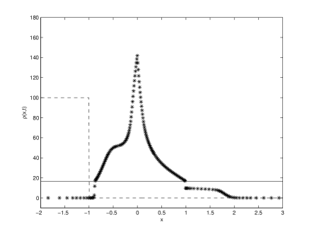
(c)	(d)

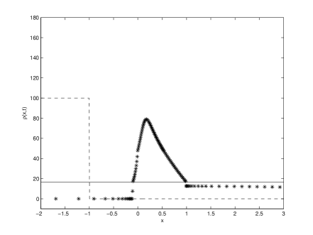
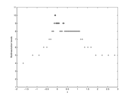
Figure 4. Example 1 (traffic model): (a, c) numerical solution and (b, d) positions of the leaves at (a, b) $t=0.05\,\mathrm{h}$ and (c, d) $t=0.1\,\mathrm{h}$.

(a)	(b)
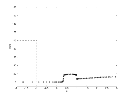
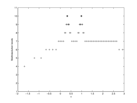
(c)	(d)

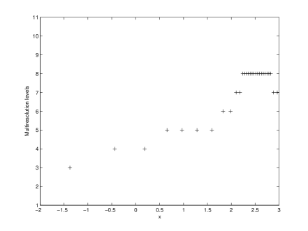
Figure 5. Example 1 (traffic model): (a, c) numerical solution and (b, d) positions of the leaves at (a, b) $t=0.15\,\mathrm{h}$ and (c, d) $t=0.2\,\mathrm{h}$.

$t_{\mathrm{final}}\,[h]$	$V$	$\eta$	$L^{1}$ error	$L^{2}$ error	$L^{\infty}$ error
0.05	6.38	4.5511	5.16$\times 10^{-4}$	6.22$\times 10^{-5}$	5.64$\times 10^{-5}\vphantom{\int^{X}}$
0.10	6.99	4.2140	4.57$\times 10^{-4}$	2.41$\times 10^{-5}$	8.16$\times 10^{-5}$
0.15	7.84	7.8168	7.21$\times 10^{-4}$	5.12$\times 10^{-5}$	7.23$\times 10^{-4}$
0.20	9.01	17.3559	1.14$\times 10^{-3}$	2.47$\times 10^{-4}$	3.86$\times 10^{-3}$

Table 1. Example 1 (traffic model): Corresponding simulated time, speed-up factor $V$, compression rate, and normalized errors. $L=10$ multiresolution levels.

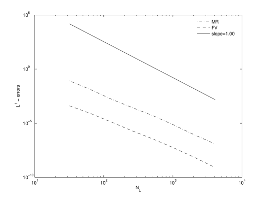
Figure 6. Example 1 (traffic model): $L^{1}$ errors.

Our numerical example for this model has been chosen in such a way that results can be compared with simulations shown in Example 5 of [16]. The velocity function is given by (2.2) with $u_{\max}=220\,\mathrm{cars}/\mathrm{mi}$, $C=\mathrm{e}/7=0.38833$ and $v_{\max}=70\,\mathrm{mph}$, so that

(6.1) $$f(u)=\begin{cases}v_{\max}u&\text{for $0\leq u\leq u_{\mathrm{c}}=\exp(-1/C)u_{\max}=16.7512\,\mathrm{cars}/\mathrm{mi}$,}\\ v_{\max}(\mathrm{e}/\mathrm{7})u\ln(u_{\max}/u)&\text{for $u_{\mathrm{c}}<u\leq u_{\max}$},\\ 0&\text{otherwise.}\end{cases}$$

We choose $v_{\max}^{0}=70$ mph and $v_{\max}^{*}=25$ mph. The initial density is chosen as

$$\rho_{0}(x)=\begin{cases}100\,\mathrm{cars}/\mathrm{mi}&\text{for $-2\,\textrm{mi}\leq x\leq-1\,\mathrm{mi}$},\\ 0&\text{otherwise.}\end{cases}$$

The integrated diffusion coefficient $A(u)$ resulting from our choice of parameters satisfies $A(u)=0$ for $0\leq u\leq u_{\mathrm{c}}=16.7512\,\mathrm{cars}/\mathrm{mi}$, and has an explicit algebraic representation [16, 58].

In Example 1, we consider an initial convoy of cars traveling on an empty road, and wish to see how the convoy passes through the reduced speed road segment. The numerical solution obtained by our method is represented in a three-dimensional plot in Figure 3 and shown at four different times in Figures 4 and 5. These figures also display the corresponding position of the leaves. For these four times, Table 1 displays the corresponding values of the speed-up factor $V$, the compression rate $\eta$, and normalized approximate errors. These errors and the speed-up factor are measured with respect to a fine grid calculation (no multiresolution) with $N_{L}=2^{13}$ cells. (We further comment on the behaviour of $V$ and $\eta$ in the discussion of Example 3.)

For this example, we take an initial dynamic graded tree, allowing $L=10$ multiresolution levels. We use a fixed time step determined by $\lambda=0.0003\,\mathrm{h}/\mathrm{mi}$, thus $\Delta t=\lambda h_{L}$. The prescribed tolerance $\varepsilon_{\mathrm{R}}$ is obtained from (5.4), where the constant $C$ for this example corresponds to a factor $C=10^{5}$, so $\varepsilon=0.301$ and the thresholding strategy is $\varepsilon_{k}=2^{k-L}\varepsilon$.

The errors in $L^{1}$ norm between the numerical solution obtained by our multiresolution scheme for different multiresolution levels $L$, and the numerical solution by finite volume approximation in a uniform fine grid with $2^{13}$ control volumes, are depicted in Fig. 6. In practice, we compute the error between the numerical solution obtained by multiresolution and the projection of the the numerical solution by finite volume approximation. We also observe the same slope ($=0.8819$) between finite volume and multiresolution computation in the $L^{1}$ error of Figure 6.

6.2. Example 2: Clarifier-thickener treating an ideal suspension ($A\equiv 0$).

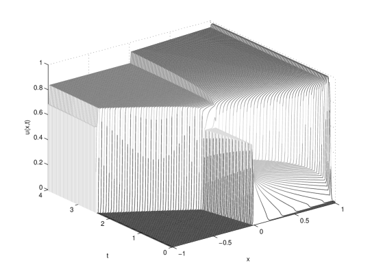
Figure 7. Example 2 (clarifier-thickener model with $A\equiv 0$): three-dimensional plot of the numerical solution.

(a)	(b)
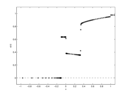
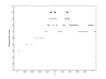
(c)	(d)

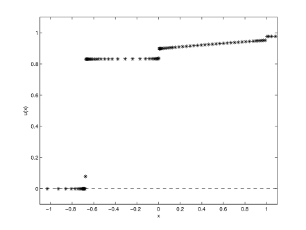
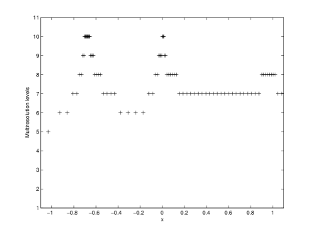
Figure 8. Example 2 (clarifier-thickener model with $A\equiv 0$): numerical solution (a, c) and position of the leaves (b, d) at $t=1$ and $t=2$.

(a)	(b)
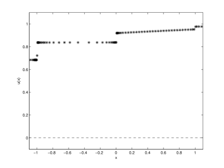
(c)	(d)

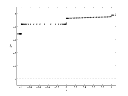
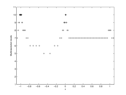
Figure 9. Example 2 (clarifier-thickener model with $A\equiv 0$): (a, c) numerical solution and (b, d) positions of the leaves at (a, b) $t=3$ and (c, d) $t=4$.

$t_{\mathrm{final}}$	$V$	$\eta$	$L^{1}$ error	$L^{2}$ error	$L^{\infty}$ error
1	8.42	6.4362	2.47$\times 10^{-4}$	6.31$\times 10^{-4}$	8.49$\times 10^{-5}\vphantom{\int^{X}}$
2	9.36	8.0315	4.11$\times 10^{-4}$	8.47$\times 10^{-4}$	2.40$\times 10^{-4}$
3	10.21	8.7850	3.42$\times 10^{-4}$	1.84$\times 10^{-3}$	6.74$\times 10^{-4}$
4	10.94	8.7850	4.18$\times 10^{-4}$	1.10$\times 10^{-3}$	1.26$\times 10^{-3}$

Table 2. Example 2 (clarifier-thickener model with $A\equiv 0$): Corresponding simulated time, speed-up factor $V$, compression rate, and normalized errors. $L=10$ multiresolution levels.

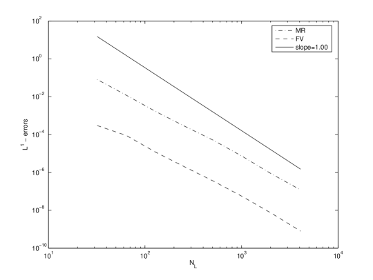
Figure 10. Example 2 (clarifier-thickener model with $A\equiv 0$): $L^{1}$ errors.

For Example 2, we choose the same parameters as in [50, 51], so that results can be compared. In particular, we consider an ideal suspension that does not form compressible sediments, i.e., we set $A\equiv 0$, so that the model considered in this example actually corresponds to the first-order equation (1.3).

We consider a clarifier-thickener unit that is initially full of water by setting $u_{0}(x)=0$. At $t=0$, we start to fill up the device with feed suspension of concentration $u_{\mathrm{F}}=0.8$. We also consider $x_{\mathrm{L}}=-1$ and $x_{\mathrm{R}}=1$ and we assume that the mixture leaving the unit at $x_{\mathrm{L}}$ and $x_{\mathrm{R}}$ is transported away at the bulk flow velocities $q_{\mathrm{L}}=-1$ and $q_{\mathrm{R}}=0.6$. The suspension is characterized by the function $f(u)$ given by (2.9) with $v_{\infty}=27/4$, $C=2$ and $u_{\max}=1$.

We use an initially graded tree with $L=10$ multiresolution levels and a reference tolerance of $\varepsilon=4.15\times 10^{-3}$. The finest grid has $N_{L}=512$ control volumes and we choose a factor $\lambda=1/16$. Observe that the visual grid used to display Figure 7 coincides with the computational grid in $x$ direction, but in $t$ direction, only every 50th profile is plotted.

For Example 2, we use as a reference solution a fine grid computation with $2^{13}$ control volumes. Table 2 lists the behaviour of the error and the gain in computational effort and data storage for different times. Also, analogously to Example 1, we can observe in Figure 10 that the plots of the $L^{1}$ error, which is measured here for $t=2$, have the same slopes.

6.3. Example 3: Clarifier-thickener treating a flocculated suspension ($A\not\equiv 0$)

Figure 11. Example 3 (clarifier-thickener treating a flocculated suspension): two views of the time-space representation of the numerical solution.

(a)	(b)
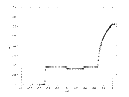
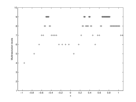
(c)	(d)

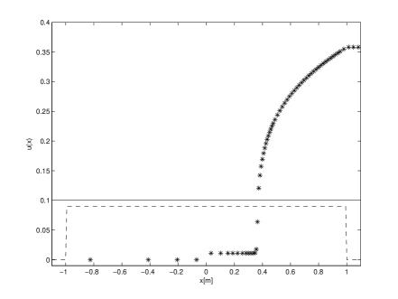
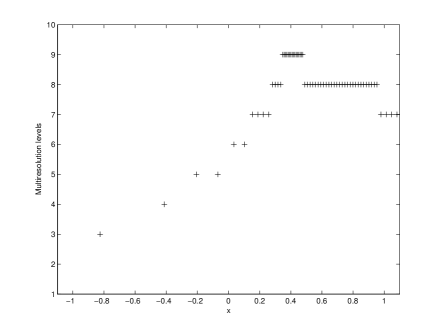
Figure 12. Example 3 (clarifier-thickener treating a flocculated suspension): (a, c) numerical solution (stars) and initial condition (dashed), (b, d) positions of the leaves (plus) at (a, b) $t=10000\,\mathrm{s}$, (c, d) $t=25000\,\mathrm{s}$ for the transition to a steady state from $u_{0}=0.09$. The horizontal solid line in (a, c) denotes the critical concentration $u_{\mathrm{c}}=0.1$.

(a)	(b)

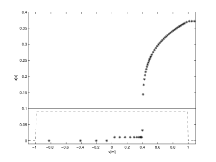
Figure 13. Example 3 (clarifier-thickener treating a flocculated suspension): (a) numerical solution (stars) and initial condition (dashed), (b) positions of the leaves (plus) at $t=50000\,\mathrm{s}$ for the transition to a steady state from $u_{0}=0.09$. The horizontal solid line in (a) denotes the critical concentration $u_{\mathrm{c}}=0.1$.

$t_{\mathrm{final}}\,[\mathrm{s}]$	$V$	$\eta$	$L^{1}$ error	$L^{2}$ error	$L^{\infty}$ error
10000	7.88	4.1787	3.67$\times 10^{-4}$	8.41$\times 10^{-5}$	6.73$\times 10^{-4}\vphantom{\int^{X}}$
25000	9.01	4.4265	4.82$\times 10^{-4}$	9.32$\times 10^{-5}$	8.29$\times 10^{-4}$
50000	10.74	4.4734	6.30$\times 10^{-4}$	1.24$\times 10^{-4}$	1.07$\times 10^{-3}$

Table 3. Example 3 (clarifier-thickener model with $A\not\equiv 0$): Corresponding simulated time, speed-up factor $V$, compression rate, and normalized errors. $L=9$ multiresolution levels.

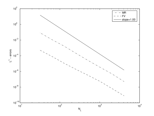
Figure 14. Example 3 (clarifier-thickener model with $A\not\equiv 0$): $L^{1}$ errors.

The parameter of the flux is the same as in Example 2, and the function $\sigma_{\!\mathrm{e}}(u)$ is given by (2.12) with $\sigma_{0}=1.0\,\mathrm{Pa}$, $u_{\mathrm{c}}=0.1$ and $\beta=6$. The remaining parameters are $\Delta_{\varrho}=1660\,\mathrm{kg}/\mathrm{m}^{3}$ and $g=9.81\,\mathrm{m}/\mathrm{s}^{2}$. Note that for (2.9) with $\beta\in\mathbb{N}$, the function $A(u)$ has an explicit closed-form representation, see [61]. The reference numerical scheme is (3.1) with $\lambda=40\,\mathrm{s}/\mathrm{m}$.

Our simulation corresponds to the choice $q_{\mathrm{R}}=2.5\times 10^{-6}\,\mathrm{m}/\mathrm{s}$ and $q_{\mathrm{L}}=-1.0\times 10^{-5}\,\mathrm{m}/\mathrm{s}$. The feed concentration corresponds to $u_{\mathrm{F}}=0.086$. Figure 11 shows the numerical solution until $t=50000\,\mathrm{s}$. In this case we consider the device with an initial concentration distribution of $u_{0}(x)=u_{\mathrm{c}}$, $x\in[x_{\mathrm{L}},x_{\mathrm{R}}]$ and we can observe the initial stage of the fill-up process. For this example, we take an initial dynamic graded tree, allowing $L=8$ multiresolution levels, and for the reference tolerance we use $C=10^{-3}$, so $\varepsilon_{\mathrm{R}}=2.24\times 10^{-4}$.

For Example 3 we use as a reference solution a fine grid computation with $2^{13}$ control volumes. Table 3 again displays the behaviour of the error and the gain in computational effort and data storage for different times. Also, analogously to the previous examples, we observe in Figure 14 the same slope between the $L^{1}$ errors for the finite volume and multiresolution methods. This error is masured here at $t=25000\,\mathrm{s}$.

Note that in all numerical examples, the speed-up factor $V$ increases as $t_{\mathrm{final}}$ is increased, even if the data compression rate $\eta$ remains constant, which approximately is the case in Table 3, or even decreases, as we see, for example, by comparing the values of $\eta$ for $t_{\mathrm{final}}=0.05\,\mathrm{h}$ and $t_{\mathrm{final}}=0.10\,\mathrm{h}$ in Table 1. The explanation of this discrepancy is that while $\eta$ measures the quality of performance of the multiresolution seen at the instant $t=t_{\mathrm{final}}$, the speed-up factor $V$ is referred to the total time of simulation and also includes the “overhead” required by initializing the graded tree in step (2) of the multiresolution algorithm. The initialization requires a fixed amount of CPU time, which is independent of the number of total time steps (which is porportional to $t_{\mathrm{final}}$, since we consider $\Delta t$ to be fixed). On the other hand, a standard FV method on a fixed grid will always require CPU time proportional to the number of time steps. This explains why even if $\eta$ does not change significantly, we observe an inprovement of the speed-up factor $V$ as $t_{\mathrm{final}}$ is increased.

7. Conclusions

Before discussing our results, we comment that the standings of both applicative models are slightly different. Numerous mathematical models have been proposed for one-directional flows of vehicular traffic; reviews of this topic are given in the monographs by Helbing [62], Kerner [63] and Garavello and Piccoli [64], as well as in the articles by Bellomo et al. [65, 66, 67]. These and other works vividly illustrate that the number of balance equations (for the car density, velocity, and possibly other flow variables) that form a time-dependent model based on partial differential equations, as well as the algebraic structure of these equations, is a topic of current research. Fortunately, all these models are spatially one-dimensional, and a circular road with periodic boundary conditions provides a setup that is both physically meaningful (since the flow is horizontal) and easy to implement for numerical simulation. This setup, on one hand, is widely used to compare different traffic models, and on the other hand allows to assess the local influence and long-term behaviour of nonlinearities and inhomogeneities such as the ones introduced in Section 6.1.

While the traffic problem highlights the use of the scheme used herein to explore different models, the clarifier-thickener model calls for an efficient tool to perform simulations, on one hand, related to clarifier-thickener design and control [20, 68], and on the other hand, to parameter identification calculations [69, 70]. In fact, depending on the parameters, clarifier-thickener operations such as fill-up may extend over weeks and months [68], and require large simulation times, while the parameter identification procedures in [69, 70] proceed by solution of an adjoint problem, which needs storage of the complete solution of the previously solved direct problem. Clearly, methods that imply savings in both computational time and memory storage, such as the multiresolution scheme presented herein, are of significant practical interest for the clarifier-thickener model.

Both mathematical models considered herein exhibit three types of fronts that typically occur in solutions of (1.2), namely standard shocks (i.e., discontinuities between solution values for both of which (1.2) is hyperbolic), hyperbolic-parabolic type-change interfaces (such as the sediment level in Example 3), and stationary discontinuities located at the discontinuities of $\boldsymbol{\gamma}(x)$. The basic motivation for applying a finite volume multiresolution scheme is that this device is is sufficiently flexible to produce the refinement necessary to properly capture all these discontinuities, and leads to considerable gains in storage as can be seen from the sparsity of the graded trees in our numerical examples. Moreover, Figure 6 confirms that we may effectively control the perturbation error, in the sense that the error of the resulting finite volume multiresolution scheme remains of the same order as that of the finite volume scheme on a uniform grid. We recall from Section 5 that the feasibility of this control depends on an estimate of the convergence rate of the basic discretization on a uniform grid, which is an open problem for strongly degenerate parabolic equations.

Although our numerical results look promising, they still alert to some shortcomings that call for improvement. The most obvious one is the limitation of the time step according to the spatial step size of the finest grid, which can possibly be removed by using a space-time adaptive scheme such as the recent finite volume multiresolution schemes by Stiriba and Müller [71]. On the other hand, the basic finite volume scheme accurately resolves the discontinuities of the solution sitting at the jumps of $\boldsymbol{\gamma}(x)$ at any level of discretization; these discontinuities are not approximated by smeared transitions (as are discontinuities at positions where $\boldsymbol{\gamma}(x)$ is smooth), see [19]. This means that the refinement the multiresolution produces near these discontinuities, which is visible in Figures 8 and 9, and which is based on the adaptation of the refinement according to features of the solution (but not of $\boldsymbol{\gamma}(x)$), is possibly unnecessary, and that a more efficient version of the present method may be feasible.

References

- [1] Harten A (1983) High resolution schemes for hyperbolic conservation laws. J Comput Phys 49:357–393
- [2] Shu CW, Osher S (1989) Efficient implementation of essentially non-oscillatory shock-capturing schemes II. J Comput Phys 83:32–78
- [3] Shu CW (1998) Essentially non-oscillatory and weighted essentially non-oscillatory schemes for hyperbolic conservation laws. In: Cockburn B, Johnson C, Shu CW, Tadmor E, Advanced Numerical Approximation of Nonlinear Hyperbolic Equations (Quarteroni A, Ed.), Lecture Notes in Mathematics vol. 1697, Springer-Verlag, Berlin (1998), 325–432
- [4] Kurganov A, Tadmor E (2000) New high resolution central schemes for nonlinear conservation laws and convection-diffusion equations. J Comput Phys 160:241–282
- [5] Nessyahu H, Tadmor E (1990) Non-oscillatory central differencing for hyperbolic conservation laws. J Comput Phys 87:408–463
- [6] Toro EF, Billett SJ (2000) Centered TVD schemes for hyperbolic conservation laws. IMA J Numer Anal 20:47–79
- [7] Harten A (1995) Multiresolution algorithms for the numerical solution of hyperbolic conservation laws. Comm Pure Appl Math 48:1305–1342
- [8] Bihari BL, Harten A (1995) Application of generalized wavelets: a multiresolution scheme. J Comp Appl Math 61:275–321
- [9] Roussel O, Schneider K, Tsigulin A, Bockhorn H (2003) A conservative fully adaptive multiresolution algorithm for parabolic PDEs. J Comput Phys 188:493–523
- [10] Dahmen W, Gottschlich-Müller B, Müller S (2001) Multiresolution schemes for conservation laws. Numer Math 88:399–443
- [11] Cohen A, Kaber SM, Müller S, Postel M (2001) Fully adaptive multiresolution finite volume schemes for conservation laws. Math Comp 72:183–225
- [12] Müller S (2003) Adaptive Multiscale Schemes for Conservation Laws. Lecture Notes in Computational Science and Engineering vol. 27, Springer-Verlag, Berlin.
- [13] Berres S, Bürger R, Karlsen KH, Tory EM (2003) Strongly degenerate parabolic-hyperbolic systems modeling polydisperse sedimentation with compression. SIAM J Appl Math 64:41–80
- [14] Bürger R, Evje S, Karlsen KH (2000) On strongly degenerate convection-diffusion problems modeling sedimentation-consolidation processes. J Math Anal Appl 247:517–556
- [15] Espedal MS, Karlsen KH (2000) Numerical solution of reservoir flow models based on large time step operator splitting methods. In: Espedal MS, Fasano A, Mikelić A (Eds.), Filtration in Porous Media and Industrial Application, Lecture Notes in Mathematics vol. 1734, Springer-Verlag, Berlin (2000), 9–77
- [16] Bürger R, Karlsen KH (2003) On a diffusively corrected kinematic-wave traffic model with changing road surface conditions. Math Models Meth Appl Sci 13:1767–1799
- [17] Nelson P (2002) Traveling-wave solutions of the diffusively corrected kinematic-wave model. Math Comp Modelling 35:561–579
- [18] Mochon S (1987) An analysis of the traffic on highways with changing surface conditions. Math Modelling 9:1–11
- [19] Bürger R, Karlsen KH, Risebro NH, Towers JD (2004) Well-posedness in and convergence of a difference scheme for continuous sedimentation in ideal clarifier-thickener units. Numer Math 97:25–65
- [20] Bürger R, Karlsen KH, Towers JD (2005) A mathematical model of continuous sedimentation of flocculated suspensions in clarifier-thickener units. SIAM J Appl Math 65:882–940
- [21] Karlsen KH, Risebro NH, Towers JD (2002) On an upwind difference scheme for degenerate parabolic convection-diffusion equations with a discontinuous coefficient. IMA J Numer Anal 22:623–664
- [22] Karlsen KH, Risebro NH, Towers JD (2003) stability for entropy solutions of nonlinear degenerate parabolic convection-diffusion equations with discontinuous coefficients. Skr K Nor Vid Selsk 3:1–49
- [23] Harten A (1994) Adaptive multiresolution schemes for shock computations. J Comput Phys 115:319–338
- [24] Harten A (1996) Multiresolution representation of data: a general framework. SIAM J Numer Anal 33:1205–1256
- [25] Jameson L (1998) A wavelet-optimized, very high order adaptive grid and order numerical method. SIAM J Sci Comput 19:1980–2013
- [26] Holmström M (1999) Solving hyperbolic PDEs using interpolating wavelets. SIAM J Sci Comput 21:405–420
- [27] Bürger R, Kozakevicius A (2007) Adaptive multiresolution WENO schemes for multi-species kinematic flow models. J Comput Phys 224:1190–1222
- [28] Verfürth R (1995) A review of A posteriori Estimation and Adaptative Mesh-Refinement Techniques. Advances in Numerical Mathematics. Wiley/Teubner, New York-Stuttgart.
- [29] Eriksson K, Hohnson C (1991) Adaptative finite element methods for parabolic problems. I. A linear model problem. SIAM J Numer Anal 28:43–77
- [30] Ohlberger M (2001) A posteriori error estimates for vertex centered finite volume approximations of convection-diffusion-reaction equations. M2AN Math Model Numer Anal 35:355–387
- [31] Tadmor E (1991) Local error estimates for discontinuous solutions of nonlinear hyperbolic equations. SIAM J Numer Anal 28:891–906
- [32] Cockburn B, Coquel F, LeFloch P (1994) An error estimate for finite volume methods for multidimensional conservation laws. Math Comp 63:77–103
- [33] Bihari BL, Harten A (1997) Multiresolution schemes for the numerical solution of 2-D conservation laws I. SIAM J Sci Comput 18:315–354
- [34] Chiavassa G, Donat R (2001) Point value multiscale algorithms for 2D compressive flows. SIAM J Sci Comput 23:805–823
- [35] Roussel O, Schneider K (2006) Numerical studies of thermodiffusive flame structures interacting with adiabatic walls using an adaptive multiresolution scheme. Combust Theory Modelling 10:273–288
- [36] Kružkov SN (1970) First order quasi-linear equations in several independent variables. Math USSR Sb 10:217–243
- [37] Vol’pert AI (1967) The spaces BV and quasilinear equations. Math USSR Sb 2:225–267
- [38] Vol’pert AI, Hudjaev SI (1969) Cauchy’s problem for degenerate second order quasilinear parabolic equations. Math USSR Sb 7:365–387
- [39] Carrillo J (1999) Entropy solutions for nonlinear degenerate problems. Arch Rat Mech Anal 147:269–361
- [40] Mascia C, Porretta A, Terracina A (2002) Nonhomogeneous Dirichlet problems for degenerate parabolic-hyperbolic equations. Arch Rat Mech Anal 163:87–124
- [41] Chen GQ, DiBenedetto E (2001) Stability of entropy solutions to the Cauchy problem for a class of nonlinear hyperbolic-parabolic equations. SIAM J Math Anal 33:751–762
- [42] Chen GQ, Perthame B (2003) Well-posedness for non-isotropic degenerate parabolic-hyperbolic equations. Ann Inst H Poincaré Anal Non Linéaire 20:645–668
- [43] Karlsen KH, Risebro NH (2003) On the uniqueness and stability of entropy solutions of nonlinear degenerate parabolic equations with rough coefficients. Discrete Contin Dyn Syst 9:1081–1104
- [44] Michel A, Vovelle J (2003) Entropy formulation for parabolic degenerate equations with general Dirichlet boundary conditions and application to the convergence of FV methods. SIAM J Numer Anal 41:2262–2293
- [45] Evje S, Karlsen KH (2000) Monotone difference approximation of solutions to degenerate convection-diffusion equations. SIAM J Numer Anal 37:1838–1860
- [46] Crandall MG, Majda A (1980) Monotone difference approximations for scalar conservation laws. Math Comp 34:1–21
- [47] Karlsen KH, Risebro NH (2001) Convergence of finite difference schemes for viscous and inviscid conservation laws with rough coefficients. M2AN Math Model Numer Anal 35:239–269
- [48] Bürger R, Coronel A, Sepúlveda M (2006) A semi-implicit monotone difference scheme for an initial-boundary value problem of a strongly degenerate parabolic equation modelling sedimentation-consolidation processes. Math Comp 75:91–112
- [49] Engquist B, Osher S (1981) One-sided difference approximations for nonlinear conservation laws. Math Comp 36:321–351
- [50] Bürger R, Karlsen KH, Klingenberg C, Risebro NH (2003) A front tracking approach to a model of continuous sedimentation in ideal clarifier-thickener units. Nonlin Anal Real World Appl 4:457–481
- [51] Bürger R, Karlsen KH, Risebro NH (2005) A relaxation scheme for continuous sedimentation in ideal clarifier-thickener units. Comput Math Appl 50:993–1009
- [52] Karlsen KH, Klingenberg C, Risebro NH (2003) A relaxation scheme for conservation laws with a discontinuous coefficient. Math Comp 73:1235–1259
- [53] Karlsen KH, Risebro NH, Towers JD (2002) On a nonlinear degenerate parabolic transport-diffusion equation with a discontinuous coefficient. Electron J Diff Eqns 93:1–23
- [54] Lighthill MJ, Whitham GB (1955) On kinematic waves. II. A theory of traffic flow on long crowded roads. Proc Roy Soc London Ser A 229:317–345
- [55] Richards PI (1956) Shock waves on the highway. Oper Res 4:42–51
- [56] Dick AC (1966) Speed/flow relationships within an urban area. Traffic Eng Control 8:393–396
- [57] Greenberg H (1959) An analysis of traffic flow. Oper Res 7:79–85
- [58] Bürger R, Kozakevicius A, Sepúlveda M (2007) Multiresolution schemes for degenerate parabolic equations in one space dimension. Numer Meth Partial Diff Eqns 23:706–730
- [59] Bürger R, Ruiz R, Schneider K, Sepúlveda M (2007) Fully adaptive multiresolution schemes for strongly degenerate parabolic equations in one space dimension. Preprint 2007-03, Departamento de Ingeniería Matemática, Universidad de Concepción; submitted.
- [60] Kuznetsov NN (1976) Accuracy of some approximate methods for computing the weak solutions of a first order quasilinear equation. USSR Comp Math and Math Phys 16:105–119
- [61] Bürger R, Karlsen KH (2001) On some upwind schemes for the phenomenological sedimentation-consolidation model. J Eng Math 41:145–166
- [62] Helbing D (1997) Verkehrsdynamik. Springer-Verlag, Berlin.
- [63] Kerner BS (2004) The Physics of Traffic. Springer-Verlag, Berlin.
- [64] Garavello M, Piccoli, B (2006) Traffic Flow on Networks. American Institute of Mathematical Sciences, Springfield, MO, USA.
- [65] Bellomo N, Coscia V (2005) First order models and closure of the mass conservation equation in the mathematical theory of vehicular traffic flow. C R Mecanique 333:843–851.
- [66] Bellomo N, Delitalia M, Coscia V (2002) On the mathematical theory of vehicular traffic flow I. Fluid dynamic and kinetic modelling. Math Models Meth Appl Sci 12:1801–1843
- [67] Bellomo N, Marasco A, Romano A (2002) From the modelling of driver’s behavior to hydrodynamic models and problems of traffic flow. Nonlin Anal Real World Appl 3:339–363
- [68] Bürger R, Narváez A (2007) Steady-state, control, and capacity calculations for flocculated suspensions in clarifier-thickeners. Int J Mineral Process, to appear.
- [69] Coronel A, James F, Sepúlveda M (2003) Numerical identification of parameters for a model of sedimentation processes. Inverse Problems 19:951–972
- [70] Berres S, Bürger R, Coronel A, Sepúlveda M (2005) Numerical identification of parameters for a strongly degenerate convection-diffusion problem modelling centrifugation of flocculated suspensions. Appl Numer Math 52:311–337
- [71] Stiriba Y, Müller S (2007) Fully adaptive multiscale schemes for conservation laws employing locally varying time stepping. J Sci Comput 30:493–531