Čech homology for shape recognition in the presence of occlusions

Abstract

In Computer Vision the ability to recognize objects in the presence of occlusions is a necessary requirement for any shape representation method. In this paper we investigate how the size function of a shape changes when a portion of the shape is occluded by another shape. More precisely, considering a set $X=A\cup B$ and a measuring function $\varphi$ on $X$, we establish a condition so that $\ell_{(X,\varphi)}=\ell_{(A,\varphi|_{A})}+\ell_{(B,\varphi|_{B})}-\ell_{(A\cap B,\varphi|_{A\cap B})}$. The main tool we use is the Mayer-Vietoris sequence of Čech homology groups. This result allows us to prove that size functions are able to detect partial matching between shapes by showing a common subset of cornerpoints.

Keywords: Size function, Mayer-Vietoris sequence, persistent homology, shape occlusion

MSC (2000): 55N05, 68U05

1 Introduction

Shape matching and retrieval are key aspects in the design of search engines based on visual, rather than keyword, information. Generally speaking, shape matching methods rely on the computation of a shape description, also called a signature, that effectively captures some essential features of the object. The ability to perform not only global matching, but also partial matching, is regarded as one of the most meaningful properties in order to evaluate the performance of a shape matching method (cf., e.g., [31]). Basically, the interest in robustness against partial occlusions is motivated by the problem of recognizing an object partially hidden by some other foreground object in the same image. However, there are also other situations in which partial matching is useful, such as when dealing with the problem of identifying similarities between different configurations of articulated objects, or when dealing with unreliable object segmentation from images. For these reasons, the ability to recognize shapes, even when they are partially occluded by another pattern, has been investigated in the Computer Vision literature by various authors, with reference to a variety of shape recognition methods (see, e.g., [7, 21, 24, 28, 29, 30]).

Size functions belong to a class of methods for shape description, characterized by the study of the topological changes in the lower level sets of a real valued function defined on the shape to derive its signature (cf., e.g., [2, 25]). In this paper we study the robustness of size functions against partial occlusions. Previous works have already assessed the robustness of size functions with respect to continuous deformations of the shape [11], the conciseness of the descriptor [19], the invariance of the descriptor to transformation groups [12, 32], that are further properties recognized as important for shape matching methods. Size functions, like most methods of their class, work on a shape as a whole. In general, it is argued that global object methods are not robust against occlusions, whereas methods based on computing local features may be more suited to this task. Our aim is to show that size functions are able to preserve local information, so that they can manage uncertainty due to the presence of occluded shapes.

We model the presence of occlusions in a shape as follows. The visible object is a locally connected compact Hausdorff space $X$. The shape of interest $A$ is occluded by a shape $B$, so that $X=A\cup B$. In particular, $A$ and $B$ have the topology induced from $X$ and are assumed to be locally connected. The shapes of $X$, $A$, and $B$ are analyzed through the size functions $\ell_{(X,\varphi)}$, $\ell_{(A,\varphi_{|A})}$, and $\ell_{(B,\varphi_{|B})}$, respectively, where $\varphi:X\rightarrow\mathbb{R}$ is the continuous function chosen to extract the shape features.

The starting point of this research is the fact that the size function $\ell_{(X,\varphi)}$, evaluated at a point $(u,v)$ of $\mathbb{R}^{2}$, with $u<v$, is equal to the rank of the image of the homomorphism induced by inclusion between the Čech homology groups $\check{H}_{0}(X_{u})$ and $\check{H}_{0}(X_{v})$, where $X_{u}=\{p\in X:\varphi(p)\leq u\}$ and $X_{v}=\{p\in X:\varphi(p)\leq v\}$.

Our main result establishes a necessary and sufficient condition so that the equality

$$\ell_{(X,\varphi)}(u,v)=\ell_{(A,\varphi_{|A})}(u,v)+\ell_{(B,\varphi_{|B})}(u,v)-\ell_{(A\cap B,\varphi_{|A\cap B})}(u,v)$$ (1)

holds. This is proved using the Mayer-Vietoris sequence of Čech homology groups.

From this result we can deduce that the size function of $X$ contains features of the size functions of $A$ and $B$. In particular, when size functions are represented as formal series of points in the plane through their cornerpoints [19], relation (1) allows us to prove that the set of cornerpoints of $\ell_{(X,\varphi)}$ contains a subset of cornerpoints of $\ell_{(A,\varphi_{|A})}$. These are a kind of “fingerprint” of the presence of $A$ in $X$. In other words, size functions are able to detect a partial matching between two shapes by showing a common subset of cornerpoints.

The paper is organized as follows. In Section 2 we introduce background notions about size functions. In Section 3 some general results concerning the link between size functions and Čech homology are proved, with a particular emphasis on the relation existing between discontinuity points of size functions [19] and homological critical values [8]. The reader not familiar with Čech homology can find a brief survey of the subject in Appendices A and B. However, we use Čech homology only for technical reasons, so that, after establishing that, in our setting, Čech homology groups satisfy all the ordinary homological axioms, we can use them as ordinary homology groups. Therefore, the reader acquainted with ordinary homology can easily go through the next sections. In Section 4 we prove our main result concerning the relationship between the size function of $A$, $B$ and $A\cup B$. The relation we obtain holds subject to a homological condition derived from the Mayer-Vietoris sequence of Čech homology. In the same section we also investigate this homological condition in terms of size functions. Moreover, we introduce the Mayer-Vietoris sequence of persistent Čech homology groups. Section 5 is devoted to the consequent relationship between cornerpoints for $\ell_{(A,\varphi|_{A})}$, $\ell_{(B,\varphi|_{B})}$ and $\ell_{(X,\varphi)}$ in terms of their coordinates and multiplicities. Before concluding the paper with a brief discussion of our results, we show some experimental applications in Section 6, demonstrating the potential of our approach.

2 Background on size functions

Size functions are a method for shape analysis that is suitable for any multi-dimensional data set that can be modeled as a topological space $X$, and whose shape properties can be described by a continuous function $\varphi$ defined on it (e.g. a domain of $\mathbb{R}^{2}$ and the height function may model terrain elevations). Size functions were introduced by P. Frosini at the beginning of the 1990s (cf., e.g., [16]), and are defined in terms of the number of connected components of lower level sets associated with the given space and function defined on it. They belong to a class of methods that are grounded in Morse theory, as described in [2]. From the theoretical point of view, the main properties of size functions that have been studied since their introduction are the computational issues [9, 17], the robustness of size functions with respect to continuous deformations of the shape [11], the conciseness of the descriptor [19], the invariance of the descriptor to transformation groups [12, 32], the connections of size functions to the natural pseudo-distance in order to compare shapes [13], their algebraic topological counterparts [5, 20], and their generalization to a setting where many functions are used at the same time to describe the same space [3]. As far as application is concerned, the most recent papers describe the retrieval of 3D objects [4] and trademark retrieval [6].

In this section we provide the reader with the necessary mathematical background concerning size functions that will be used in the next sections.

In this paper a pair $(X,\varphi)$, where $X$ denotes a non-empty compact and locally connected Hausdorff topological space, and $\varphi:X\rightarrow\mathbb{R}$ denotes a continuous function, is called a size pair. Moreover, the function $\varphi$ is called a measuring function.

Given a size pair $(X,\varphi)$, for every $u\in\mathbb{R}$, we denote by $X_{u}$ the lower level set $\{p\in X:\varphi(p)\leq u\}$.

Definition 2.1.

Let $(X,\varphi)$ be a size pair. For every $u\in\mathbb{R}$, we shall say that two points $p,q\in X$ are $\langle\varphi\leq u\rangle$-connected if and only if a connected subset of $X_{u}$ exists, containing both $p$ and $q$.

The relation of being $\langle\varphi\leq u\rangle$-connected is an equivalence relation. If two points $p,q\in X$ are $\langle\varphi\leq u\rangle$-connected we shall write $p\sim_{u}q$. For the sake of simplicity, we are going to use the same symbol $\sim_{u}$ to denote the same equivalence relation on subsets of $X$ as well.

In the following, we shall denote by $\Delta^{+}$ the open half plane $\{(u,v)\in\mathbb{R}^{2}:u<v\}$.

Definition 2.2.

The size function associated with the size pair $(X,\varphi)$ is the function $\ell_{(X,\varphi)}:\Delta^{+}\rightarrow\mathbb{N}$ such that, for every $(u,v)\in\Delta^{+}$, $\ell_{(X,\varphi)}(u,v)$ is equal to the number of equivalence classes into which the set $X_{u}$ is divided by the relation of $\langle\varphi\leq v\rangle$-connectedness.

In other words, $\ell_{({X},\varphi)}(u,v)$ is equal to the number of connected components in $X_{v}$ that contain at least one point of $X_{u}$. The finiteness of this number is a consequence of the compactness and local connectedness of $X$, and the continuity of $\varphi$.

\psfrag{P}{$P$}\psfrag{a}{$a$}\psfrag{b}{$b$}\psfrag{c}{$c$}\psfrag{e}{$e$}\psfrag{x}{$u$}\psfrag{y}{$v$}\psfrag{0}{$0$}\psfrag{1}{$1$}\psfrag{2}{$2$}\psfrag{3}{$3$}\includegraphics[width=289.07999pt]{sf.eps}

Figure 1: (b) The size function of the size pair $(X,\varphi)$, where $X$ is the curve represented by a continuous line in (a), and $\varphi$ is the function “Euclidean distance from the point $P$”.

An example of size function is illustrated in Figure 1. In this example we consider the size pair $(X,\varphi)$, where $X$ is the curve of $\mathbb{R}^{2}$, represented by a continuous line in Figure 1 (a), and $\varphi$ is the function “Euclidean distance from the point $P$”. The size function associated with $(X,\varphi)$ is shown in Figure 1 (b). Here, the domain of the size function, $\Delta^{+}$, is divided by solid lines, representing the discontinuity points of the size function. These discontinuity points divide $\Delta^{+}$ into regions where the size function is constant. The value displayed in each region is the value taken by the size function in that region.

For instance, for $a\leq u<b$, the set $X_{u}$ has two connected components contained in different connected components of $X_{v}$, when $u<v<b$. Therefore, $\ell_{\left(X,\varphi\right)}(u,v)=2$ for $a\leq u<b$ and $u<v<b$. When $a\leq u<b$ and $v\geq b$, all the connected components of $X_{u}$ are contained in the same connected component of $X_{v}$. Therefore, $\ell_{\left(X,\varphi\right)}(u,v)=1$ for $a\leq u<b$ and $v\geq b$. When $b\leq u<c$ and $v\geq c$, all of the three connected components of $X_{u}$ belong to the same connected component of $X_{v}$, implying that in this case $\ell_{\left(X,\varphi\right)}(u,v)=1$.

As for the values taken on the discontinuity lines, they are easily obtained by observing that size functions are right-continuous, both in the variable $u$ and in the variable $v$.

We point out that in less recent papers about size functions one encounters a slightly different definition of size function. In fact, the original definition of size function was based on the relation of arcwise-connectedness. The definition used in this paper, based on connectedness, was introduced in [11]. This change of definition is theoretically motivated, since it implies the right-continuity of size functions, not only in the variable $u$ but also in the variable $v$. As a consequence, many results can be stated more neatly.

An important property of size functions is that they can be represented as formal series of points, called cornerpoints. The main reference here is [19].

Definition 2.3.

For every point $p=(u,v)\in\Delta^{+}$, let us define the number $\mu_{X}(p)$ as

$$\lim_{\epsilon\to 0^{+}}\left(\ell_{(X,\varphi)}(u+\epsilon,v-\epsilon)-\ell_{(X,\varphi)}(u-\epsilon,v-\epsilon)-\ell_{(X,\varphi)}(u+\epsilon,v+\epsilon)+\ell_{(X,\varphi)}(u-\epsilon,v+\epsilon)\right).$$

The finite number $\mu_{X}(p)$ will be called multiplicity of $p$ for $\ell_{(X,\varphi)}$. Moreover, we shall call proper cornerpoint for $\ell_{(X,\varphi)}$ any point $p\in\Delta^{+}$ such that the number $\mu_{X}(p)$ is strictly positive.

Definition 2.4.

For every vertical line $r$, with equation $u=k$ in the plane $u,v$, let us identify $r$ with the pair $(k,\infty)$, and define the number $\mu_{X}(r)$ as

$$\lim_{\epsilon\to 0^{+}}\left(\ell_{(X,\varphi)}(k+\epsilon,1/\epsilon)-\ell_{(X,\varphi)}(k-\epsilon,1/\epsilon)\right).$$

When this finite number, called multiplicity of $r$ for $\ell_{(X,\varphi)}$, is strictly positive, we call $(k,\infty)$ a cornerpoint at infinity for the size function.

As an example of cornerpoints in size functions, in Figure 2 we see that the proper cornerpoints of the depicted size function are the points $p$, $q$ and $m$ (with multiplicity $2$, $1$ and $1$, respectively). The line $r$ is the only cornerpoint at infinity.

\psfrag{x}{$u$}\psfrag{y}{$v$}\psfrag{m}{$r$}\psfrag{p}{$p$}\psfrag{q}{$q$}\psfrag{s}{$s$}\psfrag{r}{$m$}\psfrag{0}{$0$}\psfrag{1}{$1$}\psfrag{3}{$3$}\psfrag{4}{$4$}\psfrag{6}{$6$}\psfrag{7}{$7$}\psfrag{5}{$5$}\includegraphics[width=144.54pt]{value.eps}

Figure 2: Cornerpoints of a size function: in this example, $p$, $q$ and $m$ are the only proper cornerpoints, and have multiplicity equal to $2$ ($p$) and $1$ ($m,q$). The point $s$ is not a cornerpoint, since its multiplicity vanishes. The line $r$ is the only cornerpoint at infinity.

The importance of cornerpoints is revealed by the next result, showing that cornerpoints, with their multiplicities, uniquely determine size functions.

The open half-plane $\Delta^{+}$, extended by the points at infinity of the kind $(k,\infty)$, will be denoted by $\Delta^{*}$, i.e.

$$\Delta^{*}:=\Delta^{+}\cup\{(k,\infty):k\in\mathbb{R}\}.$$

Theorem 2.5.

For every $({\bar{u}},{\bar{v}})\in\Delta^{+}$ we have

$$\ell_{(X,\varphi)}({\bar{u}},{\bar{v}})=\sum_{(u,v)\in\Delta^{*}\atop u\leq{\bar{u}},v>\bar{v}}\mu_{X}\big{(}(u,v)\big{)}.$$ (2)

The equality (2) can be checked in the example of Figure 2. The points where the size function takes value $0$ are exactly those for which there is no cornerpoint (either proper or at infinity) lying to the left and above them. Let us take a point in the region of the domain where the size function takes the value $3$. According to the above theorem, the value of the size function at that point must be equal to $\mu(r)+\mu(p)=3$.

3 The link between size functions and Čech homology

In this section we prove that the value of the size function can be computed in terms of rank of Čech homology groups. We then analyze the links between homological critical values and size functions.

The idea of relating size functions to homology groups is not a new one. Already in [5], introducing the concept of size functor, this link was recognized, when the space $X$ is a smooth manifold and $\varphi$ is a Morse function. Roughly speaking, the size functor associated with the pair $(X,\varphi)$ takes a pair of real numbers $(u,v)\in\Delta^{+}$ to the image of the homomorphism from $H_{k}(X_{u})$ to $H_{k}(X_{v})$, induced by inclusion of $X_{u}$ into $X_{v}$. Here homology means singular homology. This also shows a link between size functions and $0$th persistent homology groups [14]. Later, the relation between size functions and singular homology groups of closed manifolds endowed with Morse functions emerged again in [1], studying the Morse shape descriptor.

The reason for further exploring the homological interpretation of size function in the present paper is technical. As explained in Section 2, our definition of size function is based on the relation of connectedness (cf. Definition 2.2). This implies that singular homology, whose $0$th group detects the number of arcwise-connected components, is no longer suited to dealing with size functions. Adding further assumptions on $X$, so that connectedness and arcwise-connectedness coincide on $X$, such as asking $X$ to be locally arcwise-connected, is not sufficient to solve the problem. Indeed, we emphasize the fact that in the definition of $\ell_{(X,\varphi)}$ we count the components not of the space $X$ itself, but those of the lower level sets of $X$ with respect to the continuous function $\varphi$, and it is not guaranteed that locally arcwise-connectedness is inherited by lower level sets.

The tool we need for counting connected components instead of arcwise-connected components is Čech homology (a brief review of this subject can be found in Appendix A). Indeed, in [33] the following result is proved, under the assumption that $X$ is a compact Hausdorff space.

Theorem 3.1 ([33], Thm. V 11.3a).

The number of components of a space $X$ is exactly the rank of the $0$th Čech Homology group.

One of the main problems in the use of Čech homology is that, in general, the long sequence of the pair may fail to be exact. However, the exactness of this sequence holds, provided that some assumptions are satisfied: the space must be compact and the group $G$ must be either a compact Abelian topological group or a vector space over a field (see Appendix B). In view of establishing a connection between size functions and Čech homology, it is important to recall that when $(X,\varphi)$ is a size pair, $X$ is assumed to be compact and Hausdorff and $\varphi$ is continuous. Therefore, the lower level sets $X_{u}$ are themselves Hausdorff and compact spaces. In order that the Čech homology sequence of the pair be available, we will take $G$ to be a vector space over a field. Therefore, from now on, we will take the Čech homology sequence of the pair for granted and we will denote the Čech homology groups of $X$ over $G$ simply by $\check{H}_{p}(X)$, maintaining the notation $H_{p}(X)$ for ordinary homology. From [15] we know that $\check{H}_{p}(X)$ is a vector space over the same field.

We shall first furnish a link between size functions and relative Čech homology groups. We need the following preliminary results.

Definition 3.2 ([33], Def. I 12.2).

If $X$ is a space, and $x,y\in X$, then a finite collection of sets $X^{1}$, $X^{2}$, $\ldots$, $X^{n}$ will be said to form a simple chain of sets from $x$ to $y$ if (1) $X^{i}$ contains $x$ if and only if $i=1$; (2) $X^{i}$ contains $y$ if and only if $i=n$; (3) $X^{i}\cap X^{j}\neq\emptyset$, $i<j$, if and only if $j=i+1$.

Proposition 3.3 ([33], Cor. I 12.5).

A space $X$ is connected if and only if, for arbitrary $x,y\in X$ and covering $\mathcal{U}$ of $X$ by open sets, $\mathcal{U}$ contains a simple chain from $x$ to $y$.

Following the proof used in [33] to prove Theorem 3.1, we can also interpret relative homology groups in terms of the number of connected components.

Lemma 3.4.

For every pair of spaces $(X,A)$, with $X$ a compact Hausdorff space and $A$ a closed subset of $X$, the number of connected components of $X$ that do not meet $A$ is equal to the rank of $\check{H}_{0}(X,A)$.

Proof.

When $A$ is empty, the claim reduces to Theorem 3.1. When $A$ is non-empty, if $X$ is connected then $\check{H}_{0}(X,A)=0$. Indeed, under these assumptions, let $z_{0}=\{z_{0}(\mathcal{U})\}$ be a Čech cycle in $X$ relative to $A$, with $z_{0}(\mathcal{U})=\sum_{j=1}^{k}a_{j}\cdot U_{j}$, $a_{j}\neq 0$. Since $A\subseteq X$ is non-empty, there is an open set $\bar{U}\in\mathcal{U}$ such that $\bar{U}\in\mathcal{U}_{A}$. Now we can use Proposition 3.3 to show that, for every $1\leq j\leq k$, there exists a sequence ${\mathcal{S}}_{j}$ of elements of $\mathcal{U}$, beginning with $U_{j}$ and ending with $\bar{U}$. So, associated with ${\mathcal{S}}_{j}$, there is a $1$-chain $c_{1}^{j}$ such that $\partial c_{1}^{j}=U_{j}-\bar{U}$. Hence, $\partial\sum_{j=1}^{k}a_{j}\cdot c_{1}^{j}=\sum_{j=1}^{k}a_{j}\cdot U_{j}-\sum_{j=1}^{k}a_{j}\cdot\bar{U}=z_{0}(\mathcal{U})-\sum_{j=1}^{k}a_{j}\cdot\bar{U}$, proving that $z_{0}(\mathcal{U})$ is homologous to $0$ in ${Z}_{0}(X,A)$. By the arbitrariness of $\mathcal{U}$, each coordinate of $z_{0}$ is homologous to $0$, implying that $\check{H}_{0}(X,A)=0$.

In general, if $X$ is not connected, the preceding argument shows that only those connected components of $X$ that do not meet $A$ contain a non-trivial Čech cycle relative to $A$. Then the claim follows from Theorem 3.1. ∎

As an immediate consequence of Lemma 3.4, we have the following link between size functions and relative Čech homology groups. It is analogous to the link given in [1] using singular homology for size functions, defined in terms of the arcwise-connectedness relation.

Corollary 3.5.

For every size pair $(X,\varphi)$, and every $(u,v)\in\Delta^{+}$, it holds that the value $\ell_{(X,\varphi)}(u,v)$ equals the rank of $\check{H}_{0}(X_{v})$ minus the rank of $\check{H}_{0}(X_{v},X_{u})$.

Proof.

The claim follows from Lemma 3.4, observing that $\ell_{(X,\varphi)}(u,v)$ is equal to the number of connected components of $X_{v}$ that meet $X_{u}$. ∎

We now show that the size function can also be expressed as the rank of the image of the homomorphism between Čech homology groups, induced by inclusion of $X_{u}$ into $X_{v}$. This link is analogous to the existing one between the size functor and size functions, defined using the arcwise-connectedness relation [5].

Given a size pair $(X,\varphi)$, and $(u,v)\in\Delta^{+}$, we denote by $\iota^{u,v}$ the inclusion of $X_{u}$ into $X_{v}$. This mapping induces a homomorphism of Čech homology groups $\iota_{p}^{u,v}:\check{H}_{p}(X_{u})\rightarrow\check{H}_{p}(X_{v})$ for each integer $p\geq 0$.

Following [14], we can define the persistent Čech homology groups.

Definition 3.6.

Given a size pair $(X,\varphi)$ and a point $(u,v)\in\Delta^{+}$, the $p$th persistent Čech homology group $\check{H}_{p}^{u,v}$ is the image of the homomorphism $\iota_{p}^{u,v}$ induced between the $p$th Čech homology groups by the inclusion mapping of $X_{u}$ into $X_{v}$: $\mathit{\check{H}_{p}^{u,v}(X)=\mbox{\rm{im\,}}\!\iota_{p}^{u,v}}$.

Corollary 3.7.

For every size pair $(X,\varphi)$, and every $(u,v)\in\Delta^{+}$, it holds that the value $\ell_{(X,\varphi)}(u,v)$ equals the rank of the $0$th persistent Čech homology group $\check{H}_{0}^{u,v}(X)$.

Proof.

Let us consider the final terms of the long exact sequence of the pair $(X_{v},X_{u})$:

$$\ldots\rightarrow\check{H}_{0}(X_{u})\stackrel{{\scriptstyle\iota_{0}^{u,v}}}{{\rightarrow}}\check{H}_{0}(X_{v})\rightarrow\check{H}_{0}(X_{v},X_{u})\rightarrow 0.$$

From the exactness of this sequence we deduce that

$$\mbox{\rm{rank}}\check{H}_{0}^{u,v}(X)=\mbox{\rm{rank}}\mbox{\rm{im\,}}\!{\iota}_{0}^{u,v}=\mbox{\rm{rank}}\check{H}_{0}(X_{v})-\mbox{\rm{rank}}\check{H}_{0}(X_{v},X_{u}).$$

Applying Theorem 3.1 and Lemma 3.4, the rank of $\check{H}_{0}^{u,v}(X)$ turns out to be equal to the number of connected components of $X_{v}$ that meet $X_{u}$, that is $\ell_{(X,\varphi)}(u,v)$. ∎

3.1 Some useful results

In this section we show the link between homological critical values and discontinuity points of size functions. Homological critical values have been introduced in [8], and intuitively correspond to levels where the lower level sets undergo a topological change. Discontinuity points of size functions have been thoroughly studied in [19].

In particular, we prove that if a point $(u,v)\in\Delta^{+}$ is a discontinuity point for a size function, then either $u$ or $v$ is a level where the $0$-homology of the lower level set changes (Proposition 3.9). Then we show that also the converse is true when the number of homological critical values is finite (Proposition 3.10). However, in general, there may exist homological critical values not generating discontinuities for the size function (Remark 3.11). We conclude the section with a result concerning the surjectivity of the homomorphism induced by inclusion (Proposition 3.12).

Definition 3.8.

Let $(X,\varphi)$ be a size pair. A homological $p$-critical value for $(X,\varphi)$ is a real number $w$ such that, for every sufficiently small $\epsilon>0$, the map ${\iota}_{p}^{w-\epsilon,w+\epsilon}:\check{H}_{p}(X_{w-\epsilon})\rightarrow\check{H}_{p}(X_{w+\epsilon})$ induced by inclusion is not an isomorphism.

The following results show the behavior of a size function according to whether it is calculated in correspondence with homological 0-critical values or not.

Proposition 3.9.

If $w\in\mathbb{R}$ is not a homological $0$-critical value for the size pair $(X,\varphi)$, then the following statements are true:

1. For every $v>w$, $\underset{\epsilon\rightarrow 0^{+}}{\lim}\left(\ell_{(X,\varphi)}(w+\epsilon,v)-\ell_{(X,\varphi)}(w-\epsilon,v)\right)=0$;

2. For every $u<w$, $\underset{\epsilon\rightarrow 0^{+}}{\lim}\left(\ell_{(X,\varphi)}(u,w-\epsilon)-\ell_{(X,\varphi)}(u,w+\epsilon)\right)=0.$

Proof.

We begin by proving (i). Let $v>w$. For every $\epsilon>0$ such that $v>w+\epsilon$, we can consider the commutative diagram:

$$\begin{array}[]{c}\centering\hfill\lx@xy@svg{\hbox{\raise 0.0pt\hbox{\kern 6.75pt\hbox{\ignorespaces\ignorespaces\ignorespaces\hbox{\vtop{\kern 0.0pt\offinterlineskip\halign{\entry@#!@&&\entry@@#!@\cr&&&&\\&&&&\crcr}}}\ignorespaces{\hbox{\kern-6.75pt\raise 0.0pt\hbox{\hbox{\kern 0.0pt\raise 0.0pt\hbox{\hbox{\kern 3.0pt\raise 0.0pt\hbox{$\textstyle{\cdots\ignorespaces\ignorespaces\ignorespaces\ignorespaces}$}}}}}}}\ignorespaces\ignorespaces\ignorespaces\ignorespaces{}{\hbox{\lx@xy@droprule}}\ignorespaces{\hbox{\kern 31.99445pt\raise 0.0pt\hbox{\hbox{\kern 0.0pt\raise 0.0pt\hbox{\lx@xy@tip{1}\lx@xy@tip{-1}}}}}}{\hbox{\lx@xy@droprule}}{\hbox{\lx@xy@droprule}}{\hbox{\kern 31.99445pt\raise 0.0pt\hbox{\hbox{\kern 0.0pt\raise 0.0pt\hbox{\hbox{\kern 3.0pt\raise 0.0pt\hbox{$\textstyle{\check{H}_{0}(X_{w-\epsilon})\ignorespaces\ignorespaces\ignorespaces\ignorespaces\ignorespaces\ignorespaces\ignorespaces\ignorespaces}$}}}}}}}\ignorespaces\ignorespaces\ignorespaces\ignorespaces{}{\hbox{\lx@xy@droprule}}\ignorespaces\ignorespaces\ignorespaces{\hbox{\kern 83.12892pt\raise 5.58194pt\hbox{{}\hbox{\kern 0.0pt\raise 0.0pt\hbox{\hbox{\kern 3.0pt\hbox{\hbox{\kern 0.0pt\raise-1.29306pt\hbox{$\scriptstyle{{\iota}_{0}^{w-\epsilon,v}}$}}}\kern 3.0pt}}}}}}\ignorespaces{\hbox{\kern 96.18567pt\raise 0.0pt\hbox{\hbox{\kern 0.0pt\raise 0.0pt\hbox{\lx@xy@tip{1}\lx@xy@tip{-1}}}}}}{\hbox{\lx@xy@droprule}}{\hbox{\lx@xy@droprule}}\ignorespaces\ignorespaces\ignorespaces\ignorespaces{}{\hbox{\lx@xy@droprule}}\ignorespaces\ignorespaces\ignorespaces{\hbox{\kern 51.46783pt\raise-20.0pt\hbox{{}\hbox{\kern 0.0pt\raise 0.0pt\hbox{\hbox{\kern 3.0pt\hbox{\hbox{\kern 0.0pt\raise-1.44583pt\hbox{$\scriptstyle{\iota_{0}^{w-\epsilon,w+\epsilon}}$}}}\kern 3.0pt}}}}}}\ignorespaces{\hbox{\kern 51.46783pt\raise-29.5pt\hbox{\hbox{\kern 0.0pt\raise 0.0pt\hbox{\lx@xy@tip{1}\lx@xy@tip{-1}}}}}}{\hbox{\lx@xy@droprule}}{\hbox{\lx@xy@droprule}}{\hbox{\kern 96.18567pt\raise 0.0pt\hbox{\hbox{\kern 0.0pt\raise 0.0pt\hbox{\hbox{\kern 3.0pt\raise 0.0pt\hbox{$\textstyle{\check{H}_{0}(X_{v})\ignorespaces\ignorespaces\ignorespaces\ignorespaces\ignorespaces\ignorespaces\ignorespaces\ignorespaces}$}}}}}}}\ignorespaces\ignorespaces\ignorespaces\ignorespaces{}{\hbox{\lx@xy@droprule}}\ignorespaces\ignorespaces\ignorespaces{\hbox{\kern 135.8355pt\raise 5.43056pt\hbox{{}\hbox{\kern 0.0pt\raise 0.0pt\hbox{\hbox{\kern 3.0pt\hbox{\hbox{\kern 0.0pt\raise-2.43056pt\hbox{$\scriptstyle{h}$}}}\kern 3.0pt}}}}}}\ignorespaces{\hbox{\kern 154.99275pt\raise 0.0pt\hbox{\hbox{\kern 0.0pt\raise 0.0pt\hbox{\lx@xy@tip{1}\lx@xy@tip{-1}}}}}}{\hbox{\lx@xy@droprule}}{\hbox{\lx@xy@droprule}}\ignorespaces\ignorespaces\ignorespaces\ignorespaces{}{\hbox{\lx@xy@droprule}}\ignorespaces\ignorespaces\ignorespaces{\hbox{\kern 112.96698pt\raise-20.0pt\hbox{{}\hbox{\kern 0.0pt\raise 0.0pt\hbox{\hbox{\kern 3.0pt\hbox{\hbox{\kern 0.0pt\raise-1.29306pt\hbox{$\scriptstyle{\iota_{0}^{v,v}}$}}}\kern 3.0pt}}}}}}\ignorespaces{\hbox{\kern 112.96698pt\raise-29.5pt\hbox{\hbox{\kern 0.0pt\raise 0.0pt\hbox{\lx@xy@tip{1}\lx@xy@tip{-1}}}}}}{\hbox{\lx@xy@droprule}}{\hbox{\lx@xy@droprule}}{\hbox{\kern 154.99275pt\raise 0.0pt\hbox{\hbox{\kern 0.0pt\raise 0.0pt\hbox{\hbox{\kern 3.0pt\raise 0.0pt\hbox{$\textstyle{\check{H}_{0}(X_{v},X_{w-\epsilon})\ignorespaces\ignorespaces\ignorespaces\ignorespaces\ignorespaces\ignorespaces\ignorespaces\ignorespaces}$}}}}}}}\ignorespaces\ignorespaces\ignorespaces\ignorespaces{}{\hbox{\lx@xy@droprule}}\ignorespaces{\hbox{\kern 235.61319pt\raise 0.0pt\hbox{\hbox{\kern 0.0pt\raise 0.0pt\hbox{\lx@xy@tip{1}\lx@xy@tip{-1}}}}}}{\hbox{\lx@xy@droprule}}{\hbox{\lx@xy@droprule}}\ignorespaces\ignorespaces\ignorespaces\ignorespaces{}{\hbox{\lx@xy@droprule}}\ignorespaces\ignorespaces\ignorespaces{\hbox{\kern 182.68074pt\raise-20.0pt\hbox{{}\hbox{\kern 0.0pt\raise 0.0pt\hbox{\hbox{\kern 3.0pt\hbox{\hbox{\kern 0.0pt\raise-1.62779pt\hbox{$\scriptstyle{j}$}}}\kern 3.0pt}}}}}}\ignorespaces{\hbox{\kern 182.68074pt\raise-29.5pt\hbox{\hbox{\kern 0.0pt\raise 0.0pt\hbox{\lx@xy@tip{1}\lx@xy@tip{-1}}}}}}{\hbox{\lx@xy@droprule}}{\hbox{\lx@xy@droprule}}{\hbox{\kern 235.61319pt\raise 0.0pt\hbox{\hbox{\kern 0.0pt\raise 0.0pt\hbox{\hbox{\kern 3.0pt\raise 0.0pt\hbox{$\textstyle{0\ignorespaces\ignorespaces\ignorespaces\ignorespaces}$}}}}}}}\ignorespaces\ignorespaces\ignorespaces\ignorespaces{}{\hbox{\lx@xy@droprule}}\ignorespaces\ignorespaces\ignorespaces{\hbox{\kern 231.61319pt\raise-20.0pt\hbox{{}\hbox{\kern 0.0pt\raise 0.0pt\hbox{\hbox{\kern 3.0pt\hbox{\hbox{\kern 0.0pt\raise-2.25555pt\hbox{$\scriptstyle{0}$}}}\kern 3.0pt}}}}}}\ignorespaces{\hbox{\kern 241.11319pt\raise-30.55556pt\hbox{\hbox{\kern 0.0pt\raise 0.0pt\hbox{\lx@xy@tip{1}\lx@xy@tip{-1}}}}}}{\hbox{\lx@xy@droprule}}{\hbox{\lx@xy@droprule}}{\hbox{\kern-6.75pt\raise-40.0pt\hbox{\hbox{\kern 0.0pt\raise 0.0pt\hbox{\hbox{\kern 3.0pt\raise 0.0pt\hbox{$\textstyle{\cdots\ignorespaces\ignorespaces\ignorespaces\ignorespaces}$}}}}}}}\ignorespaces\ignorespaces\ignorespaces\ignorespaces{}{\hbox{\lx@xy@droprule}}\ignorespaces{\hbox{\kern 30.75pt\raise-40.0pt\hbox{\hbox{\kern 0.0pt\raise 0.0pt\hbox{\lx@xy@tip{1}\lx@xy@tip{-1}}}}}}{\hbox{\lx@xy@droprule}}{\hbox{\lx@xy@droprule}}{\hbox{\kern 30.75pt\raise-40.0pt\hbox{\hbox{\kern 0.0pt\raise 0.0pt\hbox{\hbox{\kern 3.0pt\raise 0.0pt\hbox{$\textstyle{\check{H}_{0}(X_{w+\epsilon})\ignorespaces\ignorespaces\ignorespaces\ignorespaces}$}}}}}}}\ignorespaces\ignorespaces\ignorespaces\ignorespaces{}{\hbox{\lx@xy@droprule}}\ignorespaces\ignorespaces\ignorespaces{\hbox{\kern 83.12892pt\raise-34.26529pt\hbox{{}\hbox{\kern 0.0pt\raise 0.0pt\hbox{\hbox{\kern 3.0pt\hbox{\hbox{\kern 0.0pt\raise-1.44583pt\hbox{$\scriptstyle{{\iota}_{0}^{w+\epsilon,v}}$}}}\kern 3.0pt}}}}}}\ignorespaces{\hbox{\kern 96.18567pt\raise-40.0pt\hbox{\hbox{\kern 0.0pt\raise 0.0pt\hbox{\lx@xy@tip{1}\lx@xy@tip{-1}}}}}}{\hbox{\lx@xy@droprule}}{\hbox{\lx@xy@droprule}}{\hbox{\kern 96.18567pt\raise-40.0pt\hbox{\hbox{\kern 0.0pt\raise 0.0pt\hbox{\hbox{\kern 3.0pt\raise 0.0pt\hbox{$\textstyle{\check{H}_{0}(X_{v})\ignorespaces\ignorespaces\ignorespaces\ignorespaces}$}}}}}}}\ignorespaces\ignorespaces\ignorespaces\ignorespaces{}{\hbox{\lx@xy@droprule}}\ignorespaces\ignorespaces\ignorespaces{\hbox{\kern 135.91977pt\raise-34.56944pt\hbox{{}\hbox{\kern 0.0pt\raise 0.0pt\hbox{\hbox{\kern 3.0pt\hbox{\hbox{\kern 0.0pt\raise-2.43056pt\hbox{$\scriptstyle{k}$}}}\kern 3.0pt}}}}}}\ignorespaces{\hbox{\kern 153.74829pt\raise-40.0pt\hbox{\hbox{\kern 0.0pt\raise 0.0pt\hbox{\lx@xy@tip{1}\lx@xy@tip{-1}}}}}}{\hbox{\lx@xy@droprule}}{\hbox{\lx@xy@droprule}}{\hbox{\kern 153.74829pt\raise-40.0pt\hbox{\hbox{\kern 0.0pt\raise 0.0pt\hbox{\hbox{\kern 3.0pt\raise 0.0pt\hbox{$\textstyle{\check{H}_{0}(X_{v},X_{w+\epsilon})\ignorespaces\ignorespaces\ignorespaces\ignorespaces}$}}}}}}}\ignorespaces\ignorespaces\ignorespaces\ignorespaces{}{\hbox{\lx@xy@droprule}}\ignorespaces{\hbox{\kern 235.61319pt\raise-40.0pt\hbox{\hbox{\kern 0.0pt\raise 0.0pt\hbox{\lx@xy@tip{1}\lx@xy@tip{-1}}}}}}{\hbox{\lx@xy@droprule}}{\hbox{\lx@xy@droprule}}{\hbox{\kern 235.61319pt\raise-40.0pt\hbox{\hbox{\kern 0.0pt\raise 0.0pt\hbox{\hbox{\kern 3.0pt\raise 0.0pt\hbox{$\textstyle{0}$}}}}}}}\ignorespaces}}}}\ignorespaces\hfill\@add@centering\end{array} \textstyle{\cdots\ignorespaces\ignorespaces\ignorespaces\ignorespaces} \textstyle{\check{H}_{0}(X_{w-\epsilon})\ignorespaces\ignorespaces\ignorespaces\ignorespaces\ignorespaces\ignorespaces\ignorespaces\ignorespaces} \scriptstyle{{\iota}_{0}^{w-\epsilon,v}} \scriptstyle{\iota_{0}^{w-\epsilon,w+\epsilon}} \textstyle{\check{H}_{0}(X_{v})\ignorespaces\ignorespaces\ignorespaces\ignorespaces\ignorespaces\ignorespaces\ignorespaces\ignorespaces} \scriptstyle{h} \scriptstyle{\iota_{0}^{v,v}} \textstyle{\check{H}_{0}(X_{v},X_{w-\epsilon})\ignorespaces\ignorespaces\ignorespaces\ignorespaces\ignorespaces\ignorespaces\ignorespaces\ignorespaces} \scriptstyle{j} \textstyle{0\ignorespaces\ignorespaces\ignorespaces\ignorespaces} \scriptstyle{0} \textstyle{\cdots\ignorespaces\ignorespaces\ignorespaces\ignorespaces} \textstyle{\check{H}_{0}(X_{w+\epsilon})\ignorespaces\ignorespaces\ignorespaces\ignorespaces} \scriptstyle{{\iota}_{0}^{w+\epsilon,v}} \textstyle{\check{H}_{0}(X_{v})\ignorespaces\ignorespaces\ignorespaces\ignorespaces} \scriptstyle{k} \textstyle{\check{H}_{0}(X_{v},X_{w+\epsilon})\ignorespaces\ignorespaces\ignorespaces\ignorespaces} \textstyle{0} \textstyle{\cdots\ignorespaces\ignorespaces\ignorespaces\ignorespaces} \textstyle{\check{H}_{0}(X_{w-\epsilon})\ignorespaces\ignorespaces\ignorespaces\ignorespaces\ignorespaces\ignorespaces\ignorespaces\ignorespaces} \scriptstyle{{\iota}_{0}^{w-\epsilon,v}} \scriptstyle{\iota_{0}^{w-\epsilon,w+\epsilon}} \textstyle{\check{H}_{0}(X_{v})\ignorespaces\ignorespaces\ignorespaces\ignorespaces\ignorespaces\ignorespaces\ignorespaces\ignorespaces} \scriptstyle{h} \scriptstyle{\iota_{0}^{v,v}} \textstyle{\check{H}_{0}(X_{v},X_{w-\epsilon})\ignorespaces\ignorespaces\ignorespaces\ignorespaces\ignorespaces\ignorespaces\ignorespaces\ignorespaces} \scriptstyle{j} \textstyle{0\ignorespaces\ignorespaces\ignorespaces\ignorespaces} \scriptstyle{0} \textstyle{\cdots\ignorespaces\ignorespaces\ignorespaces\ignorespaces} \textstyle{\check{H}_{0}(X_{w+\epsilon})\ignorespaces\ignorespaces\ignorespaces\ignorespaces} \scriptstyle{{\iota}_{0}^{w+\epsilon,v}} \textstyle{\check{H}_{0}(X_{v})\ignorespaces\ignorespaces\ignorespaces\ignorespaces} \scriptstyle{k} \textstyle{\check{H}_{0}(X_{v},X_{w+\epsilon})\ignorespaces\ignorespaces\ignorespaces\ignorespaces} \textstyle{0}$$ (8)

where the two horizontal lines are exact homology sequences of the pairs $(X_{v},X_{w-\epsilon})$ and $(X_{v},X_{w+\epsilon})$, respectively, and the vertical maps are homomorphisms induced by inclusions. By the assumption that $w$ is not a homological 0-critical value, there exists an arbitrarily small $\overline{\epsilon}>0$ such that $\iota_{0}^{w-\overline{\epsilon},w+\overline{\epsilon}}$ is an isomorphism. Therefore, by applying the Five Lemma in diagram (8) with $\epsilon=\overline{\epsilon}$, we deduce that $j$ is an isomorphism. Thus, $\mbox{\rm{rank}}\check{H}_{0}(X_{v},X_{w-\overline{\epsilon}})=\mbox{\rm{rank}}\check{H}_{0}(X_{v},X_{w+\overline{\epsilon}})$, and consequently, by Corollary 3.5, $\ell_{(X,\varphi)}(w+\overline{\epsilon},v)=\ell_{(X,\varphi)}(w-\overline{\epsilon},v).$ Hence, since size functions are non-decreasing in the first variable, it may be concluded that $\underset{\epsilon\rightarrow 0^{+}}{\lim}\left(\ell_{(X,\varphi)}(w+\epsilon,v)-\ell_{(X,\varphi)}(w-\epsilon,v)\right)=0$.

Now, let us proceed by proving (ii). Let $u<w$. For every $\epsilon>0$ such that $u<w-\epsilon$, let us consider the following commutative diagram:

$$\begin{array}[]{c}\centering\hfill\lx@xy@svg{\hbox{\raise 0.0pt\hbox{\kern 6.75pt\hbox{\ignorespaces\ignorespaces\ignorespaces\hbox{\vtop{\kern 0.0pt\offinterlineskip\halign{\entry@#!@&&\entry@@#!@\cr&&&&\\&&&&\crcr}}}\ignorespaces{\hbox{\kern-6.75pt\raise 0.0pt\hbox{\hbox{\kern 0.0pt\raise 0.0pt\hbox{\hbox{\kern 3.0pt\raise 0.0pt\hbox{$\textstyle{\cdots\ignorespaces\ignorespaces\ignorespaces\ignorespaces}$}}}}}}}\ignorespaces\ignorespaces\ignorespaces\ignorespaces{}{\hbox{\lx@xy@droprule}}\ignorespaces{\hbox{\kern 30.75pt\raise 0.0pt\hbox{\hbox{\kern 0.0pt\raise 0.0pt\hbox{\lx@xy@tip{1}\lx@xy@tip{-1}}}}}}{\hbox{\lx@xy@droprule}}{\hbox{\lx@xy@droprule}}{\hbox{\kern 30.75pt\raise 0.0pt\hbox{\hbox{\kern 0.0pt\raise 0.0pt\hbox{\hbox{\kern 3.0pt\raise 0.0pt\hbox{$\textstyle{\check{H}_{0}(X_{u})\ignorespaces\ignorespaces\ignorespaces\ignorespaces\ignorespaces\ignorespaces\ignorespaces\ignorespaces}$}}}}}}}\ignorespaces\ignorespaces\ignorespaces\ignorespaces{}{\hbox{\lx@xy@droprule}}\ignorespaces\ignorespaces\ignorespaces{\hbox{\kern 76.34229pt\raise 5.58194pt\hbox{{}\hbox{\kern 0.0pt\raise 0.0pt\hbox{\hbox{\kern 3.0pt\hbox{\hbox{\kern 0.0pt\raise-1.29306pt\hbox{$\scriptstyle{\iota_{0}^{u,w-\epsilon}}$}}}\kern 3.0pt}}}}}}\ignorespaces{\hbox{\kern 89.84744pt\raise 0.0pt\hbox{\hbox{\kern 0.0pt\raise 0.0pt\hbox{\lx@xy@tip{1}\lx@xy@tip{-1}}}}}}{\hbox{\lx@xy@droprule}}{\hbox{\lx@xy@droprule}}\ignorespaces\ignorespaces\ignorespaces\ignorespaces{}{\hbox{\lx@xy@droprule}}\ignorespaces\ignorespaces\ignorespaces{\hbox{\kern 47.6765pt\raise-20.0pt\hbox{{}\hbox{\kern 0.0pt\raise 0.0pt\hbox{\hbox{\kern 3.0pt\hbox{\hbox{\kern 0.0pt\raise-1.29306pt\hbox{$\scriptstyle{\iota_{0}^{u,u}}$}}}\kern 3.0pt}}}}}}\ignorespaces{\hbox{\kern 47.6765pt\raise-29.5pt\hbox{\hbox{\kern 0.0pt\raise 0.0pt\hbox{\lx@xy@tip{1}\lx@xy@tip{-1}}}}}}{\hbox{\lx@xy@droprule}}{\hbox{\lx@xy@droprule}}{\hbox{\kern 89.84744pt\raise 0.0pt\hbox{\hbox{\kern 0.0pt\raise 0.0pt\hbox{\hbox{\kern 3.0pt\raise 0.0pt\hbox{$\textstyle{\check{H}_{0}(X_{w-\epsilon})\ignorespaces\ignorespaces\ignorespaces\ignorespaces\ignorespaces\ignorespaces\ignorespaces\ignorespaces}$}}}}}}}\ignorespaces\ignorespaces\ignorespaces\ignorespaces{}{\hbox{\lx@xy@droprule}}\ignorespaces\ignorespaces\ignorespaces{\hbox{\kern 137.51201pt\raise 5.43056pt\hbox{{}\hbox{\kern 0.0pt\raise 0.0pt\hbox{\hbox{\kern 3.0pt\hbox{\hbox{\kern 0.0pt\raise-2.43056pt\hbox{$\scriptstyle{h}$}}}\kern 3.0pt}}}}}}\ignorespaces{\hbox{\kern 155.28311pt\raise 0.0pt\hbox{\hbox{\kern 0.0pt\raise 0.0pt\hbox{\lx@xy@tip{1}\lx@xy@tip{-1}}}}}}{\hbox{\lx@xy@droprule}}{\hbox{\lx@xy@droprule}}\ignorespaces\ignorespaces\ignorespaces\ignorespaces{}{\hbox{\lx@xy@droprule}}\ignorespaces\ignorespaces\ignorespaces{\hbox{\kern 109.32083pt\raise-20.0pt\hbox{{}\hbox{\kern 0.0pt\raise 0.0pt\hbox{\hbox{\kern 3.0pt\hbox{\hbox{\kern 0.0pt\raise-1.44583pt\hbox{$\scriptstyle{\iota_{0}^{w-\epsilon,w+\epsilon}}$}}}\kern 3.0pt}}}}}}\ignorespaces{\hbox{\kern 109.32083pt\raise-29.5pt\hbox{\hbox{\kern 0.0pt\raise 0.0pt\hbox{\lx@xy@tip{1}\lx@xy@tip{-1}}}}}}{\hbox{\lx@xy@droprule}}{\hbox{\lx@xy@droprule}}{\hbox{\kern 155.28311pt\raise 0.0pt\hbox{\hbox{\kern 0.0pt\raise 0.0pt\hbox{\hbox{\kern 3.0pt\raise 0.0pt\hbox{$\textstyle{\check{H}_{0}(X_{w-\epsilon},X_{u})\ignorespaces\ignorespaces\ignorespaces\ignorespaces\ignorespaces\ignorespaces\ignorespaces\ignorespaces}$}}}}}}}\ignorespaces\ignorespaces\ignorespaces\ignorespaces{}{\hbox{\lx@xy@droprule}}\ignorespaces{\hbox{\kern 236.19394pt\raise 0.0pt\hbox{\hbox{\kern 0.0pt\raise 0.0pt\hbox{\lx@xy@tip{1}\lx@xy@tip{-1}}}}}}{\hbox{\lx@xy@droprule}}{\hbox{\lx@xy@droprule}}\ignorespaces\ignorespaces\ignorespaces\ignorespaces{}{\hbox{\lx@xy@droprule}}\ignorespaces\ignorespaces\ignorespaces{\hbox{\kern 183.1163pt\raise-20.0pt\hbox{{}\hbox{\kern 0.0pt\raise 0.0pt\hbox{\hbox{\kern 3.0pt\hbox{\hbox{\kern 0.0pt\raise-1.62779pt\hbox{$\scriptstyle{j}$}}}\kern 3.0pt}}}}}}\ignorespaces{\hbox{\kern 183.1163pt\raise-29.5pt\hbox{\hbox{\kern 0.0pt\raise 0.0pt\hbox{\lx@xy@tip{1}\lx@xy@tip{-1}}}}}}{\hbox{\lx@xy@droprule}}{\hbox{\lx@xy@droprule}}{\hbox{\kern 236.19394pt\raise 0.0pt\hbox{\hbox{\kern 0.0pt\raise 0.0pt\hbox{\hbox{\kern 3.0pt\raise 0.0pt\hbox{$\textstyle{0\ignorespaces\ignorespaces\ignorespaces\ignorespaces}$}}}}}}}\ignorespaces\ignorespaces\ignorespaces\ignorespaces{}{\hbox{\lx@xy@droprule}}\ignorespaces\ignorespaces\ignorespaces{\hbox{\kern 232.19394pt\raise-20.0pt\hbox{{}\hbox{\kern 0.0pt\raise 0.0pt\hbox{\hbox{\kern 3.0pt\hbox{\hbox{\kern 0.0pt\raise-2.25555pt\hbox{$\scriptstyle{0}$}}}\kern 3.0pt}}}}}}\ignorespaces{\hbox{\kern 241.69394pt\raise-30.55556pt\hbox{\hbox{\kern 0.0pt\raise 0.0pt\hbox{\lx@xy@tip{1}\lx@xy@tip{-1}}}}}}{\hbox{\lx@xy@droprule}}{\hbox{\lx@xy@droprule}}{\hbox{\kern-6.75pt\raise-40.0pt\hbox{\hbox{\kern 0.0pt\raise 0.0pt\hbox{\hbox{\kern 3.0pt\raise 0.0pt\hbox{$\textstyle{\cdots\ignorespaces\ignorespaces\ignorespaces\ignorespaces}$}}}}}}}\ignorespaces\ignorespaces\ignorespaces\ignorespaces{}{\hbox{\lx@xy@droprule}}\ignorespaces{\hbox{\kern 30.75pt\raise-40.0pt\hbox{\hbox{\kern 0.0pt\raise 0.0pt\hbox{\lx@xy@tip{1}\lx@xy@tip{-1}}}}}}{\hbox{\lx@xy@droprule}}{\hbox{\lx@xy@droprule}}{\hbox{\kern 30.75pt\raise-40.0pt\hbox{\hbox{\kern 0.0pt\raise 0.0pt\hbox{\hbox{\kern 3.0pt\raise 0.0pt\hbox{$\textstyle{\check{H}_{0}(X_{u})\ignorespaces\ignorespaces\ignorespaces\ignorespaces}$}}}}}}}\ignorespaces\ignorespaces\ignorespaces\ignorespaces{}{\hbox{\lx@xy@droprule}}\ignorespaces\ignorespaces\ignorespaces{\hbox{\kern 76.34229pt\raise-34.26529pt\hbox{{}\hbox{\kern 0.0pt\raise 0.0pt\hbox{\hbox{\kern 3.0pt\hbox{\hbox{\kern 0.0pt\raise-1.44583pt\hbox{$\scriptstyle{\iota_{0}^{u,w+\epsilon}}$}}}\kern 3.0pt}}}}}}\ignorespaces{\hbox{\kern 88.603pt\raise-40.0pt\hbox{\hbox{\kern 0.0pt\raise 0.0pt\hbox{\lx@xy@tip{1}\lx@xy@tip{-1}}}}}}{\hbox{\lx@xy@droprule}}{\hbox{\lx@xy@droprule}}{\hbox{\kern 88.603pt\raise-40.0pt\hbox{\hbox{\kern 0.0pt\raise 0.0pt\hbox{\hbox{\kern 3.0pt\raise 0.0pt\hbox{$\textstyle{\check{H}_{0}(X_{w+\epsilon})\ignorespaces\ignorespaces\ignorespaces\ignorespaces}$}}}}}}}\ignorespaces\ignorespaces\ignorespaces\ignorespaces{}{\hbox{\lx@xy@droprule}}\ignorespaces\ignorespaces\ignorespaces{\hbox{\kern 137.59628pt\raise-34.56944pt\hbox{{}\hbox{\kern 0.0pt\raise 0.0pt\hbox{\hbox{\kern 3.0pt\hbox{\hbox{\kern 0.0pt\raise-2.43056pt\hbox{$\scriptstyle{k}$}}}\kern 3.0pt}}}}}}\ignorespaces{\hbox{\kern 154.03867pt\raise-40.0pt\hbox{\hbox{\kern 0.0pt\raise 0.0pt\hbox{\lx@xy@tip{1}\lx@xy@tip{-1}}}}}}{\hbox{\lx@xy@droprule}}{\hbox{\lx@xy@droprule}}{\hbox{\kern 154.03867pt\raise-40.0pt\hbox{\hbox{\kern 0.0pt\raise 0.0pt\hbox{\hbox{\kern 3.0pt\raise 0.0pt\hbox{$\textstyle{\check{H}_{0}(X_{w+\epsilon},X_{u})\ignorespaces\ignorespaces\ignorespaces\ignorespaces}$}}}}}}}\ignorespaces\ignorespaces\ignorespaces\ignorespaces{}{\hbox{\lx@xy@droprule}}\ignorespaces{\hbox{\kern 236.19394pt\raise-40.0pt\hbox{\hbox{\kern 0.0pt\raise 0.0pt\hbox{\lx@xy@tip{1}\lx@xy@tip{-1}}}}}}{\hbox{\lx@xy@droprule}}{\hbox{\lx@xy@droprule}}{\hbox{\kern 236.19394pt\raise-40.0pt\hbox{\hbox{\kern 0.0pt\raise 0.0pt\hbox{\hbox{\kern 3.0pt\raise 0.0pt\hbox{$\textstyle{0}$}}}}}}}\ignorespaces}}}}\ignorespaces\hfill\@add@centering\end{array} \textstyle{\cdots\ignorespaces\ignorespaces\ignorespaces\ignorespaces} \textstyle{\check{H}_{0}(X_{u})\ignorespaces\ignorespaces\ignorespaces\ignorespaces\ignorespaces\ignorespaces\ignorespaces\ignorespaces} \scriptstyle{\iota_{0}^{u,w-\epsilon}} \scriptstyle{\iota_{0}^{u,u}} \textstyle{\check{H}_{0}(X_{w-\epsilon})\ignorespaces\ignorespaces\ignorespaces\ignorespaces\ignorespaces\ignorespaces\ignorespaces\ignorespaces} \scriptstyle{h} \scriptstyle{\iota_{0}^{w-\epsilon,w+\epsilon}} \textstyle{\check{H}_{0}(X_{w-\epsilon},X_{u})\ignorespaces\ignorespaces\ignorespaces\ignorespaces\ignorespaces\ignorespaces\ignorespaces\ignorespaces} \scriptstyle{j} \textstyle{0\ignorespaces\ignorespaces\ignorespaces\ignorespaces} \scriptstyle{0} \textstyle{\cdots\ignorespaces\ignorespaces\ignorespaces\ignorespaces} \textstyle{\check{H}_{0}(X_{u})\ignorespaces\ignorespaces\ignorespaces\ignorespaces} \scriptstyle{\iota_{0}^{u,w+\epsilon}} \textstyle{\check{H}_{0}(X_{w+\epsilon})\ignorespaces\ignorespaces\ignorespaces\ignorespaces} \scriptstyle{k} \textstyle{\check{H}_{0}(X_{w+\epsilon},X_{u})\ignorespaces\ignorespaces\ignorespaces\ignorespaces} \textstyle{0} \textstyle{\cdots\ignorespaces\ignorespaces\ignorespaces\ignorespaces} \textstyle{\check{H}_{0}(X_{u})\ignorespaces\ignorespaces\ignorespaces\ignorespaces\ignorespaces\ignorespaces\ignorespaces\ignorespaces} \scriptstyle{\iota_{0}^{u,w-\epsilon}} \scriptstyle{\iota_{0}^{u,u}} \textstyle{\check{H}_{0}(X_{w-\epsilon})\ignorespaces\ignorespaces\ignorespaces\ignorespaces\ignorespaces\ignorespaces\ignorespaces\ignorespaces} \scriptstyle{h} \scriptstyle{\iota_{0}^{w-\epsilon,w+\epsilon}} \textstyle{\check{H}_{0}(X_{w-\epsilon},X_{u})\ignorespaces\ignorespaces\ignorespaces\ignorespaces\ignorespaces\ignorespaces\ignorespaces\ignorespaces} \scriptstyle{j} \textstyle{0\ignorespaces\ignorespaces\ignorespaces\ignorespaces} \scriptstyle{0} \textstyle{\cdots\ignorespaces\ignorespaces\ignorespaces\ignorespaces} \textstyle{\check{H}_{0}(X_{u})\ignorespaces\ignorespaces\ignorespaces\ignorespaces} \scriptstyle{\iota_{0}^{u,w+\epsilon}} \textstyle{\check{H}_{0}(X_{w+\epsilon})\ignorespaces\ignorespaces\ignorespaces\ignorespaces} \scriptstyle{k} \textstyle{\check{H}_{0}(X_{w+\epsilon},X_{u})\ignorespaces\ignorespaces\ignorespaces\ignorespaces} \textstyle{0}$$ (14)

where the vertical maps are homomorphisms induced by inclusions and the two horizontal lines are exact homology sequences of the pairs $(X_{w-\epsilon},X_{u})$ and $(X_{w+\epsilon},X_{u})$, respectively. By the assumption that $w$ is not a homological 0-critical value, there exists an arbitrarily small $\overline{\epsilon}>0$, for which ${\iota}_{0}^{w-\overline{\epsilon},w+\overline{\epsilon}}:\check{H}_{0}(X_{w-\overline{\epsilon}})\rightarrow\check{H}_{0}(X_{w+\overline{\epsilon}})$ is an isomorphism. Therefore, by applying the Five Lemma in diagram (14) with $\epsilon=\overline{\epsilon}$, we deduce that $j$ is an isomorphism. Thus, $\mbox{\rm{rank}}\check{H}_{0}(X_{w-\overline{\epsilon}},X_{u})=\mbox{\rm{rank}}\check{H}_{0}(X_{w+\overline{\epsilon}},X_{u})$, implying $\ell_{(X,\varphi)}(u,w-\overline{\epsilon})=\ell_{(X,\varphi)}(u,w+\overline{\epsilon})$. Hence, since size functions are non-increasing in the second variable, the desired claim follows. ∎

Assuming the existence of at most a finite number of homological critical values, we can say that homological critical values give rise to discontinuities in size functions.

Proposition 3.10.

Let $(X,\varphi)$ be a size pair with at most a finite number of homological 0-critical values. Let $w\in\mathbb{R}$ be a homological 0-critical value. The following statements hold:

1. If ${\iota}_{0}^{w-\epsilon,w+\epsilon}$ is not surjective for any sufficiently small positive real number $\epsilon$, then there exists $v>w$ such that $w$ is a discontinuity point for $\ell_{(X,\varphi)}(\cdot,v)$;

2. If ${\iota}_{0}^{w-\epsilon,w+\epsilon}$ is surjective for every sufficiently small positive real number $\epsilon$, then there exists $u<w$ such that $w$ is a discontinuity point for $\ell_{(X,\varphi)}(u,\cdot)$.

Proof.

Let us prove (i), always referring to diagram (8) in the proof of Proposition 3.9. Let $v>w$. For every $\epsilon>0$ such that $v>w+\epsilon$, the map $j$ of diagram (8) is surjective. Indeed, $h$, $k$ and $\iota_{0}^{v,v}$ are surjective.

If we prove that there exists $v>w$ for which, for every $\epsilon>0$ such that $v>w+\epsilon$, $j$ is not injective, then, since $j$ is surjective, it necessarily holds that $\mbox{\rm{rank}}\check{H}_{0}(X_{v},X_{w-\epsilon})>\mbox{\rm{rank}}\check{H}_{0}(X_{v},X_{w+\epsilon})$, for every $\epsilon>0$ such that $v>w+\epsilon$. From this we obtain $\ell_{(X,\varphi)}(w-\epsilon,v)=\mbox{\rm{rank}}\check{H}_{0}(X_{v})-\mbox{\rm{rank}}\check{H}_{0}(X_{v},X_{w-\epsilon})<\mbox{\rm{rank}}\check{H}_{0}(X_{v})-\mbox{\rm{rank}}\check{H}_{0}(X_{v},X_{w+\epsilon})=\ell_{(X,\varphi)}(w+\epsilon,v)$, for every $\epsilon>0$ such that $v>w+\epsilon$. Therefore, $\underset{\epsilon\rightarrow 0^{+}}{\lim}\left(\ell_{(X,\varphi)}(w+\epsilon,v)-\ell_{(X,\varphi)}(w-\epsilon,v)\right)>0$, that is, $w$ is a discontinuity point for $\ell_{(X,\varphi)}(\cdot,v)$.

We now show that there exists $v>w$ for which, for every $\epsilon>0$ such that $v>w+\epsilon$, $j$ is not injective.
Since we have hypothesized the presence of at most a finite number of homological 0-critical values for $(X,\varphi)$, there surely exists $v>w$ such that, for every sufficiently small $\epsilon>0$, $v>w+\epsilon$ and ${\iota}_{0}^{w+\epsilon,v}:\check{H}_{0}(X_{w+\epsilon})\rightarrow\check{H}_{0}(X_{v})$ is an isomorphism. Hence, from the exactness of the second row in diagram (8), taking such a $v$, $\check{H}_{0}(X_{v},X_{w+\epsilon})$ is trivial. Now, if $j$ were injective, from the triviality of $\check{H}_{0}(X_{v},X_{w+\epsilon})$, it would follow that $\check{H}_{0}(X_{v},X_{w-\epsilon})$ is also trivial, and consequently ${\iota}_{0}^{w-\epsilon,v}$ surjective. This is a contradiction, since we are assuming $\iota_{0}^{w-\epsilon,w+\epsilon}$ not surjective, and it implies that ${\iota}_{0}^{w-\epsilon,v}$ is not surjective because $\iota_{0}^{w+\epsilon,v}$ and $\iota_{0}^{v,v}$ are isomorphisms.

As for (ii), we will always refer to diagram (14) in the proof of Proposition 3.9. In this case, by combining the hypothesis that, for any sufficiently small $\epsilon>0$, ${\iota}_{0}^{w-\epsilon,w+\epsilon}$ is not an isomorphism and ${\iota}_{0}^{w-\epsilon,w+\epsilon}$ is surjective, it necessarily follows that ${\iota}_{0}^{w-\epsilon,w+\epsilon}$ is not injective. Hence, $\mbox{\rm{rank}}\check{H}_{0}(X_{w-\epsilon})>\mbox{\rm{rank}}\check{H}_{0}(X_{w+\epsilon})$, for every sufficiently small $\epsilon>0$. Let $u<w$. For every $\epsilon>0$ such that $u+\epsilon<w$, the map $j$ of diagram (14) is surjective. Indeed, $h$, $k$ and $\iota_{0}^{w-\epsilon,w+\epsilon}$ are surjective.

Now, if we prove the existence of $u<w$, for which, for every $\epsilon>0$ such that $u+\epsilon<w$, $j$ is an isomorphism, it necessarily holds that $\mbox{\rm{rank}}\check{H}_{0}(X_{w-\epsilon},X_{u})=\mbox{\rm{rank}}\check{H}_{0}(X_{w+\epsilon},X_{u})$, for every $\epsilon>0$ such that $u+\epsilon<w$. Thus, it follows that $\ell_{(X,\varphi)}(u,w-\epsilon)=\mbox{\rm{rank}}\check{H}_{0}(X_{w-\epsilon})-\mbox{\rm{rank}}\check{H}_{0}(X_{w-\epsilon},X_{u})>\mbox{\rm{rank}}\check{H}_{0}(X_{w+\epsilon})-\mbox{\rm{rank}}\check{H}_{0}(X_{w+\epsilon},X_{u})=\ell_{(X,\varphi)}(u,w+\epsilon)$, for every $\epsilon>0$ such that $u+\epsilon<w$, implying $\underset{\epsilon\rightarrow 0^{+}}{\lim}\left(\ell_{(X,\varphi)}(u,w-\epsilon)-\ell_{(X,\varphi)}(u,w+\epsilon)\right)>0$, that is, $w$ is a discontinuity point for $\ell_{(X,\varphi)}(u,\cdot)$.

Recalling that $j$ is surjective, let us prove that there exists $u<w$ for which $j$ is injective for every $\epsilon>0$ with $u+\epsilon<w$.
Since we have assumed the presence of at most a finite number of homological 0-critical values for $(X,\varphi)$, there surely exists $u<w$ such that, for every sufficiently small $\epsilon>0$, $u<w-\epsilon$ and ${\iota}_{0}^{u,w-\epsilon}:\check{H}_{0}(X_{u})\rightarrow\check{H}_{0}(X_{w-\epsilon})$ is an isomorphism. Hence, for such a $u$, $\check{H}_{0}(X_{w-\epsilon},X_{u})$ is trivial, implying $j$ injective. ∎

Dropping the assumption that the number of homological 0-critical values for $(X,\varphi)$ is finite, the converse of Proposition 3.9 is false, as the following remark states.

Remark 3.11.

From the condition that $w$ is a homological 0-critical value, it does not follow that $w$ is a discontinuity point for the function $\ell_{(X,\varphi)}(\cdot,v)$, $v>w$, or for the function $\ell_{(X,\varphi)}(u,\cdot)$, $u<w$.

In particular, the hypothesis $\mbox{\rm{rank}}\check{H}_{0}(X_{w-\epsilon})\neq\mbox{\rm{rank}}\check{H}_{0}(X_{w+\epsilon})$, for every sufficiently small $\epsilon>0$, does not imply that there exists either $v>w$ such that $\underset{\epsilon\rightarrow 0^{+}}{\lim}\left(\ell_{(X,\varphi)}(w+\epsilon,v)-\ell_{(X,\varphi)}(w-\epsilon,v)\right)\neq 0$ or $u<w$ such that
$\underset{\epsilon\rightarrow 0^{+}}{\lim}\left(\ell_{(X,\varphi)}(u,w-\epsilon)-\ell_{(X,\varphi)}(u,w+\epsilon)\right)\neq 0.$

\psfrag{a}{$\scriptstyle{1}$}\psfrag{b}{$\scriptstyle{9/8}$}\psfrag{c}{$\scriptstyle{5/4}$}\psfrag{d}{$\scriptstyle{3/2}$}\psfrag{u}{$\scriptstyle{u}$}\psfrag{v}{$\scriptstyle{v}$}\psfrag{0}{$\scriptstyle{0}$}\psfrag{1}{$\scriptstyle{1}$}\psfrag{2}{$\scriptstyle{2}$}\psfrag{e}{$\scriptstyle{2}$}\includegraphics[height=113.81102pt]{patologicEx1.eps}	\psfrag{a}{$\scriptstyle{1}$}\psfrag{b}{$\scriptstyle{3/2}$}\psfrag{c}{$\scriptstyle{7/4}$}\psfrag{d}{$\scriptstyle{15/8}$}\psfrag{u}{$\scriptstyle{u}$}\psfrag{v}{$\scriptstyle{v}$}\psfrag{0}{$\scriptstyle{0}$}\psfrag{1}{$\scriptstyle{1}$}\psfrag{2}{$\scriptstyle{2}$}\psfrag{e}{$\scriptstyle{2}$}\includegraphics[height=113.81102pt]{patologicEx2.eps}
$(a)$	$(b)$

Figure 3: Two examples showing the existence of a real number $w$ that is a homological 0-critical value for $(X,\varphi)$ but not a discontinuity point for $\ell_{(X,\varphi)}(\cdot,v)$ or $\ell_{(X,\varphi)}(u,\cdot)$.

Two different examples, shown in Figure 3, support our claim.

Let us describe the first example (see Figure 3, (a)). Let $(X,\varphi)$ be the size pair where $X$ is the topological space obtained by adding an infinite number of branches to a vertical segment, each one sprouting at the height where the previous expires. These heights are chosen according to the sequence $(1+\frac{1}{2^{n}})_{n\in\mathbb{N}}$, converging to $1$. The measuring function $\varphi$ is the height function. The size function associated with $(X,\varphi)$ is displayed on the right side of $X$. In this case, $w=1$ is a homological 0-critical value. Indeed, for $w=1$, it holds that $\mbox{\rm{rank}}\check{H}_{0}(X_{w-\epsilon})=1$ while $\mbox{\rm{rank}}\check{H}_{0}(X_{w+\epsilon})=2$, for every sufficiently small $\epsilon>0$. On the other hand, for every $v>w$, and for every small enough $\epsilon>0$, it holds that $\ell_{(X,\varphi)}(w+\epsilon,v)=\ell_{(X,\varphi)}(w-\epsilon,v)=1$. Therefore, $\underset{\epsilon\rightarrow 0^{+}}{\lim}\left(\ell_{(X,\varphi)}(w+\epsilon,v)-\ell_{(X,\varphi)}(w-\epsilon,v)\right)=0$, for every $v>w$. Moreover, it is immediately verifiable that, for every $u<w$, $\underset{\epsilon\rightarrow 0^{+}}{\lim}\left(\ell_{(X,\varphi)}(u,w-\epsilon)-\ell_{(X,\varphi)}(u,w+\epsilon)\right)=0.$

The second example, shown in Figure 3 (b), is built in a similar way. In the chosen size pair $(X,\varphi)$, $\varphi$ is again the height function, and $X$ is again obtained by adding an infinite number of branches to a vertical segment, but this time, the sequence of heights of their endpoints is $(2-\frac{1}{2^{n}})_{n\in\mathbb{N}}$, converging to $2$. In this case, $w=2$ is a homological 0-critical value for $(X,\varphi)$. Indeed, for every sufficiently small $\epsilon>0$, $\mbox{\rm{rank}}\check{H}_{0}(X_{w-\epsilon})=2$ while $\mbox{\rm{rank}}\check{H}_{0}(X_{w+\epsilon})=1$. On the other hand, for every $u<w$, and for every small enough $\epsilon>0$, it holds that $\ell_{(X,\varphi)}(u,w+\epsilon)=\ell_{(X,\varphi)}(u,w-\epsilon)=1$ or $\ell_{(X,\varphi)}(u,w+\epsilon)=\ell_{(X,\varphi)}(u,w-\epsilon)=0$. Therefore, $\underset{\epsilon\rightarrow 0^{+}}{\lim}\left(\ell_{(X,\varphi)}(u,w-\epsilon)-\ell_{(X,\varphi)}(u,w+\epsilon)\right)=0$, for every $u<w$, in both cases. Moreover, we can immediately verify that, for every $v>w$, $\underset{\epsilon\rightarrow 0^{+}}{\lim}\left(\ell_{(X,\varphi)}(w+\epsilon,v)-\ell_{(X,\varphi)}(w-\epsilon,v)\right)=0.$

Before concluding this section, we investigate a condition for the surjetivity of the homomorphism between the $0$th Čech homology groups induced by the inclusion map of $X_{u}$ into $X_{v}$, $\iota_{0}^{u,v}:\check{H}_{0}(X_{u})\rightarrow\check{H}_{0}(X_{v})$, because it will be needed in Subsection 4.3.

Proposition 3.12.

Let $(X,\varphi)$ be a size pair. For every $(u,v)\in\Delta^{+}$, $\iota_{0}^{u,v}$ is surjective if and only if $\ell_{(X,\varphi)}(u,v^{\prime})=\ell_{(X,\varphi)}(v,v^{\prime})$, for every $v^{\prime}>v$.

Proof.

For every $v^{\prime}>v$, let $\frac{X_{u}}{\sim_{v^{\prime}}}$ (respectively, $\frac{X_{v}}{\sim_{v^{\prime}}}$) be the space obtained quotienting $X_{u}$ (respectively, $X_{v}$) by the relation of $\langle\varphi\leq v^{\prime}\rangle$-connectedness. Let us define the map $F_{v^{\prime}}:\frac{X_{u}}{\sim_{v^{\prime}}}\rightarrow\frac{X_{v}}{\sim_{v^{\prime}}}$, such that $F_{v^{\prime}}$ takes the class of $p$ in $\frac{X_{u}}{\sim_{v^{\prime}}}$ into the class of $p$ in $\frac{X_{v}}{\sim_{v^{\prime}}}$. $F_{v^{\prime}}$ is well defined and injective, since $u<v<v^{\prime}$. The condition that $\ell_{(X,\varphi)}(u,v^{\prime})=\ell_{(X,\varphi)}(v,v^{\prime})$ is equivalent to the bijectivity of $F_{v^{\prime}}$.

Let $\iota_{0}^{u,v}:\check{H}_{0}(X_{u})\rightarrow\check{H}_{0}(X_{v})$ be surjective. By Corollary 3.5 and Corollary 3.7, this is equivalent to saying that, for every $p\in X_{v}$, there is $q\in X_{u}$ with $p\sim_{v}q$. Since $v<v^{\prime}$, it also holds that $p\sim_{v^{\prime}}q$ and this implies $F_{v^{\prime}}([q])=[p]$, for all $v^{\prime}>v$. So, $F_{v^{\prime}}$ is bijective and $\ell_{(X,\varphi)}(u,v^{\prime})=\ell_{(X,\varphi)}(v,v^{\prime})$, for every $v^{\prime}>v$.

Conversely, let $F_{v^{\prime}}:\frac{X_{u}}{\sim_{v^{\prime}}}\rightarrow\frac{X_{v}}{\sim_{v^{\prime}}}$ be a surjective map, for all $v^{\prime}>v$. Let $p\in X_{v}$. Let $(v_{n})$ be a strictly decreasing sequence of real numbers converging to $v$. The surjectivety of $F_{v_{n}}$ implies that $q_{n}\in{X_{u}}$ exists, such that $F_{v_{n}}([q_{n}])=[p]$, for all $n\in\mathbb{N}$. Thus $p\sim_{v_{n}}q_{n}$, for all $n\in\mathbb{N}$. Since $X$ is compact and $X_{u}$ is closed in $X$, there is a subsequence of $(q_{n})$, still denoted by $(q_{n})$, converging in $X_{u}$. Let $q={\underset{n\rightarrow\infty}{\lim}}q_{n}\in X_{u}$. Then, necessarily, $p\sim_{v_{n}}q$, for all $n$. In fact, let us call $C_{n}$ the connected component of $X_{v_{n}}$ containing $p$. Since $(v_{n})$ is decreasing, we have $C_{n}\supseteq C_{n+1}$ for every $n\in\mathbb{N}$. Let us assume that there exists $N\in\mathbb{N}$ such that $p\nsim_{v_{N}}q$. Since $C_{N}$ is closed, if $q\notin C_{N}$, there exists an open neighborhood $U(q)$ of $q$, such that $U(q)\cap C_{N}=\emptyset$. Thus, surely, there exists at least one point $q_{n}\in U(q)$, with $n>N$ and $q_{n}\not\in C_{N}$. This is a contradiction, because $q_{n}\in C_{n}\subseteq C_{N}$, for all $n>N$.

Therefore, $p\sim_{v_{n}}q$ for all $n$, and this implies that $p\sim_{v}q$, because of Rem. 3 in [11]. Hence, $\iota_{0}^{u,v}:\check{H}_{0}(X_{u})\rightarrow\check{H}_{0}(X_{v})$ is surjective. ∎

Remark 3.13.

The condition that $\ell_{(X,\varphi)}(u,v^{\prime})=\ell_{(X,\varphi)}(v,v^{\prime})$, for every $v^{\prime}>v$, can be restated saying that $\ell_{(X,\varphi)}$ has no points of horizontal discontinuity in the region $\{(x,y)\in\Delta^{+}:u<x\leq v,\ y>v\}$. In other words, the set $\{(x,y)\in\Delta^{+}:u<x\leq v,\ y>v\}$ does not contain any cornerpoint (either proper or at infinity) for $\ell_{(X,\varphi)}$.

4 The Mayer-Vietoris sequence of persistent Čech homology groups

In this section, we look for a relation expressing the size function associated with the size pair $(X,\varphi)$ in terms of size functions associated with size pairs $(A,\varphi_{|A})$ and $(B,\varphi_{|B})$, where $A$ and $B$ are closed locally connected subsets of $X$, such that $X=int(A)\cup int(B)$, and $A\cap B$ is locally connected. The notations $int(A)$ and $int(B)$ stand for the interior of the sets $A$ and $B$ in $X$, respectively. The previous assumptions on $A$, $B$ and $A\cap B$, together with the fact that the functions $\varphi_{|A\cap B}$, $\varphi_{|A}$, and $\varphi_{|B}$ are continuous, as restrictions of the continuous function $\varphi:X\rightarrow\mathbb{R}$ to spaces endowed with the topology induced from $X$, ensure that $(A,\varphi_{|A})$, $(B,\varphi_{|B})$, and $(A\cap B,\varphi_{|A\cap B})$ are themselves size pairs. These hypotheses on $X$, $A$, $B$ and $A\cap B$ will be maintained throughout the paper.

We find a homological condition guaranteeing a Mayer-Vietoris formula between size functions evaluated at a point $(u,v)\in\Delta^{+}$, that is, $\ell_{(X,\varphi)}(u,v)=\ell_{(A,\varphi_{|A})}(u,v)+\ell_{(B,\varphi_{|B})}(u,v)-\ell_{(A\cap B,\varphi_{|A\cap B})}(u,v)$ (see Corollary 4.6). We shall apply this relation in the next section in order to show that it is possible to match a subset of the cornerpoints for $\ell_{(X,\varphi)}$ to cornerpoints for either $\ell_{(A,\varphi_{|A})}$ or $\ell_{(B,\varphi_{|B})}$.

Our main tools are the Mayer-Vietoris sequence and the homology sequence of the pair, applied to the lower level sets of $X$, $A$, $B$, and $A\cap B$.

Using the same tools, we show that there exists a Mayer-Vietoris sequence for persistent Čech homology groups that is of order $2$. This implies that, under proper assumptions, there is a short exact sequence involving the $0$th persistent Čech homology groups of $X$, $A$, $B$, and $A\cap B$ (see Proposition 4.7).

We begin by underlining some simple properties of the lower level sets of $X$, $A$, $B$, and $A\cap B$.

Lemma 4.1.

Let $u\in\mathbb{R}$. Let us endow $X_{u}$ with the topology induced by $X$. Then $A_{u}$ and $B_{u}$ are closed sets in $X_{u}$. Moreover, $X_{u}=int(A_{u})\cup int(B_{u})$ and $A_{u}\cap B_{u}=(A\cap B)_{u}$.

Proof.

$A_{u}$ is closed in $X_{u}$ if there exists a set $C\subseteq X$, closed in the topology of $X$, such that $C\cap X_{u}=A_{u}$. It is sufficient to take $C=A$. Analogously for $B_{u}$.

About the second statement, the proof that $X_{u}\supseteq int(A_{u})\cup int(B_{u})$ is trivial. Let us prove that $X_{u}\subseteq int(A_{u})\cup int(B_{u})$. If $x\in X_{u}$ then $x\in int(A)$ or $x\in int(B)$. Let us suppose that $x\in int(A)$. Then there exists an open neighborhood of $x$ in $X$ contained in $A$, say $U(x)$. Clearly, $U(x)\cap X_{u}$ is an open neighborhood of $x$ in $X_{u}$ and is contained in $A_{u}$. Hence $x\in int(A_{u})$. The proof is analogous if $x\in int(B)$. The proof that $A_{u}\cap B_{u}=(A\cap B)_{u}$ is trivial. ∎

Lemma 4.1 ensures that, for $(u,v)\in\Delta^{+}$, we can consider the following diagram:

$$\begin{array}[]{cccccccccc}&\vdots&&\vdots&&\vdots&&\vdots&&\\ &\downarrow&&\downarrow&&\downarrow&&\downarrow&&\\ &&&&&&&&&\\ \cdots\rightarrow\!\!\!&\!\!\!\check{H}_{p+1}(X_{u})\!\!\!&\!\!\!\stackrel{{\scriptstyle\Delta_{u}}}{{\rightarrow}}\!\!\!&\!\!\!\check{H}_{p}((A\cap B)_{u})\!\!\!&\!\!\!\stackrel{{\scriptstyle\alpha_{u}}}{{\rightarrow}}\!\!\!&\!\!\!\check{H}_{p}(A_{u})\oplus\check{H}_{p}(B_{u})\!\!\!&\!\!\!\stackrel{{\scriptstyle\beta_{u}}}{{\rightarrow}}\!\!\!&\!\!\!\check{H}_{p}(X_{u})\!\!\!&\!\!\!\rightarrow\!\!\!&\!\!\!\cdots\\ &&&&&&&&&\\ &\downarrow h_{p+1}&&\downarrow f_{p}&&\downarrow g_{p}&&\downarrow h_{p}&&\\ &&&&&&&&&\\ \cdots\rightarrow\!\!\!&\!\!\!\check{H}_{p+1}(X_{v})\!\!\!&\!\!\!\stackrel{{\scriptstyle\Delta_{v}}}{{\rightarrow}}\!\!\!&\!\!\!\check{H}_{p}((A\cap B)_{v})\!\!\!&\!\!\!\stackrel{{\scriptstyle\alpha_{v}}}{{\rightarrow}}\!\!\!&\!\!\!\check{H}_{p}(A_{v})\oplus\check{H}_{p}(B_{v})\!\!\!&\!\!\!\stackrel{{\scriptstyle\beta_{v}}}{{\rightarrow}}\!\!\!&\!\!\!\check{H}_{p}(X_{v})\!\!\!&\!\!\!\rightarrow\!\!\!&\!\!\!\cdots\\ &&&&&&&&&\\ &\downarrow h^{\prime}_{p+1}&&\downarrow f^{\prime}_{p}&&\downarrow g^{\prime}_{p}&&\downarrow h^{\prime}_{p}&&\\ &&&&&&&&&\\ \cdots\rightarrow\!\!\!&\!\!\!\check{H}_{p+1}(X_{v},X_{u})\!\!\!&\!\!\!\stackrel{{\scriptstyle\Delta_{v,u}}}{{\rightarrow}}\!\!\!&\!\!\!\check{H}_{p}((A\cap B)_{v},(A\cap B)_{u})\!\!\!&\!\!\!\stackrel{{\scriptstyle\alpha_{v,u}}}{{\rightarrow}}\!\!\!&\!\!\!\check{H}_{p}(A_{v},A_{u})\oplus\check{H}_{p}(B_{v},B_{u})\!\!\!&\!\!\!\stackrel{{\scriptstyle\beta_{v,u}}}{{\rightarrow}}\!\!\!&\!\!\!\check{H}_{p}(X_{v},X_{u})\!\!\!&\!\!\!\rightarrow\!\!\!&\!\!\!\cdots\\ &&&&&&&&&\\ &\downarrow&&\downarrow&&\downarrow&&\downarrow&&\\ &\vdots&&\vdots&&\vdots&&\vdots&&\end{array}$$ (30)

where the top line belongs to the Mayer-Vietoris sequence of the triad $(X_{u},A_{u},B_{u})$, the second line belongs to the Mayer-Vietoris sequence of the triad $(X_{v},A_{v},B_{v})$, and the bottom line belongs to the relative Mayer-Vietoris sequence of the triad $((X_{v},X_{u}),(A_{v},A_{u}),(B_{v},B_{u}))$. For every $p\geq 0$, the vertical maps $f_{p},g_{p}$, and $h_{p}$ are induced by inclusions of $(A\cap B)_{u}$ into $(A\cap B)_{v}$, $(A_{u},B_{u})$ into $(A_{v},B_{v})$, and $X_{u}$ into $X_{v}$, respectively. Moreover, $f^{\prime}_{p},g^{\prime}_{p}$ and $h^{\prime}_{p}$ are induced by inclusions of $((A\cap B)_{v},\emptyset)$ into $((A\cap B)_{v},(A\cap B)_{u})$, $((A_{v},\emptyset),(B_{v},\emptyset))$ into $((A_{v},A_{u}),(B_{v},B_{u}))$, and $(X_{v},\emptyset)$ into $(X_{v},X_{u})$, respectively.

Lemma 4.2.

Each vertical and horizontal line in diagram $\mathrm{(\ref{MVdiag})}$ is exact. Moreover, each square in the same diagram is commutative.

Proof.

We recall that we are assuming that $X$ is compact and $\varphi$ continuous, therefore $X_{u}$ and $X_{v}$ are compact, as are $A_{u}$, $A_{v}$, $B_{u}$ and $B_{v}$ by Lemma 4.1. Therefore, since we are also assuming that the coefficient group $G$ is a vector space over a field, it holds that the homology sequences of the pairs $(X_{v},X_{u})$, $((A\cap B)_{v},(A\cap B)_{u})$, $(A_{v},A_{u})$, $(B_{v},B_{u})$ (vertical lines) are exact (cf. Theorem B.1 in Appendix B).

Analogously, the Mayer-Vietoris sequences of $(X_{u},A_{u},B_{u})$ and $(X_{v},A_{v},B_{v})$, and the relative Mayer-Vietoris sequence of $((X_{v},X_{u}),(A_{v},A_{u}),(B_{v},B_{u}))$ (horizontal lines) are exact (cf. Theorems B.2 and B.4 in Appendix B).

About the commutativity of the top squares, it is sufficient to apply Theorem B.3 in Appendix B. The same conclusion can be drawn for the commutativity of the bottom squares, with $X_{v}$ replaced by $(X_{v},\emptyset)$, $A_{v}$ by $(A_{v},\emptyset)$ and $B_{v}$ by $(B_{v},\emptyset)$, respectively, applying Theorem B.5. ∎

The image of the maps $f_{p}$, $g_{p}$, and $h_{p}$ of diagram (30) are related to the $p$th persistent Čech homology groups. In particular, when $p=0$, they are related to size functions, as the following lemma formally states.

Lemma 4.3.

For $(u,v)\in\Delta^{+}$, let $f_{p},g_{p},h_{p}$ be the maps induced by inclusions of $(A\cap B)_{u}$ into $(A\cap B)_{v}$, $(A_{u},B_{u})$ into $(A_{v},B_{v})$, and $X_{u}$ into $X_{v}$, respectively. Then $\mbox{\rm{im\,}}\!f_{p}=\check{H}_{p}^{u,v}(A\cap B)$, $\mbox{\rm{im\,}}\!g_{p}=\check{H}_{p}^{u,v}(A)\oplus\check{H}_{p}^{u,v}(B)$, and $\mbox{\rm{im\,}}\!h_{p}=\check{H}_{p}^{u,v}(X)$. In particular, $\mbox{\rm{rank}}\mbox{\rm{im\,}}\!f_{0}=\ell_{(A\cap B,\varphi_{|A\cap B})}(u,v)$, $\mbox{\rm{rank}}\mbox{\rm{im\,}}\!g_{0}=\ell_{(A,\varphi_{|A})}(u,v)+\ell_{(B,\varphi_{|B})}(u,v)$ and $\mbox{\rm{rank}}\mbox{\rm{im\,}}\!h_{0}=\ell_{(X,\varphi)}(u,v)$.

Proof.

The proof trivially follows from the definition of $p$th persistent Čech homology group (Definition 3.6) and from Corollary 3.7. ∎

The following proposition proves that the commutativity of squares in diagram (30) induces a sequence of Mayer-Vietoris of order $2$ involving the $p$th persistent Čech homology groups of $X$, $A$, $B$, and $A\cap B$, for every integer $p\geq 0$.

Proposition 4.4.

Let us consider the sequence of homomorphisms of persistent Čech homology groups

$$\begin{array}[]{cccccccccccc}\cdots\rightarrow&\check{H}_{p+1}^{u,v}(X)&\stackrel{{\scriptstyle\Delta}}{{\rightarrow}}&\check{H}_{p}^{u,v}(A\cap B)&\stackrel{{\scriptstyle\alpha}}{{\rightarrow}}&\check{H}_{p}^{u,v}(A)\oplus\check{H}_{p}^{u,v}(B)&\stackrel{{\scriptstyle\beta}}{{\rightarrow}}&\check{H}_{p}^{u,v}(X)&\rightarrow\cdots\rightarrow&\check{H}_{0}^{u,v}(X)&\rightarrow&0\end{array}$$

where $\Delta={\Delta_{v}}_{|\mbox{\rm{im\,}}\!h_{p+1}}$, $\alpha={\alpha_{v}}_{|\mbox{\rm{im\,}}\!f_{p}}$, and $\beta={\beta_{v}}_{|\mbox{\rm{im\,}}\!g_{p}}$. For every integer $p\geq 0$, the following statements hold:

1. $\mbox{\rm{im\,}}\!\Delta\subseteq\ker\alpha$;

2. $\mbox{\rm{im\,}}\!\alpha\subseteq\ker\beta$;

3. $\mbox{\rm{im\,}}\!\beta\subseteq\ker\Delta$,

that is, the sequence is of order $2$.

Proof.

First of all, we observe that, by Lemma 4.2, $\mbox{\rm{im\,}}\!\Delta\subseteq\mbox{\rm{im\,}}\!f_{p}$, $\mbox{\rm{im\,}}\!\alpha\subseteq\mbox{\rm{im\,}}\!g_{p}$ and $\mbox{\rm{im\,}}\!\beta\subseteq\mbox{\rm{im\,}}\!h_{p}$. Now we prove only claim (i), considering that (ii) and (iii) can be deduced analogously.

(i) Let $c\in\mbox{\rm{im\,}}\!\Delta$. Then $c\in\mbox{\rm{im\,}}\!f_{p}$ and $c\in\mbox{\rm{im\,}}\!\Delta_{v}=\ker\alpha_{v}$ in diagram (30). Therefore $c\in\ker\alpha$. ∎

4.1 The size function of the union of two spaces

In the rest of the section we focus on the ending part of diagram (30):

$$\begin{array}[]{cccccccccc}&\vdots&&\vdots&&\vdots&&\vdots&&\\ &\downarrow&&\downarrow&&\downarrow&&\downarrow&&\\ &&&&&&&&&\\ \cdots\rightarrow\!\!\!&\!\!\!\check{H}_{1}(X_{u})\!\!\!&\!\!\!\stackrel{{\scriptstyle\Delta_{u}}}{{\rightarrow}}\!\!\!&\!\!\!\check{H}_{0}((A\cap B)_{u})\!\!\!&\!\!\!\stackrel{{\scriptstyle\alpha_{u}}}{{\rightarrow}}\!\!\!&\!\!\!\check{H}_{0}(A_{u})\oplus\check{H}_{0}(B_{u})\!\!\!&\!\!\!\stackrel{{\scriptstyle\beta_{u}}}{{\rightarrow}}\!\!\!&\!\!\!\check{H}_{0}(X_{u})\!\!\!&\!\!\!\rightarrow\!\!\!&\!\!\!0\\ &&&&&&&&&\\ &\downarrow h_{1}&&\downarrow f_{0}&&\downarrow g_{0}&&\downarrow h_{0}&&\\ &&&&&&&&&\\ \cdots\rightarrow\!\!\!&\!\!\!\check{H}_{1}(X_{v})\!\!\!&\!\!\!\stackrel{{\scriptstyle\Delta_{v}}}{{\rightarrow}}\!\!\!&\!\!\!\check{H}_{0}((A\cap B)_{v})\!\!\!&\!\!\!\stackrel{{\scriptstyle\alpha_{v}}}{{\rightarrow}}\!\!\!&\!\!\!\check{H}_{0}(A_{v})\oplus\check{H}_{0}(B_{v})\!\!\!&\!\!\!\stackrel{{\scriptstyle\beta_{v}}}{{\rightarrow}}\!\!\!&\!\!\!\check{H}_{0}(X_{v})\!\!\!&\!\!\!\rightarrow\!\!\!&\!\!\!0\\ &&&&&&&&&\\ &\downarrow h^{\prime}_{1}&&\downarrow f^{\prime}_{0}&&\downarrow g^{\prime}_{0}&&\downarrow h^{\prime}_{0}&&\\ &&&&&&&&&\\ \cdots\rightarrow\!\!\!&\!\!\!\check{H}_{1}(X_{v},X_{u})\!\!\!&\!\!\!\stackrel{{\scriptstyle\Delta{v,u}}}{{\rightarrow}}\!\!\!&\!\!\!\check{H}_{0}((A\cap B)_{v},(A\cap B)_{u})\!\!\!&\!\!\!\stackrel{{\scriptstyle\alpha_{v,u}}}{{\rightarrow}}\!\!\!&\!\!\!\check{H}_{0}(A_{v},A_{u})\oplus\check{H}_{0}(B_{v},B_{u})\!\!\!&\!\!\!\stackrel{{\scriptstyle\beta_{v,u}}}{{\rightarrow}}\!\!\!&\!\!\!\check{H}_{0}(X_{v},X_{u})\!\!\!&\!\!\!\rightarrow\!\!\!&\!\!\!0\\ &&&&&&&&&\\ &\downarrow&&\downarrow&&\downarrow&&\downarrow&&\\ &\vdots&&0&&0&&0&&\end{array}$$ (46)

and, in the rest of the paper, the notations we use always refer to diagram (46).

We are now ready to deduce the relation between $\ell_{(X,\varphi)}$ and $\ell_{(A,\varphi_{|A})}$, $\ell_{(B,\varphi_{|B})}$.

Theorem 4.5.

For every $(u,v)\in\Delta^{+}$, it holds that

$$\ell_{(X,\varphi)}(u,v)=\ell_{(A,\varphi_{|A})}(u,v)+\ell_{(B,\varphi_{|B})}(u,v)-\ell_{(A\cap B,\varphi_{|A\cap B})}(u,v)+\mbox{\rm{rank}}\ker\alpha_{v}-\mbox{\rm{rank}}\ker\alpha_{v,u}.$$

Proof.

By the exactness of the second horizontal line of diagram (46) and by the surjectivity of the homomorphism $\beta_{v}$, repeatedly using the dimensional relation between the domain of a homomorphism, its kernel and its image, we obtain

$$\mbox{\rm{rank}}\check{H}_{0}(X_{v})=\mbox{\rm{rank}}\mbox{\rm{im\,}}\!\beta_{v} = \mbox{\rm{rank}}\check{H}_{0}(A_{v})\oplus\check{H}_{0}(B_{v})-\mbox{\rm{rank}}\ker\beta_{v}$$ (47)

$$= \mbox{\rm{rank}}\check{H}_{0}(A_{v})\oplus\check{H}_{0}(B_{v})-\mbox{\rm{rank}}\mbox{\rm{im\,}}\!\alpha_{v}$$

$$= \mbox{\rm{rank}}\check{H}_{0}(A_{v})+\mbox{\rm{rank}}\check{H}_{0}(B_{v})-\mbox{\rm{rank}}\check{H}_{0}((A\cap B)_{v})+\mbox{\rm{rank}}\ker\alpha_{v}.$$

Similarly, by the exactness of the third horizontal line of the same diagram and by the surjectivity of $\beta_{v,u}$, it holds that

$$\mbox{\rm{rank}}\check{H}_{0}(X_{v},X_{u})=\mbox{\rm{rank}}\check{H}_{0}(A_{v},A_{u})+\mbox{\rm{rank}}\check{H}_{0}(B_{v},B_{u})-\mbox{\rm{rank}}\check{H}_{0}((A\cap B)_{v},(A\cap B)_{u})+\mbox{\rm{rank}}\ker\alpha_{v,u}.$$ (48)

Now, subtracting equality (48) from equality (47), we have

$$\mbox{\rm{rank}}\check{H}_{0}(X_{v})-\mbox{\rm{rank}}\check{H}_{0}(X_{v},X_{u}) = \mbox{\rm{rank}}\check{H}_{0}(A_{v})-\mbox{\rm{rank}}\check{H}_{0}(A_{v},A_{u})+\mbox{\rm{rank}}\check{H}_{0}(B_{v})-\mbox{\rm{rank}}\check{H}_{0}(B_{v},B_{u})$$

$$-\mbox{\rm{rank}}\check{H}_{0}((A\cap B)_{v})+\mbox{\rm{rank}}\check{H}_{0}((A\cap B)_{v},(A\cap B)_{u})+\mbox{\rm{rank}}\ker\alpha_{v}-\mbox{\rm{rank}}\ker\alpha_{v,u},$$

which is equivalent, in terms of size functions, to the relation claimed, because of Corollary 3.7. ∎

Corollary 4.6.

For every $(u,v)\in\Delta^{+}$, it holds that

$$\ell_{(X,\varphi)}(u,v)=\ell_{(A,\varphi_{|A})}(u,v)+\ell_{(B,\varphi_{|B})}(u,v)-\ell_{(A\cap B,\varphi_{|A\cap B})}(u,v)$$

if and only if $\mbox{\rm{rank}}\ker\alpha_{v}=\mbox{\rm{rank}}\ker\alpha_{v,u}$.

Proof.

Immediate from Theorem 4.5. ∎

We now show that combining the assumption that $\alpha_{v}$ and $\alpha_{v,u}$ are both injective with Proposition 4.4, there is a short exact sequence involving the $0$th persistent Čech homology groups of $X$, $A$, $B$, and $A\cap B$.

Proposition 4.7.

For every $(u,v)\in\Delta^{+}$, such that the maps $\alpha_{v}$ and $\alpha_{v,u}$ are injective, the sequence of maps

$$\begin{array}[]{ccccccc}0&{\rightarrow}&\check{H}_{0}^{u,v}(A\cap B)&\stackrel{{\scriptstyle\alpha}}{{\rightarrow}}&\check{H}_{0}^{u,v}(A)\oplus\check{H}_{0}^{u,v}(B)&\stackrel{{\scriptstyle\beta}}{{\rightarrow}}&\check{H}_{0}^{u,v}(X)\rightarrow 0,\end{array}$$ (50)

where $\alpha={\alpha_{v}}_{|\mbox{\rm{im\,}}\!f_{0}}$ and $\beta={\beta_{v}}_{|\mbox{\rm{im\,}}\!g_{0}}$, is exact.

Proof.

By Proposition 4.4, $\mbox{\rm{im\,}}\!\alpha\subseteq\ker\beta$, so we only have to show that $\beta$ is surjective, $\alpha$ is injective, and $\mbox{\rm{rank}}\mbox{\rm{im\,}}\!\alpha=\mbox{\rm{rank}}\ker\beta$.

We recall that $\check{H}_{0}^{u,v}(A\cap B)=\mbox{\rm{im\,}}\!f_{0}$, $\check{H}_{0}^{u,v}(A)\oplus\check{H}_{0}^{u,v}(B)=\mbox{\rm{im\,}}\!g_{0}$, and $\check{H}_{0}^{u,v}(X)=\mbox{\rm{im\,}}\!h_{0}$ (Lemma 4.3).

We begin by showing that $\beta$ is surjective. Let $c\in\mbox{\rm{im\,}}\!h_{0}$. There exists $d\in\check{H}_{0}(X_{u})$ such that $h_{0}(d)=c$. Since $\beta_{u}$ is surjective, there exists $d^{\prime}\in\check{H}_{0}(A_{u})\oplus\check{H}_{0}(B_{u})$ such that $h_{0}\circ\beta_{u}(d^{\prime})=c$. By Lemma 4.2, $\beta_{v}\circ g_{0}(d^{\prime})=c$. Thus, taking $c^{\prime}=g_{0}(d^{\prime})$, we immediately have $\beta(c^{\prime})=c$.

As for the injectivity of $\alpha$, the claim is immediate because $\ker\alpha\subseteq\ker\alpha_{v}$ and we are assuming $\alpha_{v}$ injective.

Now we have to show that $\mbox{\rm{rank}}\mbox{\rm{im\,}}\!\alpha=\mbox{\rm{rank}}\ker\beta$. In order to do so, we observe that for every $(u,v)\in\Delta^{+}$ it holds that

$$\ell_{(X,\varphi)}(u,v)=\mbox{\rm{rank}}\check{H}_{0}^{u,v}(X)=\mbox{\rm{rank}}\mbox{\rm{im\,}}\!\beta=\mbox{\rm{rank}}H_{0}^{u,v}(A)\oplus\check{H}_{0}^{u,v}(B)-\mbox{\rm{rank}}\ker\beta$$

$$=\ell_{(A,\varphi_{|A})}(u,v)+\ell_{(B,\varphi_{|B})}(u,v)-\mbox{\rm{rank}}\ker\beta.$$ (51)

On the other hand, by Corollary 4.6, when $\mbox{\rm{rank}}\ker\alpha_{v}=\mbox{\rm{rank}}\ker\alpha_{v,u}$ it holds that

$$\ell_{(X,\varphi)}(u,v)=\ell_{(A,\varphi_{|A})}(u,v)+\ell_{(B,\varphi_{|B})}(u,v)-\ell_{(A\cap B,\varphi_{|A\cap B})}(u,v).$$

Hence, if $\mbox{\rm{rank}}\ker\alpha_{v}=\mbox{\rm{rank}}\ker\alpha_{v,u}$, then $\mbox{\rm{rank}}\ker\beta=\ell_{(A\cap B,\varphi_{|A\cap B})}(u,v)$. Moreover, since $\ell_{(A\cap B,\varphi_{|A\cap B})}(u,v)=\mbox{\rm{rank}}\check{H}_{0}^{u,v}(A\cap B)=\mbox{\rm{rank}}\ker\alpha+\mbox{\rm{rank}}\mbox{\rm{im\,}}\!\alpha$, when $\mbox{\rm{rank}}\ker\alpha_{v}=\mbox{\rm{rank}}\ker\alpha_{v,u}$, we have $\mbox{\rm{rank}}\ker\beta=\mbox{\rm{rank}}\ker\alpha+\mbox{\rm{rank}}\mbox{\rm{im\,}}\!\alpha$. Therefore, when $\mbox{\rm{rank}}\ker\alpha_{v}=\mbox{\rm{rank}}\ker\alpha_{v,u}$, $\alpha$ is injective if and only if $\mbox{\rm{rank}}\mbox{\rm{im\,}}\!\alpha=\mbox{\rm{rank}}\ker\beta$. ∎

The condition $\mbox{\rm{rank}}\ker\alpha_{v}=\mbox{\rm{rank}}\ker\alpha_{v,u}=0$ in the previous Proposition 4.7 cannot be weakened, in fact:

Remark 4.8.

The equality $\mbox{\rm{rank}}\ker\alpha_{v}=\mbox{\rm{rank}}\ker\alpha_{v,u}$ does not imply the injectivity of $\alpha$.

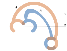
Figure 4: The sets $A$ and $B$ used in Remark 4.8.

Indeed, Figure 4 shows an example of a topological space $X=A\cup B$ on which, taking $\varphi$ equal to the height function and $u,v\in\mathbb{R}$ as displayed, it holds that $\mbox{\rm{rank}}\ker\alpha_{v}=\mbox{\rm{rank}}\ker\alpha_{v,u}\neq 0$, but $\mbox{\rm{rank}}\ker\alpha>0$, making the sequence (50) not exact. To see this, we note that the equalities (47) and (48) imply $\mbox{\rm{rank}}\ker\alpha_{v}=\mbox{\rm{rank}}\ker\alpha_{v,u}=1$.

As far as the homomorphism $\alpha$ is concerned, let us consider the homology sequence of the pair $(X_{v},X_{u})$

$$\begin{array}[]{ccccccccccc}\cdots&{\rightarrow}&\check{H}_{2}(X_{v},X_{u})&\stackrel{{\scriptstyle h}}{{\rightarrow}}&\check{H}_{1}(X_{u})&\stackrel{{\scriptstyle h_{1}}}{{\rightarrow}}&\check{H}_{1}(X_{v})&\stackrel{{\scriptstyle h^{\prime}_{1}}}{{\rightarrow}}&\check{H}_{1}(X_{v},X_{u})&{\rightarrow}&\cdots\end{array}$$

that is, the leftmost vertical line in diagram (46). In this instance, $\check{H}_{2}(X_{v},X_{u})=0$, so it follows that $h_{1}$ is injective. Now, recalling that, by Proposition 4.4, $\mbox{\rm{im\,}}\!\Delta\subseteq\ker\alpha$, where $\Delta=\Delta_{v|\mbox{\rm{im\,}}\!h_{1}}$, the triviality of $\check{H}_{1}(A_{v})\oplus\check{H}_{1}(B_{v})$, implies that $\Delta_{v}$ is surjective. So, since $\mbox{\rm{rank}}\check{H}_{1}(X_{u})=1$, it follows that $\mbox{\rm{rank}}\mbox{\rm{im\,}}\!\Delta=1$, and hence $\ker\alpha=1$ because $\ker\alpha\subseteq\ker\alpha_{v}$.

As shown in the proof of Proposition 4.7, it holds that $\ell_{(X,\varphi)}(u,v)=\ell_{(A,\varphi_{|A})}(u,v)+\ell_{(B,\varphi_{|B})}(u,v)-\mbox{\rm{rank}}\ker\beta$ for every $(u,v)\in\Delta^{+}$ (see equality (4.1)). So, as an immediate consequence, we observe that

Remark 4.9.

For every $(u,v)\in\Delta^{+}$, it holds that $\ell_{(X,\varphi)}(u,v)\leq\ell_{(A,\varphi_{|A})}(u,v)+\ell_{(B,\varphi_{|B})}(u,v)$.

4.2 Examples

In this section, we give two examples illustrating the previous results.

In both these examples, we consider a “double open-end wrench” shape $A$, partially occluded by another shape $B$, resulting in different shapes $X=A\cup B\subset\mathbb{R}^{2}$. The size functions $\ell_{(A,\varphi_{|A})}$, $\ell_{(B,\varphi_{|B})}$, $\ell_{(A\cap B,\varphi_{|A\cap B})}$, $\ell_{(X,\varphi)}$ are computed taking $\varphi:X\rightarrow\mathbb{R}$, $\varphi(P)=-\|P-H\|$, with $H$ a fixed point in $\mathbb{R}^{2}$.

\psfrag{A}{$A$}\psfrag{B}{$B$}\psfrag{AuB}{$A\cup B$}\psfrag{AnB}{$A\cap B$}\psfrag{AnB}{$A\cap B$}\psfrag{u}{$u$}\psfrag{v}{$v$}\psfrag{0}{$0$}\psfrag{1}{$1$}\psfrag{2}{$2$}\psfrag{3}{$3$}\psfrag{4}{$4$}\psfrag{-a}{$-a$}\psfrag{-b}{$-b$}\psfrag{-c}{$-c$}\psfrag{-d}{$-d$}\psfrag{a}{$a$}\psfrag{b}{$b$}\psfrag{c}{$c$}\psfrag{d}{$d$}\psfrag{H}{$H$}\psfrag{D+}{$\Delta^{+}$}\psfrag{la}{$\ell_{(A,\varphi_{|A})}$}\psfrag{lb}{$\ell_{(B,\varphi_{|B})}$}\psfrag{laub}{$\ell_{(A\cup B,\varphi)}$}\psfrag{lanb}{$\ell_{(A\cap B,\varphi_{|A\cap B})}$}\includegraphics[height=119.50148pt]{boneXOccPink.eps}

\psfrag{A}{$A$}\psfrag{B}{$B$}\psfrag{AuB}{$A\cup B$}\psfrag{AnB}{$A\cap B$}\psfrag{AnB}{$A\cap B$}\psfrag{u}{$u$}\psfrag{v}{$v$}\psfrag{0}{$0$}\psfrag{1}{$1$}\psfrag{2}{$2$}\psfrag{3}{$3$}\psfrag{4}{$4$}\psfrag{-a}{$-a$}\psfrag{-b}{$-b$}\psfrag{-c}{$-c$}\psfrag{-d}{$-d$}\psfrag{a}{$a$}\psfrag{b}{$b$}\psfrag{c}{$c$}\psfrag{d}{$d$}\psfrag{H}{$H$}\psfrag{D+}{$\Delta^{+}$}\psfrag{la}{$\ell_{(A,\varphi_{|A})}$}\psfrag{lb}{$\ell_{(B,\varphi_{|B})}$}\psfrag{laub}{$\ell_{(A\cup B,\varphi)}$}\psfrag{lanb}{$\ell_{(A\cap B,\varphi_{|A\cap B})}$}\includegraphics[height=113.81102pt]{osso_occluso1sf.eps}

$(a)$

$(b)$

\psfrag{A}{$A$}\psfrag{B}{$B$}\psfrag{AuB}{$A\cup B$}\psfrag{AnB}{$A\cap B$}\psfrag{AnB}{$A\cap B$}\psfrag{u}{$u$}\psfrag{v}{$v$}\psfrag{0}{$0$}\psfrag{1}{$1$}\psfrag{2}{$2$}\psfrag{3}{$3$}\psfrag{4}{$4$}\psfrag{-a}{$-a$}\psfrag{-b}{$-b$}\psfrag{-c}{$-c$}\psfrag{-d}{$-d$}\psfrag{a}{$a$}\psfrag{b}{$b$}\psfrag{c}{$c$}\psfrag{d}{$d$}\psfrag{H}{$H$}\psfrag{D+}{$\Delta^{+}$}\psfrag{la}{$\ell_{(A,\varphi_{|A})}$}\psfrag{lb}{$\ell_{(B,\varphi_{|B})}$}\psfrag{laub}{$\ell_{(A\cup B,\varphi)}$}\psfrag{lanb}{$\ell_{(A\cap B,\varphi_{|A\cap B})}$}\includegraphics[height=113.81102pt]{ossosf.eps}	\psfrag{A}{$A$}\psfrag{B}{$B$}\psfrag{AuB}{$A\cup B$}\psfrag{AnB}{$A\cap B$}\psfrag{AnB}{$A\cap B$}\psfrag{u}{$u$}\psfrag{v}{$v$}\psfrag{0}{$0$}\psfrag{1}{$1$}\psfrag{2}{$2$}\psfrag{3}{$3$}\psfrag{4}{$4$}\psfrag{-a}{$-a$}\psfrag{-b}{$-b$}\psfrag{-c}{$-c$}\psfrag{-d}{$-d$}\psfrag{a}{$a$}\psfrag{b}{$b$}\psfrag{c}{$c$}\psfrag{d}{$d$}\psfrag{H}{$H$}\psfrag{D+}{$\Delta^{+}$}\psfrag{la}{$\ell_{(A,\varphi_{|A})}$}\psfrag{lb}{$\ell_{(B,\varphi_{|B})}$}\psfrag{laub}{$\ell_{(A\cup B,\varphi)}$}\psfrag{lanb}{$\ell_{(A\cap B,\varphi_{|A\cap B})}$}\includegraphics[height=113.81102pt]{osso_occlusionesf1.eps}	\psfrag{A}{$A$}\psfrag{B}{$B$}\psfrag{AuB}{$A\cup B$}\psfrag{AnB}{$A\cap B$}\psfrag{AnB}{$A\cap B$}\psfrag{u}{$u$}\psfrag{v}{$v$}\psfrag{0}{$0$}\psfrag{1}{$1$}\psfrag{2}{$2$}\psfrag{3}{$3$}\psfrag{4}{$4$}\psfrag{-a}{$-a$}\psfrag{-b}{$-b$}\psfrag{-c}{$-c$}\psfrag{-d}{$-d$}\psfrag{a}{$a$}\psfrag{b}{$b$}\psfrag{c}{$c$}\psfrag{d}{$d$}\psfrag{H}{$H$}\psfrag{D+}{$\Delta^{+}$}\psfrag{la}{$\ell_{(A,\varphi_{|A})}$}\psfrag{lb}{$\ell_{(B,\varphi_{|B})}$}\psfrag{laub}{$\ell_{(A\cup B,\varphi)}$}\psfrag{lanb}{$\ell_{(A\cap B,\varphi_{|A\cap B})}$}\includegraphics[height=113.81102pt]{osso_intersezsf1.eps}
$(c)$	$(d)$	$(e)$

Figure 5: In $(a)$ a “double open-end wrench” shape $A$ is occluded by another shape $B$. In $(b)$, $(c)$, $(d)$ and $(e)$ we show the size functions of $(A\cup B,\varphi)$, $(A,\varphi_{|A})$, $(B,\varphi_{|B})$, and $(A\cap B,\varphi_{|A\cap B})$, respectively, computed taking $\varphi:X\rightarrow\mathbb{R}$, $\varphi(P)=-\|P-H\|$. In this example the relation $\ell_{(X,\varphi)}=\ell_{(A,\varphi_{|A})}+\ell_{(B,\varphi_{|B})}-\ell_{(A\cap B,\varphi_{|A\cap B})}$ of Corollary 4.6 holds everywhere in $\Delta^{+}$.

In the first example, shown in Figure 5, the relation $\ell_{(X,\varphi)}(u,v)=\ell_{(A,\varphi_{|A})}(u,v)+\ell_{(B,\varphi_{|B})}(u,v)-\ell_{(A\cap B,\varphi_{|A\cap B})}(u,v)$, given in Corollary 4.6, holds for every $(u,v)\in\Delta^{+}$.

\psfrag{A}{$A$}\psfrag{B}{$B$}\psfrag{AuB}{$A\cup B$}\psfrag{AnB}{$A\cap B$}\psfrag{u}{$u$}\psfrag{v}{$v$}\psfrag{0}{$0$}\psfrag{1}{$1$}\psfrag{2}{$2$}\psfrag{3}{$3$}\psfrag{4}{$4$}\psfrag{-a}{$-a$}\psfrag{-b}{$-b$}\psfrag{-c}{$-c$}\psfrag{-d}{$-d$}\psfrag{a}{$a$}\psfrag{b}{$b$}\psfrag{c}{$c$}\psfrag{d}{$d$}\psfrag{H}{$H$}\psfrag{D+}{$\Delta^{+}$}\psfrag{la}{$\ell_{(A,\varphi_{|A})}$}\psfrag{lb}{$\ell_{(B,\varphi_{|B})}$}\psfrag{laub}{$\ell_{(A\cup B,\varphi)}$}\psfrag{lanb}{$\ell_{(A\cap B,\varphi_{|A\cap B})}$}\includegraphics[height=119.50148pt]{boneXOccHolePink.eps}	\psfrag{A}{$A$}\psfrag{B}{$B$}\psfrag{AuB}{$A\cup B$}\psfrag{AnB}{$A\cap B$}\psfrag{u}{$u$}\psfrag{v}{$v$}\psfrag{0}{$0$}\psfrag{1}{$1$}\psfrag{2}{$2$}\psfrag{3}{$3$}\psfrag{4}{$4$}\psfrag{-a}{$-a$}\psfrag{-b}{$-b$}\psfrag{-c}{$-c$}\psfrag{-d}{$-d$}\psfrag{a}{$a$}\psfrag{b}{$b$}\psfrag{c}{$c$}\psfrag{d}{$d$}\psfrag{H}{$H$}\psfrag{D+}{$\Delta^{+}$}\psfrag{la}{$\ell_{(A,\varphi_{|A})}$}\psfrag{lb}{$\ell_{(B,\varphi_{|B})}$}\psfrag{laub}{$\ell_{(A\cup B,\varphi)}$}\psfrag{lanb}{$\ell_{(A\cap B,\varphi_{|A\cap B})}$}\includegraphics[height=113.81102pt]{osso_occluso4sf.eps}	\psfrag{A}{$A$}\psfrag{B}{$B$}\psfrag{AuB}{$A\cup B$}\psfrag{AnB}{$A\cap B$}\psfrag{u}{$u$}\psfrag{v}{$v$}\psfrag{0}{$0$}\psfrag{1}{$1$}\psfrag{2}{$2$}\psfrag{3}{$3$}\psfrag{4}{$4$}\psfrag{-a}{$-a$}\psfrag{-b}{$-b$}\psfrag{-c}{$-c$}\psfrag{-d}{$-d$}\psfrag{a}{$a$}\psfrag{b}{$b$}\psfrag{c}{$c$}\psfrag{d}{$d$}\psfrag{H}{$H$}\psfrag{D+}{$\Delta^{+}$}\psfrag{la}{$\ell_{(A,\varphi_{|A})}$}\psfrag{lb}{$\ell_{(B,\varphi_{|B})}$}\psfrag{laub}{$\ell_{(A\cup B,\varphi)}$}\psfrag{lanb}{$\ell_{(A\cap B,\varphi_{|A\cap B})}$}\includegraphics[height=113.81102pt]{osso_occluso4sfspiega.eps}
$(a)$	$(b)$	$(c)$

\psfrag{A}{$A$}\psfrag{B}{$B$}\psfrag{AuB}{$A\cup B$}\psfrag{AnB}{$A\cap B$}\psfrag{u}{$u$}\psfrag{v}{$v$}\psfrag{0}{$0$}\psfrag{1}{$1$}\psfrag{2}{$2$}\psfrag{3}{$3$}\psfrag{4}{$4$}\psfrag{-a}{$-a$}\psfrag{-b}{$-b$}\psfrag{-c}{$-c$}\psfrag{-d}{$-d$}\psfrag{a}{$a$}\psfrag{b}{$b$}\psfrag{c}{$c$}\psfrag{d}{$d$}\psfrag{H}{$H$}\psfrag{D+}{$\Delta^{+}$}\psfrag{la}{$\ell_{(A,\varphi_{|A})}$}\psfrag{lb}{$\ell_{(B,\varphi_{|B})}$}\psfrag{laub}{$\ell_{(A\cup B,\varphi)}$}\psfrag{lanb}{$\ell_{(A\cap B,\varphi_{|A\cap B})}$}\includegraphics[height=113.81102pt]{osso3sf.eps}	\psfrag{A}{$A$}\psfrag{B}{$B$}\psfrag{AuB}{$A\cup B$}\psfrag{AnB}{$A\cap B$}\psfrag{u}{$u$}\psfrag{v}{$v$}\psfrag{0}{$0$}\psfrag{1}{$1$}\psfrag{2}{$2$}\psfrag{3}{$3$}\psfrag{4}{$4$}\psfrag{-a}{$-a$}\psfrag{-b}{$-b$}\psfrag{-c}{$-c$}\psfrag{-d}{$-d$}\psfrag{a}{$a$}\psfrag{b}{$b$}\psfrag{c}{$c$}\psfrag{d}{$d$}\psfrag{H}{$H$}\psfrag{D+}{$\Delta^{+}$}\psfrag{la}{$\ell_{(A,\varphi_{|A})}$}\psfrag{lb}{$\ell_{(B,\varphi_{|B})}$}\psfrag{laub}{$\ell_{(A\cup B,\varphi)}$}\psfrag{lanb}{$\ell_{(A\cap B,\varphi_{|A\cap B})}$}\includegraphics[height=113.81102pt]{osso_occlusionesf3.eps}	\psfrag{A}{$A$}\psfrag{B}{$B$}\psfrag{AuB}{$A\cup B$}\psfrag{AnB}{$A\cap B$}\psfrag{u}{$u$}\psfrag{v}{$v$}\psfrag{0}{$0$}\psfrag{1}{$1$}\psfrag{2}{$2$}\psfrag{3}{$3$}\psfrag{4}{$4$}\psfrag{-a}{$-a$}\psfrag{-b}{$-b$}\psfrag{-c}{$-c$}\psfrag{-d}{$-d$}\psfrag{a}{$a$}\psfrag{b}{$b$}\psfrag{c}{$c$}\psfrag{d}{$d$}\psfrag{H}{$H$}\psfrag{D+}{$\Delta^{+}$}\psfrag{la}{$\ell_{(A,\varphi_{|A})}$}\psfrag{lb}{$\ell_{(B,\varphi_{|B})}$}\psfrag{laub}{$\ell_{(A\cup B,\varphi)}$}\psfrag{lanb}{$\ell_{(A\cap B,\varphi_{|A\cap B})}$}\includegraphics[height=113.81102pt]{osso_intersezsf4.eps}
$(d)$	$(e)$	$(f)$

Figure 6: In $(a)$ the same “double open-end wrench” shape $A$ as in Figure 5 is considered together with a different occluding shape $B$. In $(b)$, $(d)$, $(e)$, $(f)$ we display the size functions of $(A\cup B,\varphi)$, $(A,\varphi_{|A})$, $(B,\varphi_{|B})$, and $(A\cap B,\varphi_{|A\cap B})$, respectively, computed taking $\varphi:X\rightarrow\mathbb{R}$, $\varphi(P)=-\|P-H\|$. In this case the relation $\ell_{(X,\varphi)}=\ell_{(A,\varphi_{|A})}+\ell_{(B,\varphi_{|B})}-\ell_{(A\cap B,\varphi_{|A\cap B})}$ of Corollary 4.6 does not hold everywhere in $\Delta^{+}$. In $(c)$ we underline the regions of $\Delta^{+}$ where the equality is not valid by coloring them.

In the second example, shown in Figure 6, a deformation of occluding shape $B$ in Figure 5 makes the relation given in Corollary 4.6 not valid everywhere in $\Delta^{+}$.

More precisely, the condition $\mbox{\rm{rank}}\ker\alpha_{v}=\mbox{\rm{rank}}\ker\alpha_{v,u}=1$ holds for every $(u,v)\in\Delta^{+}$, with $-a\leq u<-b$ and $-c\leq v$, whereas the condition $\mbox{\rm{rank}}\ker\alpha_{v}=\mbox{\rm{rank}}\ker\alpha_{v,u}=0$ holds for every $(u,v)\in\Delta^{+}$ with $u<-a$, for every $(u,v)\in\Delta^{+}$ with $-a\leq u<v<-b$, and for every $(u,v)\in\Delta^{+}$ with $-b\leq u<v<-c$. Therefore, in these regions, $\ell_{(X,\varphi)}(u,v)=\ell_{(A,\varphi_{|A})}(u,v)+\ell_{(B,\varphi_{|B})}(u,v)-\ell_{(A\cap B,\varphi_{|A\cap B})}(u,v)$. In the remaining regions of $\Delta^{+}$, this relation does not hold. In particular, for every $(u,v)\in\Delta^{+}$ with $-a\leq u<-b$ and $-b\leq v<-c$ we have $\mbox{\rm{rank}}\ker\alpha_{v}=0$ and $\mbox{\rm{rank}}\ker\alpha_{v,u}=1$, yielding $\ell_{(X,\varphi)}(u,v)<\ell_{(A,\varphi_{|A})}(u,v)+\ell_{(B,\varphi_{|B})}(u,v)-\ell_{(A\cap B,\varphi_{|A\cap B})}(u,v)$, while for every $(u,v)\in\Delta^{+}$ with $-b\leq u$ and $-c\leq v$ we have $\mbox{\rm{rank}}\ker\alpha_{v}=1$ and $\mbox{\rm{rank}}\ker\alpha_{v,u}=0$, yielding $\ell_{(X,\varphi)}(u,v)>\ell_{(A,\varphi_{|A})}(u,v)+\ell_{(B,\varphi_{|B})}(u,v)-\ell_{(A\cap B,\varphi_{|A\cap B})}(u,v)$. To simplify the visualization of the regions of $\Delta^{+}$ in which the equality holds, the reader can refer to Figure 6 $(c)$, where $\ell_{(X,\varphi)}$ is displayed using white for points $(u,v)\in\Delta^{+}$ that verify $\ell_{(X,\varphi)}(u,v)=\ell_{(A,\varphi_{|A})}(u,v)+\ell_{(B,\varphi_{|B})}(u,v)-\ell_{(A\cap B,\varphi_{|A\cap B})}(u,v)$ and red for the other ones.

4.3 Conditions for the exactness of $0\rightarrow\check{H}_{0}^{u,v}(A\cap B)\rightarrow\check{H}_{0}^{u,v}(A)\oplus\check{H}_{0}^{u,v}(B)\rightarrow\check{H}_{0}^{u,v}(X)\rightarrow 0$

In this section we look for sufficient conditions in order that $\alpha_{v}$ and $\alpha_{v,u}$ are injective, so that the sequence

$$\begin{array}[]{ccccccc}0&{\rightarrow}&\check{H}_{0}^{u,v}(A\cap B)&\stackrel{{\scriptstyle\alpha}}{{\rightarrow}}&\check{H}_{0}^{u,v}(A)\oplus\check{H}_{0}^{u,v}(B)&\stackrel{{\scriptstyle\beta}}{{\rightarrow}}&\check{H}_{0}^{u,v}(X)\rightarrow 0\end{array}$$

is exact (cf. Proposition 4.7), and the relation $\ell_{(X,\varphi)}(u,v)=\ell_{(A,\varphi_{|A})}(u,v)+\ell_{(B,\varphi_{|B})}(u,v)-\ell_{(A\cap B,\varphi_{|A\cap B})}(u,v)$ of Corollary 4.6 is satisfied.

The reason for identifying these conditions lies in the fact that they can be used as a guidance in choosing the most appropriate measuring function in order to study the shape of a partially occluded object.

The first condition we exhibit (Theorem 4.11), relates the exactness of the above sequence to the values taken by the size function $\ell_{(A\cap B,\varphi_{|A\cap B})}$. Roughly speaking, it indicates that the fewer the number of cornerpoints in the size function of $A\cap B$, the larger the region of $\Delta^{+}$ where the above sequence is necessarily exact. We underline that this is only a sufficient condition, as the examples in Section 4.2 easily show.

The sketch of proof is the following. We begin by showing that the surjectivity of $f_{0}$ is a sufficient condition, ensuring that $\alpha_{v,u}$ is injective. Then we note that, for points $(u,v)\in\Delta^{+}$ where the size function of $A\cap B$ has no cornerpoints in the upper right region $\{(u^{\prime},v^{\prime})\in\Delta^{+}:\ u\leq u^{\prime}\leq v,v^{\prime}>v\}$, $f_{0}$ is necessarily surjective. So we obtain a condition on $\ell_{(A\cap B,\varphi_{|A\cap B})}(u,v)$ such that $\alpha_{v,u}$ is injective. Finally, showing that if $\ell_{(A\cap B,\varphi_{|A\cap B})}(u,v)\leq 1$, then $\alpha_{v}$ is injective, we prove the claim of Theorem 4.11.

Lemma 4.10.

Let $\alpha={\alpha_{v}}_{|\mbox{\rm{im\,}}\!f_{0}}$ and $\beta={\beta_{v}}_{|\mbox{\rm{im\,}}\!g_{0}}$. If $f_{0}$ is surjective, then $\mbox{\rm{im\,}}\!\alpha=\ker\beta$ and $\alpha_{v,u}=0$.

Proof.

By Proposition 4.4(ii), $\mbox{\rm{im\,}}\!\alpha\subseteq\ker\beta$, so we need to prove that $\ker\beta\subseteq\mbox{\rm{im\,}}\!\alpha$. Let $c\in\ker\beta\subseteq\ker\beta_{v}$. Since $\mbox{\rm{im\,}}\!\alpha_{v}=\ker\beta_{v}$, there exists $d\in\check{H}_{0}((A\cap B)_{v})$ such that $\alpha_{v}(d)=c$. By hypothesis, $f_{0}$ is surjective, so $\check{H}_{0}((A\cap B)_{v})=\mbox{\rm{im\,}}\!f_{0}$. Hence $d\in\mbox{\rm{im\,}}\!f_{0}$, implying $\alpha(d)=c$. Thus, $c\in\mbox{\rm{im\,}}\!\alpha$, and hence $\mbox{\rm{im\,}}\!\alpha=\ker\beta$.

Let us now show that $\alpha_{v,u}$ is trivial. By observing diagram (46), we see that $f_{0}$ is surjective if and only if $f_{0}^{\prime}$ is trivial. Since $f_{0}^{\prime}$ is surjective, it holds that $f_{0}$ is surjective if and only if $\check{H}_{0}((A\cap B)_{v},(A\cap B)_{u})=0$. Therefore, if $f_{0}$ is surjective, then $\alpha_{v,u}=0$. ∎

Theorem 4.11.

Let $(u,v)\in\Delta^{+}$. If $\ell_{(A\cap B,\varphi_{|A\cap B})}(u,v^{\prime})=\ell_{(A\cap B,\varphi_{|A\cap B})}(v,v^{\prime})\leq 1$, for every $(v,v^{\prime})\in\Delta^{+}$, then $\ker\alpha_{v}=\ker\alpha_{v,u}=0$.

Proof.

From $\ell_{(A\cap B,\varphi_{|A\cap B})}(u,v^{\prime})=\ell_{(A\cap B,\varphi_{|A\cap B})}(v,v^{\prime})$, applying Proposition 3.12 with $A\cap B$ in place of $X$ and $f_{0}$ in place of $\iota_{0}^{u,v}$, it follows that $f_{0}$ is surjective. Hence, by Lemma 4.10, we have that $\alpha_{v,u}$ is trivial.

Let us now prove that $\alpha_{v}$ is injective. From the assumption $\ell_{(A\cap B,\varphi_{|A\cap B})}(v,v^{\prime})\leq 1$, for every $(v,v^{\prime})\in\Delta^{+}$, we deduce that either $(A\cap B)_{v}$ is empty or $(A\cap B)_{v}$ is non-empty and connected. If $(A\cap B)_{v}$ is empty, then $\check{H}_{0}((A\cap B)_{v})$ is trivial and the claim is proved. Let us consider the case when $(A\cap B)_{v}$ is non-empty and connected. Let $z_{0}=\{z_{0}({\mathcal{U}}_{(A\cap B)_{v}})\}\in\check{H}_{0}((A\cap B)_{v})$. If $z_{0}\in\ker\alpha_{v}=\mbox{\rm{im\,}}\!\Delta_{v}$, for each $z_{0}({\mathcal{U}}_{(A\cap B)_{v}})\in H_{0}({\mathcal{U}}_{(A\cap B)_{v}})$ there is a $1$-chain $c_{1}({\mathcal{U}}_{A_{v}})$ on $A_{v}$ and a $1$-chain $c_{1}({\mathcal{U}}_{B_{v}})$ on $B_{v}$, such that the homology class of $\partial c_{1}({\mathcal{U}}_{A_{v}})=-\partial c_{1}({\mathcal{U}}_{B_{v}})$ is equal to $z_{0}({\mathcal{U}}_{(A\cap B)_{v}})$, up to homomorphisms induced by inclusion. We now show that $\partial c_{1}({\mathcal{U}}_{A_{v}})$ is a boundary on $(A\cap B)_{v}$. This will prove that $z_{0}({\mathcal{U}}_{(A\cap B)_{v}})$ is trivial, yielding the injectivity of $\alpha_{v}$. If $c_{1}({\mathcal{U}}_{A_{v}})=\sum_{i=1}^{n}a_{i}\cdot<U_{i}^{0},U_{i}^{1}>$, then $\partial c_{1}({\mathcal{U}}_{A_{v}})=\sum_{i=1}^{n}a_{i}\cdot U_{i}^{1}-\sum_{i=1}^{n}a_{i}\cdot U_{i}^{0}$. From $\partial c_{1}({\mathcal{U}}_{A_{v}})=-\partial c_{1}({\mathcal{U}}_{B_{v}})$, we deduce that, for $i=1,\ldots,n$, both $U_{i}^{0}$ and $U_{i}^{1}$ intersect $(A\cap B)_{v}$. By Proposition 3.3, the connectedness of $(A\cap B)_{v}$ implies that there is a simple chain on $(A\cap B)_{v}$ connecting $U_{i}^{0}$ and $U_{i}^{1}$, for $i=1,\ldots,n$. Therefore $\partial c_{1}({\mathcal{U}}_{A_{v}})$ is a boundary on $(A\cap B)_{v}$. ∎

We conclude by observing that other sufficient conditions exist, implying that both $\alpha_{v}$ and $\alpha_{v,u}$ are injective. An example is given by the following result.

Proposition 4.12.

If $\mbox{\rm{rank}}\check{H}_{1}(X_{v})=0$ and $\mbox{\rm{rank}}\check{H}_{0}(X_{u})=\ell_{(X,\varphi)}(u,v)$, then $\ker\alpha_{v}=\ker\alpha_{v,u}=0$.

Proof.

The condition $\mbox{\rm{rank}}\check{H}_{1}(X_{v})=0$ trivially implies $\ker\alpha_{v}=0$. On the other hand, it implies the injectivity of the homomorphism $h$ in the following exact sequence:

$$\begin{array}[]{ccccccccccc}\cdots&{\rightarrow}&\check{H}_{1}(X_{v})&\stackrel{{\scriptstyle h^{\prime}_{1}}}{{\rightarrow}}&\check{H}_{1}(X_{v},X_{u})&\stackrel{{\scriptstyle h}}{{\rightarrow}}&\check{H}_{0}(X_{u})&\stackrel{{\scriptstyle h_{0}}}{{\rightarrow}}&\check{H}_{0}(X_{v})&\stackrel{{\scriptstyle h^{\prime}_{0}}}{{\rightarrow}}&\check{H}_{0}(X_{v},X_{u})\rightarrow 0,\end{array}$$

which is the leftmost vertical sequence in diagram (46). Therefore, by the assumption $\mbox{\rm{rank}}\check{H}_{0}(X_{u})=\ell_{(X,\varphi)}(u,v)$, it follows that

$$\mbox{\rm{rank}}\check{H}_{1}(X_{v},X_{u})=\mbox{\rm{rank}}\mbox{\rm{im\,}}\!h=\mbox{\rm{rank}}\ker h_{0}=\mbox{\rm{rank}}\check{H}_{0}(X_{u})-\ell_{(X,\varphi)}(u,v)=0,$$

and, consequently, the triviality of $\ker\alpha_{v,u}$ has been proved. ∎

5 Partial matching of cornerpoints in size functions

As recalled in Section 2, in an earlier paper [19], it was shown that size functions can be concisely represented by collections of points, called cornerpoints, with multiplicities.

This representation by cornerpoints has the important property of being stable against shape continuous deformations. For this reason, in dealing with the shape comparison problem, via size functions, one actually compares the sets of cornerpoints using either the Hausdorff distance or the matching distance (see e.g. [8, 10, 11, 18]). The Hausdorff distance and the matching distance differ in that the former does not take into account the multiplicities of cornerpoints, while the latter does.

The aim of this section is to show what happens to cornerpoints in the presence of occlusions. We prove that each cornerpoint for the size function of an occluded shape $X$ is a cornerpoint for the size function of the original shape $A$, or the occluding shape $B$, or their intersection $A\cap B$, providing that one condition holds (Corollary 5.2). However, even when this condition is not verified, it holds that the coordinates of cornerpoints of $\ell_{(X,\varphi)}$ are always related to the cornerpoints of $\ell_{(A,\varphi|_{A})}$ or $\ell_{(B,\varphi|_{B})}$ or $\ell_{(A\cap B,\varphi|_{A\cap B})}$ (Theorems 5.4 and 5.5).

We begin by proving a relation between multiplicities of points for the size functions associated with $X$, $A$ and $B$. Since cornerpoints are points with positive multiplicity (cf. Definitions 2.3 and 2.4), we obtain conditions for cornerpoints of the size functions of $A$ and $B$ to persist in $A\cup B$. This fact suggests that in size theory the partial matching of an occluded shape with the original shape can be translated into the partial matching of cornerpoints of the corresponding size functions. This intuition will be developed in the experimental Section 6.

In the next proposition we obtain a relation involving the multiplicities of points in the size functions associated with $X$, $A$ and $B$.

Proposition 5.1.

For every $p=(\overline{u},\overline{v})\in\Delta^{+}$, it holds that

$$\mu_{X}(p)-\mu_{A}(p)-\mu_{B}(p)+\mu_{A\cap B}(p)=\lim_{\epsilon\rightarrow 0^{+}}\left(\mbox{\rm{rank}}\ker\alpha_{\bar{v}-\epsilon,\bar{u}-\epsilon}-\mbox{\rm{rank}}\ker\alpha_{\bar{v}-\epsilon,\bar{u}+\epsilon}+\mbox{\rm{rank}}\ker\alpha_{\bar{v}+\epsilon,\bar{u}+\epsilon}-\mbox{\rm{rank}}\ker\alpha_{\bar{v}+\epsilon,\bar{u}-\epsilon}\right).$$

Proof.

Applying Theorem 4.5 four times with $(u,v)=(\overline{u}+\epsilon,\overline{v}-\epsilon)$, $(u,v)=(\overline{u}-\epsilon,\overline{v}-\epsilon)$, $(u,v)=(\overline{u}+\epsilon,\overline{v}+\epsilon)$, $(u,v)=(\overline{u}-\epsilon,\overline{v}+\epsilon)$, $\epsilon$ being a positive real number so small that $\overline{u}+\epsilon<\overline{v}-\epsilon$, we get

$$\ell_{(X,\varphi)}(\overline{u}+\epsilon,\overline{v}-\epsilon)-\ell_{(X,\varphi)}(\overline{u}-\epsilon,\overline{v}-\epsilon)-\ell_{(X,\varphi)}(\overline{u}+\epsilon,\overline{v}+\epsilon)+\ell_{(X,\varphi)}(\overline{u}-\epsilon,\overline{v}+\epsilon)$$

$$= \ell_{(A,\varphi_{|A})}(\overline{u}+\epsilon,\overline{v}-\epsilon)+\ell_{(B,\varphi_{|B})}(\overline{u}+\epsilon,\overline{v}-\epsilon)-\ell_{(A\cap B,\varphi_{|A\cap B})}(\overline{u}+\epsilon,\overline{v}-\epsilon)+\mbox{\rm{rank}}\ker\alpha_{\bar{v}-\epsilon}-\mbox{\rm{rank}}\ker\alpha_{\bar{v}-\epsilon,\bar{u}+\epsilon}$$

$$-\left(\ell_{(A,\varphi_{|A})}(\overline{u}-\epsilon,\overline{v}-\epsilon)+\ell_{(B,\varphi_{|B})}(\overline{u}-\epsilon,\overline{v}-\epsilon)-\ell_{(A\cap B,\varphi_{|A\cap B})}(\overline{u}-\epsilon,\overline{v}-\epsilon)+\mbox{\rm{rank}}\ker\alpha_{\bar{v}-\epsilon}-\mbox{\rm{rank}}\ker\alpha_{\bar{v}-\epsilon,\bar{u}-\epsilon}\right)$$

$$-\left(\ell_{(A,\varphi_{|A})}(\overline{u}+\epsilon,\overline{v}+\epsilon)+\ell_{(B,\varphi_{|B})}(\overline{u}+\epsilon,\overline{v}+\epsilon)-\ell_{(A\cap B,\varphi_{|A\cap B})}(\overline{u}+\epsilon,\overline{v}+\epsilon)+\mbox{\rm{rank}}\ker\alpha_{\bar{v}+\epsilon}-\mbox{\rm{rank}}\ker\alpha_{\bar{v}+\epsilon,\bar{u}+\epsilon}\right)$$

$$+\ell_{(A,\varphi_{|A})}(\overline{u}-\epsilon,\overline{v}+\epsilon)+\ell_{(B,\varphi_{|B})}(\overline{u}-\epsilon,\overline{v}+\epsilon)-\ell_{(A\cap B,\varphi_{|A\cap B})}(\overline{u}-\epsilon,\overline{v}+\epsilon)+\mbox{\rm{rank}}\ker\alpha_{\bar{v}+\epsilon}-\mbox{\rm{rank}}\ker\alpha_{\bar{v}+\epsilon,\bar{u}-\epsilon}$$

$$= \ell_{(A,\varphi)}(\overline{u}+\epsilon,\overline{v}-\epsilon)-\ell_{(A,\varphi)}(\overline{u}-\epsilon,\overline{v}-\epsilon)-\ell_{(A,\varphi)}(\overline{u}+\epsilon,\overline{v}+\epsilon)+\ell_{(A,\varphi)}(\overline{u}-\epsilon,\overline{v}+\epsilon)$$

$$+\ell_{(B,\varphi)}(\overline{u}+\epsilon,\overline{v}-\epsilon)-\ell_{(B,\varphi)}(\overline{u}-\epsilon,\overline{v}-\epsilon)-\ell_{(B,\varphi)}(\overline{u}+\epsilon,\overline{v}+\epsilon)+\ell_{(B,\varphi)}(\overline{u}-\epsilon,\overline{v}+\epsilon)$$

$$-\ell_{(A\cap B,\varphi)}(\overline{u}+\epsilon,\overline{v}-\epsilon)+\ell_{(A\cap B,\varphi)}(\overline{u}-\epsilon,\overline{v}-\epsilon)+\ell_{(A\cap B,\varphi)}(\overline{u}+\epsilon,\overline{v}+\epsilon)-\ell_{(A\cap B,\varphi)}(\overline{u}-\epsilon,\overline{v}+\epsilon)$$

$$+\mbox{\rm{rank}}\ker\alpha_{\bar{v}-\epsilon,\bar{u}-\epsilon}-\mbox{\rm{rank}}\ker\alpha_{\bar{v}-\epsilon,\bar{u}+\epsilon}+\mbox{\rm{rank}}\ker\alpha_{\bar{v}+\epsilon,\bar{u}+\epsilon}-\mbox{\rm{rank}}\ker\alpha_{\bar{v}+\epsilon,\bar{u}-\epsilon}.$$

Hence, by definition of multiplicity of a point of $\Delta^{+}$ (Definition 2.3), we have that

$$\lim_{\epsilon\rightarrow 0^{+}}\left(\mbox{\rm{rank}}\ker\alpha_{\bar{v}-\epsilon,\bar{u}-\epsilon}-\mbox{\rm{rank}}\ker\alpha_{\bar{v}-\epsilon,\bar{u}+\epsilon}+\mbox{\rm{rank}}\ker\alpha_{\bar{v}+\epsilon,\bar{u}+\epsilon}-\mbox{\rm{rank}}\ker\alpha_{\bar{v}+\epsilon,\bar{u}-\epsilon}\right)$$

$$= \lim_{\epsilon\rightarrow 0^{+}}\left(\ell_{(X,\varphi)}(\overline{u}+\epsilon,\overline{v}-\epsilon)-\ell_{(X,\varphi)}(\overline{u}-\epsilon,\overline{v}-\epsilon)-\ell_{(X,\varphi)}(\overline{u}+\epsilon,\overline{v}+\epsilon)+\ell_{(X,\varphi)}(\overline{u}-\epsilon,\overline{v}+\epsilon)\right)$$

$$-\lim_{\epsilon\rightarrow 0^{+}}\left(\ell_{(A,\varphi)}(\overline{u}+\epsilon,\overline{v}-\epsilon)-\ell_{(A,\varphi)}(\overline{u}-\epsilon,\overline{v}-\epsilon)-\ell_{(A,\varphi)}(\overline{u}+\epsilon,\overline{v}+\epsilon)+\ell_{(A,\varphi)}(\overline{u}-\epsilon,\overline{v}+\epsilon)\right)$$

$$-\lim_{\epsilon\rightarrow 0^{+}}\left(\ell_{(B,\varphi)}(\overline{u}+\epsilon,\overline{v}-\epsilon)-\ell_{(B,\varphi)}(\overline{u}-\epsilon,\overline{v}-\epsilon)-\ell_{(B,\varphi)}(\overline{u}+\epsilon,\overline{v}+\epsilon)+\ell_{(B,\varphi)}(\overline{u}-\epsilon,\overline{v}+\epsilon)\right)$$

$$+\lim_{\epsilon\rightarrow 0^{+}}\left(\ell_{(A\cap B,\varphi)}(\overline{u}+\epsilon,\overline{v}-\epsilon)-\ell_{(A\cap B,\varphi)}(\overline{u}-\epsilon,\overline{v}-\epsilon)-\ell_{(A\cap B,\varphi)}(\overline{u}+\epsilon,\overline{v}+\epsilon)+\ell_{(A\cap B,\varphi)}(\overline{u}-\epsilon,\overline{v}+\epsilon)\right)$$

$$= \mu_{X}(p)-\mu_{A}(p)-\mu_{B}(p)+\mu_{A\cap B}(p).$$

∎

Using the previous Proposition 5.1, we find a condition ensuring that proper cornerpoints for the size function of $X$ are also proper cornerpoints for the size function of $A$ or $B$.

Corollary 5.2.

Let $p=(\overline{u},\overline{v})$ be a proper cornerpoint for $\ell_{(X,\varphi)}$ and

$$\lim_{\epsilon\rightarrow 0^{+}}\left(\mbox{\rm{rank}}\ker\alpha_{\bar{v}-\epsilon,\bar{u}-\epsilon}-\mbox{\rm{rank}}\ker\alpha_{\bar{v}-\epsilon,\bar{u}+\epsilon}+\mbox{\rm{rank}}\ker\alpha_{\bar{v}+\epsilon,\bar{u}+\epsilon}-\mbox{\rm{rank}}\ker\alpha_{\bar{v}+\epsilon,\bar{u}-\epsilon}\right)\leq 0.$$

Then $p$ is a proper cornerpoint for either $\ell_{(A,\varphi|_{A})}$ or $\ell_{(B,\varphi|_{B})}$ or both.

Proof.

Let $\underset{\epsilon\rightarrow 0^{+}}{\lim}\left(\mbox{\rm{rank}}\ker\alpha_{\bar{v}-\epsilon,\bar{u}-\epsilon}-\mbox{\rm{rank}}\ker\alpha_{\bar{v}-\epsilon,\bar{u}+\epsilon}+\mbox{\rm{rank}}\ker\alpha_{\bar{v}+\epsilon,\bar{u}+\epsilon}\right.-\left.\mbox{\rm{rank}}\ker\alpha_{\bar{v}+\epsilon,\bar{u}-\epsilon}\right)\leq 0$. From Proposition 5.1, we deduce that $\mu_{X}(p)\leq\mu_{A}(p)+\mu_{B}(p)-\mu_{A\cap B}(p)$. Since $p$ is a cornerpoint for $\ell_{(X,\varphi)}$, it holds that $\mu_{X}(p)>0$. Since multiplicities are always non-negative, this easily implies that either $\mu_{A}(p)>0$ or $\mu_{B}(p)>0$ (or both), proving the statement. ∎

Remark 5.3.

If $p=(\overline{u},\overline{v})$ is a proper cornerpoint for $\ell_{(X,\varphi)}$ and $\ell_{(A\cap B),\varphi_{|A\cap B}}(\overline{v},v^{\prime})\leq 1$ for every $v^{\prime}>\overline{v}$, then it is a proper cornerpoint for either $\ell_{(A,\varphi|_{A})}$ or $\ell_{(B,\varphi|_{B})}$ or both.

This is easily seen by combining Lemma 4.10 with Proposition 3.12 so that, by the right-continuity of size functions and the fact that they are non-decreasing in the first variable, for a sufficiently small $\epsilon$ it holds that $\ker\alpha_{\bar{v}-\epsilon,\bar{u}-\epsilon}=0$, $\ker\alpha_{\bar{v}-\epsilon,\bar{u}+\epsilon}=0$, $\ker\alpha_{\bar{v}+\epsilon,\bar{u}+\epsilon}=0$, $\ker\alpha_{\bar{v}+\epsilon,\bar{u}-\epsilon}=0$.

The following two theorems state that the abscissas of the cornerpoints for $\ell_{(X,\varphi)}$ are abscissas of cornerpoints for $\ell_{(A,\varphi|_{A})}$ or $\ell_{(B,\varphi|_{B})}$ or $\ell_{(A\cap B,\varphi|_{A\cap B})}$; the ordinates of the cornerpoints for $\ell_{(X,\varphi)}$ are, in general, homological 0-critical values for $(A,\varphi_{|A})$ or $(B,\varphi_{|B})$ or $(A\cap B,\varphi_{|A\cap B})$, and, under restrictive conditions, abscissas or ordinates of cornerpoints for $\ell_{(A,\varphi|_{A})}$ or $\ell_{(B,\varphi|_{B})}$ or $\ell_{(A\cap B,\varphi|_{A\cap B})}$, respectively.

These facts can easily be seen in the examples illustrated in Figures 5-6. In particular, in Figure 6, the size function $\ell_{(X,\varphi)}$ presents the proper cornerpoint $(-a,-b)$, which is neither a cornerpoint for $\ell_{(A,\varphi|_{A})}$ nor $\ell_{(B,\varphi|_{B})}$ nor $\ell_{(A\cap B,\varphi|_{A\cap B})}$. Nevertheless, its abscissa $-a$ is the abscissa of all cornerpoints for $\ell_{(A,\varphi|_{A})}$, while its ordinate $-b$ is the abscissa of the cornerpoint at infinity for both $\ell_{(B,\varphi|_{B})}$ and $\ell_{(A\cap B,\varphi|_{A\cap B})}$.

Theorem 5.4.

If $p=(\overline{u},\overline{v})\in\Delta^{+}$ is a proper cornerpoint for $\ell_{(X,\varphi)}$, then there exists at least one proper cornerpoint for $\ell_{(A,\varphi|_{A})}$ or $\ell_{(B,\varphi|_{B})}$ or $\ell_{(A\cap B,\varphi|_{A\cap B})}$ having $\overline{u}$ as abscissa. Moreover, if $(\overline{u},\infty)\in\Delta^{*}$ is a cornerpoint at infinity for $\ell_{(X,\varphi)}$, then it is a cornerpoint at infinity for $\ell_{(A,\varphi|_{A})}$ or $\ell_{(B,\varphi|_{B})}$.

Proof.

As for the first assertion, we prove the contrapositive statement.

Let $\overline{u}\in\mathbb{R}$, and let us suppose that there are no proper cornerpoints for $\ell_{(A,\varphi|_{A})}$, $\ell_{(B,\varphi|_{B})}$ and $\ell_{(A\cap B,\varphi|_{A\cap B})}$ having $\overline{u}$ as abscissa. Then it follows that, for every $v>\overline{u}$:

$$\begin{array}[]{l}\underset{\epsilon\rightarrow 0^{+}}{\lim}\left(\ell_{(A\cap B,\varphi|_{A\cap B})}(\overline{u}+\epsilon,v)-\ell_{(A\cap B,\varphi|_{A\cap B})}(\overline{u}-\epsilon,v)\right)=0,\\ \underset{\epsilon\rightarrow 0^{+}}{\lim}\left(\ell_{(A,\varphi|_{A})}(\overline{u}+\epsilon,v)-\ell_{(A,\varphi|_{A})}(\overline{u}-\epsilon,v)\right)=0,\\ \underset{\epsilon\rightarrow 0^{+}}{\lim}\left(\ell_{(B,\varphi|_{B})}(\overline{u}+\epsilon,v)-\ell_{(B,\varphi|_{B})}(\overline{u}-\epsilon,v)\right)=0.\end{array}$$

Indeed, if there exists $v>\overline{u}$, such that

$$\underset{\epsilon\rightarrow 0^{+}}{\lim}\left(\ell_{(A\cap B,\varphi|_{A\cap B})}(\overline{u}+\epsilon,v)-\ell_{(A\cap B,\varphi|_{A\cap B})}(\overline{u}-\epsilon,v)\right)\neq 0,$$

then $\overline{u}$ is a discontinuity point for $\ell_{(A\cap B,\varphi|_{A\cap B})}(\cdot,v)$, implying the presence of at least one proper cornerpoint having $\overline{u}$ as abscissa ([19], Lemma 3). Analogously for $\ell_{(A,\varphi|_{A})}$ and $\ell_{(B,\varphi|_{B})}$.

Moreover, since size functions are natural valued functions and are non-decreasing in the first variable, for every $v>\overline{u}$, there exists $\overline{\epsilon}>0$ small enough such that $v-\overline{\epsilon}>\overline{u}+\overline{\epsilon}$, and

$$0=\underset{\epsilon\rightarrow 0^{+}}{\lim}\left(\ell_{(A\cap B,\varphi|_{A\cap B})}(\overline{u}+\epsilon,v)-\ell_{(A\cap B,\varphi|_{A\cap B})}(\overline{u}-\epsilon,v)\right)=\ell_{(A\cap B,\varphi|_{A\cap B})}(\overline{u}+\overline{\epsilon},v)-\ell_{(A\cap B,\varphi|_{A\cap B})}(\overline{u}-\overline{\epsilon},v).$$

So, for every $\eta<\overline{\epsilon}$, we have $\ell_{(A\cap B,\varphi|_{A\cap B})}(\overline{u}+\eta,v)=\ell_{(A\cap B,\varphi|_{A\cap B})}(\overline{u}-\eta,v)$. This is equivalent to saying that $\mbox{\rm{rank}}\check{H}_{0}((A\cap B)_{v})-\mbox{\rm{rank}}\check{H}_{0}((A\cap B)_{v},(A\cap B)_{\overline{u}+\eta})=\mbox{\rm{rank}}\check{H}_{0}((A\cap B)_{v})-\mbox{\rm{rank}}\check{H}_{0}((A\cap B)_{v},(A\cap B)_{\overline{u}-\eta})$, that is, $\mbox{\rm{rank}}\check{H}_{0}((A\cap B)_{v},(A\cap B)_{\overline{u}+\eta})=\mbox{\rm{rank}}\check{H}_{0}((A\cap B)_{v},(A\cap B)_{\overline{u}-\eta}).$ Thus, in a similar way, for $\ell_{(A,\varphi|_{A})}$ and $\ell_{(B,\varphi|_{B})}$, we obtain $\mbox{\rm{rank}}\check{H}_{0}(A_{v},A_{\overline{u}+\eta})=\mbox{\rm{rank}}\check{H}_{0}(A_{v},A_{\overline{u}-\eta})$ and $\mbox{\rm{rank}}\check{H}_{0}(B_{v},B_{\overline{u}+\eta})=\mbox{\rm{rank}}\check{H}_{0}(B_{v},B_{\overline{u}-\eta}).$ Now, let us consider the following diagram:

where the homomorphisms $j_{1}$ and $j_{2}$ are induced by inclusions. Since they are surjective and their respective domain and codomain have the same rank, we deduce that $j_{1}$ and $j_{2}$ are isomorphisms. So, we obtain that $\ker\alpha_{v-\eta,\overline{u}-\eta}\simeq\ker\alpha_{v-\eta,\overline{u}+\eta}.$

Analogously, from the diagram

we can deduce that $\ker\alpha_{v+\eta,\overline{u}-\eta}\simeq\ker\alpha_{v+\eta,\overline{u}+\eta}$. Thus, since $\eta$ can be chosen arbitrarily small, it holds that

$$\begin{array}[]{l}\underset{\eta\rightarrow 0^{+}}{\lim}(\ker\alpha_{v-\eta,\overline{u}-\eta}-\ker\alpha_{v-\eta,\overline{u}+\eta})=0,\\ \underset{\eta\rightarrow 0^{+}}{\lim}(\ker\alpha_{v+\eta,\overline{u}-\eta}-\ker\alpha_{v+\eta,\overline{u}+\eta})=0.\end{array}$$

Therefore, applying Proposition 5.1, it follows that

$$\mu_{X}(p)-\mu_{A}(p)-\mu_{B}(p)+\mu_{A\cap B}(p)=0$$

and, in particular, by the hypothesis that $p=(\overline{u},v)$ is not a proper cornerpoint for $\ell_{(A\cap B,\varphi|_{A\cap B})}$, or $\ell_{(A,\varphi|_{A})}$, or $\ell_{(B,\varphi|_{B})}$, for any $v>\overline{u}$, it holds that $\mu_{X}(p)=0.$

In the case of cornerpoints at infinity, we observe that, if $(\overline{u},\infty)$ is a cornerpoint at infinity for $\ell_{(X,\varphi)}$, then $\overline{u}=\underset{p\in C}{\min}\varphi(p)$, for at least one connected component $C$ of $X$ ([19], Prop. 9). Furthermore, since $X=A\cup B$, it follows that $\overline{u}=\underset{p\in C\cap A}{\min}\varphi_{|A}(p)$ or $\overline{u}=\underset{p\in C\cap B}{\min}\varphi_{|B}(p)$, from which (by [19], Prop. 9), $(\overline{u},\infty)$ is shown to be a cornerpoint at infinity for $\ell_{(A,\varphi|_{A})}$ or $\ell_{(B,\varphi|_{B})}$. ∎

Theorem 5.5.

If $p=(\overline{u},\overline{v})\in\Delta^{+}$ is a proper cornerpoint for $\ell_{(X,\varphi)}$, then $\overline{v}$ is a homological 0-critical value for $(A,\varphi_{|A})$ or $(B,\varphi_{|B})$ or $(A\cap B,\varphi_{|A\cap B})$. Furthermore, if there exists at most a finite number of homological 0-critical values for $(A,\varphi_{|A})$, $(B,\varphi_{|B})$, and $(A\cap B,\varphi_{|A\cap B})$, then $\overline{v}$ is the abscissa of a cornerpoint (proper or at infinity) or the ordinate of a proper cornerpoint for $\ell_{(A,\varphi|_{A})}$ or $\ell_{(B,\varphi|_{B})}$ or $\ell_{(A\cap B,\varphi|_{A\cap B})}$.

Proof.

Regarding the first assertion, we prove the contrapositive statement.

Let $\overline{v}\in\mathbb{R}$, and let us suppose that $\overline{v}$ is not a homological 0-critical value for the size pairs $(A,\varphi_{|A})$, $(B,\varphi_{|B})$ and $(A\cap B,\varphi_{|A\cap B})$. Then, by Definition 3.8, for every $\overline{\epsilon}>0$, there exists $\epsilon$ with $0<\epsilon<\overline{\epsilon}$, such that the vertical homomorphisms $h$ and $k$ induced by inclusions in the following commutative diagram

are isomorphisms. Hence, using the Five Lemma, we can deduce that $\iota_{0}^{\overline{v}-\epsilon,\overline{v}+\epsilon}$ is an isomorphism, implying that $\overline{v}$ is not a homological 0-critical value for $(X,\varphi)$. Consequently, applying Proposition 3.9, it holds that, for every $u<\overline{v}$, $\underset{\epsilon\rightarrow 0^{+}}{\lim}\left(\ell_{(X,\varphi)}(u,\overline{v}-\epsilon)-\ell_{(X,\varphi)}(u,\overline{v}+\epsilon)\right)=0.$ Hence, it follows that $\underset{\epsilon\rightarrow 0^{+}}{\lim}\left(\ell_{(X,\varphi)}(\overline{u}-\epsilon,\overline{v}-\epsilon)-\ell_{(X,\varphi)}(\overline{u}-\epsilon,\overline{v}+\epsilon)\right)=0$, choosing $u=\overline{u}-\epsilon$ and $\underset{\epsilon\rightarrow 0^{+}}{\lim}[\ell_{(X,\varphi)}(\overline{u}+\epsilon,\overline{v}-\epsilon)-\ell_{(X,\varphi)}(\overline{u}+\epsilon,\overline{v}+\epsilon)]=0$, choosing $u=\overline{u}+\epsilon$. Therefore, by Definition 2.3, we obtain $\mu_{X}(p)=0$.

Now, let us proceed with the proof of the second statement, assuming that $\overline{v}$ is a homological 0-critical value for $(A,\varphi_{|A})$. It is analogous for $(B,\varphi_{|B})$ and $(A\cap B,\varphi_{|A\cap B})$. For such a $\overline{v}$, by Definition 3.8, it holds that, for every sufficiently small $\epsilon>0$, ${\iota}_{0}^{\overline{v}-\epsilon,\overline{v}+\epsilon}:\check{H}_{0}(A_{\overline{v}-\epsilon})\rightarrow\check{H}_{0}(A_{\overline{v}+\epsilon})$ is not an isomorphism. In particular, by Proposition 3.10 (i), if ${\iota}_{0}^{\overline{v}-\epsilon,\overline{v}+\epsilon}$ is not surjective for any sufficiently small $\epsilon>0$, then there exists $v>\overline{v}$, such that $\overline{v}$ is a discontinuity point for $\ell_{(A,\varphi|_{A})}(\cdot,v)$. This condition necessarily implies the existence of a cornerpoint (proper or at infinity) for $\ell_{(A,\varphi|_{A})}$, having $\overline{v}$ as abscissa ([19], Lemma 3).

On the other hand, by Proposition 3.10 (ii), if ${\iota}_{0}^{\overline{v}-\epsilon,\overline{v}+\epsilon}$ is surjective for every sufficiently small $\epsilon>0$, then there exists $u<\overline{v}$ such that $\overline{v}$ is a discontinuity point for $\ell_{(A,\varphi|_{A})}(u,\cdot)$. This condition necessarily implies the existence of a proper cornerpoint for $\ell_{(A,\varphi|_{A})}$, having $\overline{v}$ as ordinate ([19], Lemma 3). ∎

6 Experimental results

In this section we present two experiments demonstrating the robustness of size functions under partial occlusions.

Psychophysical observations indicate that human and monkey perception of partially occluded shapes changes according to whether, or not, the occluding pattern is visible to the observer, and whether the occluded shape is a filled figure or an outline [27]. In particular, discrimination performance is higher for filled shapes than for outlines, and in both cases it significantly improves when shapes are occluded by a visible rather than invisible object.

In computer vision experiments, researcher usually work with invisible occluding patterns, both on outlines (see, e.g., [7, 21, 28, 29, 30]) and on filled shapes (see, e.g., [24]).

To test size function performance under occlusions, we work with 70 filled images, each chosen from a different class of the MPEG-7 dataset [34]. The two experiments differ in the visibility of the occluding pattern. Since in the first experiments the occluding pattern is visible, we aim at finding a fingerprint of the original shape in the size function of the occluded shape. In the second experiment, where the occluding pattern is invisible, we perform a direct comparison between the occluded shape and the original shape. In both experiments, the occluding pattern is a rectangular shape occluding from the top, or the left, by an area we increasingly vary from $20\%$ to $60\%$ of the height or width of the bounding box of the original shape. We compute size functions for both the original shapes and the occluded ones, choosing a family of eight measuring functions having only the set of black pixels as domain. They are defined as follows: four of them as the distance from the line passing through the origin (top left point of the bounding box), rotated by an angle of $0$, $\frac{\pi}{4}$, $\frac{\pi}{2}$ and $\frac{3\pi}{4}$ radians, respectively, with respect to the horizontal position; the other four as minus the distance from the same lines, respectively. This family of measuring functions is chosen only for demonstrative purposes, since the associated size functions are simple in terms of the number of cornerpoints, but, at the same time, non-trivial in terms of shape information.

The first experiment aims to show how a trace of the size function describing the shape of an object is contained in the size function related to the occluded shape when the occluding pattern is visible (see first column of Tables 2–4). With reference to the notation used in our theoretical setting, we are considering $A$ as the original shape, $B$ as the black rectangle, and $X$ as the occluded shape generated by their union.

In Table 1, for some different levels of occlusion, each 3D bar chart displays, along the z-axis, the percentage of common cornerpoints between the set of size functions associated with the 70 occluded shapes (x-axis), and the set of size functions associated with the 70 original ones (y-axis). We see that, for each occluded shape, the highest bar is always on the diagonal, that is, where the occluded object is compared with the corresponding original one.

Table 1: 3D bar charts displaying the percentage of common cornerpoints (z-axis) between the 70 occluded shapes (x-axis) and the 70 original ones (y-axis) correspondingly ordered. First row: Shapes are occluded from top by $20\%$ (column 1), by $40\%$ (column 2), by $60\%$ (column 3). Second row: Shapes are occluded from the left by $20\%$ (column 1), by $40\%$ (column 2), by $60\%$ (column 3).

Moreover, to display the robustness of cornerpoints under occlusion, three particular instances of our dataset images are shown in Tables 2–4 (first column) with their size functions with respect to the second group of four measuring functions (the next-to-last column). The chosen images are characterized by different homological features, which will be changed in presence of occlusion. For example, the “camel” in Table 2 is a connected shape without holes, but it may happen that the occlusion makes the first homological group non-trivial (see second row, first column).

Table 2: The first column: (row 1) original “camel” shape, (rows 2–4) occluded from top by $20\%$, $30\%$, $40\%$, (row 5–7) occluded from left by $20\%$, $30\%$, $40\%$. From second column onwards: corresponding size functions related to measuring functions defined as minus distances from four lines rotated by $0$, $\pi/4$, $\pi/2$, $3\pi/4$, with respect to the horizontal position.

On the other hand, Table 3 shows a “frog”, which is a connected shape with several holes. The different percentages of occlusion can create some new holes or destroy them (see rows 3–4).

Table 3: The first column: (row 1) original “frog” shape, (rows 2–4) occluded from top by $20\%$, $30\%$, $40\%$, (row 5–7) occluded from left by $20\%$, $30\%$, $40\%$. From second column onwards: corresponding size functions related to measuring functions defined as minus distances from four lines rotated by $0$, $\pi/4$, $\pi/2$, $3\pi/4$, with respect to the horizontal position.

Eventually, the “pocket watch”, represented in Table 4, is primarily characterized by several connected components, whose number decreases as the occluding area increases. This results in a reduction of the number of cornerpoints at infinity in its size functions.

Table 4: The first column: (row 1) original “pocket watch” shape, (rows 2–4) occluded from top by $20\%$, $30\%$, $40\%$, (row 5–7) occluded from left by $20\%$, $30\%$, $40\%$. From second column onwards: corresponding size functions related to measuring functions defined as minus distances from four lines rotated by $0$, $\pi/4$, $\pi/2$, $3\pi/4$, with respect to the horizontal position.

In spite of these topological changes, it can easily be seen that, given a measuring function, even if the size function related to a shape and the size function related to the occluded shape are defined by different cornerpoints, because of occlusion, a common subset of these is present, making a partial matching possible between them.

The second experiment is a recognition test for occluded shapes by comparison of size functions. In this case the rectangular-shaped occlusion is not visible (see Table 5). When the original shape is disconnected by the occlusion, we retain only the connected component of greatest area. With reference to the notation used in our theoretical setting, here we are considering $X$ as the original shape, $A$ as the the occluded shape, and $B$ as the invisible part of $X$.

Table 5: The first row: some instances from the MPEG-7 dataset; the second and third rows: by $20\%$ occluded from the top and from the left, respectively.

By varying the amount of occluded area, we compare each occluded shape with each of the $70$ original shapes. Comparison is performed by calculating the sum of the eight Hausdorff distances between the sets of cornerpoints for the size functions associated with the corresponding eight measuring functions. Then each occluded shape is assigned to the class of its nearest neighbor among the original shapes.

In Table 6, two graphs describe the rate of correct recognition in the presence of an increasing percentage of occlusion. The leftmost graph is related to the occlusion from the top, the rightmost one is related to the same occlusion from the left.

Table 6: The leftmost (rightmost, respectively) graph describes the recognition trend when the occluded area from the top (left, respectively) increases.

7 Discussion

The main contribution of this paper is the analysis of the behavior of size functions in the presence of occlusions.

Specifically we have proved that size functions assess a partial matching between shapes by showing common subsets of cornerpoints.

Therefore, using size functions, recognition of a shape that is partially occluded by a foreground shape becomes an easy task. Indeed, recognition is achieved simply by associating with the occluded shape that form whose size function presents the largest common subset of cornerpoints (as in the experiment in Table 1).

In practice, however, shapes may undergo other deformations due to perspective, articulations, or noise, for instance. As a consequence of these alterations, cornerpoints may move. Anyway, small continuous changes in shape induce small displacements in cornerpoint configuration.

It has to be expected that, when a shape is not only occluded but also deformed, it will not be possible to find a common subset of cornerpoints between the original shape and the occluded one, since the deformation has slightly changed the cornerpoint position. At the same time, however, the Hausdorff distance between the size function of the original shape and the size function of the occluded shape will not need to be small, because it takes into account the total number of cornerpoints, including, for example, those inherited from the occluding pattern (as in the experiment in Table 6).

The present work is a necessary step, in view of the more general goal of recognizing shapes in the presence of both occlusions and deformations. The development of a method to measure partial matching of cornerpoints that do not exactly overlap but are slightly shifted, would be desirable.

A Appendix

Čech homology. In this description of Čech homology theory, we follow [23].

Given a compact Hausdorff space $X$, let $\Sigma(X)$ denote the family of all finite coverings of $X$ by open sets. The coverings in $\Sigma(X)$ will be denoted by script letters $\mathcal{U}$, $\mathcal{V}$, $\ldots\$ and the open sets in a covering by italic capitals $U$, $V$, $\ldots\$ An element $\mathcal{U}$ of $\Sigma(X)$ may be considered as a simplicial complex if we define vertex to mean open set $U$ in $\mathcal{U}$ and agree that a subcollection $U_{0},\ldots,U_{p}$ of such vertices constitutes a $p$-simplex if and only if the intersection $\cap_{i=0}^{p}U_{i}$ is not empty. The resulting complex is known as the nerve of the covering $\mathcal{U}$.

Given a covering $\mathcal{U}$ in $\Sigma(X)$, we may define the chain groups $C_{p}(\mathcal{U},G)$, the cycle groups $Z_{p}(\mathcal{U},G)$, the boundary groups $B_{p}(\mathcal{U},G)$, and the homology groups $H_{p}(\mathcal{U},G)$.

The collection $\Sigma(X)$ of finite open coverings of a space $X$ may be partially ordered by refinement. A covering $\mathcal{V}$ refines the covering $\mathcal{U}$, and we write $\mathcal{U}<\mathcal{V}$, if every element of $\mathcal{V}$ is contained in some element of $\mathcal{U}$. It turns out that $\Sigma(X)$ is a direct set under refinement.

If $\mathcal{U}<\mathcal{V}$ in $\Sigma(X)$, then there is a simplicial mapping $\pi_{\mathcal{U}\mathcal{V}}$ of $\mathcal{V}$ into $\mathcal{U}$ called a projection. This is defined by taking $\pi_{\mathcal{U}\mathcal{V}}(V)$, $V\in\mathcal{V}$, to be any (fixed) element $U$ of $\mathcal{U}$ such that $V$ is contained in $U$. There may be many projections of $\mathcal{V}$ into $\mathcal{U}$. Each projection $\pi_{\mathcal{U}\mathcal{V}}$ induces a chain mapping of $C_{p}(\mathcal{V},G)$ into $C_{p}(\mathcal{U},G)$, still denoted by $\pi_{\mathcal{U}\mathcal{V}}$, and this in turn induces homomorphisms ${}_{*}\pi_{\mathcal{U}\mathcal{V}}$ of $H_{p}(\mathcal{V},G)$ into $H_{p}(\mathcal{U},G)$. If $\mathcal{U}<\mathcal{V}$ in $\Sigma(X)$, then it can be proved that any two projections of $\mathcal{V}$ into $\mathcal{U}$ induce the same homomorphism of $H_{p}(\mathcal{V},G)$ into $H_{p}(\mathcal{U},G)$.

Now we are ready to define a Čech cycle. A $p$-dimensional Čech cycle of the space $X$ is a collection $z_{p}=\{z_{p}(\mathcal{U})\}$ of $p$-cycles $z_{p}(\mathcal{U})$, one for each and every cycle group $Z_{p}(\mathcal{U},G)$, $\mathcal{U}\in\Sigma(X)$, with the property that if $\mathcal{U}<\mathcal{V}$, then $\pi_{\mathcal{U}\mathcal{V}}z_{p}(\mathcal{V})$ is homologous to $z_{p}(\mathcal{U})$. Each cycle $z_{p}(\mathcal{U})$ in the collection $z_{p}$ is called a coordinate of the Čech cycle. Hence a Čech cycle has a coordinate on every covering of the space $X$. The addition of Čech cycles is defined by setting $\{z_{p}(\mathcal{U})\}+\{z^{\prime}_{p}(\mathcal{U})\}=\{z_{p}(\mathcal{U})+z^{\prime}_{p}(\mathcal{U})\}$. The homology relation is defined as follows. A Čech cycle $z_{p}=\{z_{p}(\mathcal{U})\}$ is homologous to zero (or is a bounding Čech cycle) if each coordinate $z_{p}(\mathcal{U})$ is homologous to zero on the covering $\mathcal{U}$, for all $\mathcal{U}$ in $\Sigma(X)$. Then two Čech cycles $z_{p}$ and $z^{\prime}_{p}$ are homologous Čech cycles if their difference $z_{p}-z^{\prime}_{p}$ is homologous to zero. This homology relation is an equivalence relation. The corresponding equivalence classes $[z_{p}]$ are the elements of the $p$th Čech homology group $\check{H}(X,G)$, where $[z_{p}]+[z^{\prime}_{p}]=[z_{p}+z^{\prime}_{p}]$.

Let us now see how continuous mappings between spaces induce homomorphisms on Čech homology groups. Let $f:X\rightarrow Y$ be a continuous mapping of $X$ into $Y$, where both $X$ and $Y$ are compact Hausdorff spaces. Then each open covering $\mathcal{U}\in\Sigma(Y)$ can be associated with an open covering $f^{-1}(\mathcal{U})\in\Sigma(X)$. In particular, we may define a simplicial mapping $f_{\mathcal{U}}$ of $f^{-1}(\mathcal{U})$ into $\mathcal{U}$ by setting $f_{\mathcal{U}}(f^{-1}(U))=U$ for each non-empty set $f^{-1}(U)$, $U\in\mathcal{U}$. If $\mathcal{U}<\mathcal{V}$, then the maps $f_{\mathcal{U}}$ and $f_{\mathcal{V}}$ commute with the projection of $f^{-1}(\mathcal{V})$ into $f^{-1}(\mathcal{U})$ and the projection of $\mathcal{V}$ into $\mathcal{U}$. Now we can define the homomorphism induced by the continuous mapping $f$ as the map $f_{*}:\check{H}_{p}(X,G)\rightarrow\check{H}_{p}(Y,G)$ by setting, for every $z_{p}\in\check{H}_{p}(X,G)$, $f_{*}(z_{p})=\{f_{\mathcal{U}}(z_{p}(f^{-1}(\mathcal{U}))\}$.

It is also possible to define relative Čech cycles in the following way. If $A$ is a closed subset of $X$, we say that a simplex $\langle U_{0},\ldots,U_{p}\rangle$ of $\mathcal{U}\in\Sigma(X)$ is on $A$ if and only if the intersection $\cap_{i=0}^{p}U_{i}$ meets $A$. The collection of all simplexes of $\mathcal{U}$ on $A$ is a closed subcomplex $\mathcal{U}_{A}$ of $\mathcal{U}$. Therefore, we may consider the relative simplicial groups $H_{p}(\mathcal{U},\mathcal{U}_{A},G)$ over a coefficient group $G$. Since for $\mathcal{V}>\mathcal{U}$ in $\Sigma(X)$, the projection $\pi_{\mathcal{U}\mathcal{V}}$ of $\mathcal{V}$ into $\mathcal{U}$ projects $\mathcal{V}_{A}$ into $\mathcal{U}_{A}$, each projection $\pi_{\mathcal{U}\mathcal{V}}$ is a simplicial mapping of the pair $(\mathcal{V},\mathcal{V}_{A})$ into the pair $(\mathcal{U},\mathcal{U}_{A})$. We may define a $p$-dimensional Čech cycle of the space $X$ relative to $A$ as a collection $z_{p}=\{z_{p}(\mathcal{U})\}$ of $p$-chains $z_{p}(\mathcal{U})$, $\mathcal{U}\in\Sigma(X)$, with the property that $z_{p}(\mathcal{U})$ is a $p$-cycle on $\mathcal{U}$ relative to $\mathcal{U}_{A}$, and if $\mathcal{U}<\mathcal{V}$, then $\pi_{\mathcal{U}\mathcal{V}}z_{p}(\mathcal{V})$ is homologous to $z_{p}(\mathcal{U})$ relative to $\mathcal{U}_{A}$. Evidently, $\check{H}_{p}(X,\emptyset)=\check{H}_{p}(X)$ and $\check{H}_{p}(X,X)=0$, for each integer $p$.

B Appendix

Exactness axiom in Čech homology and Mayer-Vietoris sequence.

Čech homology theory has all the axioms of homology theories except the exactness axiom. However, if some assumptions are made on the considered spaces and coefficients, this axiom also holds. Indeed, in [15], Chap. IX, Thm. 7.6 (see also [26]), we read the following result concerning the sequence of a pair $(X,A)$

$$\begin{array}[]{cccccccccccc}\cdots\rightarrow\!\!\!&\!\!\!\check{H}_{p+1}(X,A)\!\!\!&\!\!\!\stackrel{{\scriptstyle\partial}}{{\rightarrow}}\!\!\!&\!\!\!\check{H}_{p}(A)\!\!\!&\!\!\!\stackrel{{\scriptstyle i_{*}}}{{\rightarrow}}\!\!\!&\!\!\!\check{H}_{p}(X)\!\!\!&\!\!\!\stackrel{{\scriptstyle j_{*}}}{{\rightarrow}}\!\!\!&\!\!\!\check{H}_{p}(X,A)\!\!\!&\!\!\!\rightarrow\!\!\!&\!\!\!\cdots\!\!\!\rightarrow\!\!\!&\!\!\!\check{H}_{0}(X,A)\!\!\!\rightarrow\!\!\!&\!\!\!0\end{array}$$

which, in general, is only of order $2$ (this means that the composition of any two successive homomorphisms of the sequence is zero, i.e. $\mbox{\rm{im\,}}\!\subseteq\ker$).

Theorem B.1.

([15], Chap. IX, Thm. 7.6) If $(X,A)$ is compact and $G$ is a vector space over a field, then the homology sequence of the pair $(X,A)$ is exact.

It follows that, if $(X,A)$ is compact and $G$ is a vector space over a field, Čech homology satisfies all the axioms of homology theories, and therefore all the general theorems in Chap. I of [15] also hold for Čech homology. In particular, using [15], Chap. I, Thm. 15.3, we have the exactness of the Mayer-Vietoris sequence in Čech homology:

Theorem B.2.

Let $(X,A,B)$ be a compact proper triad and $G$ be a vector space over a field. The Mayer-Vietoris sequence of $(X,A,B)$ with $X=A\cup B$

$$\begin{array}[]{cccccccccccc}\cdots\rightarrow\!\!\!&\!\!\!\check{H}_{p+1}(X)\!\!\!&\!\!\!\stackrel{{\scriptstyle\Delta}}{{\rightarrow}}\!\!\!&\!\!\!\check{H}_{p}(A\cap B)\!\!\!&\!\!\!\stackrel{{\scriptstyle\alpha}}{{\rightarrow}}\!\!\!&\!\!\!\check{H}_{p}(A)\oplus\check{H}_{p}(B)\!\!\!&\!\!\!\stackrel{{\scriptstyle\beta}}{{\rightarrow}}\!\!\!&\!\!\!\check{H}_{p}(X)\!\!\!&\!\!\!\rightarrow\!\!\!&\!\!\!\cdots\!\!\!\rightarrow\!\!\!&\!\!\!\check{H}_{0}(X)\!\!\!\rightarrow\!\!\!&\!\!\!0\end{array}$$

is exact.

Concerning homomorphisms between Mayer-Vietoris sequences, from [15], Chap. I, Thm. 15.4, we deduce the following result.

Theorem B.3.

If $(X,A,B)$ and $(Y,C,D)$ are proper triads, $X=A\cup B$, $Y=C\cup D$, and $f:(X,A,B)\rightarrow(Y,C,D)$ is a map of one proper triad into another, then $f$ induces a homomorphism of the Mayer-Vietoris sequence of $(X,A,B)$ into that of $(Y,C,D)$ such that commutativity holds in the diagram

$$\begin{array}[]{cccccccccc}\cdots\rightarrow\!\!\!&\!\!\!\check{H}_{p+1}(X)\!\!\!&\!\!\!{\rightarrow}\!\!\!&\!\!\!\check{H}_{p}(A\cap B)\!\!\!&\!\!\!{\rightarrow}\!\!\!&\!\!\!\check{H}_{p}(A)\oplus\check{H}_{p}(B)\!\!\!&\!\!\!{\rightarrow}\!\!\!&\!\!\!\check{H}_{p}(X)\!\!\!&\!\!\!\rightarrow\!\!\!&\!\!\!\cdots\\ &&&&&&&&&\\ &\downarrow&&\downarrow&&\downarrow&&\downarrow&&\\ &&&&&&&&&\\ \cdots\rightarrow\!\!\!&\!\!\!\check{H}_{p+1}(Y)\!\!\!&\!\!\!{\rightarrow}\!\!\!&\!\!\!\check{H}_{p}(C\cap D)\!\!\!&\!\!\!{\rightarrow}\!\!\!&\!\!\!\check{H}_{p}(C)\oplus\check{H}_{p}(D)\!\!\!&\!\!\!{\rightarrow}\!\!\!&\!\!\!\check{H}_{p}(Y)\!\!\!&\!\!\!\rightarrow\!\!\!&\!\!\!\cdots\\ &&&&&&&&&\\ \end{array}$$

A relative form of the Mayer-Vietoris sequence, different from the one proposed in [15], is useful in the present paper. In order to obtain this sequence, we can adapt the construction explained in [22] to Čech homology and obtain the following result.

Theorem B.4.

If $(X,A,B)$ and $(Y,C,D)$ are compact proper triads with $X=A\cup B$, $Y=C\cup D$, $Y\subseteq X$, $C\subseteq A$, $D\subseteq B$, then there is a relative Mayer-Vietoris sequence of homology groups with coefficients in a vector space $G$ over a field

$$\begin{array}[]{cccccccccccc}\cdots\rightarrow\!\!\!&\!\!\!\check{H}_{p+1}(X,Y)\!\!\!&\!\!\!{\rightarrow}\!\!\!&\!\!\!\check{H}_{p}(A\cap B,C\cap D)\!\!\!&\!\!\!{\rightarrow}\!\!\!&\!\!\!\check{H}_{p}(A,C)\oplus\check{H}_{p}(B,D)\!\!\!&\!\!\!{\rightarrow}\!\!\!&\!\!\!\check{H}_{p}(X,Y)\!\!\!&\!\!\!\rightarrow\!\!\!&\!\!\!\cdots\!\!\!\rightarrow\!\!\!&\!\!\!\check{H}_{0}(X,Y)\!\!\!\rightarrow\!\!\!&\!\!\!0\end{array}$$

that is exact.

Proof.

Given a covering $\mathcal{U}$ of $\Sigma(X)$, we may consider the relative simplicial homology groups $H_{p}({\mathcal{U}},{\mathcal{U}}_{Y})$, $H_{p}({\mathcal{U}}_{A},{\mathcal{U}}_{C})$, $H_{p}({\mathcal{U}}_{B},{\mathcal{U}}_{D})$, $H_{p}({\mathcal{U}}_{A\cap B},{\mathcal{U}}_{C\cap D})$, for every $p\geq 0$. For these groups the relative Mayer-Vietoris sequence

$$\begin{array}[]{cccccccccc}\cdots\rightarrow\!\!\!&\!\!\!H_{p+1}({\mathcal{U}},{\mathcal{U}}_{Y})\!\!\!&\!\!\!{\rightarrow}\!\!\!&\!\!\!H_{p}({\mathcal{U}}_{A\cap B},{\mathcal{U}}_{C\cap D})\!\!\!&\!\!\!{\rightarrow}\!\!\!&\!\!\!H_{p}({\mathcal{U}}_{A},{\mathcal{U}}_{C})\oplus H_{p}({\mathcal{U}}_{B},{\mathcal{U}}_{D})\!\!\!&\!\!\!{\rightarrow}\!\!\!&\!\!\!H_{p}({\mathcal{U}},{\mathcal{U}}_{Y})\!\!\!&\!\!\!\rightarrow\!\!\!&\!\!\!\cdots\end{array}$$

is exact (cf. [22], page 152).

We now recall that the $p$th Čech homology group of a pair of spaces $(X,Y)$ over $G$ is the inverse limit of the system of groups $\{H_{p}({\mathcal{U}},{\mathcal{U}}_{Y},G),\pi_{{\mathcal{U}}{\mathcal{V}}}\}$ defined on the direct set of all open coverings of the pair $(X,Y)$ (cf. [15], Chap. IX, Thm. 3.2 and Def. 3.3). The claim is proved recalling that, given an inverse system of exact lower sequences, where all the terms of the sequence belong to the category of vector spaces over a field, the limit sequence is also exact (cf. [15], Chap. VIII, Thm. 5.7, and [26]). ∎

The following result, concerning homomorphisms of relative Mayer-Vietoris exact sequences, holds. We omit the proof, which can be obtained in a standard way.

Theorem B.5.

If $(X,A,B)$, $(Y,C,D)$, $(X^{\prime},A^{\prime},B^{\prime})$, $(Y^{\prime},C^{\prime},D^{\prime})$ are compact proper triads with $X=A\cup B$, $Y=C\cup D$, $Y\subseteq X$, $C\subseteq A$, $D\subseteq B$, and $X^{\prime}=A^{\prime}\cup B^{\prime}$, $Y^{\prime}=C^{\prime}\cup D^{\prime}$, $Y^{\prime}\subseteq X^{\prime}$, $C^{\prime}\subseteq A^{\prime}$, $D^{\prime}\subseteq B^{\prime}$, and $f:X\rightarrow X^{\prime}$ is a map such that $f(Y)\subseteq Y^{\prime}$, $f(A)\subseteq A^{\prime}$, $f(B)\subseteq B^{\prime}$, $f(C)\subseteq C^{\prime}$, $f(D)\subseteq D^{\prime}$, then $f$ induces a homomorphism of the relative Mayer-Vietoris sequences such that commutativity holds in the diagram

$$\begin{array}[]{cccccccccc}\cdots\rightarrow\!\!\!&\!\!\!\check{H}_{p+1}(X,Y)\!\!\!&\!\!\!{\rightarrow}\!\!\!&\!\!\!\check{H}_{p}(A\cap B,C\cap D)\!\!\!&\!\!\!{\rightarrow}\!\!\!&\!\!\!\check{H}_{p}(A,C)\oplus\check{H}_{p}(B,D)\!\!\!&\!\!\!{\rightarrow}\!\!\!&\!\!\!\check{H}_{p}(X,Y)\!\!\!&\!\!\!\rightarrow\!\!\!&\!\!\!\cdots\\ &&&&&&&&&\\ &\downarrow&&\downarrow&&\downarrow&&\downarrow&&\\ &&&&&&&&&\\ \cdots\rightarrow\!\!\!&\!\!\!\check{H}_{p+1}(X^{\prime},Y^{\prime})\!\!\!&\!\!\!{\rightarrow}\!\!\!&\!\!\!\check{H}_{p}(A^{\prime}\cap B^{\prime},C^{\prime}\cap D^{\prime})\!\!\!&\!\!\!{\rightarrow}\!\!\!&\!\!\!\check{H}_{p}(A^{\prime},C^{\prime})\oplus\check{H}_{p}(B^{\prime},D^{\prime})\!\!\!&\!\!\!{\rightarrow}\!\!\!&\!\!\!\check{H}_{p}(X^{\prime},Y^{\prime})\!\!\!&\!\!\!\rightarrow\!\!\!&\!\!\!\cdots\\ \end{array}$$

Acknowledgments

We wish to thank F. Cagliari, M. Grandis, R. Piccinini for their helpful suggestions and P. Frosini for suggesting the example in Figure 3 (a). Thanks to A. Cerri and F. Medri for their invaluable help with the software. Anyway, the authors are solely responsible for any possible errors.

Finally, we wish to express our gratitude to M. Ferri and P. Frosini for their indispensable support and friendship.

This work was partially performed within the activity of ARCES (University of Bologna).

References

- [1] M. Allili and D. Corriveau, Topological analysis of shapes using Morse theory, Comput. Vis. Image Underst. 105 (2007), 188–199.
- [2] S. Biasotti, L. De Floriani, B. Falcidieno, P. Frosini, D. Giorgi, C. Landi, L. Papaleo and M. Spagnuolo, Describing shapes by geometrical-topological properties of real functions, ACM Computing Surveys (to appear).
- [3] S. Biasotti, A. Cerri, P. Frosini, D. Giorgi and C. Landi, Multidimensional size functions for shape comparison, Journal of Mathematical Imaging and Vision (in press).
- [4] S. Biasotti, D. Giorgi, M. Spagnuolo and B. Falcidieno, Size functions for 3D shape retrieval, SGP 06: Proceedings of the 2006 Eurographics/ACM SIGGRAPH Symposium on Geometry Processing (2006), 239 -242.
- [5] F. Cagliari, M. Ferri and P. Pozzi, Size functions from a categorical viewpoint, Acta Appl. Math. 67 (2001), 225–235.
- [6] A. Cerri, M. Ferri and D. Giorgi, Retrieval of trademark images by means of size functions, Graph. Models 68 n.5 (2006), 451–471.
- [7] J.S. Cho and J. Choi, Contour-based partial object recognition using symmetry in image databases, in SAC ’05: Proceedings of the 2005 ACM Symposium on Applied computing, Santa Fe, New Mexico (2005), 1190–1194.
- [8] D. Cohen-Steiner, H. Edelsbrunner and J. Harer, Stability of persistence diagrams, Proc. 21st Sympos. Comput. Geom. (2005), 263–271.
- [9] M. D’Amico, A new optimal algorithm for computing size function of shapes, in ”CVPRIP Algorithms III, Proc. Int. Conf. on Computer Vision, Pattern Recognition and Image Processing” (2000), 107–110.
- [10] M. d’Amico, P. Frosini and C. Landi, Natural pseudo-distance and optimal matching between reduced size functions, Acta Applicandae Mathematicae (to appear).
- [11] M. D’Amico, P. Frosini, and C. Landi, Using matching distance in size theory: A survey, International Journal of Imaging Systems and Technology 16 n. 5 (2006), 154–161.
- [12] F. Dibos, P. Frosini and D. Pasquignon, The use of Size Functions for Comparison of Shapes through Differential Invariants, Journal of Mathematical Imaging and Vision 21 n. 2 (2004), 107–118.
- [13] P. Donatini and P. Frosini, Lower bounds for natural pseudodistances via size functions, Archives of Inequalities and Applications 2 (2004), 1–12.
- [14] H. Edelsbrunner, D. Letscher and A. Zomorodian, Topological persistence and simplification, Discrete Computational Geometry 28 (2002), 511 -533.
- [15] S. Eilenberg and N. Steenrod, Foundations of algebraic topology, Princeton University Press, 1952.
- [16] P. Frosini, Measuring shapes by size functions, in Proc. of SPIE, Intelligent Robots and Computer Vision X: Algorithms and Techniques, D. P. Casasent Ed., Boston, MA 1607 (1991), 122–133.
- [17] P. Frosini, Discrete computation of size functions, J. Combin. Inform. System Sci. 17 (1992), 232–250.
- [18] C. Landi and P. Frosini, New pseudodistances for the size function space, Proc. SPIE Vol.,Vision Geometry VI, Robert A. Melter, Angela Y. Wu, Longin J. Latecki (eds.) 3168 (1997), 52–60.
- [19] P. Frosini and C. Landi, Size functions and formal series, Appl. Algebra Engrg. Comm. Comput. 12 (2001), 327–349.
- [20] P. Frosini and M. Mulazzani, Size homotopy groups for computation of natural size distances, Bull. Belg. Math. Soc. 6 (1999), 455–464.
- [21] A. Ghosh and N. Petkov, Robustness of shape descriptors to incomplete contour representations, IEEE Trans. on Pattern Analysis and Machine Intelligence 27 n. 11 (2005), 1793–1804.
- [22] A. Hatcher, Algebraic topology, Cambridge University Press, 2002.
- [23] J. G. Hocking and G. S. Young, Topology, Addison–Wesley Publishing Company, 1961.
- [24] M. Hoynck and J.-R. Ohm, Shape retrieval with robustness against partial occlusion, in IEEE Int. Conf. on Acoustics, Speech, and Signal Processing, 2003. Proceedings. (ICASSP ’03), III-593-6 vol.3.
- [25] T. Kaczynski, K. Mischaikow and M. Mrozek, Computational Homology, Applied Mathematical Sciences, Springer-Verlag, New York 157 (2004).
- [26] G. M. Kelly, The exactness of Čech homology over a vector space, Proc. Cambridge Philos. Soc. 57 (1961), 428–429.
- [27] G. Kovcs, R. Vogels and G. A. Orban, Selectivity of macaque inferior temporal neurons for partially occluded shapes, The Journal of Neuroscience 15 n. 3 (1995), 1984–1997.
- [28] G. Mori, S. Belongie and H. Malik, Shape contexts enable efficient retrieval of similar shapes, CVPR 1 (2001), 723–730.
- [29] K. B. Sun and B. J. Super, Classification of Contour Shapes Using Class Segment Sets, in CVPR ’05: Proceedings of the 2005 IEEE Computer Society Conference on Computer Vision and Pattern Recognition 2 (2005), 727–733.
- [30] M. Tanase and R. C. Veltkamp, Part-based shape retrieval, in MULTIMEDIA ’05: Proceedings of the 13th annual ACM international conference on Multimedia, Hilton, Singapore (2005), 543–546.
- [31] R.C. Veltkamp and M. Hagedoorn, State-of-the-art in shape matching, in M. Lew (Ed.), Principles of Visual Information Retrieval, Springer (2001), 87–119.
- [32] A. Verri and C. Uras, Invariant size functions, Applications of Invariance in Computer Vision, J. L. Mundy, A. Zisserman, and D. Forsyth eds., Springer LNCS 825 (1994), 215–234.
- [33] R. L. Wilder, Topology of manifolds, American Mathematical Society, 1949.
- [34] .