Landau-Zener Transitions in an Adiabatic Quantum Computer

Abstract

We report an experimental measurement of Landau-Zener transitions on an individual flux qubit within a multi-qubit superconducting chip designed for adiabatic quantum computation. The method used isolates a single qubit, tunes its tunneling amplitude $\Delta$ into the limit where $\Delta$ is much less than both the temperature $T$ and the decoherence-induced energy level broadening, and forces it to undergo a Landau-Zener transition. We find that the behavior of the qubit agrees to a high degree of accuracy with theoretical predictions for Landau-Zener transition probabilities for a double-well quantum system coupled to 1/f magnetic flux noise.

Adiabatic quantum computation (AQC) is a quantum mechanical method for solving hard computational problems Farhi . In AQC one encodes a computational problem in a suitable physical system. If one can somehow put the system in its ground, or lowest energy state, the structure of that ground state then reveals the answer to the problem. To find that ground state using AQC, one starts by engineering a simple Hamiltonian or energy functional for the system, and by placing the system in the ground state of this simple Hamiltonian. Then one gradually deforms the Hamiltonian of the system from the simple form into a complex Hamiltonian whose ground state encodes the answer to the problem. If this deformation is sufficiently gradual, then the transformation of the state of the system is adiabatic, and the system remains in its ground state throughout the deformation. AQC is known to be a universal model of quantum computation Aharonov07 .

A key question of AQC is whether adiabaticity can be maintained throughout the computation. For an isolated system, Landau-Zener (LZ) transitions Landau ; Zener may take the system out of its ground state, unless the time over which one transverses the point of the minimum energy gap during the course of a computation is longer than the instantaneous coupling between ground and excited states divided by the minimum gap squared. Just which hard problems can be encoded in such a way that adiabaticity can be maintained over reasonable times is an open question. Moreover, for some optimization problems, an excited final state with sufficiently low energy could provide an acceptable solution and therefore the adiabaticity condition may be relaxed.

Equally important question is whether interactions between the computer and its environment can spoil the computation. Unlike in the gate model of quantum computation Ike , the effects of an environment on AQC are less understood. While it is now clear that AQC has fundamental advantages over the gate model in regards to robustness against decoherence Childs ; ALT08 ; AA07 ; ATA08 , there does not yet exist an equivalent of the threshold theorem Ike that describes under what conditions AQC coupled to an environment will succeed. Nonetheless, a clear understanding of how LZ transitions are affected by an environment represents an important step forward.

For large-scale hard problems, it is inevitable that any implementation of AQC will encounter minimum gaps that are smaller than temperature $T$ and decoherence rate. In order to understand the effects of environment in this limit, we attempt to first understand in detail how environment affects LZ transitions in individual qubits within an adiabatic quantum computer. We isolate a single qubit in a 28 qubit superconducting chip from its surrounding qubits, and measure its behavior as it undergoes a LZ transition. We purposely operate in a regime in which the decoherence time scale $\tau_{\varphi}$ is much shorter than the adiabatic passage, and in which $T\gg\Delta$, where $\Delta$ is the tunneling amplitude. While evidence of LZ transitions in superconducting qubits has been reported before Izmalkov ; Oliver ; Sillanpaa , to our knowledge this is the first direct measurement of LZ transitions in a superconducting qubit in the high $T$ and strong decoherence regime.

In the original LZ problem, the system Hamiltonian is

$$H_{S}=-(\Delta\sigma_{x}+\epsilon\sigma_{z})/2,$$ (1)

with $\epsilon=\nu t$, where $\sigma_{x,z}$ are Pauli matrices and $\nu$ is the sweep rate for the energy bias. We take $|0\rangle$ and $|1\rangle$ to be eigenfunctions of $\sigma_{z}$, denoting the “left” and “right” states in a double-well potential which can represent the two flux states in a superconducting flux qubit. If at $t=-\infty$ the system starts in state $|0\rangle$, then the probability of finding the system in same state at time $t=+\infty$ is exactly given by Landau ; Zener

$$P_{\rm LZ}=e^{-\pi\Delta^{2}/2\nu}.$$ (2)

If Hamiltonian (1) describes the dynamics of the two lowest energy states in a multi-qubit adiabatic quantum computer close to the energy anticrossing, then (2) is the probability of failing to reach the final ground state in the decoherence-free system.

Now suppose that the qubit is coupled to an environment. The total Hamiltonian $H=H_{S}+H_{B}+H_{\rm int}$, comprises the system (1) and environment $H_{B}$ parts, and an interaction Hamiltonian

$$H_{\rm int}=-Q\sigma_{z}/2,$$ (3)

that provides coupling between the qubit and an operator $Q$ that acts on the environment. Here, we only consider longitudinal coupling to the environment which represents flux noise affecting the flux bias in a flux qubit. We don’t specify $H_{B}$ explicitly, because if environmental fluctuations obey Gaussian statistics, then all averages can be expressed in terms of the spectral density $S(\omega)=\int_{-\infty}^{\infty}dt\ e^{i\omega t}\langle Q(t)Q(0)\rangle$. Here, $\langle...\rangle$ denotes averaging over environmental degrees of freedom. Hamiltonian (3) is what one expects for the effective interaction Hamiltonian for a large-scale AQC at the anticrossing, regardless of the type of coupling of individual qubits to the environment ATA08 .

An immediate consequence of coupling to the environment is that the relative phase between the two terms in the wave function that correspond to the two energy levels becomes uncertain after some time, an effect known as dephasing or decoherence. Due to energy-time uncertainty, the dephasing time $\tau_{\varphi}$ is related to the uncertainty in the energy eigenvalues or so called broadening $W$ of the energy levels: $1/\tau_{\varphi}=W|\epsilon|/\sqrt{\epsilon^{2}+\Delta^{2}}$. If $W,T\ll\Delta$, then the system will have a well-defined ground state separated from the excited state by a well-defined gap and thermal transitions will be suppressed. One would then expect that (2) holds even in the presence of noise, although $\Delta$ may be renormalized by high frequency modes of the environment Leggett ; Weiss . The important question is now what happens when $W,T\gg\Delta$ so that the broadened ground and first excited states merge into each other and thermal transitions completely mix them up. Here, we answer this question both theoretically and experimentally.

In the regime $\Delta\ll W$, the dynamics of the system become incoherent. Using second order perturbation in $\Delta$ and assuming that the environmental is dominated by low frequency Gaussian noise, the incoherent tunneling rate from $|0\rangle$ to $|1\rangle$ is given by MRTtheory

$$\Gamma_{01}(\epsilon)=\sqrt{\pi\over 8}{\Delta^{2}\over W}\exp\left\{-{(\epsilon-\epsilon_{p})^{2}\over 2W^{2}}\right\},\ \$$ (4)

$$W^{2}=\int{d\omega\over 2\pi}S(\omega)\;\;,\;\;\epsilon_{p}={\cal P}\int{d\omega\over 2\pi}{S(\omega)\over\omega},$$ (5)

with backward transition given by $\Gamma_{10}(\epsilon)=\Gamma_{01}(-\epsilon)$. The transition rates therefore exhibit a Gaussian peak with a center shifted away from the resonance point $\epsilon=0$. The width of the transition region, $W$, which is a measure of the environmentally induced broadening of the energy levels, is thus given by the r.m.s. value of the noise. In thermal equilibrium, the width $W$ and the position $\epsilon_{p}$ of such macroscopic resonant tunneling (MRT) peak are related by MRTtheory

$$W^{2}=2T\epsilon_{p},$$ (6)

These predictions have been experimentally confirmed using superconducting flux qubits Harris07 .

Let us now return to the LZ problem. Suppose at $t=t_{i}$ the system starts from $|0\rangle$ with probability $P_{0}(t_{i})=1$. In the incoherent tunneling regime ($\Delta\ll W$), the off-diagonal elements of the density matrix vanish quickly (within time scale $\tau_{\varphi}\sim 1/W$). Thus to find $P_{0}(t)$, one needs to solve the equation

$$\dot{P}_{0}=-\Gamma_{01}P_{0}+\Gamma_{10}(1-P_{0}).$$ (7)

In the low temperature regime $T\ll W$ (but can be $\gg\Delta$), Eq. (6) requires that $W\ll 2\epsilon_{p}$, thus separating the peaks of $\Gamma_{01}$ and $\Gamma_{10}$ such that $\Gamma_{01}(-\epsilon_{p})\ll\Gamma_{01}(\epsilon_{p})$. One can therefore neglect the second term in (7); because at points where $\Gamma_{10}$ is peaked, $1-P_{0}\approx 0$, and at all other points, $\Gamma_{10}\approx 0$. The probability $P_{0}$ will then be approximately given by

$$P_{0}(t_{f})=e^{-\int_{t_{i}}^{t_{f}}\Gamma_{01}(\tau)d\tau}=e^{-(\pi\Delta^{2}/2\nu)\kappa},$$ (8)

$$\kappa={1\over\sqrt{2\pi}W}\int_{\epsilon_{i}}^{\epsilon_{f}}\exp\left\{-{(\epsilon-\epsilon_{p})^{2}\over 2W^{2}}\right\}d\epsilon.$$ (9)

If $\epsilon_{i}\to-\infty$, this equation becomes

$$\kappa={1\over 2}\left[1+\text{erf}\left({\epsilon_{f}-\epsilon_{p}\over\sqrt{2}W}\right)\right].$$ (10)

If also $\epsilon_{f}\to\infty$, then $\kappa=1$, yielding (2), which is exactly the LZ transition probability in a completely coherent system, in agreement with previous studies Ao . If the condition $W\gg T$ does not hold, then one must keep all of the terms in (7) and calculate $P_{0}$ numerically.

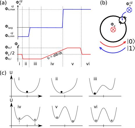
Figure 1: Schematics of (a) the pulse sequence for the LZ measurements, (b) a CJJ RF-SQUID qubit, and (c) the qubit potential during the measurement.

We have experimentally tested the above predictions by examining LZ transitions using a single qubit in a 28 qubit chip designed for adiabatic quantum computation. The sample was cooled down in a magnetically shielded dilution refrigerator with heavily filtered lines to a base temperature of about 10 mK. The qubits on the chip were compound Josephson junction (CJJ) RF-SQUID qubits as schematically shown in Fig. 1b and described in Ref. Harris07, . Each qubit consists of a main loop and CJJ loop subjected to external flux biases $\Phi_{x}$ and $\Phi_{x}^{\text{cjj}}$, respectively. The CJJ loop is interrupted by two nominally identical Josephson junctions connected in parallel. This device can be operated as a qubit for $\Phi_{x}^{\text{cjj}}\in[0.5,1]\Phi_{0}$ and $\Phi_{x}\approx 0$, where $\Phi_{0}$ is the flux quantum. The two oppositely circulating persistent current states correspond to the states $\left|0\right>$ and $\left|1\right>$. The bias energy is $\epsilon=2\left|I_{p}\right|\Phi_{x}$, where the $I_{p}$ is the magnitude of the persistent current. The parameter $\Delta$ is the amplitude of the flux tunneling between the two states. Both $\left|I_{p}\right|$ and $\Delta$ are controlled by $\Phi_{x}^{\text{cjj}}$. Maximum $\Delta\sim\omega_{p}\sim 20$ GHz, where $\omega_{p}$ is the plasma frequency of the RF-SQUID, is obtained at $\Phi_{x}^{\text{cjj}}=\Phi_{0}/2$. For $\Phi_{x}^{\text{cjj}}\approx\Phi_{0}$ one expects $\Delta\rightarrow 0$ and the system becomes localized in $\left|0\right>$ or $\left|1\right>$. One can then read out the qubit by measuring the flux via an inductively coupled DC-SQUID (not shown).

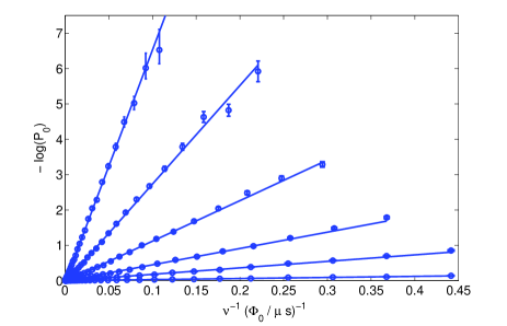
Figure 2: LZ probability as a function of inverse sweep rate for different values of $\Delta$ ($\Phi_{x}^{cjj}$ from $-0.925\Phi_{0}$ to $-0.91\Phi_{0}$). The lines are linear fits to the data.

We isolated one of the qubits by tuning the coupling between that qubit and its neighboring qubits to zero, which allowed us to perform single qubit LZ measurement using the pulse sequence shown in Fig. 1a. The qubit is first initialized in one of the states $|0\rangle$ or $|1\rangle$ at a bias $\Phi_{x}=\Phi_{x,i}$ where the transition out of the state is very unlikely, and then the bias is linearly swept from $\Phi_{x,i}$ to a final value $\Phi_{x,f}$, at which point the qubit is measured. A cartoon of the qubit potential during the pulse sequence is shown in Fig. 1c. The probability $P_{0}(t_{f})$ of finding the qubit in the same state $|0\rangle$ as it started from was measured by repeating the above process 2048 times for each value of the sweep rate $\nu$. Figure 2 shows the probability $P_{0}(t_{f})$ in logarithmic scale as a function of $1/\nu$. The result shows exponential dependence upon $1/\nu$, in agreement with Eq. (8).

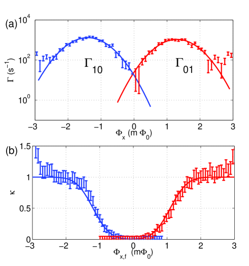
Figure 3: (a) First MRT peaks in $\Gamma_{01}$ and $\Gamma_{10}$ and their best fit with Eq. (4). (b) The experimental value of $\kappa$ as defined in (8) as a function of the final bias $\epsilon_{f}$. The solid line shows the theoretical curve (10) using the parameters obtained from the best fit in (a).

Next we experimentally verify equation (10). We first determine $\Delta$, $W$ and $\epsilon_{p}$ by measuring $\Gamma_{01}$ and $\Gamma_{10}$, as described in Ref. Harris07, . Figure 3a shows example plots of $\Gamma_{01}$ and $\Gamma_{10}$ as a function of bias $\Phi_{x}$ for the above qubit at $\Phi_{x}^{\text{cjj}}=-0.749\ \Phi_{0}$. The line-shape of the resonant peak fits very well with the Gaussian function (4), providing $\Delta,W$, and $\epsilon_{p}$ as fitting parameters. For the data shown in Fig. 3a, we found $\Delta=0.082\pm 0.002$ mK, $W=123\pm 2$ mK, and $\epsilon_{p}=354\pm 3$ mK. Equation (6) then gives the effective temperature of the sample to be $T=21\pm 1$ mK. Notice that the condition $T\ll W\ll 2\epsilon_{p}$ is approximately satisfied and therefore (8) should be sufficient to describe the LZ probability.

The LZ probability as a function of flux bias was then measured for the same CJJ setting as in Fig. 3a. Figure 3b shows $\kappa=-\ln P_{0}/(\pi\Delta/2\nu)$ as a function of $\Phi_{x,f}$ using the extracted $\Delta$. The data starts from zero where $\Phi_{x,f}\approx\Phi_{x,i}$ and shows a plateau at $\kappa\approx 1$, in agreement with the theory. We have also plotted, on the same graph, the theoretical prediction of Eq. (10), using $\epsilon_{p}$ and $W$ extracted from the MRT in Fig. 2a, and found very good agreement with the experiment with no extra fitting parameters. At larger biases, $|\Phi_{x,f}|>2.5\ \mathrm{m}\Phi_{0}$, the experimental $\kappa$ deviates from the theoretical curve due to tunneling to the first excited state in the target well.

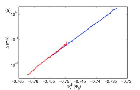
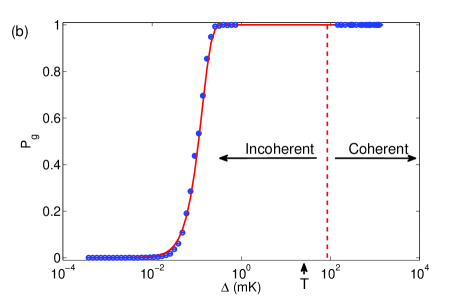
Figure 4: (a) Plot of $\Delta$ vs. flux bias $\Phi_{x}^{cjj}$ applied to the compound junction. The lower curve is $\Delta$ measured with MRT and the upper curve is $\Delta$ measured with LZ. (b) Experimental (dots) and theoretical (line) ground state probability $P_{g}=1-P_{\rm LZ}$, for fixed $\nu=0.05\Phi_{0}/\mu s$ as a function of $\Delta$. The dashed line indicates the crossover between the incoherent and coherent regime, defined by $W\approx\Delta$.

The measurements of the transition rates and the LZ probability allow us to extract $\Delta$ as a function $\Phi_{x}^{\text{cjj}}$ for a large range of $\Delta$ . Exponential dependence on $\Phi_{x}^{\text{cjj}}$ is evident in Fig. 4a. Figure 4b plots the LZ probability, for a fixed value of $\nu$, as a function of $\Delta$ for a quite wide range of $\Delta$ (from 27 $\mu$K to 1.25 K) together with the theoretical prediction . In the figure we have identified a line $\Delta=W$ which separates coherent tunneling from incoherent tunneling regime. Excellent agreement with theory is observed.

We have reported on an experimental probe of the practically interesting regime for adiabatic quantum computation, where the energy gap $\Delta$ is much smaller than both the decoherence induced energy level broadening $W$ and temperature $T$. The method used isolates a single qubit in a larger-scale adiabatic quantum computer, tunes its tunneling amplitude $\Delta$ into the $\Delta\ll W,T$ limit, and forces it to undergo a LZ transition. We find that the transition probability for the qubit quantitatively agrees with the theoretical predictions. In particular, we demonstrate that in this large decoherence limit, the quantum mechanical behavior of this qubit is the same (except for possible renormalization of $\Delta$) as that of a noise-free qubit, as long as the energy bias sweep covers the entire region of broadening $W$. The close agreement between theory and experiment for a single qubit undergoing a LZ transition in the presence of noise supports the accuracy of our dynamical models, including both the noise model and the model of a single superconducting qubit that has been isolated from its surrounding qubits in an adiabatic quantum computer. Future experiments will test the behavior of multiple coupled qubits undergoing a LZ transition in the presence of noise.

The authors are grateful to D.V. Averin for fruitful discussions. Samples were fabricated by the Microelectronics Laboratory of the Jet Propulsion Laboratory, operated by the California Institute of Technology under a contract with NASA.

References

- (1) E. Farhi, J. Goldstone, S. Gutmann, J. Lapan, A. Lundgren, and D. Preda, Science 292, 472 (2001).
- (2) D. Aharonov, W. van Dam, J. Kempe, Z. Landau, and S. Lloyd, SIAM J. Comput. 37, 166 (2007).
- (3) L.D. Landau, Phys. Z. Sowjetunion 2, 46 (1932).
- (4) C. Zener, Proc. R. Soc. A 137, 696 (1932).
- (5) M. Neilson and I. Chuang, Quantum Computation and Quantum Information, Cambridge University Press (2000).
- (6) A.M. Childs, E. Farhi, and J. Preskill, Phys. Rev. A 65, 012322 (2001).
- (7) M.H.S. Amin, P.J. Love, and C.J.S. Truncik, Phys. Rev. Lett. 100, 060503 (2008).
- (8) M.H.S. Amin and D.V. Averin, arXiv:0708.0384.
- (9) M.H.S. Amin, C.J.S. Truncik, and D.V. Averin, arXiv:0803.1196.
- (10) A. Izmalkov, M. Grajcar, E. Il’ichev, N. Oukhanski, Th. Wagner, H.-G. Meyer, W. Krech, M.H.S. Amin, A. Maassen van den Brink, A.M. Zagoskin, Europhys. Lett. 65, 844 (2004).
- (11) W.D. Oliver, Y. Yu, J.C. Lee, K.K. Berggren, L.S. Levitov, T.P. Orlando, Science 310, 1653 (2005).
- (12) M. Sillanpää, T. Lehtinen, A. Paila, Yu. Makhlin, and P. Hakonen, Phys. Rev. Lett. 96, 187002 (2006).
- (13) A.J. Leggett et al., Rev. Mod. Phys. 59, 1 (1987).
- (14) U. Weiss, “Quantum Dissipative Systems”, World Scientific, Singapore, 2nd edition (1999).
- (15) P. Ao and J. Rammer, Phys. Rev. B 43, 5397 (1991).
- (16) M.H.S. Amin and D.V. Averin, Phys. Rev. Lett. 100, 197001 (2008).
- (17) R. Harris, M.W. Johnson, S. Han, A.J. Berkley, J. Johansson, P. Bunyk, E. Ladizinsky, S. Govorkov, M.C. Thom, S. Uchaikin, B. Bumble, A. Fung, A. Kaul, A. Kleinsasser, M.H.S. Amin, and D.V. Averin, arXiv:0712.0838.