Heisenberg antiferromagnets with uniaxial exchange and cubic anisotropies in a field

Abstract

Classical Heisenberg antiferromagnets with uniaxial exchange anisotropy and a cubic anisotropy term in a field on simple cubic lattices are studied with the help of ground state considerations and extensive Monte Carlo simulations. Especially, we analyze the role of non–collinear structures of biconical type occurring in addition to the well–known antiferromagnetic and spin–flop structures. Pertinent phase diagrams are determined, and compared to previous findings.

1 Introduction

Uniaxially anisotropic Heisenberg antiferromagnets in a magnetic field have been studied quite extensively in the past, both experimentally and theoretically. Typically, they display, at low temperatures, the antiferromagnetic phase and, when increasing the field, the spin–flop phase [1]. A prototypical model describing these phases is the Heisenberg model with a uniaxial exchange anisotropy, the XXZ model

$${\cal H}_{\mathrm{XXZ}}=J\sum\limits_{i,j}\left[\,\Delta(S_{i}^{x}S_{j}^{x}+S_{i}^{y}S_{j}^{y})+S_{i}^{z}S_{j}^{z}\,\right]\;-\;H\sum\limits_{i}S_{i}^{z}$$ (1)

where $J$ is the exchange coupling between classical spins, $(S_{i(j)}^{x},S_{i(j)}^{y},S_{i(j)}^{z})$, of length one at neighboring sites, $i$ and $j$, of a simple cubic lattice, $\Delta$ is the exchange anisotropy, $1>\Delta>0$, and $H$ is the applied magnetic field along the easy axis, the $z$–axis.

Figure 1: Spin orientations on neighboring sites showing antiferromagnetic (a), biconical (b), and spin–flop (c) ground state structures of the XXZ model.

The phase diagram of the model has been studied several years ago, using mean–field theory [2], Monte Carlo simulations [3], and high temperature series expansions [4], suggesting the transition between the antiferromagnetic (AF) and spin–flop (SF) phases to be of first order and the boundaries of the paramagnetic phase to the AF and SF phases to be continuous transitions in the Ising and XY universality classes. Based on renormalization group analysis in one loop order, a bicritical point in the Heisenberg universality class has been proposed, at which the three different phases meet [5, 6]. However, this scenario has been scrutinized when doing renormalization group calculations in high loop order [7], where the bicritical point is found to be unstable against a ’tetracritical biconical point’ [6], which, in turn, may be unstable towards transitions of first order in the vicinity of the multicritical point of the three phases. The seemingly conflicting descriptions may be reconciled by a new renormalization group analysis in two loop order [8].

As has been noted very recently [9, 10, 11], not only AF and SF phases, but also ’biconical’ (BC) structures, see Fig. 1, may play an important role in the XXZ model. Indeed, such BC structures are degenerate ground states at the critical field separating AF and SF configurations at zero temperature. For the XXZ model on a square lattice, these degenerate BC fluctuations seem to lead to a narrow disordered phase intervening between the AF and SF phases at low temperatures [9, 12, 13]. The importance of BC structures for the three–dimensional XXZ antiferromagnet, where they are also present as degenerate ground states at the special field, had not been studied in any detail so far.

Biconical structures may be ground states even in a finite range of magnetic fields, giving then rise to an ordered BC phase at low temperatures, when introducing in the XXZ model further anisotropy terms or longer–range exchange interactions, as it is known for many years [14, 15]. This feature has been confirmed in recent simulations when adding a quadratic single–ion anisotropy to the XXZ model on the square lattice [10, 11]. The related lowest–order single–ion term of cubic symmetry may be written in the form [16, 17]

$${\cal H}_{\mathrm{CA}}=F\sum\limits_{i}\left[(S_{i}^{x})^{4}+(S_{i}^{y})^{4}+(S_{i}^{z})^{4}\right]$$ (2)

where $F$ denotes the strength of the ’cubic anisotropy’. The sign of $F$ determines whether the spins tend to align along the cubic axes, for $F<0$, or, for $F>0$, in the diagonal directions of the lattice. Because of these tendencies, the BC structures show no full rotational invariance in the $xy$–plane perpendicular to the easy axis, the $z$–axis, in contrast to the XXZ case.

When an ordered BC phase exists at low temperatures, for example due to the cubic anisotropy, intricate multicritical behavior may show up, including a tetracritical biconical point, at which the AF, SF, BC, and paramagnetic phases meet, as has been discussed before [15, 18, 19, 20], applying mean-field theory and renormalization group arguments.

Experimentally, many antiferromagnets with uniaxial anisotropy have been investigated, quasi two–dimensional magnets [21, 22, 23] as well as three–dimensional magnets such as GdAlO₃, NiCl₂4H₂O, MnF₂ or Mn₂(Si,Ge)S₄ [24, 25, 26, 27, 28]. While we shall deal here with the theoretical analysis of the models, results may turn out to be useful for interpreting specific experiments in future work.

The aim of our paper is to study, especially, the role of biconical, non–collinear structures in three–dimensional classical Heisenberg antiferromagnets with uniaxial exchange anisotropy and cubic anisotropy. Both ground state considerations and Monte Carlo techniques are applied.

Figure 2: Ground states in the $(F,H)$–plane for the full Hamiltonian, ${\cal H}_{\mathrm{f}}$= ${\cal H}_{\mathrm{XXZ}}$ + ${\cal H}_{\mathrm{CA}}$, with exchange anisotropy $\Delta$= 0.8. The full circle denotes the highly degenerate point in the XXZ model.

The paper is organized as follows: First, results of ground state calculations are presented, and then Monte Carlo findings on thermal properties and phase diagrams will be discussed, for the XXZ model and its extension. The article will be concluded by a short summary.

2 Ground state properties

The ground states of the full Hamiltonian, ${\cal H}_{\mathrm{f}}$= ${\cal H}_{\mathrm{XXZ}}$ + ${\cal H}_{\mathrm{CA}}$, eqs. (1) and (2), may be determined by minimization of the energy, e.g., with respect to the azimuthal angle, $\phi$, i.e. the angle between the projection of the spin vector in the $xy$–plane and the $x$–axis, and the $z$–component of the spin vector [14, 29]. As usual, we consider spin structures with two sublattices, $A$ and $B$, where neighboring sites on the cubic lattice belong to different sublattices. In general, the minimization may be easily done numerically.

In Fig. 2, resulting ground states in the $(F,H)$–plane are depicted, setting the exchange anisotropy $\Delta$ equal to 0.8, as before [3, 9, 12].

Figure 3: Sketch of discretized biconical structures for antiferromagnets with cubic anisotropy, ${\cal H}_{\mathrm{f}}$, in the case of (a) $F>0$, BC2, and (b) $F<0$, BC1.

In the case of a vanishing cubic anisotropy, $F=0$, i.e. for the XXZ antiferromagnet, one encounters, when increasing the field, AF, SF, and ferromagnetic ground state configurations. In complete analogy to the model on a square lattice, the ground state is highly degenerate in BC structures at the critical field $H_{c}$ separating the AF and SF structures, see Figs. 1 and 2. For cubic lattices, one has $H_{c}=6J\sqrt{1-\Delta^{2}}$. The non–collinear BC spin structures may be characterized by two different polar or tilt angles of the spin vectors on the two sublattices $A$ and $B$, $\Theta_{A}$ and $\Theta_{B}$, as shown in Fig. 1(b). Obviously, for the SF structures, the angles are identical, $\Theta_{A}=\Theta_{B}=\Theta_{SF}$, depicted in Fig. 1(c). At $H_{c}$, the two tilt angles of the degenerate BC structures are interrelated by

$$\Theta_{B}=\arccos\left(\frac{\sqrt{1-\Delta^{2}}\;-\;\cos\Theta_{A}}{1\;-\;\sqrt{1-\Delta^{2}}\cos\Theta_{A}}\right)$$ (3)

interpolating continuously between the AF and SF configurations, when varying one of the tilt angles [9, 10]. Of course, the rotational invariance of the spin components in the $xy$–plane leads to an additional degeneracy in the BC and SF configurations.

Let us now consider positive values of $F$, $F>0$. For vanishing field, $H$= 0, and $F/J>0.3$, see Fig. 2, the simple AF structure is replaced by a tilted antiferromagnetic (TAF) configuration. Spins on the two sublattices point still in opposite directions, but not along the easy axis. Indeed, the spins are oriented more and more towards diagonals of the lattice with increasing positive cubic anisotropy $F$ [29]. Applying, for $F>0$, an external field, BC structures may occur, in which neighboring spins have different tilt angles, $\Theta_{A}$ and $\Theta_{B}$. In contrast to the XXZ case, there is no full rotational symmetry in the azimuthal angles, $\phi$, of the spins. Instead, for $F>0$, the spins order along the diagonals of the lattice, and $\phi$ is discretized, taking the values, $(2n+1)\pi/4$, where $n$ is an integer. The $xy$–spin components are ordered antiferromagnetically, $\phi_{B}$= $\phi_{A}+\pi$. The resulting discretized biconical structure, BC2, is sketched in Fig. 3(a). Obviously, the SF configurations are discretized in the azimuthal angle in the same way as the BC structures. When fixing $F$ and varying the field $H$, the two tilt angles, $\Theta_{A}$ and $\Theta_{B}$, change continuosly when going from the AF (or TAF) to the BC2 structures. In the BC2 region, the tilt angles, $\Theta_{A}$ and $\Theta_{B}$, vary continuously as well. On the other hand, they seem to jump when going from the BC2 to the SF region. Note that the tilt angle of the SF structure, $\Theta_{SF}$, at the border to the BC2 region, see Fig. 2, depends only weakly on the strength $F$ of the cubic anisotropy.

For $F<0$, the azimuthal angles of the spins, both for biconical and SF structures, take the values $\phi=n\pi/2$, $n$ being an integer, reflecting the fact that the cubic anisotropy now favors alignment of the spins along the cubic axes. The $xy$–spin components are ordered antiferromagnetically, $\phi_{B}$= $\phi_{A}+\pi$, as for $F>0$. Biconical ground states occur for sufficiently strong negative values of $F$, as shown in Fig. 2. The resulting BC1 structure is shown in Fig. 3(b). The tilt angles $\Theta_{A}$ and $\Theta_{B}$ change continuously in the BC1 region, when varying the cubic anisotropy $F$ and the field $H$. At the boundaries of the BC1 region to the SF, AF, and ferromagnetic regions the tilt angles seem to jump, except between the BC1 and SF regions near the triple point of these two and the ferromagnetic regions, see Fig. 2.

3 Monte Carlo simulations

Figure 4: Phase diagram of the XXZ model on a cubic lattice with exchange anisotropy $\Delta=0.8$, as obtained from Monte Carlo simulations described in the text.

In our simulations of thermal properties of the XXZ and the full model, ${\cal H}_{\mathrm{f}}$, we applied the Metropolis algorithm with single–spin–flips. Lattices of $L^{3}$ sites, employing periodic boundary conditions, with $L$ ranging from 4 to 32, allowed to do useful finite–size analyses. To obtain thermal averages, we performed, at fixed model parameters and temperature, several independent runs, with distinct random numbers, each run consisting of, at least, $10^{7}$ Monte Carlo steps per site for the larger systems.

We recorded standard thermodynamic quantities such as the specific heat, $C$, the (absolute) total magnetization, $m$, longitudinal, $m^{z}_{st}$, and transverse, $m^{xy}_{st}$, staggered magnetizations, being the order parameters in the AF and SF phases, as well as the corresponding susceptibilities, $\chi$, $\chi^{z}_{st}$, and $\chi^{xy}_{st}$. In addition, we computed the Binder cumulants [30] of the two different order parameters, $U_{z}$ and $U_{xy}$, and related histograms. To gain microscopic insights, especially, on BC structures, we also recorded probability functions of the tilt angles, such as the probability $p_{2}(\Theta_{A},\Theta_{B})$ for finding the two angles, $\Theta_{A}$ and $\Theta_{B}$, at neighboring sites, and the probability $p(\Theta)$ for encountering the tilt angle $\Theta$ [9, 10, 11].

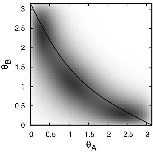
Figure 5: Grayscale representation of the probability $p_{2}$ for finding the tilt angles $\Theta_{A}$ and $\Theta_{B}$ at neighboring sites in the XXZ model with $\Delta=0.8$ in the vicinity of the transition between the AF and SF phases, at $k_{B}T/J=0.7$ and $H/J=3.6925$. The solid line corresponds to eq. (3). The system size is $L=24$.

Let us first consider the XXZ model on a cubic lattice, eq. (1). Its phase diagram has been determined, using Monte Carlo techniques, already some time ago [3]. Certainly, in present simulations the accuracy has been improved significantly. The resulting phase diagram is depicted in Fig.4, where the phase boundaries have been estimated by standard finite–size extrapolations [31] for thermodynamic quantities and the Binder cumulant. The phase boundary lines deviate somewhat from the ones estimated before [3], which we attribute to the improved statistics of the present study.

We also identified the type of transitions and, in the case of continuous transitions, their universality classes, by monitoring, e.g., the finite size–dependences of the peak heights of the susceptibilities and specific heat, to estimate critical exponents, see below.

In agreement with previous suggestions [3, 13], the transition between the AF and SF phases is found to be of first order, with, for instance, the maximal staggered susceptibilities increasing with system size proportionally to $L^{3}$, characteristic for such transitions [32]. Moreover, as a remainder of the degeneracy of the ground state at $H_{c}$, biconical structures prevail near that transition at low temperatures, as one may easily observe in $p_{2}$, see Fig. 5. As included in the figure, the dominant BC fluctuations are quite close to those expected from the degenerate ground states, eq. (3). Note that $p_{2}$ displays simultaneously local maxima at positions belonging to the AF and SF structures, as shown in Fig. 5. The phenomenon gets more pronounced when increasing the system size, and it reflects coexistence of the AF and SF phases at a first–order transition. This behavior is in marked contrast to that of the XXZ antiferromagnet on a square lattice, where the BC fluctuations seem to lead to a disordered phase between the AF and SF phases [9, 10, 12, 13].

The transition from the paramagnetic phase to the AF phase is found to be in the Ising universality class, while the transition from the paramagnetic phase to the SF phase is found to belong to the XY universality class. For instance, we estimated canonical [31] asymptotic critical exponents describing the size dependence of the peak height of the staggered susceptibilties, $(\gamma/\nu)^{z}=d(\ln\chi^{z})/d(\ln L)$, $L\rightarrow\infty$, and analogously for the transverse susceptibility, see Fig. 6. Our estimates agree nicely with the known, accurate values obtained from renormalization group calculations in high loop order for both universality classes [33]. Similarily, our estimates [29] for the critical Binder cumulants $U^{*}_{z}$ and $U^{*}_{xy}$ at the two types of transitions are close to those obtained for the three–dimensional nearest–neighbor Ising and XY models [34, 35]. Note, that the critical Binder cumulant may change, within a given universality class, due to, e.g., spatially anisotropic interactions [36, 37]. This possible pitfall seems to play no role in the XXZ model.

Figure 6: Effective critical exponent $(\gamma/\nu)^{z}_{eff}(L)=d\ln\chi^{z}/d\ln L$ of the staggered longitudinal susceptibility, to locate the multicritical point in the XXZ model. The arrow marks the asymptotic critical exponent in the Ising universality class [33].

Analyzing critical exponents and critical Binder cumulants, we locate the multicritical point at $k_{B}T/J=1.025\pm 0.015$ and $H/J=3.90\pm 0.03$, improving the previous estimate [3]. To obtain the estimate, we proceed as exemplified for $\chi^{z}_{st}$ in Fig. 6. We determine the effective, size–dependent critical exponent $(\gamma/\nu)^{z}_{eff}(L)=d(\ln\chi^{z})/d(\ln L)$ of the height of the peak in the staggered longitudinal susceptibility $\chi^{z}_{st}$ for the simulated system sizes at various fixed temperatures close to the boundary of the AF phase. One observes a pronounced increase of the effective exponent in a small interval of temperatures. This behavior signals the change from a continuous transition of Ising type, with $(\gamma/\nu)^{z}\approx 1.9635$ [33], to a transition of first order, where the asymptotic exponent is expected to be 3. A pronounced increase occurs simultaneously, within the temperature resolution of the simulations, for the effective exponent of the staggered transverse susceptibility [29]. Accordingly, it indicates a transition of first order between the AF and SF phases. The ratio of the two staggered susceptibilities exhibits an extremum which height is largely independent of system size in the vicinity of the multicritical point. Such a behavior seems to be consistent with a bicritical Heisenberg point.

These observations and interpretations on the character of the multicritical point have to be viewed with care, having in mind controversial renormalization group arguments. Early renormalization group calculations in one loop order suggested a bicritical Heisenberg point [5, 6]. Later work, in five loop order, found the biconical point to be the stable one [7, 38], however, not ruling out a triple point, at which at least one of the transition lines to the paramagnetic phase is, eventually close to the multicritical point, of first order. A most recent analysis indicates that all three scenarios are possible, depending on the model parameters [8]. In our case, $\Delta=0.8$, the Monte Carlo simulations seem to favor a bicritical point, with Ising and XY lines of the paramagnetic phase meeting the line of first order between the AF and SF phases. Of course, a crossover to a different multicritical behavior in the immediate vicinity of the multicritical point may happen. Simulational clarification of this aspect may need an enormous amount of computer time.

Figure 7: Phase diagram of the XXZ model, $\Delta=0.8$, with a positive cubic anisotropy $F$ at fixed field, $H/J$ =1.8.

Let us now turn to the Monte Carlo results for the full Hamiltonian, ${\cal H}_{\mathrm{f}}$= ${\cal H}_{\mathrm{XXZ}}$ + ${\cal H}_{\mathrm{CA}}$, eqs. (1) and (2), including exchange and cubic anisotropies. We simulated thermal properties for a few selected cases, where discretized biconical structures play an important role. As before, we set the exchange anisotropy $\Delta$ equal to 0.8.

For positive cubic anisotropy, $F>0$, favoring orientations of the spins along the diagonals of the cubic lattice, a discretized ordered BC2 phase may arise from the corresponding ground state, see Fig. 2. This behavior is illustrated in Fig. 7, when fixing the field, $H/J$= 1.8, and varying $F$. At small values of $F$, there is an AF ordering at low temperatures. Above a critical value of $F$, $F>F_{c}(H=1.8J)=0.218..J$, the low–temperature phase is, indeed, of BC2 type. In that case, increasing the temperature at fixed $F$, one goes from the BC2 to the AF phase before then entering the disordered paramagnetic phase. The transitions between the two ordered phases and between the AF and disordered phases have been located from monitoring the staggered magnetizations and susceptibilities, the specific heat, and Binder cumulants. An example is shown in Fig.8, where the staggered longitudinal and transverse magnetizations are displayed, as a function of temperature, at $F/J$= 1.0. At the transition between the AF and BC2 phases, the absolute staggered transverse magnetization, $|m^{xy}_{st}|$, drops rather sharply, with an accompanying anomaly in the absolute staggered longitudinal magnetization, $|m^{z}_{st}|$. The staggered longitudinal magnetization is the order parameter of the AF phase, and it decreases rapidly on approach to the paramagnetic phase.

Figure 8: Absolute staggered longitudinal and transverse magnetizations as a function of temperature at fixed field, $H/J$= 1.8, and at fixed cubic anisotropy $F/J$= 1.0. Systems with $16^{3}$ sites have been simulated. Note that error bars are small compared to symbol sizes.

As expected, the transition from the AF to the disordered phase seems to be Ising like, as follows, e.g. from the critical exponent describing the size–dependence of the height of the peak in $\chi^{z}_{st}$. The transition from the BC2 to the AF phase is found to be consistent with the XY universality class [29]. Indeed, the transition between the AF and biconical phases has been predicted to belong to the XY universality class in an early renormalization group analysis [19]. Furthermore, the cubic anisotropy is expected [33, 39] to be an irrelevant perturbation in the three–dimensional XY case. As depicted in Fig.7, there is no multicritical point of the three phases at the values of $F$ we studied.

A multicritical point may occur in the $(H,T)$–plane, when fixing $F$, $F>0$. Indeed, our simulation results, especially at $F/J=0.15$ and 1.5 [29], show a phase diagram comprising the AF, BC2, SF, and paramagnetic phases. However, much more extensive simulations, being beyond the scope of the present study, would be needed to study the possible multicritical points in detail. Especially, the order of the transition between the BC2 and SF phases deserves a careful analysis. A transition of first order, as suggested by the ground state analysis, would preclude a tetracritical point [19].

Finally, we briefly mention results for the case of negative cubic anisotropy, $F<0$, favoring spin orientations along the cubic axes. As follows from the ground state considerations, see Fig.2, biconical structures only show up at relatively large negative values of $F$. Moreover, the tilt angles usually seem to jump when going from the BC1 region to one of its neighboring, i.e., ferromagnetic, AF, or SF, regions.

Our Monte Carlo simulations, especially at $F/J$= -2 and varying the field at fixed temperatures [29], suggest that there is an ordered BC1 phase which, however, gets destabilized at quite low temperatures. Thorough analyses of full phase diagrams and the types of the transition are well beyond the scope of the present work.

4 Summary

Classical Heisenberg antiferromagnets on cubic lattices with uniaxial exchange, $\Delta$, and cubic, $F$, anisotropies in a magnetic field, $H$, have been studied, using ground state considerations and Monte Carlo techniques.

In addition to antiferromagnetic (AF) and spin–flop (SF) structures non–collinear, biconical (BC) structures are observed, depending on the strength of the anisotropies, the field, and temperature. They may occur as ground states, which, at low temperatures, may contribute to thermal fluctuations of BC type or may give rise to ordered BC phases.

Specifically, in the XXZ antiferromagnet ($F$= 0) biconical structures are present as degenerate ground states at the critical field separating the AF and SF states. At low temperatures near the transition between the AF and SF phases, BC fluctuations show up, but they do not lead to a distinct phase, in contrast, for instance, to the situation for the XXZ magnet on a square lattice, where the AF and SF phases are separated by a narrow disordered phase. Moreover, in this study, the multicritical point of the three–dimensional XXZ model, at which the AF, SF, and paramagnetic phases meet, has been located accurately for $\Delta$= 0.8. That point seems to have bicritical character, being the intersection of two continuous transition lines between the AF and SF phases to the paramagnetic phase with a transition line of first–order between the AF and SF phases. Note that we did not rule out a crossover to a different character in the immediate vicinity of the multicritical point.

The cubic anisotropy $F$ may lead, depending on its sign, to a tendency of the spin orientations along the diagonals of the lattice, $F>0$, or along the cubic axes, $F<0$. In both cases, BC as well as SF structures have now discretized preferred orientations of the $xy$–components of the spins, thereby breaking the rotational symmetry of the XXZ model.

For positive cubic anisotropy, $F>0$, biconical configurations occur as ground states next to the SF and AF phases, giving rise to an ordered BC2 phase. The transition to the AF phase is found to be consistent with being in the XY universality class, where the cubic anisotropy is expected to be an irrelevant perturbation. Phase diagrams with three ordered phases, AF, SF, and BC2, and a paramagnetic phase have been determined.

At small negative cubic anisotropy, $F<0$, there are no biconical ground states. However, such structures, of BC1 type, may be stabilized at larger negative values of $F$, between the ferromagnetic and the AF or SF ground states. The biconical ground states then give rise to an ordered BC1 phase at sufficiently low temperatures.

Acknowledgements

We should like to thank Martin Holtschneider, David Landau, and David Peters for useful discussions. We also thank Reinhard Folk for very helpful conversations and information on pertinent calculations prior to publication.

References

- [1] L. Néel, Ann. Phys.-Paris 5, 232 (1936).
- [2] C. J. Gorter and T. van Peski-Tinbergen, Physica (Utr.) 22, 273 (1956).
- [3] D. P. Landau and K. Binder, Phys. Rev. B 17, 2328 (1978).
- [4] O. G. Mouritsen, E. K. Hansen, and S. J. K. Jensen, Phys. Rev. B 22, 3256 (1980).
- [5] M. E. Fisher and D. R. Nelson, Phys. Rev. Lett. 32, 1350 (1974).
- [6] J. M. Kosterlitz, D. R. Nelson, and M. E. Fisher, Phys. Rev. B 13, 412 (1976).
- [7] P. Calabrese, A. Pelissetto, and E. Vicari, Phys. Rev. B 67, 054505 (2003).
- [8] R. Folk, Yu. Holovatch, and G. Moser, Preprint (2008).
- [9] M. Holtschneider, S. Wessel, and W. Selke, Phys. Rev. B 75, 224417 (2007).
- [10] M. Holtschneider and W. Selke, Phys. Rev. B 76 (R), 220405 (2007).
- [11] M. Holtschneider and W. Selke, Eur. Phys. J. B 62, 147 (2008).
- [12] C. Zhou, D. P. Landau, and T. C. Schulthess, Phys. Rev. B 74, 064407 (2006).
- [13] M. Holtschneider, W. Selke, and R. Leidl, Phys. Rev. B 72, 064443 (2005).
- [14] H. Matsuda and T. Tsuneto, Prog. Theor. Phys. Supplement 46, 411 (1970).
- [15] K.-S. Liu and M. E. Fisher, J. Low. Temp. Phys. 10, 655 (1973).
- [16] F. Keffer, in Handbuch der Physik, ed. by S. Flügge (Springer, Berlin, 1966), Vol. XVIII, Pt.2, p.1.
- [17] A. Aharony, Phys. Rev. B 8, 4270 (1973).
- [18] F. Wegner, Solid State Commun. 12, 785 (1973).
- [19] A. D. Bruce and A. Aharony, Phys. Rev. B 11, 478 (1975).
- [20] A. Aharony, J. Stat. Phys. 110, 659 (2003).
- [21] L. J. de Jongh (ed.), Magnetic properties of layered transition metal compounds, (Klüwer, Dordrecht, 1990).
- [22] T. Thio, C. Y. Chen, B. S. Freer, D. R. Gabbe, H. P. Jenssen, M. A. Kastner, P. J. Picone, N. W. Preyer, and R. J. Birgeneau, Phys. Rev. B 41, 231 (1990).
- [23] T. Kroll, R. Klingeler, J. Geck, B. Büchner, W. Selke, M. Hücker, and A. Gukasov, J. Magn. Magn. Mat. 290, 306 (2005).
- [24] H. Rohrer and C. Gerber, Phys. Rev. Lett. 38, 909 (1977).
- [25] C. C. Becerra, N. F. Oliveira, A. Paduan-Filho, W. Figueiredo, and M. V. Souza, Phys. Rev. B 38, 6887 (1988).
- [26] G. P. Felcher and R. Kleb, Europhys. Lett. 36, 455 (1996).
- [27] K. Ohgushi and Y. Ueda, Phys. Rev. Lett. 95, 217202 (2005).
- [28] Z. W. Ouyang, V. K. Pecharsky, K. A. Gschneidner, D. L. Schlagel, and T. A. Lograsso, Phys. Rev. B 76, 134415 (2007).
- [29] G. Bannasch, Diploma thesis, RWTH Aachen (2008).
- [30] K. Binder, Z. Physik B 43, 119 (1981).
- [31] M. N. Barber, in Phase Transitions and Critical Phenomena, ed. by C. Domb and J. L. Lebowitz (Academic Press, New York, 1983), Vol. 8.
- [32] K. Vollmayr, J. D. Reger, M. Scheucher, and K. Binder, Z. Physik B 91, 113 (1993).
- [33] A. Pelissetto and E. Vicari, Phys. Rep. 368, 549 (2002).
- [34] M. Hasenbusch, K. Pinn, and S. Vinti, Phys. Rev. B 59, 11471 (1999).
- [35] M. Hasenbusch and T. Török, J. Phys. A 32, 6361 (1999).
- [36] X. S. Chen and V. Dohm, Phys. Rev. E 70, 056136 (2004); V. Dohm, Phys. Rev. E 77, 061128 (2008).
- [37] W. Selke and L. N. Shchur, J. Phys. A: Math. Gen.38, L739 (2005).
- [38] A. Pelissetto and E. Vicari, Phys. Rev. 76, 024436 (2007).
- [39] J. M. Carmona, A. Pelissetto, and E. Vicari, Phys. Rev. B 61, 15136 (2000).