Adaptive multiresolution schemes with local time stepping for two-dimensional degenerate reaction-diffusion systems

Abstract.

We present a fully adaptive multiresolution scheme for spatially two-dimensional, possibly degenerate reaction-diffusion systems, focusing on combustion models and models of pattern formation and chemotaxis in mathematical biology. Solutions of these equations in these applications exhibit steep gradients, and in the degenerate case, sharp fronts and discontinuities. This calls for a concentration of computational effort in zones of strong variation.

The multiresolution scheme is based on finite volume discretizations with explicit time stepping. The multiresolution representation of the solution is stored in a graded tree (“quadtree”), whose leaves are the non-uniform finite volumes on the borders of which the numerical divergence is evaluated. By a thresholding procedure, namely the elimination of leaves that are smaller than a threshold value, substantial data compression and CPU time reduction is attained. The threshold value is chosen optimally, in the sense that the total error of the adaptive scheme is of the same slope as that of the reference finite volume scheme.

Since chemical reactions involve a large range of temporal scales, but are spatially well localized (especially in the combustion model), a locally varying adaptive time stepping strategy is applied. For scalar equations, this strategy has the advantage that consistence with a CFL condition is always enforced. Numerical experiments with five different scenarios, in part with local time stepping, illustrate the effectiveness of the adaptive multiresolution method. It turns out that local time stepping accelerates the adaptive multiresolution method by a factor of two, while the error remains controlled.

1. Introduction

Multiresolution techniques were first introduced by Harten [19] to improve the performance of schemes for one-dimensional conservation laws. Later on, these original ideas were extended to several kinds of related problems [2, 6, 10], leading finally to the concept of fully adaptive multiresolution schemes [13, 14, 30, 35]. Overviews on multiresolution methods for conservation laws are given by Chiavassa, Donat, and Müller [11] and Müller [30]. The basic aim of this approach is to accelerate a given finite volume scheme on a uniform grid at the cost of an at most controllable loss of accuracy, that is, the accelerated scheme should be of the same order than the original one. The principle of the multiresolution analysis is to represent a set of data given on a fine grid as values on a coarser grid plus a series of differences, called details, at different levels of nested dyadic grids. These differences contain information on the local regularity of the solution. An appealing feature of this data representation is that these details are small in regions where the solution is smooth. By thresholding small details (cells whose coefficients are smaller than a prescribed tolerance are removed), a locally refined adaptive grid is defined. This threshold is chosen such that the discretization error of the reference scheme is balanced with the accumulated thresholding error introduced in each time step. Significant speed-up of the computation and data compression is achieved for long-time evolution problems, large systems, multidimensional domains, and solutions with sharp fronts.

The present paper serves two purposes. On one hand, the adaptive multiresolution scheme for parabolic PDEs [35] and strongly degenerate parabolic PDEs in one space dimension [7, 8] is extended to two-dimensional systems of (possibly degenerate) parabolic PDEs. These equations produce solutions that vary smoothly wherever the solution causes the PDE to be parabolic, but produce sharp fronts, or even discontinuities, close to solution values at which the equation degenerates, so adaptive multiresolution methods are a proper device to efficiently capture these fronts. Similar features (that is, solutions with steep gradients) also appear in a combustion model of reaction-diffusion type. The analysis made in [37] is extended here to the study of two interacting flame balls. In this case, an adaptive strategy is equally very useful, especially when the flame front is well localized in space, since fine grids are only needed in small subregions of the computational domain. We will utilize then an adaptive multiresolution scheme applied to a reference finite volume discretization with explicit time integration.

On the other hand, chemical reactions are known to involve a large range of temporal scales, especially in long-time evolutions. Then an adaptive time stepping strategy is recommendable. Earlier efforts in this direction, which include [8, 12, 15, 18] and the references therein, were based on using the same time step to advance the solution on all parts of the computational domain, and controlling the time step through an embedded pair of Runge-Kutta schemes (known as Runge-Kutta-Fehlberg (RKF) schemes). In these procedures, one compares the numerical solution after each time step with an (approximate) reference solution, and adjusts the time step if the discrepancy is unacceptable. In contrast to this approach, we here adapt the locally varying time stepping strategy recently introduced for multiresolution schemes for conservation laws and multidimensional systems by Lamby, Müller, and Stiriba [24] and Müller and Stiriba [31]. This strategy is not precisely (time-)adaptive for scalar equations, since the time step for each level remains the same for all times. However, in the case of nonlinear systems, coupling of components entering the CFL condition makes it necessary to compute the time step after each iteration, according the evolving CFL condition, and therefore we have a scheme adaptive in time. Our results in terms of CPU time savings are encouraging and the strategy is consistent with a CFL condition, in contrast to the approach based one the RKF device. We mention that Müller and Stiriba [31] also combine local time stepping and multiresolution for implicit schemes, and that more details are also given in the germinal papers of Berger and Oliger [1], Osher and Sanders [34] and the references therein.

The remainder of this paper is organized as follows. In Section 2 the reaction-diffusion systems studied herein are briefly described. In Section 3 we present the reference finite volume methods to which we apply the multiresolution device, and in Section 4 the adaptive multiresolution strategy, as well as the required graded tree data structure, are outlined. In Section 5 we analyze the error of the adaptive multiresolution scheme, and deduce the optimal choice of the threshold. This choice ensures that the discretization error of the reference scheme is balanced with the accumulated thresholding error which is introduced in each time step. In Section 6 we address the local time stepping strategy applied to the multiresolution strategy, and in Section 7, we outline the overall multiresolution procedure. Finally, in Section 8 the method is applied to different scenarios. Example 1 corresponds to a single-species reaction diffusion equation, Examples 2 and 3 deal with the thermo-diffusive model for the interaction between flame balls, Examples 4 and 5 shows the results of Turing-type pattern formation produced by a reaction-diffusion system, and Example 6 arises from a model of chemotaxis with growth. Conclusions of our study are collected in Section 9. All numerical results clearly reveal high resolution and improvement in terms of compression of memory and savings in computational effort.

2. A class of reaction-diffusion systems

2.1. A single-species reaction-diffusion model

Model 1 is the following initial-boundary value problem for a scalar reaction-diffusion equation, where $\mathbf{x}=(x,y)$ and $(x,y,t)\in Q_{T}:=\Omega\times[0,T]$, $\Omega\subset\mathbb{R}^{2}$:

$$u_{t} =f(u,\mathbf{x})+\Delta A(u),$$ (2.1a)

$$u(\mathbf{x},0) =u_{0}(\mathbf{x})\quad\text{on $\Omega$},$$ (2.1b)

$$\nabla A(u)\cdot\mathbf{n} =0\quad\text{on $\Sigma_{T}:=\partial\Omega\times[0,T]$.}$$ (2.1c)

This problem may serve as a scalar prototype degenerate reaction-diffusion model. Here, the zero-flux boundary condition (2.1c) implies that the reaction-diffusion domain is isolated from the external environment. For $f(u,\mathbf{x})=f(u)$, (2.1a) appears in [33] in an ecological setting, where $u$ denotes the population density of a species, and $f(u)$ is its dynamics, where it is assumed that $f(0)=0$ and $f^{\prime}(0)\neq 0$. For example, $f(u)=u(1-u)-u^{2}/(1+u^{2})$ corresponds to the population dynamics of the spruce band-worm [33], and models the growth of the population by a logistic expression and the rate of mortality due to predation by other animals. We modify this expression by a radial spatial factor, and use

$$f(u,\mathbf{x}):=10\left(\exp(-5r)u(1-u)+\bigl{(}\exp(-5r)-1\bigr{)}\frac{u^{2}}{1+u^{2}}\right),\quad r:=\sqrt{(x-0.5)^{2}+(y-0.5)^{2}},$$ (2.2)

which means that the birth of individuals is concentrated near the center $(0.5,0.5)$, and mortality increases with increasing distance from the origin. On the other hand, most standard spatial models of population dynamics simply assume that $A(u)=Du$, where the constant diffusion coefficient $D>0$ measures the dispersal efficiency of the species under consideration. Motivated by Witelski [41], who advanced degenerate diffusion in the context of population dynamics, we utilize herein the strongly degenerate diffusion coefficient

$$A(u)=\begin{cases}0&\text{for $u\leqslant u_{\mathrm{c}}$,}\\ D(u-u_{\mathrm{c}})&\text{otherwise,}\end{cases}$$ (2.3)

where $u_{\mathrm{c}}>0$ is an assumed critical (threshold) value of $u$ beyond which diffusion will take place. Model 1 gives rise to Example 1 of Section 8.

The difficulty in the well-posedness analysis of the problem (2.1) lies in the boundary condition (2.1c) when $A$ is strongly degenerate. It is quite difficult to give a correct formulation of the zero flux boundary conditions. For the case of non-homogeneous Dirichlet boundary conditions, however, Mascia, Porretta, and Terracina [26] demonstrated existence and uniqueness of $L^{\infty}$ entropy solutions. In the special case where the function $A$ is strictly increasing, the classical framework of variational solutions of parabolic equations is sufficient to satisfy this wish.

2.2. A two-species reaction-diffusion model

Model 2 is given by the following initial-boundary value problem for a reaction-diffusion system on $Q_{T}$:

$$u_{t} =\gamma f(u,v)+\Delta A(u)\quad\text{on $Q_{T}$,}$$ (2.4a)

$$v_{t} =\gamma g(u,v)+d\Delta B(v)\quad\text{on $Q_{T}$,}$$ (2.4b)

$$u(\mathbf{x},0) =u_{0}(\mathbf{x}),\quad v(\mathbf{x},0)=v_{0}(\mathbf{x})\quad\text{for $\mathbf{x}\in\Omega$},$$ (2.4c)

$$\nabla A(u)\cdot\mathbf{n} =\nabla B(u)\cdot\mathbf{n}=0\quad\text{on $\Sigma_{T}$}.$$ (2.4d)

We study this system in the context of two applications, namely as a model of combustion and as a two-species model of mathematical biology.

For $A(u)=B(u)=u$, $d=1/\mathrm{Le}$ and $\gamma=1$, (2.4) represents a reduced dimensionless thermo-diffusive model describing a combustion process, where $\mathrm{Le}$ is the Lewis number. We restrict ourselves to a simple chemical reaction with only two reactants and one product, the first reactant and the product being highly diluted in the second reactant; and we neglect gravity. Since the chemical reaction takes place in a lean premixed gas, we focus on the limiting reactant, and denote by $v$ its normalized partial mass, while $u$ represents normalized temperature. The reaction rates are given by an Arrhenius law:

$$f(u,v):=\frac{\beta^{2}}{2}v\exp\left(\frac{\beta(1-u)}{\alpha(1-u)-1}\right),\quad g(u,v):=-f(u,v),$$ (2.5)

where $\alpha$ and $\beta$ are the temperature rate and the dimensionless activation energy, called Zeldovich number, respectively. In Example 2 of Section 8, this model is employed to simulate the interaction between two flame balls, as an extension of the applications of the same model that were considered in [36, 37]. Here, a flame ball denotes a slowly propagating spherical flame structure in a premixed gaseous mixture.

If radiation effects are taken into account, (2.4a) is replaced by

$$u_{t}=\gamma f(u,v)+S(u)+\Delta A(u)\quad\text{on $Q_{T}$,}$$ (2.6)

where the dimensionless heat loss due to radiation $S$ follows the Stefan-Boltzmann law

$$S(u)=\rho\bigl{[}(u+\alpha^{-1}-1)^{4}-(\alpha^{-1}-1)^{4}\bigr{]},$$ (2.7)

and the dimensionless coefficient $\rho$ controls the radiation level. Conditions (2.4d) imply that the process takes place inside a box with adiabatic walls. See [37] for details and a discussion of the case with one flame ball. The interaction of two flame balls including radiation is simulated in Example 3 of Section 8.

On the other hand, (2.4) also arises in mathematical biology as a well-known reaction-diffusion system modelling the interaction between two chemical species with respective concentrations $u$ and $v$. Under certain conditions, it produces stationary solutions with Turing-type spatial patterns [33, 40]. To simulate the formation of such a pattern, we here select the kinetics between each species due to Schnakenberg [38]:

$$f(u,v)=a-u+u^{2}v,\quad g(u,v)=b-u^{2}v.$$ (2.8)

Alternative choices of $f$ and $g$ that lead to Turing-type patterns are discussed in [32, 33]. For

$$A(u)=B(u)=u,$$ (2.9)

this system has a uniform positive steady state $(u^{0},v^{0})$ given by $u^{0}=a+b$ and $v^{0}=b/(a+b)^{2}$, where $b>0$ and $a+b>0$, and under certain conditions, (2.4) has a unique solution. See for instance [4] for the proof of existence and uniqueness.

We recall from [33, Sect. 2.3] some results on the conditions under which (2.4) produces a diffusion-driven instability giving rise to Turing-type pattern in the non-degenerate case. A necessary condition is satisfaction of the inequalities $f_{u}+g_{v}<0$, $f_{u}g_{v}-f_{v}g_{u}>0$, $df_{u}+g_{v}>0$ and $(df_{u}+g_{v})^{2}-4d(f_{u}g_{v}-f_{v}g_{u})>0$. Evaluating these inequalities for the system (2.4a), (2.4b) and the particular kinetics (2.8) yields the inequalities

$$0<b-a<(a+b)^{3},\quad(a+b)^{2}>0,\quad d(b-a)>(a+b)^{3},\quad\bigl{(}d(b-a)-(a+b)^{3}\bigr{)}^{2}>4d(a+b)^{4}.$$ (2.10)

To characterize the stationary pattern that arises from a choice of $(a,b)$ that satisfies (2.10), we define

$$L^{\pm}(a,b,d):=\frac{d(b-a)-(a+b)^{3}\pm\sqrt{[d(b-a)-(a+b)^{3}]^{2}-4d(a+b)^{4}}}{2d(a+b)}.$$

The analysis of general rectangular domains [33] implies that in the non-degenerate case, the unstable patterned solution of the initial-boundary value problem (2.4) is given by

$$\mathbf{w}(x,y,t)=\sum_{m,n}\mathbf{c}_{nm}\exp\bigl{(}\lambda(k^{2})t\bigr{)}\cos(n\pi x)\cos(m\pi y),$$

where the constants $\mathbf{c}_{nm}$ depend on a Fourier series of the initial conditions for $\mathbf{w}$, and the summation takes place over all numbers $n$ and $m$ that satisfy

$$\gamma L^{-}(a,b,d)=:k_{1}^{2}<k^{2}=\pi^{2}(n^{2}+m^{2})<k_{2}^{2}:=\gamma L^{+}(a,b,d),$$

and $\lambda(k^{2})$ is the positive solution of the following equation, where $f_{u}$, $f_{v}$, $g_{u}$ and $g_{v}$ are evaluated at $(u^{0},v^{0})$:

$$\lambda^{2}+\lambda\bigl{(}k^{2}(1+d)-\gamma(f_{u}+g_{v})\bigr{)}+dk^{4}-\gamma(df_{u}+g_{v})k^{2}+\gamma^{2}(f_{u}g_{v}-f_{v}g_{u})=0.$$

Example 4 of Section 8 presents a numerical solution of (2.4) with the kinetics (2.8) and the diffusion coefficients (2.9), where parameters are chosen according to the preceding discussion such that indeed a Turing-type pattern is produced. On the other hand, in Example 5, we present a simulation where (2.9) is replaced by the degenerate diffusion functions

$$A(u)=\begin{cases}0&\text{for }u\leqslant u_{\mathrm{c}},\\ u-u_{\mathrm{c}}&\text{otherwise}\end{cases},\ B(u)=\begin{cases}0&\text{for }u\leqslant v_{\mathrm{c}},\\ u-v_{\mathrm{c}}&\text{otherwise,}\end{cases}\quad u_{\mathrm{c}},v_{\mathrm{c}}\geq 0.$$ (2.11)

It turns out that even if the stability analysis does not apply to the degenerate case, our numerical experiments (Example 5) lead to the formation of a pattern.

We mention that the mathematical analysis of the system (2.4) is still an open problem because of the presence of the boundary condition (2.4d). A successful technique for proving uniqueness of (entropy weak) solutions to degenerate parabolic equations with Dirichlet boundary condition is based on Kružkov’s method [23]. Related to this approach we mention that Holden, Karlsen, and Risebro [20] prove existence and uniqueness of entropy solutions of weakly coupled systems of degenerate parabolic equations in an unbounded domain. Our system is an example of the degenerate reaction-diffusion system analyzed in [20], but is equipped here with the boundary condition (2.4d).

2.3. A chemotaxis-growth system

We assume that $\Omega\subset\mathbb{R}^{2}$ is convex, bounded and open. Model 3 is the following generalization of the Keller-Segel model [21, 22] for chemotactical movement:

$$u_{t} =\nabla\cdot\bigl{(}\sigma\nabla u-u\nabla\chi(v)\bigr{)}+g(u)\quad\text{on $Q_{T}$},$$ (2.12a)

$$v_{t} =h(u,v)+d\Delta v\quad\text{on $Q_{T}$,}$$ (2.12b)

$$u(\mathbf{x},0) =u_{0}(\mathbf{x}),\quad v(\mathbf{x},0)=v_{0}(\mathbf{x})\quad\text{on $\Omega$,}$$ (2.12c)

$$\nabla u\cdot\mathbf{n} =\nabla v\cdot\mathbf{n}=0\quad\text{on $\Sigma_{T}$}.$$ (2.12d)

The system (2.12) describes the aggregation of slime molds caused by their chemotactical features. Cell migration appears in numerous biological phenomena. In the case of chemotaxis, cells (or an organism) move in response to a chemical gradient. Specifically, (2.12) corresponds to the model proposed by Mimura and Tsujikawa [27] for the spatio-temporal aggregation patterns shown by the bacteria Escherichia coli. This model incorporates four effects: diffusion, chemotaxis, production of chemical substance, and population growth. In the absence of growth, $u=u(\mathbf{x},t)$ usually represents the density of the cell population of the amoebae Dictyostelium discoideum, $v=v(\mathbf{x},t)$ is the concentration of the chemo-attractant (cAMP: cyclic Adenosine Monophosphate), and $\chi$ denotes the chemotactical sensitivity function, which may be given by

$$\chi(v)=\nu v,\quad\nu>0,$$ (2.13)

where $\nu$ is a chemotactical parameter. The function $g$ takes into account the growth rate of the population, and can be given by

$$g(u)=u^{2}(1-u).$$ (2.14)

Moreover, $\sigma>0$ and and $d>0$ are constant diffusion rates for both components. The function $h$ describes the rates of production and degradation of the chemo-attractant; here, we choose

$$h(u,v)=\alpha u-\beta v,\quad\alpha,\beta\geqslant 0.$$ (2.15)

For this case it is known that if $0\leqslant u_{0}\in L^{2}(\Omega)$, $0\leqslant v_{0}\in H^{1+r}(\Omega)$, and $\partial\Omega$ is smooth enough, (2.12) possesses a unique global solution (see, e.g., [3]); and if $u_{0}$ and $v_{0}$ are radial and $\smash{\|u_{0}\|_{L^{1}}}$ is sufficiently large, then $\smash{\|u(t)\|_{L^{2}}}$ blows up in finite time. On the other hand, Efendiev, Kläre, and Lasser [17] analyzed the fractal dimension of the exponential attractor in dependence of $\nu$. Our Example 6 of Section 8 is based on examples presented in [17], and presents numerical solutions of (2.12) for various values of $\nu$.

3. Finite Volume Schemes

We employ a standard finite volume scheme to discretize a reaction-diffusion equation, which is described here for a uniform grid. The rectangular spatial domain $\Omega\subset\mathbb{R}^{2}$ is partitioned into control volumes $\smash{(\Omega_{ij})_{(i,j)\in\Lambda}}$, where $\Lambda$ is an index set, defining $\smash{\Omega_{ij}:=[x_{i-1/2},x_{i+1/2}]\times[y_{j-1/2},y_{j+1/2}]}$, $\smash{\Delta x:=x_{i+1/2}-x_{i-1/2}}$, $\smash{\Delta y:=y_{j+1/2}-y_{j-1/2}}$, for all $(i,j)\in\Lambda$, and $\smash{\widetilde{\Delta x}}:=\min\{\Delta x,\Delta y\}$. The cell average of a quantity $q$ at time $t$ is defined by

$$\bar{q}_{ij}(t)=\frac{1}{|\Omega_{ij}|}\iint_{\Omega_{ij}}q(\mathbf{x},t)\,d\mathbf{x}.$$ (3.1)

3.1. Discretization of Models 1 and 2

The finite volume scheme is described here for (2.1) and as it applies to the first equation of (2.4); for the second equation of (2.4), we replace $u$ by $v$, $f(u,v)$ by $g(u,v)$, and $A(u)$ by $dB(v)$. Integrating the respective equation and averaging over $\Omega_{ij}$ yields

$$\frac{1}{|\Omega_{ij}|}\iint_{\Omega_{ij}}u_{t}(\mathbf{x},t)\,d\mathbf{x}=\frac{1}{|\Omega_{ij}|}\iint_{\Omega_{ij}}\mathcal{D}\Bigl{(}u(\mathbf{x},t),\nabla A\bigl{(}u(\mathbf{x},t)\bigr{)}\Bigr{)}\,d\mathbf{x}\ +\frac{1}{|\Omega_{ij}|}\iint_{\Omega_{ij}}f(u(\mathbf{x},t))\,d\mathbf{x},$$ (3.2)

where $\mathcal{D}$ denotes the right-hand side of the PDE under consideration except for the reaction term. For the two-dimensional case and on a cartesian grid, $\mathcal{D}$ is discretized via

$$\bar{\mathcal{D}}_{ij}:=-\frac{1}{\Delta x}\left(\bar{F}_{i+1/2,j}-\bar{F}_{i-1/2,j}\right)-\frac{1}{\Delta y}\bigl{(}\bar{F}_{i,j+1/2}-\bar{F}_{i,j-1/2}\bigr{)},$$

$$\bar{F}_{i+1/2,j}:=-\frac{1}{\Delta x}\bigl{(}A(\bar{u}_{i+1,j})-A(\bar{u}_{ij})\bigr{)},\quad\bar{F}_{i,j+1/2}:=-\frac{1}{\Delta y}\bigl{(}A(\bar{u}_{i,j+1})-A(\bar{u}_{ij})\bigr{)}.$$

The reaction term is approximated by $\smash{\bar{f}_{ij}\approx f(\bar{u}_{ij},\bar{v}_{ij})}$. If we incorporate a first-order Euler time integration for both components, then the corresponding interior marching formula for Model 2 is

$$\bar{u}_{ij}^{n+1}=\bar{u}_{ij}^{n}+\Delta t\gamma\bar{f}_{ij}+\Delta t\bar{\mathcal{D}}_{ij}\bigl{(}\mathcal{S}(\bar{u}_{ij}^{n}),\widetilde{\Delta x}\bigr{)},\quad\bar{v}_{ij}^{n+1}=\bar{v}_{ij}^{n}+\Delta t\gamma\bar{g}_{ij}+d\Delta t\bar{\mathcal{D}}_{ij}\bigl{(}\mathcal{S}(\bar{v}_{ij}^{n}),\widetilde{\Delta x}\bigr{)},$$ (3.3)

where $\mathcal{S}(\cdot)$ denotes the stencil utilized for computing $\bar{\mathcal{D}}_{ij}$. According to [9, 20], this scheme is stable under the CFL condition

$$\lambda\gamma\big{(}\|f_{u}\|_{\infty}+\|f_{v}\|_{\infty}+\|g_{u}\|_{\infty}+\|g_{v}\|_{\infty}\big{)}+4\mu d\bigl{(}\|A^{\prime}\|_{\infty}+\|B^{\prime}\|_{\infty}\bigr{)}\leqslant 1.$$ (3.4)

Here $\smash{\lambda:=\Delta t/\widetilde{\Delta x}}$, $\smash{\mu:=\Delta t/\smash{\widetilde{\Delta x}}^{2}}$.

3.2. Discretization of Model 3

We define the difference operators $\delta_{x}^{\pm}V_{ij}:=\pm(V_{i\pm 1,j}-V_{ij})$ and $\delta_{y}^{\pm}V_{ij}:=\pm(V_{i,j\pm 1}-V_{ij})$. Then a suitable second order difference operator for a general term $\nabla\cdot(Q\nabla u)$ is

$$\nabla\cdot(Q\nabla u)\approx\frac{1}{\Delta x^{2}}\delta_{x}^{+}\bigl{(}Q_{i+1/2,j}\delta_{x}^{-}u_{ij}\bigr{)}+\frac{1}{\Delta y^{2}}\delta_{y}^{+}\bigl{(}Q_{i,j+1/2}\delta_{y}^{-}u_{ij}\bigr{)}.$$

Integrating the corresponding equations, averaging over $\Omega_{ij}$ and discretizing yields the following interior marching formula:

$$\begin{split}\bar{u}_{ij}^{n+1}=&\bar{u}_{ij}^{n}+\frac{\sigma\Delta t}{\Delta x^{2}}\delta_{x}^{+}\delta_{x}^{-}\bar{u}_{ij}^{n}+\frac{\sigma\Delta t}{\Delta y^{2}}\delta_{y}^{+}\delta_{y}^{-}\bar{u}_{ij}^{n}+\frac{\Delta t}{\Delta x^{2}}\big{(}\delta_{x}^{+}\bigl{(}Q_{i-1/2,j}^{n}\delta_{x}^{-}\bar{v}_{ij}^{n}\bigr{)}\bigr{)}\\ &+\frac{\Delta t}{\Delta y^{2}}\bigl{(}\delta_{y}^{+}\bigl{(}Q_{i,j-1/2}^{n}\delta_{y}^{-}\bar{v}_{ij}^{n}\bigr{)}\bigr{)}+g\bigl{(}\bar{u}_{ij}^{n}\bigr{)},\\ \bar{v}_{ij}^{n+1}=&\bar{v}_{ij}^{n}+\Delta th\bigl{(}\bar{u}_{ij}^{n},\bar{v}_{ij}^{n}\bigr{)}+\frac{d\Delta t}{\Delta x^{2}}\delta_{x}^{+}\delta_{x}^{-}\bar{v}_{ij}^{n}+\frac{d\Delta t}{\Delta y^{2}}\delta_{y}^{+}\delta_{y}^{-}\bar{v}_{ij}^{n},\\ Q_{i,j+1/2}^{n}&:=\frac{1}{2}\big{(}\chi^{\prime}\bigl{(}\bar{v}_{ij}^{n}\bigr{)}\bar{u}_{ij}^{n}+\chi^{\prime}\bigl{(}\bar{v}_{i,j+1}^{n}\bigr{)}\bar{u}_{i,j+1}^{n}\big{)},\quad Q_{i+1/2,j}^{n}:=\frac{1}{2}\big{(}\chi^{\prime}\bigl{(}\bar{v}_{ij}^{n}\bigr{)}\bar{u}_{ij}^{n}+\chi^{\prime}\bigl{(}\bar{v}_{i+1,j}^{n}\bigr{)}\bar{u}_{i+1,j}^{n}\bigr{)}.\end{split}$$ (3.5)

Analogously to (3.4), the scheme (3.5) is stable under the corresponding CFL condition

$$\lambda\bigl{(}\|h_{u}\|_{\infty}+\|h_{v}\|_{\infty}+\|g^{\prime}\|_{\infty}\bigr{)}+4\mu d\bigl{(}\sigma+\|\chi^{\prime}\|_{\infty}\bigr{)}\leqslant 1.$$ (3.6)

The left-hand sides of (3.4) and (3.6) obviously evolve in time, so in practice, at each time step we obtain $\Delta t$ from these conditions, and $\lambda$ and $\mu$ are not constants; rather, they are adjusted in each time step.

4. Conservative adaptive multiresolution discretization

In this section we recall some basic properties of the multiresolution discretization and the data structure. For a more detailed description, we refer to [7, 35]. We will organize the numerical solution and corresponding differences at different levels, in a dynamic graded tree structure: whenever a node is included in the tree, all other nodes corresponding to the same spatial region in coarser resolutions are also included. The tree structure is mainly needed for ease of navigation, which contributes to accelerating the scheme; data compression would also be possible by other techniques. The adaptive grid corresponds to a set of nested dyadic grids generated by refining recursively a given cell depending on the local regularity of the solution.

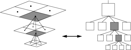
Figure 1. Graded tree data structure (“quadtree”), after [30].

We denote by root the basis of the tree. In two space dimensions, a parent node has four sons, and the sons of the same parent are called brothers. A node without sons is called a leaf. A given node has $s^{\prime}=2$ nearest neighbors in each direction, called nearest cousins, needed for the computation of the fluxes of leaves; if these nearest cousins do not exist, we create them as virtual leaves. Brothers are also considered nearest cousins. Figure 1 illustrates the graded tree structure. The leaves of the tree are the control volumes from which we form the adaptive mesh. Here, the property of the tree being graded means that grid refinement and coarsening is governed by that two neighboring control volumes cannot differ by more than one level in the tree. This is equivalent with the notion of ”one-irregular rule” (see e.g., [28, 29]). We denote by $\Lambda$ the set of indices of existing nodes, by $\mathcal{L}(\Lambda)$ the restriction of $\Lambda$ to the leaves, and by $\Lambda_{l}$ the restriction of $\Lambda$ to a multiresolution level $l$, $0\leq l\leq L$. We denote by $\bar{\mathbf{w}}_{i,j,l}=(\bar{u}_{i,j,l},\bar{v}_{i,j,l})$ the vector of cell averages for both components of the solution (and the obvious simplification $\bar{\mathbf{w}}_{i,j,l}=\bar{u}_{i,j,l}$ for a single-species problem) located at spatial position $(i,j)$ at level $l$, and by $\smash{\bar{\mathbf{W}}_{l}}$ the set of cell averages for all nodes at level $l$. To estimate the cell averages of a level $l$ from those of the next finer level $l+1$, we use the projection operator $P_{l+1\to l}$, which is exact, unique, and in our case is defined by

$$\bar{\mathbf{w}}_{i,j,l}=\frac{1}{4}\sum_{e_{1},e_{2}\in\{0,1\}}\bar{\mathbf{w}}_{2i+e_{1},2j+e_{2},l+1}.$$ (4.1)

To estimate the cell averages of a level $l+1$ from those of level $l$, we employ the prediction operator $P_{l\to l+1}$, which provides an approximation $\hat{\mathbf{w}}$ by interpolation of $\smash{\bar{\mathbf{W}}_{l}}$ at level $l+1$. This operator is local in the sense that the interpolation for a son is made from the cell averages of its parent and the $s$ nearest cousins of its parent; and it is consistent with the projection in the sense that it is conservative with respect to the coarse grid cell averages or equivalently, $P_{l+1\to l}\circ P_{l\to l+1}=\mathrm{Id}$. For a regular grid structure in two dimensions, we use a polynomial interpolation introduced in [2]:

$$\hat{\mathbf{w}}_{2i+e_{1},2j+e_{2},l+1}=\bar{\mathbf{w}}_{i,j,l}-(-1)^{e_{1}}Q_{x}-(-1)^{e_{2}}Q_{y}+(-1)^{e_{1}e_{2}}Q_{xy},\quad e_{1},e_{2}\in\{0,1\},$$ (4.2)

where

$$\begin{split}Q_{x}&:=\sum_{n=1}^{s}\tilde{\gamma}_{n}(\bar{\mathbf{w}}_{i+n,j,l}-\bar{\mathbf{w}}_{i-n,j,l}),\quad Q_{y}:=\sum_{p=1}^{s}\tilde{\gamma}_{p}(\bar{\mathbf{w}}_{i,j+p,l}-\bar{\mathbf{w}}_{i,j-p,l}),\\ Q_{xy}&:=\sum_{n=1}^{s}\tilde{\gamma}_{n}\sum_{p=1}^{s}\tilde{\gamma}_{p}(\bar{\mathbf{w}}_{i+n,j+p,l}-\bar{\mathbf{w}}_{i+n,j-p,l}-\bar{\mathbf{w}}_{i-n,j+p,l}+\bar{\mathbf{w}}_{i-n,j-p,l}).\end{split}$$ (4.3)

The chosen accuracy order of the multiresolution method for our cases is $r=s+1=3$, where $s$ is the number of required nearest uncles for each spatial direction. The corresponding coefficients are $\tilde{\gamma}_{1}=\smash{-\frac{22}{128}}$ and $\tilde{\gamma}_{2}=\smash{\frac{3}{128}}$. Nevertheless, one may select here an arbitrarily higher order of accuracy.

As stated before, the adaptive grid consists in the set of leaves $\mathcal{L}(\Lambda)$, which forms a partition of the computational domain $\Omega$.

A detail is the difference between the exact and the predicted value

$$\bar{d}^{u}_{i,j,l}:=\bar{u}_{i,j,l}-\hat{u}_{i,j,l},\quad\bar{d}^{v}_{i,j,l}:=\bar{v}_{i,j,l}-\hat{v}_{i,j,l}.$$

For multicomponent solutions, there are many possible definitions of a scalar detail $\smash{\bar{d}_{i,j,l}}$ that is calculated from the details of the components (in our case, $\smash{\bar{d}^{u}_{i,j,l}}$ and $\smash{\bar{d}^{v}_{i,j,l}}$), depending mainly on the nature of the problem. Roussel and Schneider [36] utilize the Euclidian norm of the details, $\smash{\bar{d}_{i,j,l}=((\bar{d}^{u}_{i,j,l})^{2}+(\bar{d}^{v}_{i,j,l})^{2})^{1/2}}$. In our case, given the nature of our problems, we could simply select one component $\smash{\bar{d}_{i,j,l}=\bar{d}^{u}_{i,j,l}}$, as was done by Sjögreen [39] for the compressible Euler equations, but in order to guarantee that the computations of the refinement and coarsening procedures are always on the safe side, in the sense that we always prefer to keep a node with a detail pair containing at least one value over the threshold

$$\varepsilon_{l}=2^{2(l-L)}\varepsilon,$$ (4.4)

we will use $\smash{\bar{d}_{i,j,l}=\min\{\bar{d}^{u}_{i,j,l},\bar{d}^{v}_{i,j,l}\}}$ and $\smash{\bar{d}_{i,j,l}=\max\{\bar{d}^{u}_{i,j,l},\bar{d}^{v}_{i,j,l}\}}$ for the refinement and coarsening procedures (see details in Algorithm 7.1), respectively, similar to Harten’s choice [19] for the Euler equations of gas dynamics.

Since a parent has four sons, the consistency property of the prediction operator implies that knowledge of the cell average values of the four sons is equivalent to that of the cell average value of the parent node and three independent details. Repeating this operation recursively on $L$ levels, we get the multiresolution transform on the cell average values $\smash{\bar{\mathbf{M}}:\bar{\mathbf{W}}_{L}\mapsto(\bar{D}_{L},\ldots,\bar{D}_{1},\bar{\mathbf{W}}_{0})}$, where $\smash{\bar{D}_{l}=(\bar{d}_{i,j,l})_{(i,j)}}$. This means that knowledge of the cell averages of all leaves is equivalent to that of the cell average value of the root and of the details of all nodes of the tree.

After thresholding, i.e., removing nodes where the detail is below the prescribed tolerance $|\bar{d}_{i,j,l}|<\varepsilon_{l}$, where $\varepsilon_{l}$ is given by (4.4); a safety zone is added to the tree, which means that one finer level is added to the tree in all possible nodes without violating the graded tree data structure. This is done by splitting each leaf into four new leaves in such a way that the new tree remains graded. This device, which was proposed e.g. in [19, 35], ensures that the graded tree will represent adequately the solution in the next time step, and depends strongly on the assumption of finite propagation speed of sharp fronts.

Now, assume that the tree has only two levels $l$ and $l+1$ (straightforwardly extensible to an arbitrarily larger tree). To ensure conservativity of the scheme, we compute only the fluxes at level $l+1$ and we set the ingoing flux on the leaf at level $l$ equal to the sum of the outgoing fluxes on the leaves of level $l+1$ (see Figure 2)

$$F_{(i+1,j,l)\to(i,j,l)}=F_{(2i+1,2j,l+1)\to(2i+2,2j,l+1)}+F_{(2i+1,2j+1,l+1)\to(2i+2,2j+1,l+1)}.$$ (4.5)

This choice decreases the number of costly flux evaluations without loosing the conservativity in the flux computation, and this presents a real advantage when using a graded tree structure, see e.g. [35]. This advantage is lost for a non-graded tree structure, in which case these data (fluxes for leaves on an immediately finer level) are not always available.

Figure 2. Conservative flux computation for coarser levels.

It is important to remark that in the case of systems, since we are dealing with reaction-diffusion systems where species tend to attract each other, we manage the multiresolution framework and the data structure as one unified mesh with two components per control volume. This means that we construct only one graded tree and apply only one thresholding strategy for both species; however, there are other cases where it is preferable to organize the different species in separate adaptive meshes, for example when the species segregate spatially, as in systems of conservation laws modelling traffic flow and polydisperse sedimentation [5].

5. Error analysis of the adaptive multiresolution scheme

Using the main properties of the reference finite volume scheme on a uniform grid at the finest level $L$, such as the contraction property in $L^{1}$ norm, CFL stability condition and order of approximation in space, in [13, 35], the authors decompose the global error between the cell average values of the exact solution vector at the level $L$, denoted by $\bar{\mathbf{w}}^{L}_{\mathrm{ex}}=(\bar{u}^{L}_{\mathrm{ex}},\bar{v}^{L}_{\mathrm{ex}})$, and those of the multiresolution computation with a maximal level $L$, denoted by $\bar{\mathbf{w}}^{L}_{\mathrm{MR}}$, into two errors

$$\bigl{\|}\bar{\mathbf{w}}^{L}_{\mathrm{ex}}-\bar{\mathbf{w}}^{L}_{\mathrm{MR}}\bigr{\|}\leq\bigl{\|}\bar{\mathbf{w}}^{L}_{\mathrm{ex}}-\bar{\mathbf{w}}^{L}_{\mathrm{FV}}\bigr{\|}+\bigl{\|}\bar{\mathbf{w}}^{L}_{\mathrm{FV}}-\bar{\mathbf{w}}^{L}_{\mathrm{MR}}\bigr{\|}.$$ (5.1)

The first error on the right-hand side, called discretization error, is the one of the reference finite volume scheme on a uniform grid at the finest level $L$. In many circumstances (see e.g. [8, 13]), this error can be bounded by

$$\bigl{\|}\bar{\mathbf{w}}^{L}_{\mathrm{ex}}-\bar{\mathbf{w}}^{L}_{\mathrm{FV}}\bigr{\|}\leq C_{1}2^{-\tilde{\alpha}L},\quad C_{1}>0,$$ (5.2)

where $\tilde{\alpha}$ is the convergence order of the finite volume scheme. Based on preliminary numerical experiments (obtained in a similar fashion as in [8]), for our examples we obtain the approximate value $\tilde{\alpha}=2.18$.

For the second error, called perturbation error, in [13] the authors assume that the details on a level $l$ are deleted when they are smaller than a prescribed tolerance $\varepsilon_{l}$. Under this assumption, they show that if the discrete time evolution operator is contractive in the chosen norm, and if the tolerance $\varepsilon_{l}$ at the level $l$ is given by (4.4), then the perturbation error accumulates in time and satisfies

$$\bigl{\|}\bar{\mathbf{w}}^{L}_{\mathrm{FV}}-\bar{\mathbf{w}}^{L}_{\mathrm{MR}}\bigr{\|}\leq C_{2}n\varepsilon,\quad C_{2}>0,$$ (5.3)

where $n$ denotes the number of time steps. At a fixed time $T=n\Delta t$, this gives

$$\bigl{\|}\bar{\mathbf{w}}^{L}_{\mathrm{FV}}-\bar{\mathbf{w}}^{L}_{\mathrm{MR}}\bigr{\|}\leq C_{2}\frac{T}{\Delta t}\varepsilon,\quad C_{2}>0.$$

Motivated by their analysis, and according to the global CFL condition (3.4) of the reference finite volume scheme defined for the discretization of Model 2, we have

$$\Delta t\leqslant\frac{\widetilde{\Delta x}{}^{2}}{\|f_{u}\|_{\infty}+\|f_{v}\|_{\infty}+\|g_{u}\|_{\infty}+\|g_{v}\|_{\infty}+\widetilde{\Delta x}4d(\|A^{\prime}\|_{\infty}+\|B^{\prime}\|_{\infty})}.$$

If we write $\smash{\widetilde{\Delta x}=\sqrt{|\Omega|}2^{-L}}$, this yields

$$\Delta t=C_{3}\frac{|\Omega|2^{-2L}}{\|f_{u}\|_{\infty}+\|f_{v}\|_{\infty}+\|g_{u}\|_{\infty}+\|g_{v}\|_{\infty}+\sqrt{|\Omega|}2^{-L}4d(\|A^{\prime}\|_{\infty}+\|B^{\prime}\|_{\infty})},\quad 0<C_{3}\leqslant 1.$$

The main idea of the adaptive multiresolution scheme is to perturb the solution given by a finite volume scheme on a uniform discretization (reference mesh) in such a way that the total error, i.e., the error between the exact solution and the adaptive solution that is projected to the reference fine mesh, is of the same order as the discretization error. For this purpose, one has to balance the discretization error and the perturbation error. With this idea in mind, it is possible to derive in a similar fashion the optimal choice for the threshold parameter $\varepsilon$ for the adaptive multiresolution scheme.

As in [8], we need that $\varepsilon\propto 2^{-\tilde{\alpha}L}$ or

$$\varepsilon|\Omega|2^{2L}\Bigl{(}\|f_{u}\|_{\infty}+\|f_{v}\|_{\infty}+\|g_{u}\|_{\infty}+\|g_{v}\|_{\infty}+\sqrt{|\Omega|}2^{-L}4d\bigl{(}\|A^{\prime}\|_{\infty}+\|B^{\prime}\|_{\infty}\bigr{)}\Bigr{)}\propto 2^{-\tilde{\alpha}L}.$$

In this way, for the numerical computations of Model 2, we may set the so-called reference tolerance $\varepsilon_{\mathrm{R}}$ to

$$\varepsilon_{\mathrm{R}}=C\frac{2^{-(\tilde{\alpha}+2)L}}{|\Omega|(\|f_{u}\|_{\infty}+\|f_{v}\|_{\infty}+\|g_{u}\|_{\infty}+\|g_{v}\|_{\infty})+|\Omega|^{3/2}2^{L}\,4d(\|A^{\prime}\|_{\infty}+\|B^{\prime}\|_{\infty})}.$$ (5.4)

Analogously, for Model 3, the reference tolerance may be set to

$$\varepsilon_{\mathrm{R}} =C\frac{2^{-(\tilde{\alpha}_{1}+2)L}}{|\Omega|(\|h_{u}\|_{\infty}+\|h_{v}\|_{\infty}+\|g^{\prime}\|_{\infty})+|\Omega|^{3/2}2^{L}\,4d(\sigma+\|\chi^{\prime}\|_{\infty})},$$ (5.5)

where $\tilde{\alpha}_{1}$ is a value of the convergence rate for Model 3.

Note that all the $L^{\infty}$ norms in (5.4) and (5.5) are computed numerically. To determine an acceptable value for the factor $C$ (which, of course, depends on $T$, $C_{1}$, $C_{2}$ and $C_{3}$), a series of computations with different tolerances are needed in each case, prior to final computations. Essentially, we select the largest available candidate value for $C$ such that the same order of accuracy (same slopes for the error computation) as that of the reference finite volume scheme is maintained. This procedure basically generalizes the treatment in [7] of spatially one-dimensional strongly degenerate parabolic equations. In [15] the authors prove for scalar, one-dimensional, nonlinear conservation laws, that the threshold error is stable in the sense that the constant $C$ is uniformly bounded and, in particular, does not depend on the threshold value $\varepsilon_{\mathrm{R}}$, the number of refinement levels $L$ and the number of time steps $n$. In our case, even when a rigorous proof is still missing for the systems considered in the present work, from the previous deduction we see a similar behavior for $C$.

We also mention that as in previous works [7, 8, 13], here the reference tolerance remains fixed for all times, though it is certainly possible to recompute the reference tolerance at each time step.

6. Local time stepping

We utilize a version of the locally varying time stepping strategy advanced by Müller and Stiriba [31], and summarize here its principles. The basic idea is to enforce a local CFL condition by using the same CFL number for all levels, and the strategy consists in evolving all leaves on level $l$ using the local time step

$$\Delta t_{l}=2^{L-l}\Delta t,\quad l=L-1,\ldots,0,$$ (6.1)

where $\Delta t=\Delta t_{L}$ corresponds to the time step on the finest level $L$. This strategy allows to increase the time step for the major part of the adaptive mesh without violating the CFL stability condition.

Clearly, portions of the solution lying on different resolution levels need to be synchronized to obtain a conservative scheme. This will be achieved after $2^{l}$ time steps using $\Delta t_{l}$: all leaves forming the adaptive mesh are synchronized in time, so one time step with $\Delta t_{0}$ is equivalent to $2^{L}$ intermediate time steps with $\Delta t_{L}$. In order to additionally save computational effort, we update the tree structure (refinement and coarsening) only each odd intermediate time step $1,3,\ldots,2^{L}-1$ (as suggested in [1]), and furthermore, the projection and prediction operators are performed only on the levels occupied by the leaves of the current tree, i.e., we do not update the tree structure by prediction from the root cell, but from the coarsest leaves (we refer to this as partial grid adaptation). For the rest of the intermediate time steps, we use the current tree structure. Notice that the updating of the tree is still done in each global time step. For the sake of synchronization and conservativity of the flux computation, for coarse levels (levels without leaves), we employ the same fluxes ($\smash{\bar{\mathcal{D}}_{ij,l}}$ and $\smash{\bar{f}_{ij,l}}$) computed in the previous intermediate time step, because the cell averages on these levels are the same that in the previous intermediate time step. Only for finer levels (levels containing leaves), we compute fluxes, and do so in the following way: if there is a leaf at the corresponding cell edge and at the same resolution level $l$, we simply perform a flux computation using the brother leaves, and the virtual leaves at the same level if necessary; and if there is a leaf at the corresponding cell edge but on a finer resolution level $l+1$ (in this case we refer to this edge as an interface edge), the flux will be determined as in (4.5), that is, we compute the fluxes at a level $l+1$ on the same edge, and we set the ingoing flux on the corresponding edge at level $l$ equal to the sum of the outgoing fluxes of the son cells of level $l+1$ (for the same edge). We recall that the graded tree structure ensures that two neighboring control volumes of the adaptive mesh do not differ by more than one resolution level, which is equivalent to the satisfaction of the one-irregular rule. In order to always have at hand the computed fluxes as in (4.5), we need to perform the locally varying time stepping recursively from fine to coarse levels. If at any instance of the procedure there is a missing value, we can project the value from the sons nodes or we can predict this value from the parent nodes. For illustrative purposes, we give an example of an interior first-order flux calculation for Model 2, to complete a full macro time step, by the following algorithm (we show only the flux calculation for $(i,j,l)\to(i+1,j,l)$ and $(i,j,l)\to(i,j+1,l)$ since the other fluxes are obtained analogously):

Algorithm 6.1 (Locally varying intermediate time stepping).

1. Grid adaptation (provided the former sets of leaves and virtual leaves).

2. do $k=1,\ldots,2^{L}$ (and therefore the local time steps are $n+2^{-L},n+2\cdot 2^{-L},n+3\cdot 2^{-L},\ldots,n+1$)

   1. Synchronization:

   2. do $l=L,\ldots,1$

      • do $i=1,\dots,|\tilde{\Lambda}|_{x}(l)$, $j=1,\dots,|\tilde{\Lambda}|_{y}(l)$

        • if $1\leqslant l\leqslant\tilde{l}_{k-1}$ then

          • if $(i,j,l)$ is a virtual leaf then

            • ${\displaystyle\bar{F}^{n+k2^{-L}}_{(i,j,l)\to(i+1,j,l)}\leftarrow\bar{F}^{n+(k-1)2^{-L}}_{(i,j,l)\to(i+1,j,l)}\vphantom{\int}}$

            • ${\displaystyle\bar{f}_{ij,l}^{n+k2^{-L}}\leftarrow\bar{f}_{ij,l}^{n+(k-1)2^{-L}},\quad\bar{g}_{ij,l}^{n+k2^{-L}}\leftarrow\bar{g}_{ij,l}^{n+(k-1)2^{-L}}\vphantom{\int}}$

          • endif

        • else

          • if $(i,j,l)$ is a leaf then

            • ${\displaystyle\bar{f}_{ij,l}^{n+k2^{-L}}\leftarrow f\bigl{(}\bar{u}_{ij,l}^{n+k2^{-L}},\bar{v}_{ij,l}^{n+k2^{-L}}\bigr{)},\quad\bar{g}_{ij,l}^{n+k2^{-L}}\leftarrow g\bigl{(}\bar{u}_{ij,l}^{n+k2^{-L}},\bar{v}_{ij,l}^{n+k2^{-L}}\bigr{)}\vphantom{\int}}$

            • if $(i+1,j,l)$ is a leaf or $(i,j+1,l)$ is a leaf then compute fluxes by

            • $\quad{\displaystyle\bar{F}_{(i,j,l)\to(i+1,j,l)}\leftarrow-\frac{1}{h(l)}\bigl{(}A(\bar{u}_{i+1,j,l})-A(\bar{u}_{i,j,l})\bigr{)}\vphantom{\int\limits_{x}^{x}}}$

            • $\quad{\displaystyle\bar{F}_{(i,j,l)\to(i,j+1,l)}\leftarrow-\frac{1}{h(l)}\bigl{(}A(\bar{u}_{i,j+1,l})-A(\bar{u}_{i,j,l})\bigr{)}\vphantom{\int\limits_{x}^{x}}}$

            • endif

            • if $(2i+2,2j,l+1)$, $(2i+2,2j+1,l+1)$ are leaves (interface edges) then compute fluxes by

            • $\quad{\displaystyle\vphantom{\int}\bar{F}_{(i,j,l)\to(i+1,j,l)}\leftarrow\bar{F}_{(2i+2,2j,l+1)\to(2i+1,2j,l+1)}+\bar{F}_{(2i+2,2j+1,l+1)\to(2i+1,2j+1,l+1)}\vphantom{\int}}$

            • $\quad{\displaystyle\vphantom{\int}\bar{F}_{(i,j,l)\to(i,j+1,l)}\leftarrow\bar{F}_{(2i,2j+2,l+1)\to(2i,2j+1,l+1)}+\bar{F}_{(2i+1,2j+2,l+1)\to(2i+1,2j+1,l+1)}\vphantom{\int}}$

            • endif

          • endif

        • endif

      • enddo

   3. enddo

   4. Time evolution:

   5. do $l=1,\ldots,L$, $i=1,\dots,|\tilde{\Lambda}|_{x}(l)$, $j=1,\dots,|\tilde{\Lambda}|_{y}(l)$

      • if $1\leqslant l\leqslant\tilde{l}_{k-1}$ then there is no evolution:

        • ${\displaystyle\bar{u}_{ij,l}^{n+(k+1)2^{-L}}\leftarrow\bar{u}_{ij,l}^{n+k2^{-L}},\quad\bar{v}_{ij,l}^{n+(k+1)2^{-L}}\leftarrow\bar{v}_{ij,l}^{n+k2^{-L}}}$

      • else

        • Interior marching formula only for the leaves $(i,j,l)$:

        • ${\displaystyle\bar{u}_{ij,l}^{n+(k+1)2^{-L}}\leftarrow\bar{u}_{ij,l}^{n+k2^{-L}}+\gamma\Delta t_{l}\bar{f}_{ij,l}^{n+k2^{-L}}+\Delta t_{l}\bar{\mathcal{D}}_{ij,l}\bigl{(}\mathcal{S}\bigl{(}\bar{u}_{ij,l}^{n+k2^{-L}}\bigr{)},h(l)\bigr{)}\vphantom{\int}}$

        • ${\displaystyle\bar{v}_{ij,l}^{n+(k+1)2^{-L}}\leftarrow\bar{v}_{ij,l}^{n+k2^{-L}}+\gamma\Delta t_{l}\bar{g}_{ij,l}^{n+k2^{-L}}+d\Delta t_{l}\bar{\mathcal{D}}_{ij,l}\bigl{(}\mathcal{S}\bigl{(}\bar{v}_{ij,l}^{n+k2^{-L}}\bigr{)},h(l)\bigr{)}}$

      • endif

   6. enddo

   7. Partial grid adaptation each odd intermediate time step:

   8. do $l=L,\ldots,\tilde{l}_{k}+1$

      • Projection from the leaves.

      enddo

   9. do $l=\tilde{l}_{k},\ldots,L$

      • Thresholding, prediction, and addition of the safety zone.

      enddo

3. enddo

Here, $\tilde{l}_{k}$ denotes the coarsest level containing leaves in the intermediate step $k$ (as introduced in [31]), $h(l)$ is the mesh size on level $l$, and $|\tilde{\Lambda}|_{z}(l)$ is the size of the set formed by leaves and virtual leaves per resolution level $l$ in the direction $z$. The interior marching formula is the modified marching formula (3.3) for Model 2, for the intermediate time steps $k=1,\ldots,2^{L}$, for the leaf in the position $(i,j)$ at level $l$.

Our scheme is formulated for a first-order, explicit Euler time discretization. Generalizations for higher order schemes are given in [31] for Crank-Nicolson schemes and in [16] for Runge-Kutta schemes, respectively.

7. Algorithm implementation

Now we give a brief description of the multiresolution procedure used to solve the test problems.

Algorithm 7.1 (Multiresolution procedure).

1. Initialization of parameters.

2. Creation of the initial graded tree structure:

   1. Create the root of the tree and compute its cell average value.

   2. Split the cell, compute the cell average values in the sons and compute the corresponding details.

   3. Apply the thresholding strategy for the splitting of the new sons: If $d_{i,j,l}>\varepsilon_{l}$ then split the son (here we use $\smash{d_{l}=\min\{d_{l}^{u},d_{l}^{v}\}}$).

   4. Repeat this until all sons have details below the required tolerance $\varepsilon_{l}$.

3. do $n=1,\dots,total\_time\_steps$

   1. Determination of the leaves and virtual leaves sets.

   2. Time evolution with global time step: Compute the discretized divergence operator for all the leaves.

   3. Updating the tree structure:

      • Recalculate the values on the nodes and the virtual nodes by projection from the leaves. Compute the details for all positions $(\cdot,\cdot,l)$ for $l\geqslant\tilde{l}_{k}$.

        if $|\bar{d}_{i,j,l}|<\varepsilon_{l}$ (here we use $d_{l}=\max(d_{l}^{u},d_{l}^{v})$) in a node and in its brothers then the cell and its brothers are deletable.

        endif

      • if some node and all its sons are deletable and the sons are leaves without virtual sons, then delete sons (coarsening).

        • if this node has no sons and it is not deletable and it is not at level $l=L$, then create sons (refinement).

        • endif

        endif

      • Update the values in the new sons by prediction operator from the former leaves.

4. enddo

5. Output: Save meshes, leaves and cell averages.

Here $total\_time\_steps$ stands for the total time steps needed to reach $T_{\text{final}}$ using $\Delta t$ as the maximum time step allowed by the CFL condition using the finest space step.

When using a locally varying time stepping, replace step (3b) by the new step

1. do $n=1,\dots,total\_time\_steps$

   1. Determination of the leaves and virtual leaves sets.

   2. Time evolution with local time stepping: Compute the discretized divergence operator for all the leaves and virtual leaves

   3. do $k=1,\dots,2^{L}$ ($k$ counts intermediate time steps)

      • Compute the intermediate time steps depending on the position of the corresponding leaf as explained in Section 6.

      • if $k$ is odd then update the tree structure:

        • Recalculate the values on the nodes and the virtual nodes by projection from the leaves. Compute the details in the whole tree.

          if $|\bar{d}_{i,j,l}|<\varepsilon_{l}$ (here we use $d_{l}=\max(d_{l}^{u},d_{l}^{v})$) in a node and in its brothers then the cell and its brothers are deletable.

          endif

        • if some node and all its sons are deletable and the sons are leaves without virtual sons, then delete sons (coarsening).

          • if this node has no sons and it is not deletable and it is not at level $l=L$, then create sons (refinement).

          • endif

          endif

        • Update the values in the new sons by prediction operator from the former leaves.

      • endif

   4. enddo

   5. (Now, after $2^{L}$ intermediate steps, all nodes are synchronized.)

2. enddo

Here $total\_time\_steps$ for the new step stands for the total time steps needed to reach $T_{\text{final}}$, with $\Delta t_{0}$ as the maximum time step allowed by the CFL condition using the coarsest space step.

Notice that with such a process, we obtain high-order approximation in the smooth regions and mesh refinement near discontinuities as a consequence of the polynomial accuracy in the multiresolution prediction operator, even if the reference finite volume scheme is low-order accurate.

Bihari and Harten [2] use the following quantity, which we call data compression rate,

$$\eta:=\frac{N_{Lx}N_{Ly}}{N_{Lx}N_{Ly}/2^{2L}+|\mathcal{L}(\Lambda)|},$$ (7.1)

to measure the possible improvement in data compression, whose feasibility in turn strongly depends on a smart implementation to navigate inside the tree, see for example [35]. Here, $N_{Lx}N_{Ly}$ is the number of cells in the finest grid, and $|\mathcal{L}(\Lambda)|$ is the size of the set of leaves. We measure the speed-up between the CPU time of the numerical solution obtained by the FV method and the CPU time of the numerical solution obtained by the multiresolution method: $V=(\mathrm{CPU\,time})_{\mathrm{FV}}/(\mathrm{CPU\,time})_{\mathrm{MR}}$.

To measure errors between a reference solution $u$ and an approximate solution $u_{MR}$ obtained using multiresolution, we will use $L^{p}$-errors: $e_{p}=\smash{\|u^{n}-u^{n}_{\mathrm{MR}}\|_{p}}$, $p=1,2,\infty$, where

$$e_{\infty}=\max_{1\leq i\leq N_{Lx},1\leq j\leq N_{Ly}}\bigl{|}u^{n}_{i,j}-{u^{n}_{\mathrm{MR}}}_{i,j,L}\bigr{|},$$

$$e_{p}=\left(\frac{1}{N_{Lx}N_{Ly}}\sum_{i=1}^{N_{Lx}}\sum_{j=1}^{N_{Lx}}\bigl{|}u^{n}_{i,j}-{u^{n}_{\mathrm{MR}}}_{i,j,L}\bigr{|}^{p}\right)^{1/p},\quad p=1,2.$$

Here $\smash{{u^{n}_{\mathrm{MR}}}_{i,j,L}}$ is the value on the finest level $L$ obtained by prediction from the corresponding leaf.

8. Numerical results

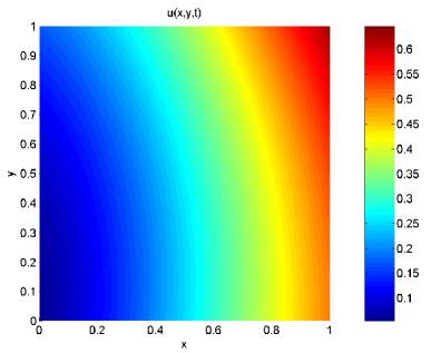
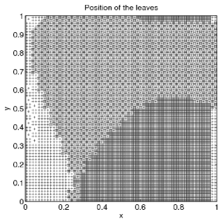
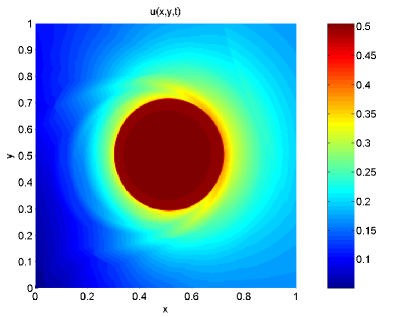
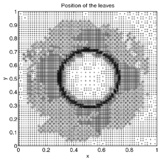
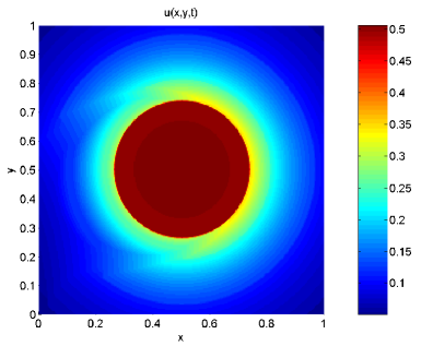
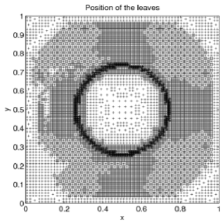
Figure 3. Example 1 (single-species model): Numerical solution (left) and leaves (right) of the corresponding tree data structure at times $t=0$ (top), $t=0.5$ (middle) and $t=3$ (bottom).

(a)	(b)	(c)

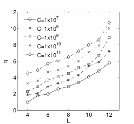
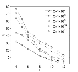
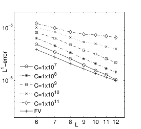
Figure 4. Example 1 (single-species model): (a) data compression rate $\eta$, (b) speed-up factor $V$ and (c) $L^{1}$-errors for different levels $L$ and values of $C$. The simulated time is $t=0$.

8.1. Example 1: Single-species model

For this example, we consider (2.1) with a strongly degenerate diffusion term (2.3), where we choose $D:=1$ and $u_{\mathrm{c}}:=0.5$, a square domain $\Omega=[0,1]^{2}$, and the function $f(u,\mathbf{x})$ given by (2.2). Figure 3 displays the numerical solution starting from the smoothly varying initial function

$$u_{0}(x,y)=0.5\big{(}1+\sin(1.1(x-\cos(0.7y))\big{)}\cos\bigl{(}0.5(y-\sin(1.3x))\bigr{)}.$$

We choose a maximal resolution level of $N_{L}=256^{2}=65536$ control volumes on the finest grid. Figure 4 illustrates how the factor $C$ in (5.4) is selected in our case as the optimal value from a finite selection of test values (each value giving a different value for the reference tolerance (5.4) $\varepsilon_{\mathrm{R}}$). Figures 4 (a) and (b) indicate that for all displayed levels, the multiresolution procedure is in every case (for different values of $C$) cheaper (in terms of both acceleration and memory savings) than the corresponding reference FV computation on the finest grid. Figure 4 (c) indicates that the computations obtained using $C=1.0\times 10^{9}$ (and hence $\varepsilon_{\mathrm{R}}=9.43\times 10^{-4}$) are sufficiently accurate, in the sense that with these choices, we keep the same slope for the $L^{1}$-error as the FV calculations while increasing $V$ and $\eta$. We remark that here, as in previous works that use similar methods (see e.g. [13]), there actually exists a range of threshold parameters that preserve the same slope for errors with respect to reference solution, for which $C=1.0\times 10^{9}$ is an average value. Here, we compute errors using a reference FV solution on a fine grid with $N_{L}=2048^{2}=4194304$ control volumes. (Here and in all other examples, we calculate errors in the approximate sense with respect to a reference solution.)

8.2. Examples 2 and 3: Interaction between two flame balls

We study (2.4) as a dimensionless model for the interaction between two flame balls of different sizes. We consider a square domain $\Omega=[-30,30]^{2}$ and that the walls are sufficiently far from the flame balls so that their influence is negligible. Physical parameters characterizing the gaseous mixture and the combustion process are chosen as in [36, 37]. We use the parameters $\alpha=0.64$ and $\beta=10$. The initial data is given by $u(x,y,0)=u_{0}(r_{1},r_{2}),\ v(x,y,0)=v_{0}(r_{1},r_{2})$ with $r_{1}^{2}=(x-x_{1})^{2}+y^{2},\ r_{2}^{2}=(x-x_{2})^{2}+y^{2}$, where

$$u_{0}(r_{1},r_{2}) :=\begin{cases}1&\text{if $r_{1}<a$ or $r_{2}<b$,}\\ \max\bigl{\{}\exp(1-r_{1}/a),\exp(1-r_{2}/b)\bigr{\}}&\text{otherwise,}\end{cases}\quad v_{0}(r_{1},r_{2}):=1-u_{0}(r_{1},r_{2}).$$ (8.1)

In Example 2, we simulate the process without radiation, i.e., $\rho=0$ and hence $S(u)=0$. We set the Lewis number to $\mathrm{Le}=1$. Here $x_{1}=-7.5$, $x_{2}=7.5$ and $a=1.8$, $b=2.5$ are the respective $x-$position and initial radii of the two flame balls. This choice ensures that there is no interaction between the two flame balls at $t=0$ and that there is no extinction of the flame balls. We simulate the process until $t=10$, and Figure 5 shows from left to right the temperature and reaction rate configuration obtained using the fully adaptive multiresolution scheme, and the position of the dynamic graded tree leaves, which form the corresponding adaptive mesh. The different times correspond from the top to the bottom to: before ($t=2$), during ($t=4$) and after ($t=10$) direct interaction between the two flame balls, when the balls tend to create a new circular flame structure. We choose the following multiresolution parameters: the maximal resolution level $L=10$ corresponding to $N_{L}=512^{2}=262144$ control volumes in the finest grid, and the reference tolerance $\varepsilon_{\mathrm{R}}=4.94\times 10^{-3}$.

For comparison purposes, we introduce the global chemical reaction rate

$$R(t):=\iint_{\Omega}f(u,v)\,dx\,dy.$$

Errors in different norms, reaction rates, information on data compression and speed-up rate for different methods at three different times are depicted in Table 1. Due to the particular shape of solutions, which is nearly constant away from the combustion front, by using multiresolution, one can obtain very high rates of data compression, speed-up and low errors.

In Example 3, we simulate the case with radiation, i.e. we use (2.6) and (2.7), where $\rho=0.05$ and $\mathrm{Le}=0.3$. Now $x_{1}=-5$, $x_{2}=5$ and $a=0.5$, $b=1$ are the respective $x-$position and initial radii of the two flame balls. We simulate the process until $t=10$ and Figures 6 and 7 show the scenario for this case. First, the balls grow spherically, tend to create a new flame structure, and then their fronts tend to extinguish when they touch each other, while the radiation effect causes the entire flame front to split. Here the maximal resolution level is set to $L=10$ corresponding to $N_{L}=512^{2}=262144$ control volumes in the finest grid, and the reference tolerance is $\varepsilon_{\mathrm{R}}=7.43\times 10^{-3}$.

Notice that the multiresolution procedure automatically detects the higher gradient regions and uses this information to adaptively represent the solution by the refinement and coarsening of the mesh, i.e., by the adaptive addition and removal of control volumes on these areas.

The $L^{1}$, $L^{2}$ and $L^{\infty}$ errors between the numerical solution obtained by our multiresolution scheme for different multiresolution levels $L$ and the reference solution (obtained by finite volume approximation in a uniform fine grid with $2^{2\cdot 14}$ control volumes) for Example 2 are depicted in Figure 8 (c) and (d). The slopes indicate a rate of convergence slightly better than two.

For Example 3, we apply the locally varying time stepping (LTS) strategy detailed in Section 6. We choose the maximum CFL number allowed by (3.4), which is $\mathsf{CFL}_{0}=1$ for the coarsest level. For the remaining levels we use $\mathsf{CFL}_{l}=2^{l}\mathsf{CFL}_{0}$, which means that we perform each macro time step with $\Delta t=\Delta t_{0}=2^{L}\Delta t_{L}$ as given by (6.1).

In Figure 9 we compare speed-up, data compression rate and total reaction rate for the finite volume reference scheme, the multiresolution scheme with global time step, and the multiresolution method with level-dependent time stepping. Notice that with LTS, the speed-up rate is approximately doubled for all times, while the compression rate and the total reaction rate remain of the same order as the multiresolution computation with global time step.

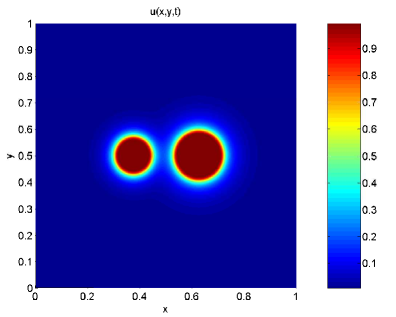
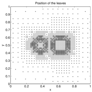
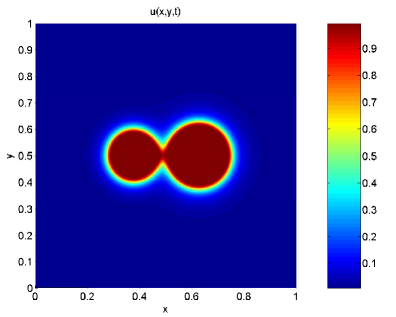
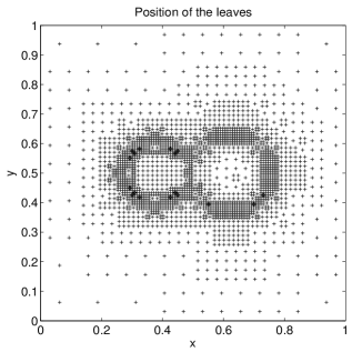
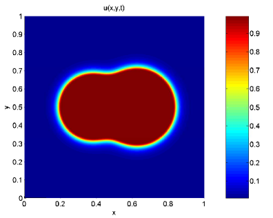
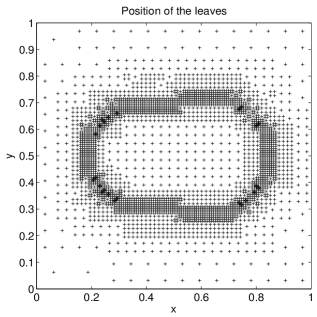
Figure 5. Example 2 (interaction of two flame balls without radiation): Numerical solution for species $u$ (left) and leaves of the corresponding tree data structure (right) at times $t=2$ (top), $t=4$ (middle) and $t=10$ (bottom).

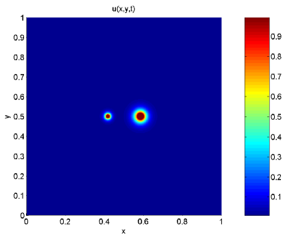
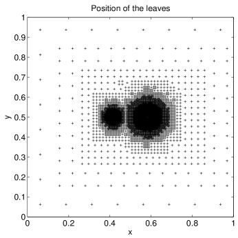
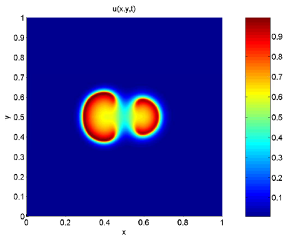
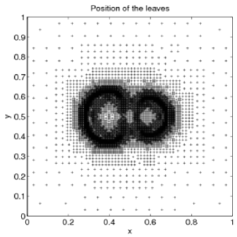
Figure 6. Example 3 (interaction of two flame balls with radiation): Numerical solution for species $u$ (left) and and leaves of the corresponding tree (right) at times $t=0$ (top) and $t=5$ (bottom).

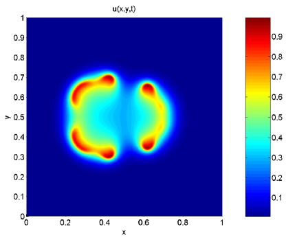
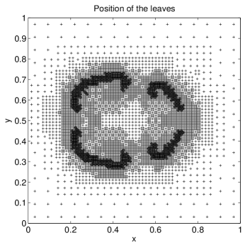
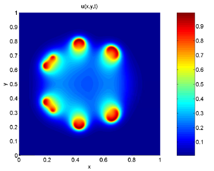
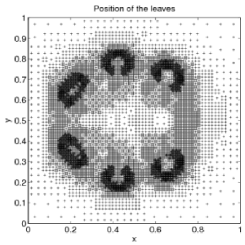
Figure 7. Example 3 (interaction of two flame balls with radiation): Numerical solution for species $u$ and leaves of the corresponding tree (right) at times $t=12$ (top) and $t=20$ (bottom).

Time	$V$	$\eta$	$L^{1}-$error	$L^{2}-$error	$L^{\infty}-$error	Method	$R(t)$
$t=2.0$	12.47	138.2613	$5.41\times 10^{-3}$	$5.77\times 10^{-3}$	$2.46\times 10^{-2}$	MR	56.7230
						FV	56.0078
$t=4.0$	20.56	113.4331	$6.39\times 10^{-3}$	$8.42\times 10^{-4}$	$3.02\times 10^{-2}$	MR	80.0374
						FV	79.5247
$t=10.0$	34.42	83.9129	$5.20\times 10^{-3}$	$4.90\times 10^{-3}$	$5.49\times 10^{-2}$	MR	98.9210
						FV	98.7942

Table 1. Example 2 (interaction of two flame balls without radiation): Corresponding simulated time, speed-up rate $V$, compression rate $\eta$, errors, and total reaction rate $R(t)$ for the $u$ species.

(a)	(b)
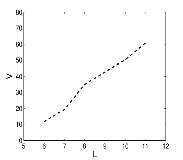
(c)	(d)

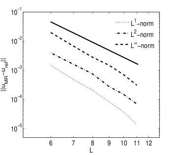
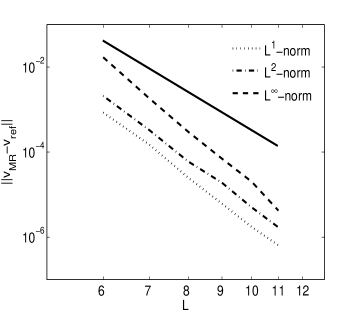
Figure 8. Example 2 (interaction of two flame balls without radiation): (a) speed-up rate $V$, (b) data compression rate $\eta$, for different levels, at time $t=4.0$; (c) errors $\|\bar{u}_{\mathrm{MR}}-\bar{u}_{\mathrm{ref}}\|_{1}$, $\|\bar{u}_{\mathrm{MR}}-\bar{u}_{\mathrm{ref}}\|_{2}$, $\|\bar{u}_{\mathrm{MR}}-\bar{u}_{\mathrm{ref}}\|_{\infty}$ and (d) $\|\bar{v}_{\mathrm{MR}}-\bar{v}_{\mathrm{ref}}\|_{1}$, $\|\bar{v}_{\mathrm{MR}}-\bar{v}_{\mathrm{ref}}\|_{2}$ and $\|\bar{v}_{\mathrm{MR}}-\bar{v}_{\mathrm{ref}}\|_{\infty}$ respectively for different levels $L$, at time $t=4$.

(a)	(b)
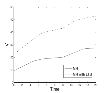
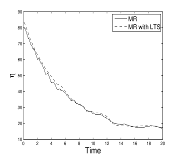
(c)	(d)

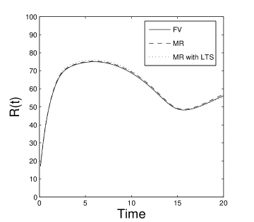
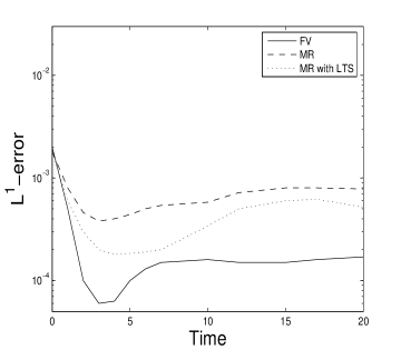
Figure 9. Example 3 (interaction of two flame balls with radiation): Time evolution of speed-up, data compression, and total reaction rates; and $L^{1}$-errors for different methods. $L=10$ multiresolution levels and reference tolerance $\varepsilon_{\mathrm{R}}=7.43\times 10^{-3}$.

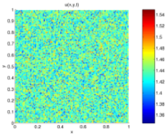
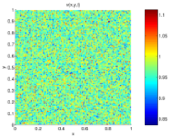
Figure 10. Examples 4 and 5 (Turing pattern-formation): Initial data $u_{0}(x,y)$ (left) and $v_{0}(x,y)$ (right).

8.3. Examples 4 and 5: A Turing model of pattern formation

We select the parameters $a=-0.5$, $b=1.9$, $d=4.8$ and $\gamma=210$. According to the discussion of Section 2.2, these parameters allow diffusion-driven instabilities to evolve. The initial concentration distribution is a normally distributed random perturbation around the stationary state $(u^{0},v^{0})$ for the non-degenerate case, with a variance lower than the amplitude of the final patterns, see Figure 10. For the case of non-degenerate diffusion (Example 4), we use $A(u)$ and $B(u)$ as given by (2.9). For these parameters, the steady state is $(u^{0}=1.4,v^{0}=0.96939)$.

In Example 4 we choose a maximal resolution level of $N_{L}=256^{2}=65536$ control volumes in the finest grid and a reference tolerance given by $\varepsilon_{\mathrm{R}}=2.6\times 10^{-3}$. The time step is the maximum allowed by the CFL condition (3.4). Table 2 summarizes the speed-up rate, compression rate and errors in different norms between the numerical solution by multiresolution and the fine-mesh finite volume reference solution for different times. We depict errors between our multiresolution scheme and a reference FV solution with $N_{L}=1024^{2}=1048576$ control volumes in the finest grid, for different multiresolution levels $L$ in Figure 12 (c) and (d). In this case, the slopes equally indicate a rate of convergence slightly larger than two. Concerning the computation of errors, in Examples 4, 5 and 6 the system is evolved until the “random noise”, which is imposed as an initial condition on the finest grid, has been smoothed sufficiently; then, this solution is projected on coarser levels to obtain auxiliary initial conditions for all the needed levels.

Time	$V$	$\eta$	Species	$L^{1}-$error	$L^{2}-$error	$L^{\infty}-$error
$t=0.05$	7.16	11.3783	$u$	$6.81\times 10^{-4}$	$4.76\times 10^{-5}$	$3.46\times 10^{-3}$
			$v$	$4.09\times 10^{-4}$	$3.92\times 10^{-4}$	$5.38\times 10^{-4}$
$t=0.25$	9.29	11.9756	$u$	$8.37\times 10^{-4}$	$6.94\times 10^{-5}$	$9.93\times 10^{-3}$
			$v$	$4.22\times 10^{-4}$	$5.43\times 10^{-4}$	$8.48\times 10^{-4}$
$t=1.50$	11.87	14.4739	$u$	$9.26\times 10^{-4}$	$2.71\times 10^{-4}$	$2.44\times 10^{-2}$
			$v$	$4.30\times 10^{-4}$	$9.77\times 10^{-5}$	$8.39\times 10^{-3}$

Table 2. Example 4 (Model 2 with non-degenerate diffusion): Corresponding simulated time, CPU ratio $V$, compression rate $\eta$ and componentwise errors.

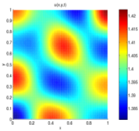
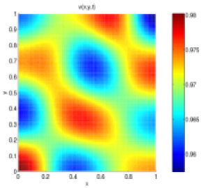
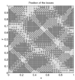
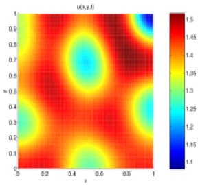
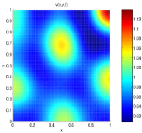
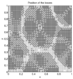
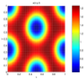
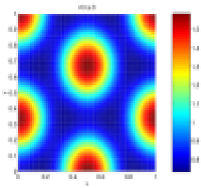
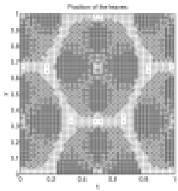
Figure 11. Example 4 (Model 2 with non-degenerate diffusion): Numerical solution for species $u$ (left) and $v$ (right), and leaves of the corresponding tree data structure at times $t=0.05$ (top), $t=0.25$ (middle) and $t=1.5$ (bottom).

(a)	(b)
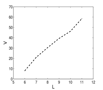
(c)	(d)

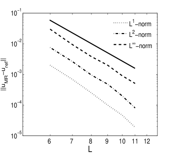
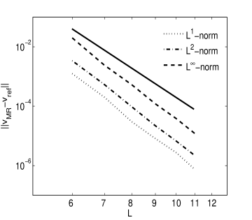
Figure 12. Example 4 (Model 2 with non-degenerate diffusion): (a) CPU acceleration $V$, (b) data compression rate $\eta$, for different levels, at time $t=0.75\,\mathrm{s}$; (c) errors $\|\bar{u}_{\mathrm{MR}}-\bar{u}_{\mathrm{ref}}\|_{1}$, $\|\bar{u}_{\mathrm{MR}}-\bar{u}_{\mathrm{ref}}\|_{2}$, $\|\bar{u}_{\mathrm{MR}}-\bar{u}_{\mathrm{ref}}\|_{\infty}$ and (d) $\|\bar{v}_{\mathrm{MR}}-\bar{v}_{\mathrm{ref}}\|_{1}$, $\|\bar{v}_{\mathrm{MR}}-\bar{v}_{\mathrm{ref}}\|_{2}$ and $\|\bar{v}_{\mathrm{MR}}-\bar{v}_{\mathrm{ref}}\|_{\infty}$ respectively for different levels $L$, at time $t=0.75$.

For Example 5, we use the degenerate diffusion coefficients (2.11) with $u_{\mathrm{c}}=1.2$ and $v_{\mathrm{c}}=0.7$, and employ again the kinetics (2.8), but this time we choose the parameters $a=-0.5$, $b=1.9$, $d=4.8$ and $\gamma=395$. We select a maximal resolution level of $N_{L}=256^{2}=65536$ control volumes in the finest grid, with a reference tolerance given by $\varepsilon_{\mathrm{R}}=3.59\times 10^{-4}$. From Table 3 we see that the multiresolution algorithm allows significant acceleration and data compression rate are significantly increased by the multiresolution algorithm with very good accuracy. Figure 13 indicates that due to the degeneracy of the diffusion given by (2.11), and in contrast to Example 4, species $u$ exhibits patterns with steeper gradients, and especially at $t=0.25$ and $t=1.5$, singularities appear.

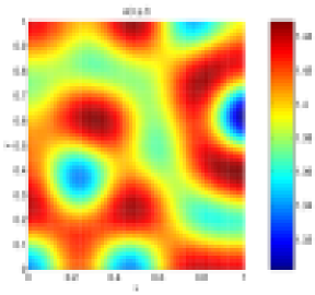
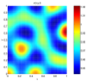
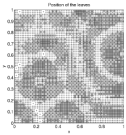
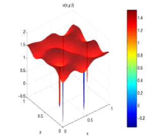
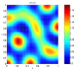
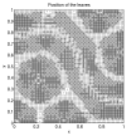
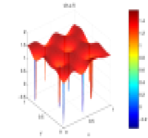
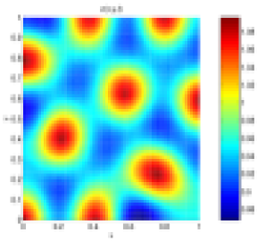
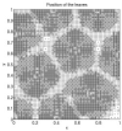
Figure 13. Example 5 (Model 2 with degenerate diffusion): Numerical solution for species $u$ (left) and $v$ (middle), and leaves of the corresponding tree data structure (right) at times $t=0.1$ (top), $t=0.25$ (middle) and $t=1.5$ (bottom).

Time	$V$	$\eta$	Species	$L^{1}-$error	$L^{2}-$error	$L^{\infty}-$error
$t=0.10$	6.32	12.5438	$u$	$6.31\times 10^{-4}$	$5.82\times 10^{-4}$	$2.72\times 10^{-3}$
			$v$	$4.98\times 10^{-4}$	$5.37\times 10^{-4}$	$9.46\times 10^{-4}$
$t=0.25$	9.79	10.3457	$u$	$6.12\times 10^{-4}$	$2.46\times 10^{-5}$	$3.03\times 10^{-3}$
			$v$	$3.91\times 10^{-4}$	$9.22\times 10^{-4}$	$9.92\times 10^{-4}$
$t=1.50$	11.60	10.1984	$u$	$3.42\times 10^{-4}$	$7.34\times 10^{-4}$	$3.40\times 10^{-3}$
			$v$	$2.63\times 10^{-4}$	$4.98\times 10^{-4}$	$2.81\times 10^{-3}$

Table 3. Example 5 (Model 2 with degenerate diffusion): Corresponding simulated time, speed-up rate $V$, compression rate $\eta$ and componentwise errors.

8.4. Example 6: Chemotaxis-growth system

For Example 6, in (2.12) we consider a square domain $\Omega=[0,16]^{2}$ and fix the parameters $\sigma=0.0625$ and $d=1$. The function $h(u,v)$ is given by (2.15) with $\alpha=1$ and $\beta=32$. The growth function $g(u)$ for the species $u$ is given by (2.14), and the chemotactical sensitivity is given by (2.13). This configuration corresponds to the model of chemotaxis and growth presented in [27], which is further analyzed in [17]. Similarly to [17], the initial datum is $(u_{0},v_{0})=(1+\varepsilon(\mathbf{x}),1/32)$, where $\varepsilon(\mathbf{x})$ is a particular smooth perturbation which goes to zero near $(8,8)$. We simulate the process until the solution reaches inhomogeneous stationary states, and we present three cases corresponding to different values of $\nu$, which is responsible for the complexity of the spatial patterns. For example, for $\nu=7$ Figure 14 (middle) shows labyrinth-shaped patterns and for $\nu=10$ (bottom), single filaments and spots. The corresponding adaptive meshes were generated with $N_{L}=512^{2}=262144$ control volumes in the finest grid, with $\varepsilon_{\mathrm{R}}=8.43\times 10^{-4}$. For all these cases we implement locally varying time stepping, so we will choose the maximum CFL number allowed by (3.6), $\mathsf{CFL}_{0}=1$ for the coarsest level and $\mathsf{CFL}_{l}=2^{l}\mathsf{CFL}_{0}$ for finer levels. From Figure 15 we can observe that if we incorporate the local time stepping strategy, a substantial gain (a factor slightly lower than 2, which is consistent with the results by Lamby, Müller, and Stiriba [24]) is obtained in speed-up rate when comparing with a multiresolution calculation using global time stepping. The errors are computed from a reference solution in a grid with $N_{L}=2048^{2}=4194304$ control volumes. We conclude that the errors are kept of the same slope that the errors obtained with a global time step.

The compression rate $\eta$ for both methods is lower than in the previous examples, which could be explained by the complexity and density of the spatial patterns in this particular example.

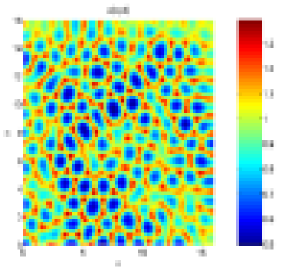
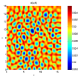
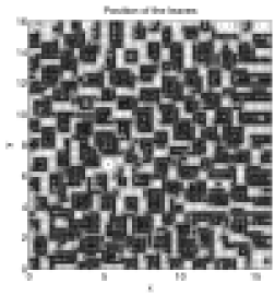
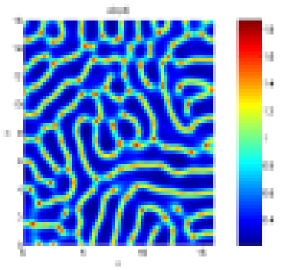
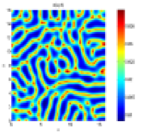
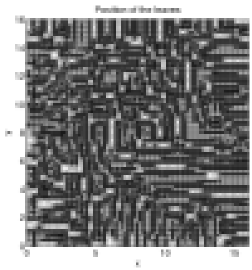
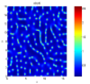
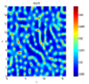
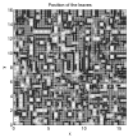
Figure 14. Example 6 (chemotaxis with growth): Numerical solution for species $u$ (left) and $v$ (middle), and leaves of the corresponding tree data structure (right) for $\nu=6.04$ (top), $\nu=7$ (middle) and $\nu=10$ (bottom).

(a)	(b)
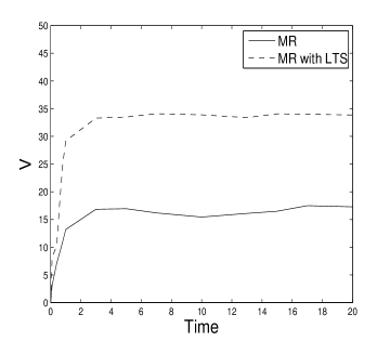
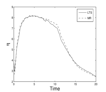
(c)	(d)

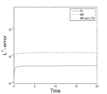
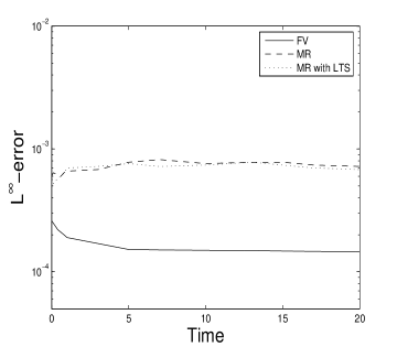
Figure 15. Example 6 (chemotaxis with growth, $\nu=7$): Time evolution for speed-up rate $V$, data compression rate $\eta$ and errors for different methods: Multiresolution scheme with global time step, and multiresolution with locally varying time step.

9. Conclusions

This paper describes an adaptive multiresolution scheme combined with a locally varying time stepping used to approximate solutions of a class of two-dimensional reaction-diffusion systems in Cartesian geometry. Several numerical examples show that the adaptive multiresolution mechanism with a suitable choice of the threshold value represents a gain in CPU time while the errors are kept of the same order as the reference finite volume method. In Examples 3 and 6, we also see that the local time stepping strategy is responsible for a gain in CPU time speed-up for a factor of about 2. Also, the errors between the solution using local time stepping and a reference solution are of the same order that the solution obtained by the adaptive multiresolution with global time stepping.

The motivation to employ explicit schemes only is the following. Even though implicit methods allow larger time steps, we need to iteratively solve a nonlinear system in each time step, using e.g. Newton-Raphson method. The number of iterations is usually controlled by measuring the residual error, and cannot be controlled a priori. Thus, it appears difficult to assess the true benefits of a time-stepping strategy if the basic time discretization is an implicit one.

On the other hand, of course, for the Turing-type pattern formation problem, it is conceded that patterns appear when one eigenvalue goes from negative to positive. At steady state (when the pattern is visible) all the eigenvalues again have negative real part. Thus to converge to steady state once the domain of attraction of the pattern is reached, implicit methods offer significant advantages since they can use larger and larger time steps.

We remark that for hyperbolic problems, the incorporation of an implicit time discretization to the MR-LTS strategy can possibly form a substantial improvement in the speed-up rate, as presented in [31].

References

- [1] M.J. Berger and J. Oliger, Adaptive mesh refinement for hyperbolic partial differential equations, J. Comput. Phys. 53 (1984) 482–512.
- [2] B.L. Bihari and A. Harten, Multiresolution schemes for the numerical solution of 2-D conservation laws I, SIAM J. Sci. Comput. 18 (1997) 315–354.
- [3] P. Biler, Local and global solvability of some parabolic systems modelling chemotaxis, Adv. Math. Sci. Appl. 8 (1998) 715–743.
- [4] N.F. Britton, Reaction-Diffusion Equations and Their Application to Biology, Academic Press, NY, 1986.
- [5] R. Bürger and A. Kozakevicius, Adaptive multiresolution WENO schemes for multi-species kinematic flow models, J. Comput. Phys. 224 (2007) 1190–1222.
- [6] R. Bürger, A. Kozakevicius, and M. Sepúlveda, Multiresolution schemes for degenerate parabolic equations in one space dimension, Numer. Meth. Partial Diff. Eqns. 23 (2007) 706–730.
- [7] R. Bürger, R. Ruiz, K. Schneider, and M. Sepúlveda, Fully adaptive multiresolution schemes for strongly degenerate parabolic equations with discontinuous flux, J. Engrg. Math. 60 (2008) 365–385.
- [8] R. Bürger, R. Ruiz, K. Schneider, and M. Sepúlveda, Fully adaptive multiresolution schemes for strongly degenerate parabolic equations in one space dimension, M2AN Math. Model. Numer. Anal. 42 (2008) 535–563.
- [9] A. Chertok and A. Kurganov, A positivity preserving central-upwind scheme for chemotaxis and haptotaxis models. Preprint (2007); available at http://www.math.tulane.edu/~kurganov/pub.html.
- [10] G. Chiavassa and R. Donat, Point value multiresolution for 2D compressible flows, SIAM J. Sci. Comput. 23 (2001) 805–823.
- [11] G. Chiavassa, R. Donat, and S. Müller, Multiresolution-based adaptive schemes for hyperbolic conservation laws, in Adaptive Mesh Refinement–Theory and Applications, T. Plewa, T. Linde and V.G. Weiss, eds., Springer-Verlag, Berlin, 2003, pp. 137–159.
- [12] C. Chiu and J.L. Yu, An optimal adaptive time-stepping scheme for solving reaction-diffusion-chemotaxis systems, Math. Bio. and Eng. 4 (2007) 187–203.
- [13] A. Cohen, S. Kaber, S. Müller, and M. Postel, Fully adaptive multiresolution finite volume schemes for conservation laws, Math. Comp. 72 (2002) 183–225.
- [14] W. Dahmen, B. Gottschlich-Müller, and S. Müller, Multiresolution schemes for conservation laws, Numer. Math. 88 (2001) 399–443.
- [15] M. Domingues, O. Roussel, and K. Schneider, On space-time adaptive schemes for the numerical solution of partial differential equations, ESAIM: Proc. 16 (2007) 181–194.
- [16] M. Domingues, S. Gomes, O. Roussel, and K. Schneider, An adaptive multiresolution scheme with local time-stepping for evolutionary PDEs, J. Comp. Phys. 227 (2008) 3758–3780.
- [17] M. Efendiev, M. Kläre, and R. Lasser, Dimension estimate of the exponential attractor for the chemotaxis-growth system, Math. Meth. Appl. Sci. 30 (2007) 579–594.
- [18] E. Fehlberg, Low order classical Runge-Kutta formulas with step size control and their application to some heat transfer problems, Computing 6 (1970) 61–71.
- [19] A. Harten, Multiresolution algorithms for the numerical solution of hyperbolic conservation laws, Comm. Pure Appl. Math. 48 (1995) 1305–1342.
- [20] H. Holden, K.H. Karlsen, and N.H. Risebro, On uniqueness and existence of entropy solutions of weakly coupled systems of nonlinear degenerate parabolic equations, Electron. J. Diff. Eqs. 46 (2003) 1–31.
- [21] D. Horstmann, From 1970 until present: the Keller-Segel model in chemotaxis and its consequences, II, Jahresber. Deutsch. Math.-Verein. 106 (2004) 51–69.
- [22] E.F. Keller and L.A. Segel, Model for chemotaxis, J. Theor. Biol. 30 (1971) 225–234.
- [23] S.N. Kružkov, First order quasi-linear equations in several independent variables, Math. USSR Sbornik, 10 (1970) 217–243.
- [24] P. Lamby, S. Müller, and Y. Stiriba, Solution of shallow water equations using fully adaptive multiscale schemes, Int. J. Numer. Meth. Fluids 49 (2005) 417–437.
- [25] T. Leppänen, M. Karttunen, R.A. Barrio, and K. Kaski, The effect of noise on Turing patterns, Progr. Theor. Phys. 150 (2003) (Suppl.) 367–370.
- [26] C. Mascia, A. Porretta, and A. Terracina, Nonhomogeneous Dirichlet problems for degenerate parabolic-hyperbolic equations, Arch. Ration. Mech. Anal. 163 (2002) 87–124.
- [27] M. Mimura and T. Tsujikawa, Aggregating pattern dynamics in a chemotaxis model including growth, Physica A 230 (1996) 499–543.
- [28] P.K. Moore, An adaptive finite element method for parabolic differential systems: some algorithmic considerations in solving in three space dimensions, SIAM J. Sci. Comput. 21(4) (2000) 1567–1586.
- [29] P.K. Moore, Solving regularly and sigularly perturbed reaction–diffusion equations in three space dimensions, J. Comp. Phys. 224 (2007) 601–615.
- [30] S. Müller, Adaptive Multiscale Schemes for Conservation Laws, Springer-Verlag, Berlin, 2003.
- [31] S. Müller and Y. Stiriba, Fully adaptive multiscale schemes for conservation laws employing locally varying time stepping, J. Sci. Comput. 30 (2007) 493–531.
- [32] J.D. Murray, Parameter space for Turing instability in reaction diffusion mechanisms: a comparison of models, J. Theor. Biol. 98 (1982) 143–163.
- [33] J.D. Murray, Mathematical Biology II: Spatial Models and Biomedical Applications, Third Edition, Springer-Verlag, New York, 2003.
- [34] S. Osher and R. Sanders, Numerical approximations to nonlinear conservation laws with locally varying time and space grids, Math. Comp. 41 (1983) 321–336.
- [35] O. Roussel, K. Schneider, A. Tsigulin, and H. Bockhorn, A conservative fully adaptive multiresolution algorithm for parabolic PDEs, J. Comput. Phys. 188 (2003) 493–523.
- [36] O. Roussel and K. Schneider, An adaptive multiresolution method for combustion problems: application to flame ball-vortex interaction, Computers & Fluids 34 (2005) 817–831.
- [37] O. Roussel and K. Schneider, Numerical study of thermodiffusive flame structures interacting with adiabatic walls using an adaptive multiresolution scheme, Combust. Theory Modelling 10 (2006) 273–288.
- [38] J. Schnakenberg, Simple chemical reaction systems with limit cycle behaviour, J. Theor. Biol. 81 (1979) 389–400.
- [39] B. Sjögreen, Numerical experiments with the multiresolution scheme for the compressible Euler equations, J. Comput. Phys. 117 (1995) 251–261.
- [40] A.M. Turing, The chemical basis of morphogenesis, Phil. Trans. Royal Soc. London Ser. B 237 (1952) 37–72.
- [41] T.P. Witelski, Segregation and mixing in degenerate diffusion in population dynamics, J. Math. Biol. 35 (1997) 695–712.