The cluster glass state in the two-dimensional extended t-J model

Abstract

The recent observation of an electronic cluster glass state composed of random domains with unidirectional modulation of charge density and/or spin density on $Bi_{2}Sr_{2}CaCu_{2}O_{8+\delta}$ reinvigorates the debate of existence of competing interactions and their importance in high temperature superconductivity. By using a variational approach, here we show that the presence of the cluster glass state is actually an inherent nature of the model based on the antiferromagnetic interaction ($J$) only, i.e. the well known $t-J$ model. There is no need yet to introduce a competing interaction to understand the existence of the cluster glass state. The long-range pairing correlation is not much influenced by the disorder in the glass state which also has nodes and linear density of states. In the antinodal region, the spectral weight is almost completely suppressed. The modulation also produces subgap structures inside the ”coherent” peaks of the local density of states.

I Introduction

Since the discovery of high temperature superconductors (HTS) two decades ago, many anomalous properties have been reported. One of the most interesting properties is the possible existence of the stripe state consisting of one dimensional charge-density modulation coupled with spin ordering ZaanenPRB89 ; PoilblancPRB89 ; KivelsonRMP03 . The first direct experimental evidence TranquadaNat95 of this stripe state as the ground state is for the non-superconducting $La_{1.48}Nd_{0.4}Sr_{0.12}CuO_{4}$ with the hole density about $1/8$ per unit cell. Since then more evidences of the presence of these have been reported in other cuprate samples MookPRL02 ; FujitaPRL02 . However it seems that the stripe is much more prominent in the LaSrCuO (LSCO) family near $1/8$ doping LakeNature02 ; LucarelliPRL03 and in particular for $La_{1.875}Ba_{0.125}CuO_{4}$ ($LBCO-1/8$) FujitaPRL02 where the charge density or spin density modulation could be considered as an long-ranged order parameter of a phase with broken symmetries. Very recently the high resolution scanning tunneling microscopy (STM) has observed unidirectional domains with periodic density of states modulation in two families of $Ca_{2-x}Na_{x}CuO_{2}Cl_{2}$ and $Bi_{2}Sr_{2}CaCu_{2}O_{8+\delta}$ (BSCCO) KohsakaSci07 ; HowardPRB2003 . These bond-centered electronic patterns with a width of four lattice constants form the so called electronic cluster glass state with short-ranged modulations. Although the modulation is weak, it is still surprising to have the rather high superconducting (SC) transition temperature in this glass state. STM spectra also provided the new puzzling result that there are two different types of spectral gaps in those systems. One is a larger gap with a broader distribution and it seems to be related to the pseudogap. Inside this gap, there is a smaller gap or the so called sub-gap kink with clear $d$-wave like spectra BoyerNP07 ; AlldredgeCM08 . These results and the most recent conflicting results reported by angle-resolved-photo-emission spectra (ARPES) WSLeeNature07 ; KanigelPRL07 raise the question whether there are two energy scales related with two different underlying mechanisms separately responsible for the larger pseudogap and the lower-temperature SC transition. But one feature that most experimental results agree is the presence of the linear density of state (DOS) near the nodal point. It is interesting to note that this has also been reported in the non-superconducting stripe state of $LBCO-1/8$ VallaSci06 .

The observations of these strongly-modulated inhomogeneous states like $LBCO-1/8$ with almost zero SC transition temperature ($T_{c}$) or weakly inhomogeneous cluster glass states in BSCCO with quite high $T_{c}$ have fueled the idea about the presence of competing interactions and underdoped HTS is near the boundary of two distinct phases with different order parameters. The fluctuations KivelsonRMP03 of the order parameters in these adjacent phases could be the mechanism of high temperature superconductivity. Thus it seems like a $d\acute{e}j\grave{a}$ $vu$ that after two decades we are still faced with a daunting question about the appropriate fundamental interactions to model and to understand the HTS. Many people are still not convinced by all those successes AndersonScience87 ; AndersonJPCM04 ; PALeeRMP06 claimed by studying the strong coupling Hubbard model or its equivalent $t-J$ model. In this model the nearest-neighbor antiferromagnetic (AF) spin coupling $J$ is the only relevant interaction besides the usual kinetic energy of electrons (represented by the $t$ term). There are no other competing interactions and certainly no phase boundaries between overdoped and underdoped regimes with different order parameters to be worried.

In this paper we will show that interactions represented by $t$ and $J$ are actually competing with each other. This competition, greatly enhanced by the strong correlation between electrons, has many spatially heterogeneous states almost exactly the same energy as the uniform ground state. The ground state could easily tolerate local spatial modulation of charge density, spin density and even pairing amplitude without much an effect on its SC order parameter. The presence of these very low-energy cluster glass states with a random pattern of short-ranged modulation is an inherent nature of the $t-J$ model. The selection of a particular local electronic pattern as observed in scanning tunneling spectroscopy (STS) for HTS is most likely determined by the effects of impurities, defects and electron-lattice interaction, etc. Random distribution of impurities and defects will not produce long-ranged modulation in the sense of charge-density-wave order or spin-density-wave order unless these is a very strong lattice distortion as demonstrated FujitaPRL02 by the structural transition observed in $LBCO-1/8$. Hence our result for the extended $t-J$ model shows that for weakly inhomogeneous cuprates like BSCCO there is no need to introduce other strong competing interactions with new broken symmetry phases and long-ranged order parameters to produce the observed glass states. The extended $t-J$ model is adequate to explain many of the experimental observations. Depending on the particular type of modulations, the local DOS could either have a node with linear DOS or without a node. These local modulations also produce the sub-gap structures. In addition, these cluster glass states have almost completely suppressed the quasi-particle spectral weight near the antinodal region as observed by ARPES for BSCCO compounds TanakaSci06 .

Before we start with the discussion about the cluster glass states, we should point out that the competition between the kinetic energy represented by $t$ and the magnetic energy represented by $J$ is not a new idea. It is the main reason for the uniform-state phase diagram obtained by the theory of the resonating-valence-bond (RVB) state AndersonScience87 ; AndersonJPCM04 ; PALeeRMP06 . The $J$ term prefers the formation of spin pairing, the so called RVB singlet, or the long-ranged antiferromagnetism. Because of the strong correlation a spin can only hop by exchanging position with a hole, hence the kinetic energy is proportional to the density of holes. But the more hole the system has, the less number of spin there is. Consequently the pairing is also reduced. Thus the pairing amplitude reduces when hole doping increases. Magnetic energy is reduced while kinetic-energy gain increases. It is shown below this competition also happens in individual unit cell.

On the theoretical side the stripe state also has a long history. It was first founded almost two decades ago in the mean-field treatment of the Hubbard model ZaanenPRB89 ; PoilblancPRB89 although the validity of the method in treating strong Hubbard interaction is questionable. Then the extended $t-J$ models were studied by several numerical methods such as the exact diagonalization method HellbergPRL99 , the density matrix renormalization group method WhitePRB98 ; TohyamaPRB1999 and the variational Monte Carlo (VMC) method TohyamaPRB1999 ; KobayashiJLTP1999 . But the results are inconsistent. There are indications that stripe is unstable when the second neighbor hopping, $t^{\prime}$, is included in the $t-J$ model. However, a later VMC study of the $t-t^{\prime}-J$ model HimedaPRL02 indicates that the stripe has about $1\%$ lower energy than the uniform RVB based $d$-wave SC state for most of the negative values of $t^{\prime}$ except when $-t^{\prime}/t$ is less than $0.1$. Similar results were also reported for the Hubbard model MiyazakiJPCS02 . These results pose a new direct contradiction with the experimental findings. Many experimental and theoretical studies have found that $-t^{\prime}/t$ is smallest for LSCO family PavariniPRL01 ; ShihPRL04 ; Hashimoto2008 , thus the stripe state should not be favorable. Yet as mentioned above, among all the cuprates LSCO family has the most solid evidences for the existence of stripe. There are also other problems with the proposed stripe states, such as suppressed pairing correlation and absence of the V-shape DOS at low energy, and we will discuss them below. All of the previous works concentrated on studying periodic stripes with a long-ranged order, it is unclear if the result will hold for the cluster glass state. There are also different kinds of stripes to be considered. It is possible to have only charge density modulation, or only spin density modulation, or only pairing amplitude modulation or with the linear combination of any two or all three of them MillisPRB07 ; Baruch08012436 . Furthermore the relation between these modulations could be correlated or anti-correlated. All these issues are addressed below and their results are compared with the experiments.

II The stripe-like states by the variational Monte Carlo method

We consider the extended $t-J$ Hamiltonian,

$$H=-\sum_{i,j,\sigma}t_{ij}\left(\tilde{c}_{i\sigma}^{{\dagger}}\tilde{c}_{j\sigma}+h.c.\right)+J\sum_{<i,j>}\mathbf{S}_{i}\cdot\mathbf{S}_{j}$$ (1)

which has been used to describe many physical systems in the high-temperature superconductors KYYangPRB06 . The hopping amplitude $t_{ij}=t$, $t^{\prime}$, and $t^{\prime\prime}$ for sites $i$ and $j$ being the nearest-, the second-nearest, and the third-nearest-neighbors, respectively. We restrict the electron creation operators $\tilde{c}_{i\sigma}^{{\dagger}}$ to the subspace with no-doubly-occupied sites. $\mathbf{S}_{i}$ is the spin operator at site $i$ and $<i,j>$ means that the interaction occurs only for the nearest-neighboring sites. In the following, we mainly focus on the case $t^{\prime\prime}=-t^{\prime}/2$ and $J/t=0.3$ at hole doping $1/8$.

We shall follow the work by Himeda et al. HimedaPRL02 to construct the variational wave functions. In the mean-field theory we assume a local AF order parameter, the staggered magnetization $m_{i}$, and nearest neighbor pairing order parameter $\Delta_{ij}$. Thus the effective mean-field Hamiltonian is reduced to

$$H_{MF}=\sum_{i,j}\left(\begin{array}[]{cc}c^{{\dagger}}_{i\uparrow}&c_{i\downarrow}\\ \end{array}\right)\left(\begin{array}[]{cc}H_{ij\uparrow}&D_{ij}\\ D^{\ast}_{ji}&-H_{ji\downarrow}\\ \end{array}\right)\left(\begin{array}[]{c}c_{j\uparrow}\\ c^{{\dagger}}_{j\downarrow}\\ \end{array}\right),$$ (2)

where the matrix elements

$$H_{ij\sigma}= - \left(t_{v}\sum_{\beta=N}+t^{\prime}_{v}\sum_{\beta=NN}+t^{\prime\prime}_{v}\sum_{\beta=NNN}\right)\delta_{j,i+\beta}$$ (3)

$$+ \left(\rho_{i}-\mu_{v}+\sigma(-1)^{x_{i}+y_{i}}m_{i}\right)\delta_{j,i},$$

$$D_{ij}=\sum_{\beta=N}\Delta_{ij}\delta_{j,i+\beta}.$$ (4)

Here $\beta=N$, $NN$, and $NNN$ correspond to the nearest-, the next-nearest, and the third-nearest-neighbors, respectively, and $\sigma=\uparrow$(1) or $\downarrow$(-1). The local charge density is controlled by $\rho_{i}$ and $\mu_{v}$ is the variational parameter for the chemical potential. For periodic stripes we assume charge density $\rho_{i}$ and staggered magnetization $m_{i}$ are anti-correlated, ${\it i.e.}$ there are more holes at sites with minimum staggered magnetization. For simplicity, we assume these spatially varying functions with simple forms:

$$\rho_{i}=\rho_{v}\cos[4\pi\delta\cdot(y_{i}-y_{0})],$$ (5)

$$m_{i}=m_{v}\sin[2\pi\delta\cdot(y_{i}-y_{0})],$$ (6)

where $\delta$ is the doping density and is $1/8$ in this paper. We have also taken the lattice constant to be our unit. Here we assume the stripe extends uniformly along the $x$ direction. $y_{0}=0$ $(1/2)$ corresponds to the site- (bond-) centered stripe. In this paper, we will only focus on the bond-centered stripe since the variational energy difference between the site- and bond-centered stripes is very small (not shown) within the finite cluster RaczkowskiPRB07 ; CapelloPRB08 .

Besides staggered magnetization and charge density, the nearest neighbor pairing $\Delta_{ij}$ can also have a spatial modulation. There are several different stripes we can choose. If $\Delta_{ij}$ has the same period $1/\delta$ as the staggered magnetization but it is $\pi$ phase shifted, this is the so called ”antiphase” stripe studied by a number of groups HimedaPRL02 ; RaczkowskiPRB07 ; CapelloPRB08 ; HimedaJPCS02 . In this stripe state, the bond-average $\Delta_{ij}$ is zero and there is no net pairing. Hole density is maximum at the sites with maximum pairing amplitude $|\Delta_{ij}|$ and minimum staggered magnetization $|m_{i}|$.

Another more general choice is to have the spatial variation of $\Delta_{ij}$ of the form,

$$\Delta_{i,i+\hat{x}} = \Delta^{M}_{v}\cos[4\pi\delta\cdot(y_{i}-y_{0})]-\Delta^{C}_{v},$$

$$\Delta_{i,i+\hat{y}} = -\Delta^{M}_{v}\cos[4\pi\delta\cdot(y_{i}-y_{0})+2\pi\delta]+\Delta^{C}_{v}.$$ (7)

The bond-average $\Delta_{ij}$ is determined by the constant $\Delta^{C}_{v}$. If both $\Delta^{M}_{v}$ and $\Delta^{C}_{v}$ are positive, then the hole density is maximum at sites with smallest pairing amplitude $|\Delta_{ij}|$ and smallest magnetization $|m_{i}|$. This is similar to the phase diagram ShihLTP05 ; ChouJMMM07 predicted by the uniform RVB and AF states, when hole density is small both staggered magnetization and pairing amplitude are larger. Thus we will denote this state as the AF-RVB stripe. For AF-RVB stripe the period of $\Delta_{ij}$ is the same as the charge-density modulation $\rho_{i}$. This period, $1/2\delta$, is only half of the period for the antiphase or $\pi$ phase stripe. Besides the antiphase stripe and AF-RVB stripes, we could also have the AF stripe without both $\Delta^{M}_{v}$ and $\Delta^{C}_{v}$ or the charge-density stripe without any staggered magnetization but with pairing amplitude modulation.

In general we have total seven variational parameters $\mu_{v}$, $t^{\prime}_{v}$, $t^{\prime\prime}_{v}$, $\rho_{v}$, $m_{v}$, $\Delta^{M}_{v}$, and $\Delta^{C}_{v}$ with $t_{v}$ set to be 1. Once these parameters are given, we diagonalize the mean-field Hamiltonian in equation (2). By solving the Bogoliubov de Gennes (BdG) equations

$$\sum_{j}\left(\begin{array}[]{cc}H_{ij\uparrow}&D_{ij}\\ D^{\ast}_{ji}&-H_{ji\downarrow}\\ \end{array}\right)\left(\begin{array}[]{c}u^{n}_{j}\\ v^{n}_{j}\\ \end{array}\right)=E_{n}\left(\begin{array}[]{c}u^{n}_{i}\\ v^{n}_{i}\\ \end{array}\right),$$ (8)

and then obtain $N$ positive eigenvalues $E_{n}$ ($n=1-N$) and $N$ negative eigenvalues $\bar{E}_{n}$ with corresponding eigenvectors $(u^{n}_{i},v^{n}_{i})$ and $(\bar{u}^{n}_{i},\bar{v}^{n}_{i})$. The eigenvectors are used to construct the mean-field wave function HimedaPRL02 $|\psi\rangle$ by using Bogoliubov transformation

$$\left(\begin{array}[]{c}\gamma_{n}\\ \bar{\gamma}_{n}\\ \end{array}\right)=\left(\begin{array}[]{cc}u^{n}_{i}&v^{n}_{i}\\ \bar{u}^{n}_{i}&\bar{v}^{n}_{i}\\ \end{array}\right)\left(\begin{array}[]{c}c_{i\uparrow}\\ c^{{\dagger}}_{i\downarrow}\\ \end{array}\right).$$ (9)

The trial wave function $P|\psi\rangle$ with a Gutzwiller projector $P$ can be constructed by creating all negative energy states and annihilating all positive energy states on a vacuum of electrons $|0\rangle$. Then we formulate the wave function in the Hilbert space with the fixed number of electrons $N_{e}$,

$$|\Phi\rangle=PP_{N_{e}}|\psi\rangle = PP_{N_{e}}\prod_{n}\gamma_{n}\bar{\gamma}^{{\dagger}}_{n}|0\rangle$$

$$\propto P\left(\sum_{i,j}(\hat{U}^{-1}\hat{V})_{ij}c^{{\dagger}}_{i\uparrow}c^{{\dagger}}_{j\downarrow}\right)^{N_{e}/2}|0\rangle,$$

where $\hat{U}_{ij}=u^{i}_{j}$ and $\hat{V}_{ij}=v^{i}_{j}$. We optimize the variational energy $E=\langle\Phi|H|\Phi\rangle/\langle\Phi|\Phi\rangle$ by using the stochastic reconfiguration algorithm SorellaPRB01 . Additionally, to reduce the boundary-condition effect in numerical studies PoilblancPRB91 , we average the energies over the four different boundary conditions which is periodic or antiperiodic in either $x$ or $y$ direction.

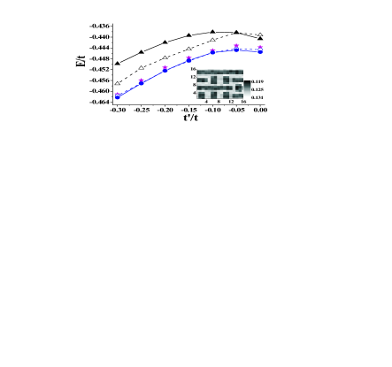
Figure 1: Variational energies of the bond-centered AF-RVB stripe state and uniform $d$-wave RVB state as function of $t^{\prime}/t$. The data have been optimized for $1/8$ doping on the $16\times 16$ lattice system. The filled (empty) symbols represent the energies of uniform $d$-wave RVB state (AF-RVB stripe state). The triangles (circles) indicate the wave functions without (with) the hole-hole correlation of equation (11). The asterisks correspond to the random stripe states with the Jastrow factor of equation (11). Inset: The hole density of the random stripe state optimized in the case of $(t^{\prime},t^{\prime\prime},J)/t=(-0.3,0.15,0.3)$.

Fig.1 shows the $t^{\prime}/t$ dependence of the variational energies for the hole density $\delta=1/8$. Firstly, we have shown that the AF-RVB stripe state (the empty triangles) becomes more stable than uniform $d$-wave RVB state (the filled triangles) as decreasing $t^{\prime}/t$ further from $-0.05$. It is worth noting that the AF-RVB stripe state for $t^{\prime}/t<-0.05$ has the vanishing pairing parameters $\Delta^{C}_{v}$ and $\Delta^{M}_{v}$ but large $m_{v}$ and finite $\rho_{v}$. Therefore, we can consider this stripe state without SC order as the antiphase AF stripe state ZaanenPRB89 . The hole density and the staggered magnetization are plotted as a function of positions for a typical AF stripe (filled circles) in Fig.2(a) and (b), respectively. The AF stripe pattern with a very large hole-density variation is essentially a nano-scale phase separation with hole-rich and hole-poor regions alternating. This is consistent with what has been obtained by Himeda et al. HimedaPRL02 although they did not include $t^{\prime\prime}$ which is set to be $-t^{\prime}/2$ here.

In our previous calculations to study the possibility of phase separation in the $t-J$ model ShihJPCS2001 , we found the tendency to overestimate the strength of the pairing of holes. If we reduce this strength by going beyond the simple trial wave functions used in our discussion above we could push the phase separation boundary to a much higher value of $J/t$. A simpler way to make this adjustment is to introduce the hole-hole repulsion Jastrow factorHellbergPRL91 ; ValentiPRL92 ; SorellaPRL02 :

$$P_{J}=\prod_{i<j}\left(1-(1-r^{\alpha}_{ij}\cdot v^{\delta_{j,i+\beta}}_{\beta})\cdot n^{h}_{i}n^{h}_{j}\right)$$ (11)

with

$$r_{ij}=\sqrt{\sin^{2}\left(\frac{\pi}{L_{x}}(x_{i}-x_{j})\right)+\sin^{2}\left(\frac{\pi}{L_{y}}(y_{i}-y_{j})\right)},$$

where $n^{h}_{i}=1-\Sigma_{\sigma}c^{{\dagger}}_{i\sigma}c_{i\sigma}$. The three parameters $v_{\beta}$ of $\beta=N$, $NN$, and $NNN$ are for short-ranged hole-hole repulsion (attraction) if these values are less (greater) than 1. The factor $r^{\alpha}_{ij}$ is for long-ranged correlations HellbergPRL91 and it is repulsive if $\alpha$ is positive. $L_{x}$ and $L_{y}$ are the number of sites in the $x$ and $y$ direction, respectively. We have found that the variational energy of the periodic stripe state without including the Jastrow factors is very sensitive to boundary conditions. However the Jastrow factor is capable of reducing the dependence of the boundary conditions.

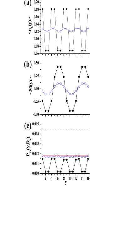
Figure 2: The profiles of (a) hole density, (b) staggered magnetization and (c) pair-pair correlation function with $R_{y}=8$ for the optimized states at $1/8$ doping in the extended $t-J-$ model with $t^{\prime}/t=-0.3$ and $J/t=0.3$. The filled (empty) circles correspond to the AF-RVB stripe state without (with) hole-hole repulsion. In (c), the dashed (dashed-dotted) line indicates the uniform $d$-wave RVB state without (with) hole-hole repulsion. The red solid line corresponds to the random stripe state with hole-hole repulsive Jastrow correlation. All quantities are calculated on a $16\times 16$ lattice system with the periodic and antiperiodic boundary conditions along the x and y directions, respectively.

As shown in Fig.1, when the hole-hole repulsion of equation (11) is included in our VMC calculation, both the uniform $d$-wave RVB state (filled circles) and the AF-RVB stripe state (empty circles) have gained significant energies. In particular, the uniform $d$-wave RVB state has gained about $2\sim 3\%$ in total energy. It indicates that for the extended $t-J$ model the holes are not bounded as tightly as estimated by the simple RVB trial wave functions. It also implies that the nano-scale phase separation of the AF stripe will not be preferable. Indeed, the lowest energy stripe state does not favor the AF stripe but the AF-RVB stripe with a much more reduced staggered magnetization as shown in Fig.2(b) and a larger pairing parameter $\Delta^{C}_{v}$. Now the hole density has a much smaller variation as shown by the empty circles in Fig.2(a).

It is surprising to find out that for all $t^{\prime}/t$, the AF-RVB stripe state is almost degenerate in variational energy with the uniform $d$-wave RVB state. This is quite remarkable as the two trial wave functions are very different. As an illustration we show in Fig.2(a) and (b) the variation of the hole density and the staggered magnetization along the modulation direction, respectively, for an AF-RVB stripe state (empty circles). It should be noticed that not only the hole density is completely uniform for $d$-RVB state but there is also no staggered magnetization at all. Instead of periodic stripes, we have also examined the stripe state with $4\times 4$ patches in the $16\times 16$ lattice system. For each patch, we choose a direction of the stripe, $x$ or $y$, randomly. We consider this state as random stripe state. For simplicity, we still use the same equations (5-7,11). The hole-density modulation of a random stripe state has been shown in the inset of Fig.1. As shown in Fig.1, the random stripe states with the Jastrow factors of equation (11) also have the optimized energies almost identical to uniform $d$-wave RVB and AF-RVB stripe states even though we have not optimized parameters on very bond or site independently. These optimized random stripe states have finite $m_{v}$ and $\Delta^{C}_{v}$ but smaller $\Delta^{M}_{v}$ (less than one third of $\Delta^{C}_{v}$).

We believe this energy degeneracy is caused mainly by two reasons. The first reason is that the terms in the $t-J$ Hamiltonian are all local within nearest neighbors or next nearest neighbors. The second reason is that the hopping terms and spin interaction not only are of the same order of magnitude but they are competing against each other. We have found the energy competition between the kinetic energy and spin interaction is very robust among different states (not shown). Their competition is enhanced by the no-doubly occupancy constraint as the presence of holes will suppress the spin interaction to zero. Thus it is possible to have locally different spin-hole configurations with different emphasis on the kinetic energy or the spin energy. Some of these patterns have lower kinetic energy but higher magnetic energy than the uniform $d$-RVB state and some with opposite energetics.

There are at least two important implications of this energy degeneracy. The first one is that the inhomogeneous states are quite robust in the extended $t-J$ models without the need for introducing any other large interactions. States with different local arrangement of spin and holes may have very similar energies. The second implication is that any small additional interaction could break the degeneracy. If we consider the ”realistic” situation of cuprates with large numbers of impurities, disorders and electron-lattice interactions, the inhomogeneous states could be much more numerous and complex than we have expected. Materials made with different processing conditions could also produce different inhomogeneous states. Since all these are presumably secondary interactions smaller than the dominant $t$ and $J$, the modulations of charge density, staggered magnetization and pairing are expected to be small. If one of the interactions, like electron-lattice interaction, becomes quite strong as observed in $LBCO-1/8$ VallaSci06 , then the modulation will also become larger and longer ranged.

We have also investigated the pair-pair correlation function for the optimized states with/without hole-hole repulsive Jastrow factors in the case of $(t^{\prime},t^{\prime\prime},J)/t=(-0.3,0.15,0.3)$. The singlet pair-pair correlation function along the modulated direction (y direction) is defined as

$$P_{xx}(y,R_{y})=\frac{1}{L_{x}}\sum_{x}\frac{|\langle\Phi|\Delta^{{\dagger}}_{x}(r)\Delta_{x}(r+R_{y})|\Phi\rangle|}{\langle\Phi|\Phi\rangle},$$ (12)

where $r=(x,y)$ and $\Delta^{{\dagger}}_{x}(r)=c^{{\dagger}}_{r\uparrow}c^{{\dagger}}_{r+\hat{x}\downarrow}-c^{{\dagger}}_{r\downarrow}c^{{\dagger}}_{r+\hat{x}\uparrow}$ creates a singlet pair of electrons among the nearest neighbors along $x$ direction for each site $r$. Here, we focus on the long range correlation, and thus set $R_{y}=8$ to be the largest distance on $16\times 16$ lattice system. In Fig.2(c), it is shown that the hole-hole repulsion suppresses the long-range pair-pair correlation about three times in the uniform $d$-wave RVB state. We have also found that without hole-hole repulsive correlation, the long-range pair-pair correlation is much more reduced in the AF-RVB stripe state than uniform $d$-wave RVB state, because the AF-RVB stripe state has almost vanishing $\Delta^{C}_{v}$. Due to large $m_{v}$, this AF-RVB stripe state shows much larger amplitude of the $P_{xx}$ modulation. However, after considering the hole-hole repulsion, the AF-RVB stripe and uniform $d$-wave RVB states have almost the similar magnitude of pair-pair correlation as shown by the empty circles and dashed-dotted line in Fig.2(c), respectively. For the random stripe state shown in the inset of Fig.1 the average value $P_{xx}$ for the whole system is shown as the red solid line in Fig.2(c). It is essentially the same as the value of uniform $d$-wave RVB state and the periodic AF-RVB stripe state. Although the staggered magnetization for the random stripe state has larger variation than the periodic stripe state shown in Fig.2(b), the pairing correlation is unchanged. These results indicate that the long-range pair-pair correlation is mostly determined by the value of $\Delta^{C}_{v}$ and is rather insensitive to the modulation of the hole density and staggered magnetization. Thus we also expect to have a robust $d$-wave node observed by recent experiments KohsakaSci07 ; AlldredgeCM08 . This will be shown below.

III Density of states by the Gutzwiller approximation

According to the VMC calculation for the extended $t-J$ model, it is likely that there are a number of inhomogeneous states close in energy to the uniform ground state. Then, some sort of small perturbation may choose a particular stripe state as the ground state. Assuming such a situation, here we regard a stripe state as the ground state, and consider the projected quasi-particle excitation spectra. However, calculation of the excited states by the VMC method is computationally very expensive, and it takes too much time to investigate wide parameter range to obtain general properties of the stripe states. Furthermore, one can take only a limited system size and it is difficult to obtain dense spectra.

Therefore, as a first step, we use a Gutzwiller mean-field approximation for this purpose. The minimization of the total energy yields a BdG equation Fukushima08012280 . Usually the parameters in the BdG equations are solved self-consistently to find an optimal solution. However, since we already have the assumed inhomogeneous ground state here, we shall use parameter sets obtained from VMC results and diagonalize the BdG Hamiltonian only once, instead of solving self-consistently. Furthermore, for convenience, we slightly modify the Gutzwiller projection by attaching fugacity factors. Namely, we assume that $P_{\lambda}|\psi\rangle$ is the ground state and that $P_{\lambda}\gamma_{n}^{\dagger}|\psi\rangle$ are the excited states, where $P_{\lambda}\equiv P\prod_{i\sigma}\lambda_{i\sigma}^{n_{i\sigma}}$, and $\lambda_{i\sigma}$ is a fugacity factor to impose the local electron density conservation for each spin, namely, $\frac{\langle\psi|P_{\lambda}\hat{n}_{i\sigma}P_{\lambda}|\psi\rangle}{\langle\psi|P_{\lambda}^{2}|\psi\rangle}=\frac{\langle\psi|\hat{n}_{i\sigma}|\psi\rangle}{\langle\psi|\psi\rangle}$ for any $i$ and $\sigma$. The quasi-particle operators $\gamma_{n}^{\dagger}$ are obtained by solving the BdG Hamiltonian. In addition, here we do not take into account the Jastrow factor as it only affects the hole-hole correlation slightly but not the local DOS studied below. Then, under the assumption of the non-self-consistency, the BdG Hamiltonian is represented by equation (2). With this formulation, $P_{\lambda}\gamma_{n}^{\dagger}|\psi\rangle$ of different $n$ are approximately orthogonal to each other Fukushima08012280 , and thus we expect that it is suitable to use $P_{\lambda}$ instead of $P$ for our purpose here. Since the result presented below is qualitatively not very sensitive to small change of the parameters, we expect that such a modification of the projection should not affect the results qualitatively.

Figure 3: Spatially averaged local DOS for the random stripe states calculated by the non-self-consistent BdG equation. (a) For $\Delta_{v}^{C}\neq 0$, we use parameters optimized by the VMC, $t^{\prime}_{v}=-0.35$, $t^{\prime\prime}_{v}=0.16$, $m=0.15$, $\rho=0.03$, $\Delta_{v}^{C}=0.28$ , $\Delta_{v}^{M}=0.02$, but $\mu=-0.875t_{v}$ is adjusted to realize $1/8$ filling, in units of $t_{v}$. (b) The same parameters except for $\Delta_{v}^{C}=0$.

Then, by taking the most dominant terms, the local DOS is represented by

$$N_{\uparrow}(R,\omega)=g^{t}_{R\uparrow}\sum_{n}|u_{R}^{n}|^{2}\delta(\omega-E_{n}),$$ (13)

$$N_{\downarrow}(R,\omega)=g^{t}_{R\downarrow}\sum_{n}|v_{R}^{n}|^{2}\delta(\omega+E_{n}),$$ (14)

where index $n$ runs for both positive and negative eigenvalues. Note that only the position dependent constant $g^{t}_{R\sigma}\equiv{(1-n_{R\uparrow}-n_{R\downarrow})}/{(1-n_{R\sigma})}$ is multiplied in front of the local DOS by the standard BdG formalism. Since the result of the site-centered stripe is very similar to that of the bond-centered stripe, we show only the latter. Here we shall only discuss our results for the random stripe state. For the random stripe state considered above, each randomly oriented domain is assumed to have the same parameters so that the VMC calculation is possible. Ideally we should have optimized these variational parameters on every bond or every site. Then we expect to have a much broader distribution of these parameters. To simulate this effect, we simply replace each $\Delta_{ij}$ by $(1+\xi_{ij})\Delta_{ij}$, where $\xi_{ij}$ is a random variable which has the Gaussian distribution around 0 with the standard deviation of 1. We use a supercell of size 32$\times$32 sites, and the same configuration is repeated as 20$\times$20 supercells to obtain the local DOS. The Fourier transform with respect to the supercell index is similar to a system of small clusters with many twisted boundary conditions.

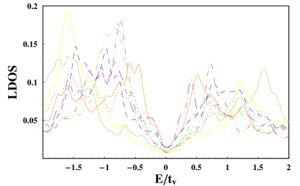
Figure 4: Local DOS at eight different positions for the random stripe states with $\Delta_{v}^{C}\neq 0$ calculated by the non-self-consistent BdG equation.

As shown in Fig.3(a), the spatially averaged $\sum_{\sigma}N_{\sigma}(R,\omega)$ for the AF-RVB stripe ($\Delta_{v}^{C}\neq 0$) has a V-shape at low energy. On the other hand for an antiphase stripe which has $\Delta_{v}^{C}=0$ there is no V-shape as shown in Fig.3(b). The energy level is broadened with a width of $0.05t_{v}$. In Fig.3(b), there is a very small dip at $E=0$, it would be bigger if $\Delta_{v}^{M}$ increases. Our results are consistent with the very recent report by Baruch and Orgad Baruch08012436 . In general, there is no V-shape DOS for the antiphase stripe. For the same system as Fig.3(a), in Fig.4 we plot the position dependence of local DOS at randomly chosen 8 sites. The low energy spectra seem less influenced by the disorder than high energy. This result shows that the node and the low energy V-shape DOS are robust against this kind of inhomogeneity. This is possible because nodal $k$-points do not have many states to mix with and also the suppression of impurity scattering note1 . The sub-gap structures BoyerNP07 ; AlldredgeCM08 also seem to be quite apparent. If we switch off the random variables $\xi_{ij}$, the gap variations from site to site are small. These gap variations grow larger as distributions of $\xi_{ij}$ become wider.

The key to understand the absence of V-shape in the Local DOS for the antiphase stripe is the Fourier transform of the modulated $\Delta_{ij}$ term written as,

$$\Delta_{v}^{M}\sum_{k}\cos k_{x}(e^{-i\theta}c_{k+q,\uparrow}^{\dagger}c_{-k,\downarrow}^{\dagger}+e^{i\theta}c_{k-q,\uparrow}^{\dagger}c_{-k,\downarrow}^{\dagger}+\text{h.c.})\\ -\frac{\Delta_{v}^{M}}{2}\sum_{k}\bigg{[}\left(e^{ik_{y}}+e^{-i(k_{y}+q_{y})}\right)e^{i(\frac{q_{y}}{2}-\theta)}c_{k+q,\uparrow}^{\dagger}c_{-k,\downarrow}^{\dagger}\\ +\left(e^{ik_{y}}+e^{-i(k_{y}-q_{y})}\right)e^{-i(\frac{q_{y}}{2}-\theta)}c_{k-q,\uparrow}^{\dagger}c_{-k,\downarrow}^{\dagger}+\text{h.c.}\bigg{]},$$ (15)

where $\theta=0$ for site-centered stripes and $\theta=q_{y}/2$ for bond-centered stripes; $q=(0,\pi/4)$ for the antiphase stripe, and $q=(0,\pi/2)$ for the AF-RVB stripe. What is important here is that it contains only pairing with nonzero center-of-mass momentum as the FFLO state QWangPRL06 . In the case of zero-momentum pairing as the conventional BCS theory, the spin-up electron band couples with the spin-down hole band (the upside-down down electron band). These bands intersect at the Fermi level, and a gap opens if $\Delta_{k}\neq 0$. In the case of finite-$q$ pairing, however, the spin-up electron band couples with $\pm q$ shifted spin-down hole bands, and thus the band intersections occur not at the Fermi level. Therefore, a gap does not open at the Fermi level. The constant $\Delta^{C}_{v}$ term which forms the usual Cooper pair is necessary for having the node and the V-shape DOS.

To compare with ARPES experiments, $A(k,\omega)$ is also calculated. Since $A(k,\omega)$ is regarded as the local DOS in the $k$-space, Let us take the Fourier transform of renormalized $u_{R}^{n}$, $v_{R}^{n}$, namely,

$$(\tilde{u}_{k}^{n},\tilde{v}_{k}^{n})\equiv\frac{1}{\sqrt{N_{\rm site}}}\sum_{R}e^{-ikR}\left(g^{t}_{R\uparrow}u_{R}^{n},g^{t}_{R\downarrow}v_{R}^{n}\right).$$ (16)

Then, $A_{\sigma}(k,\omega)$ is written as

$$A_{\uparrow}(k,\omega)=\sum_{n}|\tilde{u}_{k}^{n}|^{2}\delta(\omega-E_{n}),$$ (17)

$$A_{\downarrow}(k,\omega)=\sum_{n}|\tilde{v}_{k}^{n}|^{2}\delta(\omega+E_{n}).$$ (18)

Figure 5: $\sum_{\sigma}A_{\sigma}(k,E)$ for the random stripe state with $\Delta_{C}\neq 0$. Dotted lines are for uniform $d$-wave RVB state ($\rho_{v}=0,m_{v}=0,\Delta_{v}^{M}=0$). (a) Nodal and (b) near antinodal region.

Fig.5 shows $\sum_{\sigma}A_{\sigma}(k,\omega)$ of the random stripe state with $\Delta_{v}^{C}\neq 0$, where each of the $\delta$-function spectra are replaced with a Lorentzian distribution with $\delta E=0.05t_{v}$. In comparison with the uniform $d$-wave RVB state, the spectral weight around the antinodal region is much strongly reduced than near the node.

IV Conclusions

In summary, we have used a variational approach to examine the possibility of having inhomogeneous ground states within the extended $t-J$ model with $1/8$ doping. We considered states with spatial modulation of charge density, staggered magnetization and pairing amplitude. Besides the antiphase or inphase stripes considered by many groups we have proposed a new AF-RVB stripe. In this stripe state, we assume there is a constant pairing amplitude besides the various modulation. In addition to considering states with periodic stripes we also consider random stripe states to simulate the cluster glass state observed by experiments KohsakaSci07 . By improving the trial wave functions with the introduction of hole-hole repulsive correlation, we have greatly improved the variational energies by several percents for both uniform RVB $d$-wave SC state and states with periodic AF-RVB stripes for realistic values of $t^{\prime}/t$. Most surprisingly the random stripe state essentially also has the same energy as the uniform state in spite of our oversimplified assumption that all the stripe domain has the same patterns of modulation instead of each site or bond with different values. This random stripe state also has about the same long-range pair-pair correlation as the uniform or periodic stripe state even though there are significant staggered magnetization and charge variation from site to site. Then we also examined the local DOS and the spectral weight of the random stripe state by using Gutzwiller approximation. We found the V-shape DOS and the node are still present at every site. The local DOS measured at different positions shows a broad variation of the gaps and also it has sub-gap structures seen in experiments BoyerNP07 ; AlldredgeCM08 . The spectral weight at the antinodal direction is negligibly small but finite around the node. All these results are quite consistent with experiments reported for cluster glass state in BSCCO KohsakaSci07 .

Our result also resolves an inconsistency with experiments derived from previous theoretical calculations without including the hole-hole repulsion in the trial wave functions. Stripe is neither stabilized nor destabilized by the long range hopping. In fact, due to the competition between the kinetic energy gain and magnetic interaction, it is very natural to have the spatial modulation, in periodic or random configuration, of charge density, magnetization and even pairing amplitude. The constraint of disallowing doubly occupation of electrons at each lattice site has significantly enhanced the competition. Many local arrangements of spin and hole configurations could give almost identical total energy as the uniform solution.

Recently, Capello et al. CapelloPRB08 have also found that the energy of the periodic RVB stripe state is very close to that of the uniform RVB state by using a variational calculation. They have considered several possibilities for the stability of the RVB stripe state, such as lattice distortion, t’-effect, and long-range Coulomb repulsion with the conclusion that uniform RVB state is still the lowest energy state. This is very consistent with our conclusion although we have included the antiferromagnetic order in the stripe state. The issue about whether AF is present in the stripe will be discussed in the future. They have not considered the cluster glass state with random AF-RVB stripe domains which is also a good candidate for the ground state.

The presence of inhomogeneous or cluster glass states is apparently a very natural consequence of the $t-J$ model. There is no need for introducing additional interactions to generate such states. In fact we showed that the RVB state with a finite constant pairing is quite compatible with the local variations of charge density, magnetization and even pairing amplitude. As long as this modulation is not overly strong, the superconductivity still survives as the node and V-shape DOS are still present. In a realistic material, other interactions such as impurity, disorder, and electron-lattice interactions, etc., no doubt will help to determine the most suitable local configuration of spins and holes but they will not produce a globally ordered state unless there is a very strong and dominant interaction like the electron-lattice interaction seen in $La_{2-x}Ba_{x}CuO_{4}$ at $1/8$ doping. The verification of this is left for future work.

V Acknowledgments

This work is supported by the National Science Council in Taiwan with Grant no.95-2112-M-001-061-MY3. The calculations are performed in the IBM Cluster 1350, FormosaII Cluster and IBM P595 in the National Center for High-performance Computing in Taiwan, and the PC Farm and Euler system of Academia Sinica Computing Center in Taiwan.

References

- (1) J. Zaanen and O. Gunnarsson, Phys. Rev. B 40, 7391 (1989).
- (2) D. Poilblanc and T. M. Rice, Phys. Rev. B 39, 9749 (1989).
- (3) S. A. Kivelson et al., Rev. Mod. Phys. 75, 1201 (2003).
- (4) J. M. Tranquada et al., Nature 375, 561 (1995).
- (5) H. A. Mook, P. Dai, and F. Dogan, Phys. Rev. Lett. 88, 097004 (2002).
- (6) M. Fujita, H. Goka, K. Yamada, and M. Matsuda, Phys. Rev. Lett. 88, 167008 (2002).
- (7) Y. S. Lee et al., Phys. Rev. B 60, 3643 (1999).
- (8) B. Lake et al., Nature 415, 299 (2002).
- (9) A. Lucarelli et al., Phys. Rev. Lett. 90, 037002 (2003).
- (10) Y. Kohsaka et al., Science 315, 1380 (2007).
- (11) C. Howald, H. Eisaki, N. Kaneko, M. Greven, and A. Kapitulnik, Phys. Rev. B67, 014533(2003).
- (12) M. C. Boyer et al., Nature Phys. 3, 802 (2007).
- (13) J. W. Alldredge et al., cond-mat/0801.0087.
- (14) W. S. Lee et al., Nature, 450, 81 (2007).
- (15) A. Kanigel et al., Phys. Rev. Lett. 99, 157001 (2007).
- (16) T. Valla et al., Science 314, 1914 (2006).
- (17) P. W. Anderson, Science 235, 1196 (1987).
- (18) P. W. Anderson et al., J. Phys. Condens. Matter 16, R755 (2004).
- (19) P. A. Lee et al., Rev. Mod. Phys. 78, 17(2006).
- (20) K. Tanaka et al., Science 314, 1910 (2006).
- (21) C. S. Hellberg and E. Manousakis, Phys. Rev. Lett. 83, 132 (1999).
- (22) S. R. White and D. J. Scalapino, Phys. Rev. B 57, 3031 (1998); S. R. White and D. J. Scalapino, Phys. Rev. B 60, R753 (1999); S. R. White and D. J. Scalapino, Phys. Rev. Lett. 81, 3227 (1998).
- (23) T. Tohyama et al., Phys. Rev. B 59, R11649 (1999).
- (24) K. Kobayashi and H. Yokoyama, J. Low Temp. Phys. 117, 199 (1999).
- (25) A. Himeda, T. Kato, and M. Ogata, Phys. Rev. Lett. 88, 117001 (2002).
- (26) M. Miyazaki et al., J. Phys. Chem. Solids 63, 1403 (2002).
- (27) E. Pavarini, I. Dasgupta, T. Saha-Dasgupta, O. Jepsen, and O. K. Andersen, Phys. Rev. Lett. 87, 047003 (2001).
- (28) C. T. Shih, T. K. Lee, R. Eder, C. Y. Mou, and Y. C. Chen, Phys. Rev. Lett. 92, 227002 (2004).
- (29) M. Hashimoto et al., cond-mat/0801.0782.
- (30) A. J. Millis and M. R. Norman, Phys. Rev. B 76, 220503(R) (2007).
- (31) S. Baruch and D. Orgad, cond-mat/0801.2436.
- (32) K. Y. Yang et al., Phys. Rev. B 73, 224513 (2006).
- (33) M. Raczkowski, D. Poilblanc, R. Fresard, and A. M. Oles, Phys. Rev. B 75, 094505 (2007); M. Raczkowski, M. Capello, D. Poilblanc, R. Fresard, and A. M. Oles, Phys. Rev. B 76, 140505(R) (2007).
- (34) M. Capello, M. Raczkowski, and D. Poilblanc, Phys. Rev. B 77, 224502 (2008).
- (35) A. Himeda and M. Ogata, J. Phys. Chem. Solids 63 1423 (2002).
- (36) C. T. Shih et al., Low Temp. Phys. 31, 757 (2005).
- (37) C.P. Chou et al., J. Mag. Mag. Mat. 310, 474 (2007).
- (38) S. Sorella, Phys. Rev. B 64, 024512 (2001).
- (39) C. S. Hellberg and E. J. Mele, Phys. Rev. Lett. 67, 2080 (1991).
- (40) R. Valenti and C. Gros, Phys. Rev. Lett. 68, 2402 (1992).
- (41) S. Sorella et al., Phys. Rev. Lett. 88, 117002 (2002).
- (42) C. P. Chou, T. K. Lee, and C. M. Ho, Phys. Rev. B 74, 092503 (2006).
- (43) T. K. Lee, C. M. Ho, and N. Nagaosa, Phys. Rev. Lett. 90, 67001 (2003).
- (44) M. Fujita, H. Goka, K. Yamada, J. M. Tranquada, and L. P. Regnault, Phys. Rev. B 70, 104517 (2004).
- (45) D. Poilblanc, Phys. Rev. B 44, 9562 (1991).
- (46) C. T. Shih et al., J. Phys. Chem. Solids 62 1797 (2001).
- (47) N. Doiron-Leyraud et al., Nature 447, 565 (2007).
- (48) M. Sera et al., Solid State Commun. 69, 851 (1989)
- (49) N. Fukushima, cond-mat/0801.2280.
- (50) Due to the projection operator, the impurity scattering matrix element is strongly renormalized with a factor proportional to the hole denstiy.
- (51) Qian Wang, H. Y. Chen, C. R. Hu, and C. S. Ting, Phys. Rev. Lett. 96, 117006 (2006).