Teichmüller geometry of moduli space, II:
${\cal M}(S)$ seen from far away

1 Introduction

Let $S=S_{g,n}$ be a closed, orientable surface with genus $g\geq 0$ with $n\geq 0$ marked points, and let $\operatorname{\operatorname{Teich}}(S)$ be the associated Teichmüller space of marked conformal classes or (fixed area) constant curvature metrics on $S$. Endow $\operatorname{\operatorname{Teich}}(S)$ with the Teichmüller metric $d_{\operatorname{\operatorname{Teich}}(S)}(\cdot,\cdot)$. Recall that for marked conformal structures $X_{1},X_{2}\in\operatorname{\operatorname{Teich}}(S)$ we define

$$d_{\operatorname{\operatorname{Teich}}(S)}(X_{1},X_{2})=\frac{1}{2}\log K$$

where $K\geq 1$ is the least number such that there is a $K$-quasiconformal mapping between the marked structures $X_{1}$ and $X_{2}$. The mapping class group $\operatorname{Mod}(S)$ acts properly discontinuously and isometrically on $\operatorname{\operatorname{Teich}}(S)$, thus inducing a metric $d_{\operatorname{{\cal M}}(S)}(\cdot,\cdot)$ on the quotient moduli space $\operatorname{{\cal M}}(S):=\operatorname{\operatorname{Teich}}(S)/\operatorname{Mod}(S)$. Let $\pi:\operatorname{\operatorname{Teich}}(S)\to\operatorname{{\cal M}}(S)$ be the natural projection.

The goal of this paper is to build an “almost isometric” simplicial model for $\operatorname{{\cal M}}(S)$, from which we will determine the tangent cone at infinity of $\operatorname{{\cal M}}(S)$. In analogy with the case of locally symmetric spaces, this can be viewed as a step in building a “reduction theory” for the action of $\operatorname{Mod}(S)$ on $\operatorname{\operatorname{Teich}}(S)$. Other results in this direction can be found in [Le].

Moduli space seen from far away. Gromov formalized the idea of “looking at a metric space $(X,d)$ from far away” by introducing the notion of the tangent cone at infinity of $(X,d)$. This metric space, denoted $\operatorname{Cone}(X)$, is defined to be a Gromov-Hausdorff limit of based metric spaces (where basepoint $x\in X$ is fixed once and for all):

$$\operatorname{Cone}(X):=\lim_{\epsilon\to 0}\ (X,\epsilon d)$$

So, for example, any compact Riemannian manifold $M$ has $\operatorname{Cone}(X)=\ast$, a one point space. Let $M=\Gamma\backslash G/K$ be an arithmetic, locally symmetric manifold (or orbifold); so $G$ is a semisimple algebraic Q-group, $K$ a maximal compact subgroup, and $\Gamma$ an arithmetic lattice. Hattori, Leuzinger and Ji-MacPherson proved that $\operatorname{Cone}(M)$ is a metric cone over the quotient by $\Gamma$ of the spherical Tits building $\Delta_{\mbox{\bf Q}}(G)$ associated to $G_{\mbox{\bf Q}}$. Here the metric on the cone on a maximal simplex of $\Delta_{\mbox{\bf Q}}(G)$ makes it isometric to the standard (Euclidean) metric on a Weyl chamber in $G/K$. In particular they deduce:

$$\mbox{\bf Q}\mbox{-rank}(\Gamma)=\dim(\operatorname{Cone}(\Gamma\backslash G/K))$$

Our first result is a determination of the metric space $\operatorname{Cone}(\operatorname{{\cal M}}(S))$. The role of the rational Tits building will be played by the complex of curves $\operatorname{{\cal C}}(S)$ on $S$. Recall that, except for some sporadic cases discussed below, the complex $\operatorname{{\cal C}}(S)$ is defined to be the simplicial complex whose vertices are (isotopy classes of) simple closed curves on $S$, and whose $k$-simplices are $(k+1)$-tuples of distinct isotopy classes which can be realized simultaneously as disjoint curves on $S$. Note that $\operatorname{{\cal C}}(S)$ is a $d$-dimensional simplicial complex, where $d=3g-4+n$. While $\operatorname{{\cal C}}(S)$ is locally infinite, its quotient by the natural action of $\operatorname{Mod}(S)$ is a finite orbicomplex, by which we mean a finite simplicial complex where each simplex is quotiented out by the action of a finite group. The quotient can be made a simplicial complex by looking at the action on the barycentric subdivision of $\operatorname{{\cal C}}(S)$. Denote by $P$ the natural quotient map

$$P:\operatorname{{\cal C}}(S)\to\operatorname{{\cal C}}(S)/\operatorname{Mod}(S).$$

We now build a metric space which will serve as a coarse metric model for $\operatorname{{\cal M}}(S)$. Let $\widetilde{\operatorname{{\cal V}}}(S)$ denote the topological cone

$$\widetilde{\operatorname{{\cal V}}}(S):=\frac{\displaystyle[0,\infty)\times\operatorname{{\cal C}}(S)}{\displaystyle\{0\}\times\operatorname{{\cal C}}(S)}$$

For each maximal simplex $\sigma$ of $\operatorname{{\cal C}}(S)$, we will think of the cone over $\sigma$ as an orthant with coordinates $(x_{1},\ldots,x_{d})$. We endow this orthant with the standard $\sup$ metric:

$$d((x_{1},\ldots,x_{d}),(y_{1},\ldots,y_{d})):=\frac{1}{2}\max_{1\leq i\leq d}|x_{i}-y_{i}|.$$

The factor of $\frac{1}{2}$ is designed to be consistent with the definition of the Teichmüller metric.

The metrics on the cones on any two such maximal simplices clearly agree on (the cone on) any common face. We can thus endow $\widetilde{\operatorname{{\cal V}}}(S)$ with the corresponding path metric. Note that the natural action of $\operatorname{Mod}(S)$ on $\widetilde{\operatorname{{\cal V}}}(S)$ induces an isometric action of $\operatorname{Mod}(S)$ on $\widetilde{\operatorname{{\cal V}}}(S)$. The quotient

$$\operatorname{{\cal V}}(S):=\widetilde{\operatorname{{\cal V}}}(S)/\operatorname{Mod}(S)$$

thus inherits a well-defined metric. The example $\operatorname{{\cal V}}(S_{1,2})$ is described in Figure 1. To endow $\operatorname{{\cal V}}(S)$ with the structure of a simplicial complex instead of an orbicomplex, we can simply replace $\operatorname{{\cal C}}(S)$ with its barycentric subdivision in the construction above.

Our main result is that $\operatorname{{\cal V}}(S)$ provides a simple and reasonably accurate geometric model for $\operatorname{{\cal M}}(S)$.

Theorem 1.

There is a $(1,D)$-quasi-isometry $\Psi:\operatorname{{\cal V}}(S)\to\operatorname{{\cal M}}(S)$. That is, there is a constant $D=D(S)\geq 0$ such that :

• $|d_{\operatorname{{\cal V}}(S)}(x,y)-d_{\operatorname{{\cal M}}(S)}(\Psi(x),\Psi(y))|\leq D$ for each $x,y\in\operatorname{{\cal V}}(S)$, and

• The $D$-neighborhood of $\Psi(\operatorname{{\cal V}}(S))$ in $\operatorname{{\cal M}}(S)$ is all of $\operatorname{{\cal M}}(S)$.

The main ingredient in our proof of Theorem 1 is a theorem of Minsky [Mi], which determines up to an additive factor the Teichmüller metric near infinity in $\operatorname{\operatorname{Teich}}(S)$.

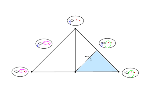
Figure 1: The metric space $\operatorname{{\cal V}}(S_{1,2})$. The fundamental domain for the action of $\operatorname{Mod}(S)$ on $\operatorname{{\cal C}}(S)$ is the union of two edges, one corresponding to a separating/nonseparating pair of curves, the other to a nonseparating/nonseparating pair. These are the only combinatorial types. Note that the latter edge has an order two symmetry, corresponding to the mapping class which switches the curves. Thus $\operatorname{{\cal V}}(S)$ is the union of a Euclidean quadrant and a quotient of a Euclidean quadrant by a reflection along the $y=x$ ray.

It is clear that Theorem 1 implies that $\operatorname{Cone}(\operatorname{{\cal M}}(S))=\operatorname{Cone}(\operatorname{{\cal V}}(S))$. Further, it is clear that multiplying the given metric on $\operatorname{{\cal V}}(S)$ by any fixed constant gives a metric space which is isometric (via the dilatation) to the original metric. In particular, $\operatorname{Cone}(\operatorname{{\cal V}}(S))$ is isometric to $\operatorname{{\cal V}}(S)$ itself. We thus deduce the following.

Corollary 2.

$\operatorname{Cone}(\operatorname{{\cal M}}(S))$ is isometric to $\operatorname{{\cal V}}(S)$.

Using different methods, Leuzinger [Le] has independently proven that $\operatorname{{\cal V}}(S)$ is bilipschitz homeomorphic to $\operatorname{Cone}(\operatorname{{\cal M}}(S))$. His methods do not seem to yield the isometry type of $\operatorname{Cone}(\operatorname{{\cal M}}(S))$.

Remarks.

1. Corollary 2 has applications to metrics of positive scalar curvature. Namely, it is a key ingredient in the proof by Farb-Weinberger that, while $\operatorname{{\cal M}}(S)$ admits a metric of positive scalar curvature for most $S$ (e.g. when $\operatorname{genus}(S)>2$), it admits no metric with the same quasi-isometry type as the Teichmüller metric on $\operatorname{{\cal M}}(S)$. See [FW].

2. For locally symmetric $M$, we know that $\operatorname{Cone}(M)$ is nonpositively curved in the ${\rm CAT}(0)$ sense. In contrast, $\operatorname{{\cal V}}(S)$ strongly exhibits aspects of positive curvature, since even within the cone on a single simplex, any two points $x,y\in\operatorname{{\cal V}}(S)$ have whole families of distinct geodesics between them, and these geodesics get arbitrarily far apart as $d(x,y)\to\infty$. This is a basic property of the $\sup$ metric on a quadrant.

3. Corollary 2 implies that any metric on $\operatorname{{\cal M}}(S)$ quasi-isometric to the Teichmüller metric must have a cone which is bilipshitz homeomorphic to $\operatorname{{\cal V}}(S)$.

The authors would like to thank the referee for some extremely helpful comments.

2 The proof of Theorem 1

2.1 Minsky’s Product Theorem

In this subsection we recall some work of Minsky which will be crucial for what follows.

Let $d=3g-3+n$. Fix $\epsilon>0$ smaller than the Margulis constant for hyperbolic surfaces. Let ${\cal C}=\{\gamma_{1},\ldots,\gamma_{p}\}$ be a collection of distinct, disjoint, nontrivial homotopy classes of simple closed curves; this is a simplex in $\operatorname{{\cal C}}(S)$. Let

$$\Omega_{\cal C}(\epsilon):=\{X\in\operatorname{\operatorname{Teich}}(S):\ell_{X}(\gamma_{i})<\epsilon\mbox{\ for each\ }i=1,\ldots,p\}.$$

Extend ${\cal C}$ to a maximal collection $\{\gamma_{1},\ldots,\gamma_{d}\}$ of homotopy classes of simple closed curves. Let $\{\theta_{i},\ell_{i})\}$ denote the corresponding Fenchel-Nielsen coordinates on $\Omega_{\cal C}(\epsilon)$. Recall that Fenchel-Nielsen coordinates give global coordinates on $\operatorname{\operatorname{Teich}}(S)$; henceforth we will identify points in $\operatorname{\operatorname{Teich}}(S)$ with their corresponding coordinates.

Consider the Teichmüller space $\operatorname{\operatorname{Teich}}(S\setminus{\cal C})$, which is the space of complete, finite area hyperbolic metrics on $S\setminus{\cal C}$. Note that the coordinates $\{(\theta_{i},\ell_{i}):i>p\}$ give Fenchel-Nielsen coordinates on $\operatorname{\operatorname{Teich}}(S\setminus{\cal C})$.

Let

$$\Phi=(\Phi_{1},\Phi_{2}):\Omega_{\cal C}(\epsilon)\to\operatorname{\operatorname{Teich}}(S\setminus{\cal C})\times\prod_{i=1}^{p}\mbox{\bf H}^{2}$$

be defined by

$$\Phi((\theta_{1},\ldots,\theta_{d},\ell_{1},\ldots,\ell_{d},)):=(\theta_{p+1},\ldots,\theta_{d},\ell_{p+1},\ldots,\ell_{d},)\times\prod_{i=1}^{p}(\theta_{i},1/\ell_{i}).$$

Notice that we are changing the last set of length coordinates from $\ell$ to $1/\ell$ giving coordinates in the upper half-space model of $\mbox{\bf H}^{2}$. We give $\mbox{\bf H}^{2}$ the metric $ds^{2}=\frac{1}{4}(dx^{2}+dy^{2})/y^{2}$. Note that the factor of $\frac{1}{4}$ leads to a factor of $\frac{1}{2}$ in the distance, and is consistent with the factor of $\frac{1}{2}$ in the metric on the Euclidean octant. If $S\setminus{\cal C}$ is disconnected, then $\operatorname{\operatorname{Teich}}(S\setminus{\cal C})$ is itself a product of the Teichmuller spaces of the components of $S\setminus{\cal C}$; we endow this total product space itself with the $\sup$ metric, denoted by $d$. We remark that $\Phi$ is a homeomorphism onto its image, and its image is $\operatorname{\operatorname{Teich}}(S\setminus{\cal C})\times\prod_{i=1}^{p}\{(x_{i},y_{i})\in\mbox{\bf H}^{2}:y_{i}>1/\epsilon\}$.

The following was proved in [Mi].

Theorem 3 (Minsky Product Theorem).

With notation as above, there exists $D$ such that for all $X,Y\in\Omega_{\cal C}(\epsilon)$,

$$|d(\Phi(X),\Phi(Y))-d_{\operatorname{\operatorname{Teich}}(S)}(X,Y)|\leq D.$$

We will need the following lemma about distances in $\operatorname{{\cal M}}(S)$.

Lemma 4.

Given constants $C,C^{\prime}$ there is a constant $C^{\prime\prime}$ with the following property. Let $\sigma=\{\alpha_{1},\ldots,\alpha_{d}\}$ be a maximal simplex of $\widetilde{V}(S)$. Let $X,Y\in\operatorname{\operatorname{Teich}}(S)$ be such that $\ell_{X}(\alpha_{i})\leq C$ and $\ell_{Y}(\alpha_{i})\leq C$ for each $i$. Suppose also that $|\log(\ell_{X}(\alpha_{i})/\ell_{Y}(\alpha_{i}))|\leq C^{\prime}$. Then $d_{\operatorname{{\cal M}}(S)}(\pi(X),\pi(Y))\leq C^{\prime\prime}$.

Proof. This follows from Theorem 3. We can find a point $Y^{\prime}$ which differs from $Y$ by Dehn twists about curves in $\sigma$ so that the Fenchel-Nielsen twist coordinates of $X,Y^{\prime}$ have bounded difference. Now we consider the list of curves shorter than $\epsilon$ on both $X$ and $Y^{\prime}$. Since the ratios of lengths of these short curves are bounded above, as are the differences in twist coordinates, it follows that the distances in the corresponding $\mbox{\bf H}^{2}$ factors are bounded. The complement of these short curves determines a boundary Teichmuller space. The lengths of the remaining curves are bounded above and below, giving that the surfaces have a bounded distance from each other in this boundary Teichmüller space. The existence of $C^{\prime\prime}$ now follows from Theorem 3. $\diamond$

2.2 Defining the map $\Psi$

We will define a map $\widetilde{\Psi}:\widetilde{\operatorname{{\cal V}}}(S)\to\operatorname{{\cal M}}(S)$ by giving its value on a representative of each $\operatorname{Mod}(S)$-orbit in $\widetilde{\operatorname{{\cal V}}}(S)$, and then define $\widetilde{\Psi}$ to be constant on orbits. It will then follow that $\widetilde{\Psi}$ induces a map $\Psi:\operatorname{{\cal V}}(S)\to\operatorname{{\cal M}}(S)$. While this map will not be continuous, we will prove that it is a $(1,D)$-quasi-isometry for some $D\geq 0$.

Fix a (finite) collection of maximal simplices that represent all combinatorial types. We will first define $\widetilde{\Psi}$ on the open cone over this collection. Thus let $\sigma$ be one of these maximal simplices of $\operatorname{{\cal C}}(S)$ representing a maximal collection of disjoint simple closed curves $\{\alpha_{1},\ldots,\alpha_{d}\}$. Again we think of the cone on $\sigma$, as a subspace of $\widetilde{\operatorname{{\cal V}}}(S)$, as an octant in $\mbox{\bf R}^{d}$ with coordinates $x_{1},\ldots,x_{d}$, endowed with the $\sup$ metric. Let $\operatorname{Mod}(S,\sigma)$ be the subgroup of $\operatorname{Mod}(S)$ that fixes $\sigma$. It acts on the open cone over $\sigma$ with finite orbit. Take a sector $\Lambda(\sigma)$ inside this cone which is a fundamental domain for the action of $\operatorname{Mod}(S,\sigma)$. For any $(x_{1},\ldots,x_{d})\in\Lambda(\sigma)$ (no $x_{i}=0$), let

$$\widetilde{\Psi}(x_{1},\ldots,x_{d}):=\pi(X)$$ (1)

where $\pi(X)$ is any point of $\pi(\Omega_{\sigma}(\epsilon))$ such that

$$\ell_{X}(\alpha_{i})=\epsilon e^{-x_{i}}\ \ \mbox{for each $i$}.$$

Using the action of $\operatorname{Mod}(S,\sigma)$ we extend $\widetilde{\Psi}$ to the entire open cone on $\sigma$. Note that $\widetilde{\Psi}$ is continuous on each open cone. We do this for each maximal cone in the finite collection. Now use the action of $\operatorname{Mod}(S)$ to extend $\widetilde{\Psi}$ to the open cones on all maximal simplices by having it be constant on orbits.

Next let $\tau$ be a simplex which is not maximal. Choose some closed maximal simplex $\sigma=\sigma(\tau)$ containing $\tau$. We call this the maximal simplex associated to $\tau$. The cone on $\tau$ is given by the coordinates $(x_{1},\ldots,x_{d})$ for the cone on $\sigma$ as above. The coordinates $x_{i}$ corresponding to curves in $\sigma-\tau$ are set to $0$. Define $\widetilde{\Psi}$ on $\tau$ via the equation (1) above. Thus all curves in $\sigma-\tau$ are assigned the fixed length $\epsilon$ while the curves in $\tau$ can have arbitrarily small length. We extend $\widetilde{\Psi}$ to all of $\widetilde{\operatorname{{\cal V}}}(S)$ by declaring $\widetilde{\Psi}$ to be constant on each $\operatorname{Mod}(S)$-orbit in $\widetilde{\operatorname{{\cal V}}}(S)$. It follows that $\widetilde{\Psi}$ induces a map $\Psi:\operatorname{{\cal V}}(S)\to\operatorname{{\cal M}}(S)$. We remark that $\Psi$ will in general not be continuous because of the choices made at a face of a maximal simplex. Nonetheless we want to know that the jump in the function at any face is uniformly bounded. We will argue this below using Lemma 4 together with the following lemma.

Lemma 5.

Let $\tau$ be a simplex. Let $\sigma_{1}$ a maximal simplex associated to $\tau$ and let $\sigma_{2}$ be any other maximal simplex such that $\tau=\sigma_{1}\cap\sigma_{2}$. Then there exists an element $\phi\in\operatorname{Mod}(S)$, fixing $\tau$, such that for each $x$ in the cone over $\tau$ there is a point $X\in\operatorname{\operatorname{Teich}}(S)$ with $\pi(X)=\widetilde{\Psi}(x)$ and such that the $X$-length of any curve in $(\sigma_{1}-\tau)\cup(\phi(\sigma_{2})-\tau)$ is bounded above by a universal constant, and below by the fixed $\epsilon$.

Proof. The coordinates for curves in $\sigma_{1}-\tau$ on the cone over $\tau$ are $0$. By definition, each curve $\beta\in\sigma_{1}-\tau$ then has fixed length $\epsilon$ on some $X$ with $\pi(X)=\widetilde{\Psi}(x)$. The curves in $\sigma_{2}-\tau$ may have large intersection with curves in $\sigma_{1}-\tau$ and therefore large length on $X$. However, since there are only finitely many combinatorial types of pants decompositions, we can choose $\phi$ fixing $\tau$ so that any curve in $\phi(\sigma_{2})-\tau$ has universally bounded intersection with any curve in $\sigma_{1}-\tau$. Since $\ell_{X}(\beta)=\epsilon$ for each $\beta\in\sigma_{1}-\tau$, the collar about $\beta$ has diameter bounded above. Thus we can further compose $\phi$ by Dehn twists about $\beta$, so that for the new $\phi$, the curves in $\phi(\sigma_{2})-\tau$ have bounded lengths on $X$. $\diamond$

2.3 Properties of $\Psi$

Our goal in this subsection is to prove that $\Psi$ is a $(1,D)$-quasi-isometry. In order to do this we will need the following setup.

Let $\sigma$ a maximal simplex. Recall $P$ is the quotient map from $\operatorname{{\cal C}}(S)$ to $\operatorname{{\cal C}}(S)/\operatorname{Mod}(S)$. Let $d_{P(\sigma)}$ be the path metric on the cone over $P(\sigma)$ and let $d^{\operatorname{{\cal M}}(S)}_{P(\sigma)}$ be the path metric on the (connected) $\Psi$ image of the cone over $P(\sigma)$ in $\operatorname{{\cal M}}(S)$ induced from the Teichmüller metric on $\operatorname{{\cal M}}(S)$. That is, the distance between two points in the image is the infimum of the lengths of paths joining the points that stays in the image of the cone over $P(\sigma)$.

Lemma 6.

There is a constant $D_{0}$ such that if $x_{1},x_{2}$ lie in the cone over $P(\sigma)$, then

$$|d_{P(\sigma)}(x_{1},x_{2})-d_{P(\sigma)}^{\operatorname{{\cal M}}(S)}(\Psi(x_{1}),\Psi(x_{2}))|\leq D_{0}.$$

Proof. We may find a lift $X_{i}$ of $\Psi(x_{i})$ to $\operatorname{\operatorname{Teich}}(S)$ such that the difference of the twist coordinates of $X_{1}$ and $X_{2}$ with respect to the Fenchel-Nielsen coordinates defined by $\sigma$ are bounded and such that

$$d_{\operatorname{\operatorname{Teich}}(S)}(X_{1},X_{2})=d_{P(\sigma)}^{\operatorname{{\cal M}}(S)}(\Psi(x_{1}),\Psi(x_{2})).$$

If $x_{1}$ and $x_{2}$ lie in the open cone over $P(\sigma)$, then the lemma follows from Theorem 3 and the definition of the metric $d_{P(\sigma)}$. If not, then one must further quote Lemma 5 and Lemma 4. $\diamond$

$\Psi$ is almost onto: By a theorem of Bers, there is a constant $C=C(g,n)$ such that each $X\in\operatorname{\operatorname{Teich}}(S)$ has a pants decomposition corresponding to a maximal simplex $\sigma$ such that each curve of $\sigma$ has length at most $C$ on $X$. With respect to these pants curves, each of the twist coordinates is bounded, modulo the action of Dehn twists about the curves in $\sigma$, by $2\pi C$. Let $\tau$ be the possibly empty face of $\sigma$ such that the set of curves in $\sigma-\tau$ have lengths on $X$ between $\epsilon$ and $C$. The curves in $\tau$ have length at most $\epsilon$. By Lemma 5, there is a point $Y\in\operatorname{\operatorname{Teich}}(S)$ such that $\pi(Y)$ is in the $\Psi$-image of the cone on $\tau$, and such that the lengths on $Y$ of the curves in $\tau$ are the same as the lengths on $X$ of those curves, and the curves in $\sigma-\tau$ have bounded length on $Y$. Thus their ratios to the lengths on $X$ are bounded. Applying Lemma 4, we are done.

$\Psi$ is an almost isometry: We need the following lemma.

Lemma 7 (Path Lemma).

The following statements are true.

1. Any two points in $\operatorname{{\cal V}}(S)$ can be joined by a geodesic that enters the cone over each $P(\sigma)$, where $\sigma$ is a maximal simplex of $\widetilde{V(S)}$, at most once.

2. There is a constant $C^{\prime}$ such that any two points of $\Psi(\operatorname{{\cal V}}(S))$ can be joined by a $(1,C^{\prime})$ quasi-geodesic in the metric $d_{\operatorname{{\cal M}}(S)}$ that enters the cone over each $P(\sigma)$ at most once.

A first step in proving Lemma 7 is the following.

Lemma 8.

The following statements are true.

1. Suppose $x,y$ are points in the cone over $P(\sigma)$ where $\sigma$ is a maximal simplex. Then there is a geodesic joining $x$ and $y$ that stays in the cone over that $P(\sigma)$.

2. There is a constant $C^{\prime\prime}$ such that if $\Psi(x),\Psi(y)$ lie in the cone over $P(\sigma)$ then

   $$d_{P(\sigma)}^{\operatorname{{\cal M}}(S)}(\Psi(x),\Psi(y))\leq d_{\operatorname{{\cal M}}(S)}(\Psi(x),\Psi(y))+C^{\prime\prime}.$$

We note that the opposite inequality

$$d_{\operatorname{{\cal M}}(S)}(\Psi(x),\Psi(y))\leq d_{P(\sigma)}^{\operatorname{{\cal M}}(S)}(\Psi(x),\Psi(y))$$

is clearly true.

Proof. [of Lemma 8] We prove the first statement. Lift to $\widetilde{\operatorname{{\cal V}}}(S)$ and consider again $x,y$ with the same names such that the distance in the cone over $\sigma$ realizes the distance between $x$ and $y$ in the cone over $P(\sigma)$. Let the coordinates of $x,y$ be given by $(x_{1},\ldots,x_{d}),(y_{1},\ldots,y_{d})$. Suppose $\sigma$ is defined by the curves $\alpha_{1},\ldots,\alpha_{d}$ of a pants decomposition. Without loss of generality assume that $d_{\sigma}(x,y)=\frac{1}{2}(y_{1}-x_{1})$. We must show that, for every $\phi\in\operatorname{Mod}(S)$, that does not fix $\sigma$, there is no shorter path $\rho$ in $\widetilde{\operatorname{{\cal V}}}(S)$ from $\phi(x)$ to $y$.

Suppose first that $\alpha_{1}$ is not a vertex in the simplex $\phi(\sigma)$. Then the path from $x$ to $y$ for a last time must enter the cone over a simplex for which $\alpha_{1}$ is a vertex at a point $z$. At $z$ the coordinate corresponding to $\alpha_{1}$ is $0$, and so

$$d_{\operatorname{{\cal V}}(S)}(y,z)\geq y_{1}/2\geq d_{\sigma}(x,y).$$

Thus we may assume that the path $\rho$ joining $\phi(x)$ to $y$ lies completely in the cones over simplices for which $\alpha_{1}$ is a vertex. Break up this path into segments $\rho=\rho_{1}*\rho_{2}*\ldots*\rho_{N}$, where each $\rho_{i}$ lies in the cone over a single simplex. Let $z_{1}^{i}$ (resp. $z_{1}^{i+1}$) be the coordinate of $\alpha_{1}$ at the beginning (resp. end) of $\rho_{i}$, where $z_{1}^{1}=x_{1}$ and $z_{1}^{N+1}=y_{1}$. Then $|\rho_{i}|\geq\frac{1}{2}|z_{1}^{i+1}-z_{1}^{i}|$. Thus

$$|\rho|=\sum_{i=1}^{N}|\rho_{i}|\geq\sum\frac{1}{2}|z_{1}^{i+1}-z_{1}^{i}|\geq\frac{1}{2}(y_{1}-x_{1})=d_{\widetilde{V}(S)}(x,y).$$

We conclude that a shortest path can be found by a geodesic that lies entirely in the cone over $\sigma$

We prove the second statement. First lift $\Psi(x),\Psi(y)$ to elements $X,Y\in\operatorname{\operatorname{Teich}}(S)$ which lie in $\Omega_{\sigma}(\epsilon)$, and such that

$$d_{P(\sigma)}^{\operatorname{{\cal M}}(S)}(\Psi(x),\Psi(y))=d_{\operatorname{\operatorname{Teich}}(S)}(X,Y)$$

and whose twist coordinates are bounded by $2\pi\epsilon$. By Theorem 3, there exists a simple closed curve $\alpha_{1}\in\sigma$ such that

$$|d_{\operatorname{\operatorname{Teich}}(S)}(X,Y)-\frac{1}{2}\log(\ell_{Y}(\alpha_{1})/\ell_{X}(\alpha_{1}))|\leq D^{\prime}$$

where $D^{\prime}$ depends on $\epsilon$ and on the constant $D$ from Theorem 3. Thus

$$|d_{P(\sigma)}^{\operatorname{{\cal M}}(S)}(\Psi(x),\Psi(y))-\frac{1}{2}\log(\ell_{Y}(\alpha_{1})/\ell_{X}(\alpha_{1}))|\leq D^{\prime}.$$ (2)

Now let $\phi$ be a mapping class group element. If $\alpha_{1}$ is not a vertex of $\phi(\sigma)$ then any path $\rho$ from $\phi(Y)$ to $X$ must enter a set $\Omega_{\cal C}(\epsilon)$ for some $\cal C$ containing $\alpha_{1}$ a last time. At that time the length of $\alpha_{1}$ is $\epsilon$. By Theorem 3 and Equation (2) we then have

$$|\rho|\geq\frac{1}{2}\log(\epsilon/\ell_{X}(\alpha_{1}))-D\geq d_{P(\sigma)}^{\operatorname{{\cal M}}(S)}(\Psi(y),\Psi(x))+\frac{1}{2}\log(\epsilon/\ell_{Y}(\alpha_{1}))-D-D^{\prime}.$$

Since $\ell_{Y}(\alpha_{1})$ is bounded above, the term $\frac{1}{2}\log(\epsilon/\ell_{Y}(\alpha_{1}))-D-D^{\prime}$ is bounded below by some constant, and we set $-C^{\prime\prime}$ to be this constant.

Thus again we can assume that $\rho$ lies completely in $\Omega_{\cal C}(\epsilon)$ for a set $\cal C$ containing $\alpha_{1}$. But now the conclusion again follows from Theorem 3. $\diamond$

Proof. [of Lemma 7] Suppose $x$ is in the cone over $P(\sigma_{1})$ and that $y$ is in the cone over $P(\sigma_{2})$. If $P(\sigma_{1})=P(\sigma_{2})$ then we are done by Lemma 8. Thus we can assume that $P(\sigma_{2})\neq P(\sigma_{1})$. Suppose $\rho$ is a geodesic from $x$ to $y$. Suppose $\rho$ leaves the cone over $P(\sigma_{1})$ and returns to it for a last time at some $z$ in the cone over $P\sigma_{1})\cap P(\sigma_{3})$ for some maximal simplex $\sigma_{3}$. Then by the first part of Lemma 8 we can replace $\rho$ by a geodesic that stays in the cone over $P(\sigma_{1})$ from $x$ to $z$ and then follows $\rho$ from $z$ to $y$ never returning to the cone over $P(\sigma_{1})$. We now find the last point $w$ that lies in the cone over $P(\sigma_{3})$ and replace a segment of $\rho$ with one that stays in the cone over $P(\sigma_{3})$ and never returns again to the cone over $P(\sigma_{3})$. Since there are only a finite number of simplices in $\operatorname{{\cal C}}(S)/\operatorname{Mod}(S)$, continuing to apply Lemma 8, we are done. This proves the first statement.

The proof of the second statement is similar, where we now use the second part of Lemma 8. $\diamond$

We now continue with the final step in the proof of Theorem 1, that the map $\Psi$ is an almost isometry. We first prove that

$$d_{\operatorname{{\cal M}}(S)}(\Psi(x),\Psi(y))\leq d_{\operatorname{{\cal V}}(S)}(x,y)+R$$

for some constant $R$. To prove this, consider a geodesic path $\gamma\subset\operatorname{{\cal V}}(S)$ connecting $x$ to $y$. By the first statement of Lemma 7, there exists $c=c(S)$ so that $\gamma$ can be written as a concatenation $\gamma=\gamma_{1}\ast\cdots\ast\gamma_{c}$ with each $\gamma_{i}$ a geodesic in the cone over $P(\sigma)$ for $\sigma$ a maximal simplex $\sigma_{i}$ of $\operatorname{{\cal V}}(S)$. By Lemma 6 each $\Psi(\gamma_{i})$ is a $(1,D_{0})$-quasigeodesic in the metric $d_{\operatorname{{\cal M}}(S)}$. It follows that $\Psi(\gamma)$ is a $(1,cD^{\prime})$-quasigeodesic.

The proof of the opposite inequality

$$d_{\operatorname{{\cal V}}(S)}(x,y)\leq d_{\operatorname{{\cal M}}(S)}(\Psi(x),\Psi(y))+R^{\prime}$$

for some $R^{\prime}$ uses the second conclusion of Lemma 7. Any two points can be joined by $(1,C^{\prime})$ quasi-geodesic in the metric $d_{\operatorname{{\cal M}}(S)}$ and which intersects a fixed number of cones over image simplices $P(\sigma)$. We now apply Lemma 6 to conclude that $d_{\operatorname{{\cal V}}(S)}(x,y)$ is only larger by an additive constant.

Dept. of Mathematics, University of Chicago
5734 University Ave.
Chicago, Il 60637
E-mail: farb@math.uchicago.edu, masur@math.uchicago.edu

References

• [FW] B. Farb and S. Weinberger, Positive scalar curvature metrics on the moduli space of Riemann surfaces, in preparation.
• [Ha1] T. Hattori, Collapsing of quotient spaces of ${\rm SO}(n)\backslash{\rm SL}(n,R)$ at infinity, J. Math. Soc. Japan 47 (1995), no. 2, 193–225.
• [Ha2] T. Hattori, Asymptotic geometry of arithmetic quotients of symmetric spaces, Math. Zeit. 222 (1996), no. 2, 247–277.
• [JM] L. Ji and R. MacPherson, Geometry of compactifications of locally symmetric spaces, Ann. Inst. Fourier, Grenoble, Vol. 52, No. 2 (2002), 457–559.
• [Le] E. Leuzinger, Reduction theory for mapping class groups, preprint, Jan. 2008.
• [Mi] Y. Minsky, Extremal length estimates and product regions in TeichmΓΌller space, Duke Math. Jour. 83 (1996), no. 2, 249–286.