Wigner symmetry, Large $N_{c}$ and Renormalized One Boson Exchange Potentials.

Abstract

Wigner symmetry in Nuclear Physics provides a unique example of a non-perturbative long distance symmetry, a symmetry strongly broken at short distances. We analyse the consequences of such a concept within the framework of One Boson Exchange Potentials in NN scattering and keeping the leading $N_{c}$ contributions. Phenomenologically successful relations between singlet ${}^{1}S_{0}$ and triplet ${}^{3}S_{1}$ scattering phase shifts are provided in the entire elastic region. We establish symmetry breaking relations among non-central phase shifts which are successfully fulfilled by even-L partial waves and strongly violated by odd-L partial waves, in full agreement with large $N_{c}$ requirements.

I Introduction

Symmetries have traditionally been very useful in nuclear physics partly because the force at the hadronic level is not well known at short distances Wigner and Feenberg (1941); Wilkinson (1969); Van Isacker (1999). In some cases, like isospin, chiral or heavy quark symmetry, the invariance can directly be traced from the fundamental QCD Lagrangean and formulated in terms of the underlying quark and gluonic degrees of freedom. In some other cases the connection is less straightforward. Many years ago Wigner and Hund proposed Wigner (1937); Hund (1937) extending the spin and isospin $SU_{S}(2)\otimes SU_{I}(2)$ symmetry into the larger $SU(4)$ group where the nucleon-spin states $p\uparrow$, $p\downarrow$, $n\uparrow$, $n\downarrow$ correspond to the fundamental representation, and hence providing a supermultiplet structure of nuclear energy levels as well as new selection rules for nuclear transitions and response functions Donnelly and Walker (1970). The corresponding $SU(4)$ mass formula was found to be at least as good as the well known Weizsäcker one  Cauvin et al. (1981); Van Isacker et al. (1997). Spin-orbit interaction of the shell model obviously violate the symmetry, and indeed a breakdown of $SU(4)$ has been reported for heavier nuclei Vogel and Ormand (1993) while nuclear matter has been addressed in Nayak and Kota (2001). Double binding energy differences have been shown to be a useful test of the symmetry Van Isacker et al. (1995). Recently, inequalities for light nuclei based on $SU(4)$ and Euclidean path integrals have been derived by neglecting all but S-wave interactions Chen et al. (2004).

Despite its relative success along the years, $SU(4)$ symmetry has been treated as an accidental one within the traditional approach to Nuclear Physics and guessing its origin from QCD has been a subject of some interest in the last decade. Indeed, attempts to justify $SU(4)$ spin-flavour symmetry from a more fundamental level have been carried out along several lines. Based on the limit of large number of colors $N_{c}$ of QCD ’t Hooft (1974); Witten (1979), it was shown Kaplan and Savage (1996); Kaplan and Manohar (1997) that if the nucleon momentum scales as $p\sim N_{c}^{0}$, the nuclear potentials scale either as $N_{c}$ or $1/N_{c}$, depending upon the particular spin-isospin channel, which shows that the NN force could be determined with $1/N_{c}^{2}$ relative accuracy. It was found that the leading potential would be $SU(4)$ symmetric if the tensor force was neglected in addition, a plausible assumption for light nuclei where S-waves dominate. Although these estimates are conducted directly in terms of quarks and gluons, quark-hadron duality allows to reformulate these results in terms of purely hadronic degrees of freedom, providing a rationale for the One-Boson-Exchange (OBE) potential models Machleidt et al. (1987), and the internal consistency of Two- Banerjee et al. (2002) and Multiple Boson Exchanges Belitsky and Cohen (2002); Cohen (2002). The analysis of sizes of volume integrals of phenomenologically successful potentials confirms the large $N_{c}$ expectations Riska (2002). The large size of scattering lengths was regarded as a fingerprint of the $SU(4)$ symmetry within an Effective Field Theory (EFT) viewpoint Mehen et al. (1999) using the Power Divergent Subtracted (PDS) scheme; singlet and triplet renormalized couplings coincide at the natural renormalization scale $\mu\sim m_{\pi}\gg 1/\alpha_{s},1/\alpha_{t}$, with $\alpha_{s}$ and $\alpha_{t}$ the scattering lengths, and a contact interaction makes sense in such a scaling regime. Resonance saturation based on the elimination of exchanged mesons in the OBE Bonn potential Machleidt et al. (1987) at very low energies was also shown to reproduce the EFT approach and to agree numerically with the Wigner symmetry expectations Epelbaum et al. (2002). According to Refs. Epelbaum et al. (2003); Beane and Savage (2003); Braaten and Hammer (2003); Epelbaum et al. (2006); Hammer et al. (2007) QCD might be close to a point where the effective theory had an $SU(4)$ symmetry at zero energy as well as discrete scale invariance if the pion mass was larger than its physical value, around $m_{\pi}\sim 200{\rm MeV}$. This nice idea might be confirmed by recent fully dynamical lattice QCD determinations of the scattering lengths Beane et al. (2006) and quenched lattice QCD evaluations of NN potentials Ishii et al. (2007); Aoki et al. (2008) where indeed unphysical pion masses are probed.

While the proclaimed symmetry holds in a range where scale invariance sets in and EFT methods based on contact interactions can be applied Mehen et al. (1999); Epelbaum et al. (2002), is not obvious what are the implications for the lightest NN system itself for finite energies and for physical pion masses. In particular, the scale dependence of the contact interaction is modified when the finite range of the long distance potential is taken into account. To be specific, low energy NN scattering is dominated by S-waves in different $(S,T)$ channels where spin and isospin are interchanged, $(1,0)$=${}^{1}S_{0}\leftrightarrow(0,1)$= ${}^{3}S_{1}$. Wigner $SU(4)$ symmetry predicts identical interactions in both ${}^{1}S_{0}$ and ${}^{3}S_{1}$ channels. The above mentioned identity of the ${}^{1}S_{0}$ and ${}^{3}S_{1}$ potentials holds also in the large $N_{c}$-expansion Kaplan and Savage (1996); Kaplan and Manohar (1997), so we take advantage of this fact by using the leading $N_{c}$-OBE potentials which simplifies the discussion to a large extent as we discuss in Sect. II. In contrast, the corresponding phase shifts from Partial Wave Analyses Stoks et al. (1993) are very different at all energies. We are thus confronted with an intriguing puzzle since it is not obvious at all in what sense should the symmetry be interpreted for the NN system; it would be difficult to understand otherwise the successes of $SU(4)$ for light nuclei. A second puzzle arises from an embarrasing cohabitation of conflicts and agreements between large-$N_{c}$ studies and Wigner symmetry. Despite the initial claim Kaplan and Savage (1996) a more complete analysis Kaplan and Manohar (1997) could only justify the Wigner symmetry in even-L partial waves while for odd-L a violation of the symmetry was expected. However, doing so required neglecting the tensor force, which according to the Wigner symmetry should vanish, but it is a leading contribution to the potential in the large $N_{c}$ limit. Thus, while some pieces of the NN potential (such as e.g. spin-orbit) are suppressed in both schemes, some others are not simultaneously small. These conflicts between the time-honoured $SU(4)$ Wigner symmetry and the QCD based large-$N_{c}$ expansion for odd-L channels require an explanation and naturally pose the question on the validity of either framework.

In the present work we analyze both puzzles by introducing the concept of a long distance symmetry firstly to understand the meaning of Wigner symmetry in those cases where its validity complies with large $N_{c}$ expectations. This is a case where we expect the symmetry to be more robust. Once this is done, it is pertinent to dilucidate the validity of the symmetry in those cases where a possible conflict with the large $N_{c}$ expansion arises. Our discussion is tightly linked to the coordinate space renormalization discussed in previous works Pavon Valderrama and Arriola (2006, 2007). This approach while borrowing the physical motivation from EFT theories provides a quantum mechanical framework where the emphasis is placed on the non-perturbative aspects of the NN problem, a playground where the standard EFT viewpoint has encountered notorious difficulties. The method is reviewed in Sect. III for completeness. We find that for S-waves the Wigner symmetry holds in a much wider range than the applicability of a contact interaction suggests if the finite range of the interaction is incorpored. As a byproduct we provide in Sect. IV quantitative predictions; the seemingly independent triplet and singlet S-waves phase shifts corresponding to iso-vector and iso-scalar states respectively for the np system are shown to be neatly intertwined in the entire elastic region. A similar correlation can also be established between the ${}^{1}S_{0}$ virtual state and the ${}^{3}S_{1}$ deuteron bound state. Actually, we show how the symmetry may be visualized for large scattering lengths due to the onset of scale invariance. Symmetry breaking due to inclusion of further counter-terms, tensor interaction and spin-orbit interaction are discussed in Sect. V. We show how a sum rule for supermultiplet phase shifts splitting due to spin-orbit and tensor interactions is well fulfilled for non-central L-even waves, and strongly violated in L-odd waves where a Serber-like symmetry holds instead. This pattern of $SU(4)$-symmetry breaking complies to the large $N_{c}$ expectations, a somewhat unexpected conclusion. Finally, in Sect. VI we provide our main conclusions and outlook for further work.

II OBE potentials, Large $N_{c}$ and Wigner symmetry

Our starting point is the field theoretical OBE model of the NN interaction Machleidt et al. (1987) which includes all mesons with masses below the nucleon mass, i.e., $\pi$, $\sigma(600),$$\eta$, $\rho(770)$ and $\omega(782)$. For the purpose of discussing $SU(4)$ Wigner symmetry within the OBE framework (see Appendix A for a brief overview) we will deal here with S-waves only, neglecting for the moment the S-D wave mixing stemming from the tensor force as required by Wigner symmetry. Our results of Sect. IV and estimates in Sect. V.2 will provide the a posteriori justification of this simplifying assumption. Non-central waves and the role of spin-orbit as well as tensor force will be treated in Sect. V.3 as $SU(4)$-breaking perturbations. For the S-waves the NN potential reads

$$V=V_{C}+\tau W_{C}+\sigma V_{S}+\tau\sigma W_{S}\,,$$ (1)

where $\tau=\tau_{1}\cdot\tau_{2}=2T(T+1)-3$ and $\sigma=\sigma_{1}\cdot\sigma_{2}=2S(S+1)-3$ and Pauli principle requires $(-)^{S+T+L}=-1$. Thus, for the spin singlet ${}^{1}S_{0}$ and spin triplet ${}^{3}S_{1}$ states we get

$$V_{s} = V_{C}+W_{C}-3V_{S}-3W_{S}\,,$$ (2)

$$V_{t} = V_{C}-3W_{C}+V_{S}-3W_{S}\,,$$ (3)

To simplify the discussion we will discard terms in the potential which are phenomenologically small. Actually, according to Refs. Kaplan and Savage (1996); Kaplan and Manohar (1997) in the leading large $N_{c}$ one has $V_{C}\sim W_{S}\sim N_{c}$ while $V_{S}\sim W_{C}\sim 1/N_{c}$. In terms of meson exchanges (see also Ref. Banerjee et al. (2002)) one has the contributions

$$V_{s}(r)=V_{t}(r) = -\frac{g_{\pi NN}^{2}m_{\pi}^{2}}{16\pi M_{N}^{2}}\frac{e^{-m_{\pi}r}}{r}-\frac{g_{\sigma NN}^{2}}{4\pi}\frac{e^{-m_{\sigma}r}}{r}$$ (4)

$$+ \frac{g_{\omega NN}^{2}}{4\pi}\frac{e^{-m_{\omega}r}}{r}-\frac{f_{\rho NN}^{2}m_{\rho}^{2}}{8\pi M_{N}^{2}}\frac{e^{-m_{\rho}r}}{r}$$

$$+ {\cal O}\left({N_{c}}^{-1}\right)\,,$$

where $g_{\sigma NN}$ is a scalar type coupling, $g_{\pi NN}$ a pseudo-scalar derivative coupling, $g_{\omega NN}$ is a vector coupling and $f_{\rho NN}$ the tensor derivative coupling (see Machleidt et al. (1987) for notation). Here, the scheme proposed in Partovi and Lomon (1970) of neglecting both energy and nonlocal corrections is realized explicitly. In principle the large $N_{c}$ limit contains infinitely many multi-meson exchanges which decay exponentially with the sum of the exchanged meson masses. However, NN scattering in the elastic region below pion production threshold probes CM momenta $p<p_{max}=400$ MeV. Given the fact that $1/m_{\omega}=0.25\mathrm{fm}\ll 1/p_{max}=0.5\mathrm{fm}$ we expect heavier meson scales to be irrelevant, an in particular $\omega$ and $\rho$ themselves, are expected to be at most marginally important . Note that, in any case, when $m_{\omega}=m_{\rho}$ the redundant combination $g_{\omega NN}^{2}-f_{\rho NN}^{2}m_{\rho}^{2}/(2M_{N}^{2})$ appears, indicating a further source of cancellation between $\rho$ and $\omega$ in this channel. Moreover, since the leading contributions to the potential are $\sim N_{c}$ and the subleading ones are $\sim 1/N_{c}$, the neglected terms are of relative $1/N_{c}^{2}$ order, so we might expect an a priori $\sim 10\%$, accuracy.

The coincidence between ${}^{1}S_{0}$ and ${}^{3}S_{1}$ potentials complies to the Wigner $SU(4)$ symmetry which we review for completeness in Appendix A for the two-nucleon system. Modern high quality potentials Stoks et al. (1994) describing accurately NN scattering below pion production threshold show some traces of the symmetry for distances above $1.4-1.8{\rm fm}$. Quenched lattice QCD evaluations of NN potentials for $m_{\pi}/m_{\rho}\sim 0.6$ Ishii et al. (2007); Aoki et al. (2008) yield also similar ${}^{1}S_{0}$ and ${}^{3}S_{1}$ potentials for $r>1.4{\rm fm}$. Thus, at first sight one may conclude that Wigner symmetry holds when OPE dominates, and thus has a limited range of applicability. An important result of the present investigation, which will be elaborated along the paper, is that this is not necessarily so, provided the relevant scales of symmetry breaking are properly isolated with the help of renormalization ideas.

Let us analyze the consequences of the symmetry, Eq. (4), within the standard approach to OBE potentials. The scattering phase-shift $\delta_{0}(p)$ is computed by solving the (S-wave) Schrödinger equation in r-space

$$-u^{\prime\prime}_{p}(r)+M_{N}\,V(r)\,u_{p}(r) = p^{2}\,u_{p}(r)\,,$$ (5)

$$u_{p}(r) \to \frac{\sin{\left(pr+\delta_{0}(p)\right)}}{\sin{\delta_{0}(p)}}\,,$$ (6)

with a regular boundary condition at the origin $u_{p}(0)=0$. Moreover, for a short range potential such as the one in Eq. (4) one also has the Effective Range Expansion (ERE)

$$p\cot{\delta_{0}(p)}=-\frac{1}{\alpha_{0}}+\frac{1}{2}\,r_{0}\,p^{2}+\cdots\,,$$ (7)

where the scattering length, $\alpha_{0}$, is defined by the asymptotic behavior of the zero energy wave function as

$$u_{0}(r) \to 1-\frac{r}{\alpha_{0}}\,,$$ (8)

and the effective range, $r_{0}$, is given by

$$r_{0} = 2\int_{0}^{\infty}dr\left[\left(1-\frac{r}{\alpha_{0}}\right)^{2}-u_{0}(r)^{2}\right]\,.$$ (9)

In the usual approach Machleidt et al. (1987); Machleidt (2001) everything is obtained from the potential assumed to be valid for $0\leq r<\infty$. We note incidentally that the Wigner symmetry relation, Eq. (4), holds at all distances . In addition, due to the unnaturally large NN ${}^{1}S_{0}$ scattering length ($\alpha_{s}\sim-23{\rm fm}$), any change in the potential $V\to V+\Delta V$ has a dramatic effect on $\alpha_{0}$, since one obtains

$$\Delta\alpha_{0}=\alpha_{0}^{2}M_{N}\int_{0}^{\infty}\Delta V(r)u_{0}(r)^{2}\mathrm{d}r\,,$$ (10)

and thus the potential parameters must be fine tuned, and in particular the short distance physics. As it was discussed in Refs. Ruiz Arriola et al. (2007); Calle Cordon and Ruiz Arriola (2008) this short distance sensitivity is unnatural as long as the OBE potential does not truely represent a fundamental NN force at short distances. Indeed, the sensitivity manifests itself as tight constraints for the potential parameters when the ${}^{1}S_{0}$ phase shift is fitted resulting in incompatible values of the coupling constants as obtained from other sources as NN scattering. Of course, there is nothing wrong in the need of a fine tuning as this is a unavoidable consequence of the large scattering length; the relevant point is whether this should be driven by a potential which will not be realistic at short distances.

In any case, in the traditional approach to NN potentials we are confronted with a paradox; on the one hand the symmetry seems to suggest that somewhere the phase shifts should coincide, while on the other hand a fine tuning is required because of the large scattering lengths. In the standard approach, if $V_{s}(r)=V_{t}(r)$ then $\delta_{s}(k)=\delta_{t}(k)$ and thus $\alpha_{s}=\alpha_{t}$, as one naturally expects. A straightforward explanation, of course, is to admit that the symmetry is strongly violated. This would make difficult to understand how can $SU(4)$ work at all for light nuclei if the simpler two nucleon system does not show manifestly the symmetry.

Before presenting our solution to this dilemma in the next section, let us note that a good condition for an approximate symmetry is that it be stable under symmetry breaking, otherwise a tiny perturbation $V_{s}(r)-V_{t}(r)=\Delta V(r)\neq 0$ would yield a large change, and this is precisely the bizarre situation we are bound to evolve because of the large scattering lengths. This suggests a clue to the problem, namely we should provide a framework where the highly potential-sensitive scattering length becomes a variable independent of the potential. More generally, we want to avoid the logical conclusion that a symmetry of the potential is a symmetry of the S-matrix . As we will explain below the puzzle may be overcome by the concept of long distance symmetry; a symmetry which is only broken at short distances by a suitable boundary condition.

III Universality relations and Renormalization

We cut the Gordian knot by appealing to renormalization in coordinate space Pavon Valderrama and Arriola (2006, 2007). As we will show this enables to disentangle short and long distances in a way that the symmetry is kept at all non-vanishing distances. The main idea is to fix the scattering length independently of the potential by means of a suitable short distance boundary condition. As a result the undesirable dependence of observables on the potential is reduced at short distances, precisely the region where a determination of the NN force in terms of hadronic degrees of freedom becomes less reliable.

Let us review in the case of S-waves the renormalization procedure in coordinate space pursued elsewhere Pavon Valderrama and Arriola (2006, 2007) and which will prove particularly suitable in the sequel. This is fully equivalent to introduce one counter-term in the cut-off Lippmann-Schwinger equation in momentum space (see Ref. Entem et al. (2008) for a detailed discussion on the connection). The superposition principle of boundary conditions implies,

$$u_{k}(r)=u_{k,c}(r)+k\cot\delta_{0}\,u_{k,s}(r)\,,$$ (11)

with $u_{k,c}(r)\to\cos(kr)$ and $u_{k,s}(r)\to\sin(kr)/k$ for $r\to\infty$. At zero energy, $k\to 0$, and $\delta_{0}(k)\to-\alpha_{0}k$ yields

$$u_{0}(r)=u_{0,c}(r)-\frac{1}{\alpha_{0}}u_{0,s}(r)\,,$$ (12)

with $u_{0,c}(r)\to 1$ and $u_{0,s}(r)\to r$ for $r\to\infty$. Combining the zero and finite energy wave functions we get

$$\left[u_{k}^{\prime}(r)u_{0}(r)-u_{0}^{\prime}(r)u_{k}(r)\right]\Big{|}_{r_{c}}^{\infty}=k^{2}\int_{r_{c}}^{\infty}u_{k}(r)u_{0}(r)dr\,,$$

where $r_{c}$ is a short distance cut-off radius which will be removed at the end. To calculate the contribution from the term at infinity we use the long distance behavior, Eq. (6). The integral and the boundary term at infinity yield two canceling delta functions. This corresponds to take

$$\int_{0}^{\infty}u_{k}(r)u_{p}(r)dr=\frac{\pi\delta(k-p)}{2\sin^{2}\delta_{0}(k)}\,,$$ (14)

as can be readily seen. We are thus left with the boundary term at short distances, taking the limit $r_{c}\to 0$ we get

$$\lim_{r_{c}\to 0}\left[u_{k}^{\prime}(r_{c})u_{0}(r_{c})-u_{0}^{\prime}(r_{c})u_{k}(r_{c})\right]=0\,.$$ (15)

Note that the regular solution $u_{k}(r_{c})=u_{0}(r_{c})=0$ is a particular choice for $r_{c}=0$. Writing out the orthogonality condition via the superposition principle at finite and zero energies, Eq. (11) and Eq. (12) respectively, one gets

$$0=\int_{0}^{\infty}dr \left[u_{0,c}(r)-\frac{1}{\alpha_{0}}\,u_{0,s}(r)\right]$$ (16)

$$\times\Big{[}u_{k,c}(r)+k\cot\delta_{0}(k)\,u_{k,s}(r)\Big{]}\,.$$

Expanding the integrand and defining

$${\cal A}(k) = \int_{0}^{\infty}dr\,u_{0,c}(r)u_{k,c}(r)\,,$$

$${\cal B}(k) = \int_{0}^{\infty}dr\,u_{0,s}(r)u_{k,c}(r)\,,$$

$${\cal C}(k) = \int_{0}^{\infty}dr\,u_{0,c}(r)u_{k,c}(r)\,,$$

$${\cal D}(k) = \int_{0}^{\infty}dr\,u_{0,s}(r)u_{k,s}(r)\,,$$ (17)

we get the explicit formula

$$k\cot\delta_{0}(k)=\frac{\alpha_{0}{\cal A}(k)+{\cal B}(k)}{\alpha_{0}{\cal C}(k)+{\cal D}(k)}\,.$$ (18)

The functions ${\cal A}$, ${\cal B}$, ${\cal C}$ and ${\cal D}$ are even functions of $k$ which depend only on the potential. Note that the dependence of the phase-shift on the scattering length is wholly explicit; $\cot\delta_{0}$ is a bilinear rational mapping of $\alpha_{0}$. Further, using Eq. (12), one gets the effective range

$$r_{0} = A+\frac{B}{\alpha_{0}}+\frac{C}{\alpha_{0}^{2}}\,,$$ (19)

where

$$A = 2\int_{0}^{\infty}dr(1-u_{0,c}^{2})\,,$$ (20)

$$B = -4\int_{0}^{\infty}dr(r-u_{0,c}u_{0,s})\,,$$ (21)

$$C = 2\int_{0}^{\infty}dr(r^{2}-u_{0,s}^{2})\,,$$ (22)

depend on the potential parameters only. Again, the interesting thing is that all explicit dependence on the scattering length $\alpha_{0}$ is displayed by Eq. (19 ).

We turn now to discuss the case of a bound state corresponding to the case of negative energy $E=-\gamma^{2}/M$ where $\gamma$ is the wave number. The wave function behaves asymptotically as

$$u_{\gamma}(r)\to A_{S}e^{-\gamma r}\,,$$ (23)

and is chosen to fulfill the normalization condition

$$\int_{0}^{\infty}u_{\gamma}(r)^{2}dr=1\,.$$ (24)

In principle, such a state would be unrelated to the scattering solutions. An explicit relation may be determined from the orthogonality condition, which applied in particular to the zero energy state yields

$$0=\int_{0}^{\infty}dr\left[u_{0,c}(r)-\frac{1}{\alpha_{0}}u_{0,s}(r)\right]u_{\gamma}(r)\,.$$ (25)

This generates a correlation between the scattering length, $\alpha_{0}$ and the bound state wave number, $\gamma$,

$$\alpha_{0}(\gamma)=\frac{\int_{0}^{\infty}dru_{\gamma}(r)u_{0,s}(r)}{\int_{0}^{\infty}dru_{\gamma}(r)u_{0,c}(r)}\,.$$ (26)

We remind that the two independent zero energy solutions, $u_{0,c}(r)$ and $u_{0,s}(r)$ depend only on the potential.

A trivial realization of the conditions discussed above is given by the case where there is no potential, $U(r)=0$. Hence, the general solution for a positive energy state $E=k^{2}/M$ is given by

$$u_{k}(r)=\cot\delta_{0}(k)\sin(kr)+\cos(kr)\,,$$ (27)

and using the low energy limit condition $\delta_{0}(k)\to-\alpha_{0}k$ we obtain

$$u_{0}(r)=1-\frac{r}{\alpha_{0}}\,.$$ (28)

Orthogonality between zero and finite energy states yields after evaluating the integrals

$$k\cot\delta_{0}(k)=-\frac{1}{\alpha_{0}}\,,$$ (29)

and as a consequence the effective range vanishes $r_{0}=0$, in accordance to the fact that the range of the potential is zero. For a negative energy state $E=-\gamma^{2}/M$ the normalized bound state is

$$u_{\gamma}(r)=A_{S}e^{-\gamma r}\,,\qquad A_{S}=1/\sqrt{2\gamma}\,.$$ (30)

Orthogonality between the zero energy and the bound state, again, yields the correlation

$$\alpha_{0}=1/\gamma\,.$$ (31)

In the appendix B we illustrate further the procedure in the case of weak potentials for which a form of perturbation theory may be applied for the case of weak potentials but arbitrary scattering lengths.

Before going further we should ponder on the need to take the limit $r_{c}\to 0$, which corresponds to eliminating the cut-off. We note that the potential, $V(r)$, is used at all distances both in the standard approach, which involves the regular solution only, and the renormalization approach, which requires the regular as well as the irregular solution. However, the sensitivity to the short distance behaviour of the potential is quite different; the standard approach displays much stronger dependence while the renormalization approach is fairly independent on the hardly accessible short distance region, a feature that becomes evident perturbatively (see e.g. Eq. (91)). This is in fact the key property that allows to eliminate the cut-off in the renormalization approach. Thus, removing the cut-off does not mean that the OBE potential is believed to hold all the way down to the origin.

The procedure carried out before is described in purely quantum mechanical terms, but it can be mapped onto field theoretical terminology; it is equivalent to the method of introducing one counter-term in the cut-off Lippmann-Schwinger equation in momentum space Entem et al. (2008); Valderrama et al. (2008). Moreover, Eq. (12) represents the corresponding renormalization condition, which is chosen to be on-shell at zero energy. In the case of the bound state the corresponding renormalization condition is given by Eq. (23) at negative energy. Imposing more than one renormalization condition, i.e. introducing more than one counter-term and removing the cut-off presents some subtleties which have been discussed in Refs.  Pavon Valderrama and Arriola (2007); Entem et al. (2008). We will analyze below this issue in the present context (see Sect. V.1).

Figure 1: The Wigner correlation for the effective range $r_{0}$ (in fm) of a np S-wave as a function of an arbitrary inverse scattering length $\alpha_{0}$ in the case of the OPE and OPE+$\sigma$ potentials. The parabolic shape is determined by a unique long distance potential. The points in the solid curve correspond to the two different values of the effective range $r_{s}$ in the singlet ${}^{1}S_{0}$ and $r_{t}$ in the triplet ${}^{3}S_{1}$ channels when the scattering length is taken to be $\alpha_{s}=-23.74{\rm fm}$ and $\alpha_{t}=5.42{\rm fm}$ respectively. Experimental points are also shown for comparison.

IV Central phases and the deuteron

IV.1 Potential Parameters

To proceed further we fix the potential parameters, keeping in mind that the leading $N_{c}$ nature of the potential embodies some systematic $1/N_{c}^{2}$ uncertainties. Of course, while we will use relations which are compatible with large $N_{c}$ scaling, the numerical values can only be fixed phenomenologically. The main point is that besides the $\sigma$-meson mass (see below), we may choose quite natural values for the masses and couplings unlike the usual OBE potentials Machleidt et al. (1987). As was discussed at the end of Sect. II the standard approach suffers from tight constraints reflecting the unnatural short distance sensitivity. In this regard, let us note that, as emphasized in Refs. Ruiz Arriola et al. (2007); Calle Cordon and Ruiz Arriola (2008), it is a virtue of the renormalization viewpoint which we are applying here to the OBE potential, that the unwanted short distance sensitivity is largely removed, allowing for a determination of the potential parameters using independent sources. For definiteness we take $g_{\pi NN}=13.1$ and $g_{\sigma NN}=10.1$, quite close to the Goldberger-Treiman values for $\sigma$ and $\pi$, $g_{\sigma NN}=M_{N}/f_{\pi}$ and $g_{\pi NN}=g_{A}M_{N}/f_{\pi}$ respectively. We also take the SU(3) value $g_{\omega NN}=3g_{\rho NN}-g_{\phi NN}$ which on the basis of the OZI rule, $g_{\phi NN}=0$, Sakurai’s universality $g_{\rho NN}=g_{\rho\pi\pi}/2$ and the KSFR relation $2g_{\rho\pi\pi}^{2}f_{\pi}^{2}=m_{\rho}^{2}$ yields $g_{\omega NN}=N_{c}m_{\rho}/(2\sqrt{2}f_{\pi})=8.8$. The rho tensor coupling is taken to be $f_{\rho NN}=\sqrt{2}M_{N}g_{\omega NN}/m_{\rho}=15.5$ which cancels the vector meson contributions in the potential and yields $\kappa_{\rho}=f_{\rho NN}/g_{\rho NN}=5.5$ a quite reasonable result Machleidt et al. (1987) . Note that $1/N_{c}$ effects include not only other mesons but also finite width effects of $\sigma$ and $\rho$ since for large $N_{c}$ one has stable mesons, $\Gamma_{\sigma},\Gamma_{\rho}\sim 1/N_{c}$. For the masses we take $m_{\pi}=140{\rm MeV}$ and $m_{\omega}=783{\rm MeV}$. This fixes all parameters except $m_{\sigma}$ (actually the real part) which we identify with the lightest $J^{PC}=0^{++}$ meson $f_{0}(600)$. According to the recent analysis based on Roy equations $m_{\sigma}-i\Gamma_{\sigma}/2=441^{+16}_{-8}-i272^{+9}_{-12}{\rm MeV}$ Caprini et al. (2006). A fit to the pn data of Ref. Stoks et al. (1994) in the ${}^{1}S_{0}$ channel yields $m_{\sigma}=510(1){\rm MeV}$, where the error is statistical. The fitted mass value differs by about $10\%$ from the location of the real part of the resonance, in harmony with the expected $1/N_{c}^{2}$ corrections . Although a more quantitative estimate of the large $N_{c}$ corrections to the potentials parameters would be very useful, for the present purposes of discussing Wigner symmetry on the light of large $N_{c}$ it is more than sufficient. Thus, we make no attempt here to make any systematic expansion.

Figure 2: The universal functions ${\cal A}$, ${\cal B}$ ${\cal C}$ and ${\cal D}$ defined by Eqs. (17) in appropriate length units as a function of the CM momentum $p$ (in MeV). These functions depend on the potential $V_{s}(r)=V_{t}(r)$ only but are independent of the scattering length.

IV.2 Low energy parameters and phase shifts

Clearly, in the traditional approach if we have $V_{s}(r)=V_{t}(r)$ and impose the regular boundary condition, $u_{s}(0)=u_{t}(0)=0$, the only possible solution is $\alpha_{s}=\alpha_{t}$, $r_{s}=r_{t}$ and $\delta_{s}(p)=\delta_{t}(p)$. However, in the renormalization approach we allow different short distance boundary conditions $u_{s}^{\prime}(0^{+})/u_{s}(0^{+})\neq u_{t}^{\prime}(0^{+})/u_{t}(0^{+})$ , and hence we may have $\alpha_{s}\neq\alpha_{t}$. Note that this corresponds to a breaking of the symmetry at short distances and hence postulating its validity at long distances. The previous equations imply straight away the following expressions for the effective ranges in the singlet and triplet channels,

$$r_{s} = A+\frac{B}{\alpha_{s}}+\frac{C}{\alpha_{s}^{2}}\,,$$

$$r_{t} = A+\frac{B}{\alpha_{t}}+\frac{C}{\alpha_{t}^{2}}\,.$$ (32)

As already mentioned, the remarkable aspect of these two equations is the fact that the coefficients $A,B,C$ are identical both in the triplet as well as in the singlet channels as long as $V_{s}(r)=V_{t}(r)$, thus the only difference resides in the numerical values of the scattering lengths $\alpha_{s}$ and $\alpha_{t}$. Numerically we get (everything in fm )

$$r_{0} = 1.3081-\frac{4.5477}{\alpha_{0}}+\frac{5.1926}{\alpha_{0}^{2}}\,\qquad(\pi)$$

$$= 1.5089{\rm fm}\,\quad(\alpha_{0}=\alpha_{s})\quad({\rm exp.}2.770{\rm fm})$$

$$= 0.6458{\rm fm}\,\quad(\alpha_{0}=\alpha_{t})\quad({\rm exp.}1.753{\rm fm})$$

$$r_{0} = 2.4567-\frac{5.5284}{\alpha_{0}}+\frac{5.7398}{\alpha_{0}^{2}}\qquad(\pi+\sigma)$$ (33)

$$= 2.6989{\rm fm}\,\quad(\alpha_{0}=\alpha_{s})\quad({\rm exp.}2.770{\rm fm})$$

$$= 1.5221{\rm fm}\,\quad(\alpha_{0}=\alpha_{t})\quad({\rm exp.}1.753{\rm fm})$$

where the corresponding numerical values when the experimental $\alpha_{s}=-23.74{\rm fm}$ and $\alpha_{t}=5.42{\rm fm}$ as well as the experimental values for the effective ranges have also been added. More generally, for any fixed potential the correlation of $r_{0}$ on $1/\alpha_{0}$ is a parabola which we plot in Fig. 1 for the OPE and OPE+$\sigma$. This dependence is universal to all S-waves having the same potential and from this viewpoint there is nothing in this curve making unnaturally large scattering lengths particularly different from smaller ones. The present analysis, however, does not shed any light on the origin of the large size of the $\alpha^{\prime}s$ nor how $\alpha_{s}$ and $\alpha_{t}$ are interrelated . In any case, as we see from Fig. 1, the experimental values fall strikingly almost on top of the curve, pointing towards a correct interpretation of the underlying symmetry.

Figure 3: Phase shifts (in degrees) for the fitted ${}^{1}S_{0}$ (top panel) and predicted ${}^{3}S_{1}$ (bottom panel) channels as a function of the CM momentum (in MeV). In both cases the potential is the same, $V_{s}(r)=V_{t}(r)$, while the only difference is in the scattering lengths in the singlet channel $\alpha_{s}=-23.74{\rm fm}$ and in the triplet channel $\alpha_{t}=5.42{\rm fm}$ corresponding to a different short distance boundary condition. We also plot the cases with only $1\sigma$-exchange and $1\pi$-exchange for comparison. Data from Stoks et al. (1994).

We turn next to the phase shifts. According to Eq. (18) they are given in terms of the universal functions ${\cal A}$, ${\cal B}$ ${\cal C}$ and ${\cal D}$ defined by Eqs. (17) and presented in Fig. 2 in appropriate length units as a function of the CM momentum $p$ in MeV for completeness. As we see, these functions are smooth. From them the corresponding singlet and triplet phase shifts are obtained by

$$k\cot\delta_{s} = \frac{\alpha_{s}{\cal A}(k)+{\cal B}(k)}{\alpha_{s}{\cal C}(k)+{\cal D}(k)}$$

$$k\cot\delta_{t} = \frac{\alpha_{t}{\cal A}(k)+{\cal B}(k)}{\alpha_{t}{\cal C}(k)+{\cal D}(k)}\,,$$ (34)

respectively. When the experimental scattering lengths $\alpha_{s}=-23.74{\rm fm}$ and $\alpha_{t}=5.42{\rm fm}$ are taken we can fit the singlet ${}^{1}S_{0}$ channel and predict the triplet ${}^{3}S_{1}$ channel.

The result is shown in Fig. 3 and as we see the agreement is remarkably good taking into account that we have neglected the tensor force and the a priori $1/N_{c}^{2}$ systematic corrections to the potential. Note that the identity of the singlet and triplet potentials is not sufficient; the simple OPE fulfills this property but does not explain the neither phase-shifts. Actually, it shows that both failures are correlated .

IV.3 Renormalization and scale invariance

It is interesting to analyze our results on the light of Refs. Kaplan and Savage (1996); Mehen et al. (1999); Epelbaum et al. (2002) where a square well potential, PDS and sharp momentum cut-off were used respectively to model the short distance contact interactions arising when all exchanged particles are integrated out. Here we are interested in the dependence on the arbitrary renormalization scale separating the contact and the extended particle exchange interaction since they are not independent of each other; by keeping this scale dependence we may enter the interaction region where, as we will show now, the symmetry can be visualized. We appeal to the coordinate space version of the renormalization group Pavon Valderrama and Ruiz Arriola (2004); Pavon Valderrama and Arriola (2007) (for a momentum space version see Ref. Birse et al. (1999)), where the version of the Callan-Zymanzik equation for potential scattering reads

$$Rc_{0}^{\prime}(R)=c_{0}(R)(1-c_{0}(R))+MR^{2}V(R)\,,$$ (35)

where $c_{0}(R)=Ru_{0}^{\prime}(R)/u_{0}(R)$ is a suitable combination of the short distance boundary condition and we have chosen for simplicity to work at zero energy . The above equation provides the evolution of the boundary condition as a function of the distance $R$ (the renormalization scale) in order to have a fixed scattering amplitude (see Ref. Pavon Valderrama and Arriola (2007) for a thorough discussion). Clearly, at long distances $r\gg 1/m_{\pi}$ the potential becomes negligible and the equation is scale invariant, only broken by the renormalization condition which fixes the value of $c_{0}$ at some scale . In fact, the solution of the above equation is given in terms of the scattering length $\alpha_{0}$ in the infrared, $R\to\infty$ , $c_{0}(R)\to\alpha_{0}/R$. On the other hand, if the scattering length is large we also have an intermediate regime with clear scale separation and

$$c_{0}(R)=\frac{\alpha_{0}}{R-\alpha_{0}}\sim-1\,,\qquad 1/m_{\pi}\ll R\ll\alpha_{0}\,,$$ (36)

indicating the onset of scale invariance Pavon Valderrama and Arriola (2007). This is in agreement with the PDS argument of Refs. Mehen et al. (1999) if the identification $\mu\sim 1/R$ is done. Eventually the infrared stable fixed point $c_{0}\to 1$ will be achieved. Note, however, that $c_{s}(R)\sim c_{t}(R)$ in a much wider range, particularly in the scaling violating region where the potential acts. In the more conventional language of wave functions the situation corresponds to a case where both wave functions $u_{s}(r)\sim u_{t}(r)$ for $r\ll\alpha_{s},\alpha_{t}$. The situation is illustrated in Fig. 4 where the similarity in the range below 1fm can clearly be seen, and does not differ much from the solution $u_{0,c}(r)$ entering the superposition principle, Eq. (12) and corresponding to the limit $\alpha_{0}\to\pm\infty$. Note that the symmetry can be visualized within the range of the potential only when the scattering length is large because there exists the scaling regime $1/m_{\pi}\ll r\ll\alpha_{0}$, but the long distance correlations between the two S-wave channels due to the identity of potentials hold regardless of the unnatural size of the scattering lengths.

Figure 4: Zero energy S-waveradial functions for the singlet ${}^{1}S_{0}$ and triplet ${}^{3}S_{1}$ channels as a function of distance (in fm). The normalization is such that $u_{0,^{1}S_{0}}\to 1-r/\alpha_{s}$ and $u_{0,^{3}S_{1}}\to 1-r/\alpha_{t}$ with $\alpha_{s}=-23.74{\rm fm}$ and $\alpha_{t}=5.42{\rm fm}$ the singlet and triplet scattering lengths respectively. The potentials generating these wave functions are the same $V_{s}(r)=V_{t}(r)$.

IV.4 Virtual and bound states

It is of course tempting to analyze the kind of features for the deuteron that may be obtained from this simplified picture where the tensor force is neglected from the start. The deuteron is determined by integrating in the Schrödinger equation with negative energy $E=-\gamma_{d}^{2}/M$ with $\gamma_{d}=0.2316{\rm fm}^{-1}$ the wave number and imposing the long distance boundary condition, Eq. (23). We also compute the matter radius

$$r_{m}^{2}=\frac{1}{4}\int_{0}^{\infty}r^{2}u_{d}(r)^{2}\,.$$ (37)

and the ${\cal M}_{M1}$ matrix element

$$A_{S}{\cal M}_{M1}=\int_{0}^{\infty}dru_{d}(r)u_{0,^{1}S_{0}}(r)\,.$$ (38)

which correspond to the dominant magnetic contribution to neutron capture process $np\to\gamma d$ in the range of thermal neutrons ($\sim{\rm KeV}$) in stars . For the experimental $\gamma_{d}=0.2316{\rm fm}^{-1}$ we get $A_{S}=0.8643{\rm fm}^{-1/2}$ (exp. $0.8846(9){\rm fm}^{-1/2}$) and $r_{m}=1.9138{\rm fm}$ (exp. $1.9754(9){\rm fm}$ and ${\cal M}_{M1}=4.0464{\rm fm}$) (exp. $3.979{\rm fm}$). As mentioned above, orthogonality between the bound state and the zero energy state yields an explicit correlation between the triplet scattering length, $\alpha_{t}$ and the deuteron wave number, $\gamma$,

$$\alpha_{t}=\alpha_{0}(\gamma_{d})=\frac{\int_{0}^{\infty}dru_{\gamma}(r)u_{0,s}(r)}{\int_{0}^{\infty}dru_{\gamma}(r)u_{0,c}(r)}\Big{|}_{\gamma=\gamma_{d}}\,.$$ (39)

Since the two independent zero energy solutions, $u_{0,c}(r)$ and $u_{0,s}(r)$ depend only on the potential and hence are identical for the S-wave components of the singlet and triplet channels, this correlation is a consequence of the Wigner symmetry as well as long as we take $V_{s}(r)=V_{t}(r)$. Note that taken as a function of the scattering length, the expression

$${\cal M}(\gamma,\alpha_{0})=\int_{0}^{\infty}dr\,u_{\gamma}(r)u_{0}(r)\,,$$ (40)

yields both the orthogonality relation as well as ${\cal M}_{M1}$

$${\cal M}(\gamma_{d},\alpha_{t}) = 0\,,$$

$${\cal M}(\gamma_{d},\alpha_{s}) = {\cal M}_{M1}\,.$$ (41)

Actually the dependence on the inverse scattering length is a straight line which we show in Fig. 5. As we see both conditions are very well fulfilled. Similarly to the previous case, the orthogonality between finite energy states and the deuteron corresponds to the magnetic contribution to the photodisintegration of the deuteron. The result, however does not differ much from the potential-less theory, and so we will not discuss it any further. For the experimental $\gamma_{d}=0.2316{\rm fm}^{-1}$ we get $\alpha_{t}=5.32{\rm fm}$. This value improves over the simple formula $\alpha_{t}=1/\gamma=4.31{\rm fm}$ obtained from the case without potential, or the single OPE case where $\alpha_{t}=4.60{\rm fm}$. It is worth stressing that the same relation above yields the virtual state, a purely exponentially growing wave function, $u_{v}(r)\to e^{+\gamma_{v}r}$, in the singlet channel, yielding for $\alpha_{s}=-23.74{\rm fm}$ -the value $\gamma_{v}=0.042{\rm fm}^{-1}$. In other words, the function $\alpha_{0}(\gamma)$ fulfills $\alpha_{0}(\gamma_{d})=\alpha_{t}$ and simultaneously $\alpha_{0}(\gamma_{v})=\alpha_{s}$. Numerically we get

$$\alpha_{0}(-0.042{\rm fm}^{-1}) = -23.74{\rm fm}\,,$$ (42)

$$\alpha_{0}(0.2265{\rm fm}^{-1}) = 5.42{\rm fm}\,.$$ (43)

In the region below 1fm the virtual state $u_{v}(r)$ and the deuteron bound state $u_{d}(r)$ look very much alike the corresponding singlet and triplet zero energy wave functions respectively (see Fig. 4). Thus, $u_{0,^{1}S_{0}}(r)\sim u_{v}(r)$ and $u_{0,^{3}S_{1}}(r)\sim u_{d}(r)$ are consequences the closeness of the poles to the real axis, either in the second or first Riemann sheets respectively. However, $u_{0,1^{S}_{0}}(r)\sim u_{0,3^{S}_{1}}(r)$ and $u_{v}(r)\sim u_{d}(r)$ are further consequences of the identity of the potentials $V_{s}(r)=V_{t}(r)$.

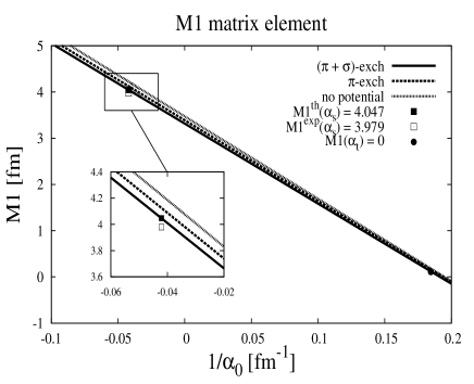
Figure 5: The matrix element ${\cal M}(\gamma,\alpha)$ for $\gamma=\gamma_{d}$ as a function of the inverse scattering length $\alpha_{0}$. This function should fulfill the properties ${\cal M}(\gamma_{d},\alpha_{s})={\cal M}_{M1}$ (the neutron capture M1 matrix element) and ${\cal M}(\gamma_{d},\alpha_{t})=0$ (the orthogonality relation between the deuteron and the zero energy triplet state. The experimental values are highlighted as points.

V Symmetry breaking

V.1 Symmetry breaking with two counter-terms

An essential ingredient of the present analysis is the requirement of orthogonality between different energy states, which ultimately reflects the self-adjoint character of the Hamiltonian. This implies that, for the Yukawa like potentials we are dealing with, the only way to parameterize the unknown information at short distances is by allowing, besides the regular solution, the irregular one and fixing the appropriate combination by imposing a value of the scattering length as an independent renormalization condition. This may appear too restrictive and in fact it is possible to renormalize using energy dependent boundary conditions, a procedure essentially equivalent to imposing more renormalization conditions or counter-terms. Although there are subtleties on how short distances should be parameterized in such way that the cut-off may be removed Pavon Valderrama and Arriola (2007); Entem et al. (2008) the procedure in coordinate space turns out to be rather simple. In the case of two conditions we would fix the scattering length, $\alpha_{0}$, and the effective range $r_{0}$ independently of the potential. The coordinate space procedure Pavon Valderrama and Arriola (2007); Entem et al. (2008) consists of expanding the wave function in powers of the energy

$$u_{p}(r)=u_{0}(r)+p^{2}u_{2}(r)+\dots\,,$$ (44)

where $u_{0}(r)$ and $u_{2}(r)$ satisfy the following equations,

$$-u_{0}^{\prime\prime}(r)+MV(r)u_{0}(r) = 0\,,$$ (45)

$$u_{0}(r) \to 1-r/\alpha_{0}\,,$$

$$-u_{2}^{\prime\prime}(r)+MV(r)u_{2}(r) = u_{0}(r)\,,$$ (46)

$$u_{2}(r) \to \left(r^{3}-3\alpha_{0}r^{2}+3\alpha_{0}r_{0}r\right)/(6\alpha_{0})\,,$$

The asymptotic conditions correspond to fix $\alpha_{0}$ and $r_{0}$ as independent parameters (two counter-terms). The matching condition at the boundary $r=r_{c}$ becomes energy dependent Pavon Valderrama and Arriola (2007)

$$\frac{u^{\prime}_{p}(r_{c})}{u_{p}(r_{c})}=\frac{u^{\prime}_{0}(r_{c})+p^{2}u^{\prime}_{2}(r_{c})+\dots}{u_{0}(r_{c})+p^{2}u_{2}(r_{c})+\dots}\,.$$ (47)

whence the corresponding phase shift may be deduced by integrating in Eq. (45) and Eq. (46) and integrating out the finite energy equation. It is worth mentioning that the energy dependent matching condition, Eq. (47), is quite unique since this is the only representation guaranteeing the existence of the limit $r_{c}\to 0$ for singular potentials Pavon Valderrama and Arriola (2007). In any case, if $r_{0}$ is fixed from the start to their experimental values in the singlet and triplet channels, the Wigner correlation given by Eq. (32) and generating the universal curve shown in Fig. 1 would not be predicted and the symmetry between the ${}^{1}S_{0}$ and the ${}^{3}S_{1}$ channels would be further hidden into the phase shifts. Note that the breaking of the symmetry with two counter-terms is a short distance one when the cut-off is eliminated, $r_{c}\to 0$, since at any rate the potential is kept fixed and $V_{s}(r)=V_{t}(r)$ for any non-vanishing distance, $r\geq r_{c}>0$. Thus, if we write

$$r_{0}=A+\frac{B}{\alpha_{0}}+\frac{C}{\alpha_{0}^{2}}+r_{0}^{\rm short}\,,$$ (48)

with $r_{0}^{\rm short}$ the effect of the second counter-term, we would obtain

$$r_{t}-r_{s}\sim r_{t}^{\rm short}-r_{s}^{\rm short}+B\left[\frac{1}{\alpha_{t}}-\frac{1}{\alpha_{s}}\right]+\dots$$ (49)

where small $1/\alpha^{2}$ terms have been neglected. This yields $r_{t}^{\rm short}-r_{s}^{\rm short}\sim 0.1{\rm fm}$. Thus, while introducing no counter-term (trivial boundary condition) does not break the symmetry yielding identical phase shifts, $\delta_{s}(k)=\delta_{t}(k)$, introducing more than one counter-term (energy dependent boundary condition) breaks the symmetry at the $\sim 10\%$ level. As a consequence, we stick to the case of just one counter-term (energy independent boundary condition).

V.2 Symmetry breaking due to the tensor force

Of course, an interesting possibility which should be explored further is that of keeping the energy independence of the boundary condition and breaking the symmetry by introducing a long distance component of the potential, such as e.g. the tensor force, which would include the coupling of the ${}^{3}S_{1}$ wave treated here to the ${}^{3}D_{1}$ channel. Actually, this would correspond to take into account, as proposed in Ref. Kaplan and Manohar (1997), the leading and complete large-$N_{c}$ NN potential. In other words, while Wigner symmetry implies a vanishing tensor force, leading large-$N_{c}$ does not necessarily implies the tensor force to be small. To analyze this potential source of conflict we consider the ${}^{3}S_{1}$ effective range parameter which incorporates a D-wave contribution stemming from S-D tensor force mixing and is given by

$$r_{t} = 2\int_{0}^{\infty}\left[\left(1-\frac{r}{\alpha_{t}}\right)^{2}-u_{0,\alpha}(r)^{2}-w_{0,\alpha}(r)^{2}\right]dr\,.$$

where the zero energy S-wave function $u_{0,\alpha}(r)\to u_{0,^{3}S_{1}}(r)$ (discussed above) and the D-wave function $w_{0,\alpha}(r)\to 0$ when the tensor force is switched off keeping $\alpha_{t}$ fixed. The corresponding tensor potential would include $\pi$ and $\rho$ exchange contributions characterized by the $g_{\pi NN}$ and $f_{\rho NN}$ couplings and diverges as $1/r^{3}$ at short distances. This situation resembles a previous OPE study Pavon Valderrama and Ruiz Arriola (2005) and a detailed account will be presented elsewhere Calle Cordón and Ruiz Arriola (2008). There, it will be shown how the extension of the superposition principle and renormalization to the coupled channel case yields in fact an identical analytical result as shown in Eq. (32) for the triplet (un-coupled) channel in the absence of tensor force. We will just quote here the numerical modification of the correlation relation coefficients for the triplet channel (the singlet ${}^{1}S_{0}$ is not modified), Eq. (32). Numerically, we get for $f_{\rho NN}=17$ and $g_{\omega NN}=9.86$

$$r_{t} = 2.6199-\frac{5.7843}{\alpha_{t}}+\frac{5.7608}{\alpha_{t}^{2}}\,.$$ (51)

which corresponds to a $\sim 10\%$ breaking due to the tensor force. As we see, the coefficients in Eq. (33) are not modified much despite the singularity of the tensor force and its dominance at short distances. Actually, the dependence of the coefficients on the couplings responsible for the tensor force is moderate in a wide range. Therefore, while from the large $N_{c}$ viewpoint a large tensor force is not forbidden, we find the effect in the S-wave to be numerically small, as implied by Wigner symmetry.

In this regard it should be noted that a virtue of the renormalization approach is that, since the scattering lengths are always fixed, such a long distance symmetry breaking term only influences the region where the potential is resolved, and from this viewpoint the perturbation will be stable, i.e. the change will be small. Actually, in Ref. Pavon Valderrama and Ruiz Arriola (2005) a suitable form of perturbation theory in the tensor force was suggested based on the known smallness of the mixing angle $\epsilon_{1}$, which stays below $2-3^{o}$, in a wide energy range and is indeed smaller than the $\delta_{\beta}$ phase. It would be interesting to work out the consequences of such an approach when also $\rho$ exchange is incorporated.

V.3 Symmetry breaking in non-central waves

With the previous appealing interpretation of the Wigner symmetry as a long distance one for the S-waves, we analyze what are the consequences for the phase shifts corresponding to partial waves at angular momentum larger than zero, $L>0$. Unlike the S-waves we expect the dependence on the short distance behavior to be suppressed due to the centrifugal barrier, and the symmetry should become more evident. Note also that while a dissimilarity between phase shifts connected by the symmetry does not necessarily imply long distance symmetry breaking, an identity between phase shifts is a clear hint of the symmetry.

In the two-nucleon system the Wigner symmetry implies the following relations for spin-isospin components of the antisymmetric sextet, ${\bf 6}_{A}$, and the symmetric decuplet, ${\bf 10}_{S}$, respectively (see Appendix A) thus we should have

$$\delta_{LJ}^{01} = \delta_{LJ}^{10}=\delta_{L}\,,\qquad{\rm even}-L$$ (52)

$$\delta_{LJ}^{00} = \delta_{LJ}^{11}=\delta_{L}\,,\qquad{\rm odd}\,-L$$ (53)

For P-waves, for instance, we have the spin singlet state ${}^{1}P_{1}$ and the spin triplets ${}^{3}P_{0}$,${}^{3}P_{1}$ and ${}^{3}P_{2}$ which according to the symmetry should be degenerate as they belong to the ${\bf 10}_{S}$ supermultiplet. Inspection of the Nijmegen analysis Stoks et al. (1993) reveals that ${}^{1}P_{1}$ is very similar to ${}^{3}P_{1}$ at all energies, $|\delta_{{}^{1}P_{1}}-\delta_{{}^{3}P_{1}}|\sim 1^{0}$, but very different from the ${}^{3}P_{0}$ and ${}^{3}P_{2}$ phases. For D-waves, associated to a ${\bf 6}_{A}$ supermultiplet, we have a similarity between ${}^{1}D_{2}$ and ${}^{3}D_{3}$ phases $|\delta_{{}^{1}D_{2}}-\delta_{{}^{3}D_{3}}|\sim 1^{0}$ but, again, clear differences between the ${}^{3}D_{1}$ and ${}^{3}D_{2}$ ones. Clearly, the symmetry is broken in higher partial waves. In what follows we want to determine whether our interpretation of a long distance symmetry which worked so successfully for S-waves above (see Sect. IV) holds also for non-central phases.

As it is well-known the spin-orbit interaction lifts the independence on the total angular momentum, via the operator $\vec{L}\cdot\vec{S}$. Moreover, the tensor coupling operator, $S_{12}$, mixes states with different orbital angular momentum. We proceed in first order perturbation theory, by using the Wigner symmetric distorted waves as the unperturbed states. In appendix D we show this procedure explicitly. To first order in spin-orbit and tensor force perturbation the following sum rule for the center of the $S=1$ multiplet, denoted by $\delta_{L}^{10}$ and $\delta_{L}^{11}$, and the $S=0$ states, denoted as $\delta_{L}^{01}$ and $\delta_{L}^{00}$, holds,

$$\delta_{L}^{10} \equiv \frac{\sum_{J=L-1}^{L+1}(2J+1)\delta_{LJ}^{10}}{(2L+1)3}=\delta_{LL}^{01}\equiv\delta_{L}^{01}\,,$$

$$\delta_{LL}^{11} \equiv \frac{\sum_{J=L-1}^{L+1}(2J+1)\delta_{LJ}^{11}}{(2L+1)3}=\delta_{LL}^{00}\equiv\delta_{L}^{00}\,,$$ (54)

In terms of these mean phases, Wigner symmetry is formulated for non-central waves as

$$\ \delta_{{}^{1}P_{1}} = \frac{1}{9}\left(\delta_{{}^{3}P_{0}}+3\delta_{{}^{3}P_{1}}+5\delta_{{}^{3}P_{2}}\right)$$ (55)

$$\delta_{{}^{1}D_{2}} = \frac{1}{15}\left(3\delta_{{}^{3}D_{1}}+5\delta_{{}^{3}D_{2}}+7\delta_{{}^{3}D_{3}}\right)$$ (56)

$$\delta_{{}^{1}F_{3}} = \frac{1}{21}\left(5\delta_{{}^{3}F_{2}}+7\delta_{{}^{3}F_{3}}+9\delta_{{}^{3}F_{4}}\right)$$ (57)

$$\delta_{{}^{1}G_{4}} = \frac{1}{27}\left(7\delta_{{}^{3}G_{3}}+9\delta_{{}^{3}G_{4}}+11\delta_{{}^{3}G_{5}}\right)\,.$$ (58)

Figure 6: Average values of the phase shifts Stoks et al. (1993) (in degrees) as a function of the CM momentum (in MeV) based on first order spin-orbit coupling. (Upper left panel) P-waves. (Upper right panel) D-waves. (Lower left panel) F-waves. (Lower right panel) G-waves. According to the Wigner symmetry $\delta_{{}^{1}L}=\delta_{{}^{3}L}$. Serber symmetry implies $\delta_{{}^{3}L}=0$ for odd-L. One sees that L-even waves satisfy Wigner symmetry while L-odd waves satisfy Serber symmetry.

These sum rules are true as long as the short distance breaking can be considered small, and for this reason we have not written down the sum rule for S-waves. Further, they hold also when the tensor force is added. In Fig. 6 we show the l.h.s. and the r.h.s. of P-, D-, F- and G-waves. As we see the D-waves fulfill this relation rather accurately up to $p\sim 250{\rm MeV}$ and the G-waves up to $p\sim 400{\rm MeV}$ while the P- and F-waves fail completely. Actually, at threshold, $\delta_{L}\to-\alpha_{L}p^{2L+1}$, and using the low energy parameters of the NijmII and Reid93 potentials Stoks et al. (1993) determined in Ref. Pavon Valderrama and Arriola (2005) we get

$$\alpha_{{}^{1}P_{1}} = \frac{1}{9}\left(\alpha_{{}^{3}P_{0}}+3\alpha_{{}^{3}P_{1}}+5\alpha_{{}^{3}P_{2}}\right)\,,$$

$$(-2.46{\rm fm}^{3}) (0.08{\rm fm}^{3})\,,$$

$$\alpha_{{}^{1}D_{2}} = \frac{1}{15}\left(3\alpha_{{}^{3}D_{1}}+5\alpha_{{}^{3}D_{2}}+7\alpha_{{}^{3}D_{3}}\right)\,,$$

$$(-1.38{\rm fm}^{5}) (-1.23{\rm fm}^{3})\,,$$ (59)

where the numerical values are displayed below the sum rules. On the light of the previous discussions for the S-waves one reason for the discrepancy should be looked in a short distance breaking of the symmetry for the D-waves. Actually, the fact that D-waves violate the sum rule at $p\sim 250{\rm MeV}$ while the G-waves show no violation up to $p\sim 400{\rm MeV}$ agrees with our interpretation in the S-waves that the Wigner symmetry be a long distance one, since higher partial waves are less sensitive to short distance effects. The case of P-waves is different since the ${}^{1}P$-potential and the ${}^{3}P$-potentials are very different. This pattern of symmetry breaking agrees with the findings of Ref. Kaplan and Manohar (1997) based on the large $N_{c}$ expansion where the central potential preserves the symmetry in $L$-even partial waves while it breaks the symmetry in the $L$-odd partial waves, since at leading order and neglecting the tensor force

$$V(r)=V_{C}(r)+\sigma\tau W_{S}(r)+{\cal O}(1/N_{c})\,,$$ (60)

so that for the lower L-channels we have

$$V_{{}^{1}S}=V_{{}^{3}S}\,, = V_{C}(r)-3W_{S}(r)+{\cal O}(1/N_{c})\,,$$

$$V_{{}^{1}P} = V_{C}(r)+9W_{S}(r)+{\cal O}(1/N_{c})\,,$$

$$V_{{}^{3}P} = V_{C}(r)+W_{S}(r)+{\cal O}(1/N_{c})\,,$$

$$V_{{}^{1}D}=V_{{}^{3}D} = V_{C}(r)-3W_{S}(r)+{\cal O}(1/N_{c})\,,$$

so as we see $V_{{}^{3}P}\neq V_{{}^{1}P}$, and thus it is obvious that $\delta_{{}^{3}P}\neq\delta_{{}^{1}P}$. One might check this further by proceeding as follows. In the case of odd waves such as the P-waves the proper comparison might be taking the ${}^{3}P$-potential and renormalizing with the ${}^{3}P$-mean scattering length, $\alpha_{{}^{3}P}=0.08{\rm fm}^{3}$ and compare to the ${}^{3}P$-mean phase shift.

We note that the initial claim of Ref. Kaplan and Savage (1996) on the validity of the Wigner symmetry based on the large $N_{c}$ expansion was restricted to purely center potentials, which do not faithfully distinguish the two irreducible representations, ${\bf 10}_{S}$ and ${\bf 6}_{A}$, of the $SU(4)$ group for the NN system. Later on, the issue was qualified by a more complete study carried out in Ref. Kaplan and Manohar (1997) which in fact could not justify the Wigner symmetry in odd-L partial waves, even when the tensor force was neglected. Although this appeared as a puzzling result, it is amazing to note that our calculations clearly show that the pattern of $SU(4)$-symmetry breaking supports a weak violation in even-L partial waves and a strong violation in the odd-L partial waves, exactly as the large $N_{c}$ expansion suggests.

V.4 Serber symmetry

On the other hand, from the odd-waves we see from Fig. 6 that the mean triplet phase is close to null, thus one might attribute this feature to an accidental symmetry where the odd-waves potentials are likewise negligible. In the large $N_{c}$ limit this means $V_{C}+W_{S}\gg V_{C}+9W_{S}$, a fact which is well verified. For instance at short distances the Yukawa OBE potentials have Coulomb like behavior $V\to C/(4\pi r)$ with the dimensionless combinations

$$C_{V_{C}+W_{S}} = -g_{\sigma NN}^{2}+g_{\omega NN}^{2}+\frac{f_{\rho NN}^{2}m_{\rho}^{2}}{6M_{N}^{2}}$$

$$C_{V_{C}+9W_{S}} = -g_{\sigma NN}^{2}+g_{\omega NN}^{2}+\frac{3f_{\rho NN}^{2}m_{\rho}^{2}}{2M_{N}^{2}}$$

where the small OPE contribution has been dropped. Numerically we get $C_{V_{C}+W_{S}}\sim 10$ and $C_{V_{C}+9W_{S}}\sim 300$ for reasonable choice of couplings. Although this approximate vanishing of triplet odd-wave potentials is not a consequence of large $N_{c}$ it is nevertheless reminiscent of the old and well-known Serber force,

$$V_{\rm Serber}(r) = \frac{1}{2}\left(1+P_{M}\right)\frac{1}{2}\left(1-P_{\sigma}\right)V_{s}(r)$$ (63)

$$+ \frac{1}{2}\left(1-P_{M}\right)\frac{1}{2}\left(1+P_{\sigma}\right)V_{t}(r)\,,$$

with $P_{M}$ the Majorana coordinate exchange operator. Due to the Pauli principle $P_{M}P_{\sigma}P_{\tau}=-1$ with $P_{\tau}=(1+\tau)/2$ and $P_{\sigma}=(1+\sigma)/2$ the isospin and spin exchange yields vanishing potentials for spin-triplet and isospin-triplet channels, and generating a scattering amplitude which is even in the CM scattering angle, a property which is approximately well fulfilled experimentally for pp-scattering. We call this property Serber symmetry for definiteness. After introducing spin-orbit coupling we would get the sum rules to first order

$$\delta_{{}^{3}P} \equiv \frac{1}{9}\left(\delta_{{}^{3}P_{0}}+3\delta_{{}^{3}P_{1}}+5\delta_{{}^{3}P_{2}}\right)=0\,,$$ (64)

$$\delta_{{}^{3}F} \equiv \frac{1}{21}\left(5\delta_{{}^{3}F_{2}}+7\delta_{{}^{3}F_{3}}+9\delta_{{}^{3}F_{4}}\right)=0\,,$$ (65)

which is well fulfilled by the phase shifts Stoks et al. (1993) as shown in Fig. 6 where $\delta_{{}^{3}P}\ll\delta_{{}^{1}P}$ and $\delta_{{}^{3}F}\ll\delta_{{}^{1}F}$. In the large $N_{c}$ limit we may comply both with Wigner symmetry in L-even waves and Serber symmetry in L-odd waves when $W_{S}(r)=-V_{C}(r)$, whence generally $V(r)=V_{C}(r)(1-\sigma\tau)$. Even if we neglect the small OPE effects, this will clearly not be exactly fulfilled unless one would require $m_{\rho}=m_{\omega}=m_{\sigma}$. Although there are schemes where such an identity between scalar and vector meson masses are explicitly verified Weinberg (1990); Svec (1997); Megias et al. (2004), at present, it is unclear whether the Serber symmetry which we observe in the NN system for spin-triplet and odd-L phase-shifts could be formulated as a symmetry from the underlying QCD Lagrangean.

Our findings suggest that a pure large $N_{c}$ in the absence of tensor force not only is compatible with the standard Wigner symmetry in the case of the dominant S-waves and higher L-even channels, but it might also be a competitive alternative for the L-odd waves where the usual Wigner symmetry is broken and Serber symmetry holds instead. Of course it would be interesting to pursue the more complete situation including the tensor force from the start, a case which will be presented elsewhere Calle Cordón and Ruiz Arriola (2008).

V.5 NN Level density in the continuum

Our results have some impact for hot nuclear matter at low densities. In the continuum, we may think of putting the two nucleon system in a box and evaluate the corresponding level density when the infinite volume limit is taken. This is a standard problem in statistical mechanics which appears, e.g. in the calculation of the second virial coefficient contribution to the equation of state of a dilute quantum gas Dashen et al. (1969) (see Refs. Horowitz and Schwenk (2006); Mallik et al. (2008) for recent applications to hot nuclear matter). The result is expressed as

$$\rho(E)=\frac{1}{2\pi i}{\rm Tr}\left[S(E)^{\dagger}\frac{dS(E)}{dE}\right]=\frac{1}{\pi}\frac{d\Delta_{NN}(E)}{dE}\,,$$ (66)

where $S(E)$ is the S matrix in all coupled channels and the total phase $\Delta$ is defined by

$$\Delta_{NN}(E)=\sum_{S,T,J}(2J+1)(2T+1)\delta_{LJ}^{ST}(E)\,.$$ (67)

In the case of coupled channels one should consider the corresponding eigenphases . Defining the mean phase as

$$\delta_{L}^{ST}(E)\equiv\frac{\sum_{J=L-S}^{L+S}(2J+1)\delta_{LJ}^{ST}(E)}{(2S+1)(2L+1)}\,,$$ (68)

corresponding to the phase-shift analog of the center of gravity of the supermultiplet (see also Eq. (54) we get

$$\Delta_{NN}(E)=\sum_{S,T,J}(2S+1)(2L+1)(2T+1)\delta_{L}^{ST}(E)\,.$$ (69)

Thus, using the above relations, Eq. (58) for L-even waves and Eq. (65) for L-odd waves, featuring Wigner and Serber symmetries respectively we would get that mixed triplet channel contributions may be either eliminated in terms of singlet ones for even-L or do not contribute for odd-L,

$$\Delta_{NN}(E)=3\left(\delta_{{}^{1}S_{0}}+\delta_{{}^{3}S_{1}}\right)+3\delta_{{}^{1}P_{1}}+30\delta_{{}^{1}D_{2}}+\dots$$ (70)

For the neutron case we have

$$\Delta_{nn}(E)=\delta_{{}^{1}S_{0}}+5\delta_{{}^{1}D_{2}}+9\delta_{{}^{1}G_{4}}+\dots$$ (71)

i.e., odd-L waves do not contribute. The lack of a P-wave contribution scaling as $\sim-\alpha_{P}p^{3}$ is compatible with the minimum observed in Ref. Horowitz and Schwenk (2006) for $\Delta_{nn}$ in the subthreshold region $E_{\rm LAB}<50{\rm MeV}$.

VI Conclusions

At low energies NN interactions are dominated by two S-waves in different channels where spin-isospin $(S,T)$ are interchanged, $(1,0)\leftrightarrow(0,1)$. Wigner $SU(4)$ symmetry implies that the potentials in the ${}^{1}S_{0}$ and ${}^{3}S_{1}$ channels coincide and the tensor force vanishes, while the corresponding phase shifts from Partial Wave Analyses are actually very different at all energies and show no evident trace of the identity of the potential, besides the qualitative fact that a weakly bound deuteron ${}^{3}S_{1}$ state and an almost bound virtual ${}^{1}S_{0}$ take place. Given the fact that the nuclear force at short distances is fairly unknown, the validity of the symmetry to all distances would be at least questionable and could hardly be tested quantitatively. On the other hand, our lack of knowledge of the short distance physics should not be crucial at low energies, where the phase shifts are indeed quite dissimilar. Therefore, we propose to regard $SU(4)$ as a long distance symmetry which might be strongly broken at short distances and weakly broken at large distances. Using renormalization ideas where the desirable short distance insensitivity is manifestly fulfilled we have shown how the standard Wigner correlation between potentials indeed predicts one phase shift from the other in a non-trivial and successful way. Remarkably, using a large $N_{c}$ motivated One Boson Exchange potential we have proven that if one channel is described successfully the other channel is unavoidably well reproduced within uncertainties which might be compatible with the disregard of the tensor force and the $1/N_{c}^{2}$ corrections to the potential. This long distance correlation holds also for the virtual singlet state and the deuteron bound state. Actually, the effects of symmetry breaking at long and short distances have been analyzed and the extension to higher partial waves has also been discussed, where a relation for phase shifts has been deduced. Our calculations provide a justification on the use of Wigner symmetry in light nuclei solely on the basis of the NN-interaction and suggest that a specific interpretation of the Wigner symmetry as a long distance one in conjunction with renormalization theory extends beyond the scaling region to a much wider range than assumed hitherto. It would be interesting to see how these ideas could be further exploited beyond the simple two nucleon system. However, a key question has always been what is the origin of the accidental Wigner symmetry from the underlying fundamental QCD Lagrangean and, moreover, under what conditions this is expected to be a useful symmetry. We find the large $N_{c}$ expansion in the absence of tensor force besides being compatible with the standard Wigner symmetry in the case of the low energy dominant S-waves and subdominant higher $L$-even partial waves it may also become a competitive alternative for the other $L$-odd partial waves where the usual Wigner symmetry is manifestly broken. These conclusions are remarkable, for they suggest that a unforeseen handle on the nature, applicability and interpretation of a widely used approximate nuclear symmetry may be based on a QCD distinct pattern such as the large $N_{c}$ limit. Obviously, it would be very interesting to pursue further the study of the complete large $N_{c}$ potential with inclusion of the tensor force to verify this issue in more detail Calle Cordón and Ruiz Arriola (2008). In our view this would definitely provide useful insights into QCD inspired approximation schemes in nuclear physics.

Appendix A Wigner symmetry for NN

Wigner $SU(4)$ spin-isospin symmetry consists of the following 15-generators  Wigner and Feenberg (1941); Wilkinson (1969); Van Isacker (1999)

$$T^{a} = \frac{1}{2}\sum_{A}\tau_{A}^{a}\,,$$ (72)

$$S^{i} = \frac{1}{2}\sum_{A}\sigma_{A}^{i}\,,$$ (73)

$$G^{ia} = \frac{1}{2}\sum_{A}\sigma_{A}^{i}\tau_{A}^{a}\,,$$ (74)

where $\tau_{A}^{a}$ and $\sigma_{A}^{i}$ are isospin and spin Pauli matrices for nucleon $A$ respectively, and $T^{a}$ is the total isospin, $S^{i}$ the total spin and $G^{ia}$ the Gamow-Teller transition operator. The quadratic Casimir operator reads

$$C_{SU(4)} = T^{a}T_{a}+S^{i}S_{i}+G^{ia}G_{ia}\,,$$ (75)

and a complete set of commuting operators can be taken to be $C_{SU(4)}$, $T_{3}$ and $S_{z},G_{z3}$. The fundamental representation has $C_{SU(4)}=4$ and corresponds to a single nucleon state with a quartet of states $p\uparrow$, $p\downarrow$, $n\uparrow$, $n\downarrow$, with total spin $S=1/2$ and isospin $T=1/2$ represented ${\bf 4}=(S,T)=(1/2,1/2)$. For two nucleon states with good spin $S$ and good isospin $T$ Pauli principle requires $(-)^{S+T+L}=-1$ with $L$ the angular momentum, thus

$$C_{SU(4)}^{ST}=\frac{1}{2}\left(\sigma+\tau+\sigma\tau\right)+\frac{15}{2}\,,$$ (76)

where $\tau=\tau_{1}\cdot\tau_{2}=2T(T+1)-3$ and $\sigma=\sigma_{1}\cdot\sigma_{2}=2S(S+1)-3$ and the corresponding wave function is of the form

$$\Psi(\vec{x})=\frac{u_{L}^{LS}(r)}{r}Y_{LM_{L}}(\hat{x})\chi^{SM_{S}}\chi^{TM_{T}}\,.$$ (77)

One has two supermultiplets, which Casimir values are

$$C_{SU(4)}^{00} = C_{SU(4)}^{11}=9\,,$$ (78)

$$C_{SU(4)}^{01} = C_{SU(4)}^{10}=5\,,$$ (79)

corresponding to an antisymmetric sextet ${\bf 6}_{A}=(0,1)\oplus(1,0)$ when $L=$ even and a symmetric decuplet ${\bf 10}_{S}=(0,0)\oplus(1,1)$ when $L=$odd. The radial wave functions fulfill $u_{L}^{01}(r)=u_{L}^{10}(r)$ and $u_{L}^{00}(r)=u_{L}^{11}(r)$ respectively. This means that we have the following supermultiplets

$$(^{1}S_{0},^{3}S_{1})\,,\,(^{1}P_{1},^{3}P_{0,1,2})\,,\,(^{1}D_{2},^{3}D_{1,2,3})\dots$$ (80)

When applied to the NN potential, the requirement of Wigner symmetry for all states, implies

$$V_{T} = W_{T}=V_{LS}=W_{LS}=0\,,$$

$$W_{S} = V_{S}=W_{C}\,,$$ (81)

so that the potential may be written as

$$V=V_{C}+(2C_{SU(4)}^{ST}-15)W_{S}\,.$$ (82)

Note that the particular choice $W_{S}=0$ corresponds to a spin-isospin independent potential, but in this case no distinction between the ${\bf 6}_{A}$ and ${\bf 10}_{S}$ supermultiplets arises. As it is well-known the spin-orbit interaction lifts the total angular momentum independence. The Wigner symmetry does not distinguish between different total angular momentum values, so admitting that the potentials are different we may define a common potential

$$V_{LST}(r)\equiv\frac{\sum_{J=L-S}^{L+S}(2J+1)V_{JST}(r)}{(2S+1)(2L+1)}\,,$$ (83)

where similarly to the perturbation theory for energy levels where the center of a multiplet of states is predicted, the appropriate statistical weights related to the angular momentum have been used. The previous expression makes sense if the symmetry is broken linearly by spin-orbit coupling. In terms of these mean potentials the symmetry would be

$$V_{{}^{1}L}(r)=V_{{}^{3}L}(r)\,,$$ (84)

or equivalently

$$V_{{}^{1}J_{J}}(r)=\frac{\sum_{J=L-1}^{L+1}(2J+1)V_{{}^{3}L_{J}}(r)}{3(2L+1)}\,.$$ (85)

As mentioned in the paper, if the symmetry is taken literally at all distances we should have $\delta_{{}^{1}L}=\delta_{{}^{3}L}$.

Appendix B Long distance Perturbation theory

We illustrate here a situation where the potential may be treated in long distance perturbation theory and renormalized (for a somewhat similar approach for finite cut-offs see e.g. Ref. Cohen and Hansen (1998)). Unlike the standard perturbative approach, which usually does not hold in the presence of bound states, this expansion can deal with weakly bound states, provided this is the only one. This is in fact the case for the OPE potential for the parameters we use, applied to the deuteron state, for which we show the procedure here to first order. To analyze this situation we vary the potential $V\to V+\Delta V$

$$-\Delta u_{k}(r)^{\prime\prime} + M\Delta V(r)u_{k}(r)$$ (86)

$$+ MV(r)\Delta u_{k}(r)=k^{2}\Delta u_{k}(r)\,,$$

we use the previous wave functions $u_{k}(r)$ as the zeroth order approximation, corresponding to take $V(r)=0$ and solve for the first order correction $\Delta u_{k}(r)$ the equation which asymptotic wave function corresponds to take the phase shift $\delta+\Delta\delta$. Multiplying Eq. (5) by $\Delta u_{k}(r)$ and Eq. (86) by $u_{k}(r)$, subtracting both equations and integrating from $r_{c}$ to $\infty$ we get

$$\left[-u_{k}^{\prime}\Delta u_{k}+u_{k}\Delta u_{k}\right]\Big{|}_{r_{c}}^{\infty}=\int_{r_{c}}^{\infty}dr\,\Delta U(r)u_{k}(r)^{2}\,.$$ (87)

The lower limit term may be related to the variation of the boundary condition, whereas the upper limit term is related to the change in the phase shift, $\Delta\delta$. In order to eliminate the cut-off we subtract the zero energy limit, $k\to 0$, and using the energy independence of the boundary condition we get some cancellation since

$$\Delta\left(\frac{u_{k}^{\prime}(r_{c})}{u_{k}(r_{c})}-\frac{u_{0}^{\prime}(r_{c})}{u_{0}(r_{c})}\right)=0\,.$$ (88)

Finally, the result may be re-written as follows

$$\Delta\left(k\cot\delta\right) = -\Delta\left(\frac{1}{\alpha_{0}}\right)$$

$$+ \int_{r_{c}}^{\infty}\Delta U(r)\left[u_{k}(r)^{2}-u_{0}(r)^{2}\right]dr\,.$$

If we fix the scattering length independently on the potential we have $\Delta\alpha_{0}=0$, thus eliminating the first term of the r.h.s. and after taking the limit $r_{c}\to 0$ the result for the total (and renormalized) phase shift to first order in the potential reads

$$k\cot\delta_{0}(k) = -\frac{1}{\alpha_{0}}+\int_{0}^{\infty}dr\,MV(r)$$

$$\times \left(\left[\cos(kr)-\frac{\sin(kr)}{\alpha_{0}k}\right]^{2}-\left[1-\frac{r}{\alpha_{0}}\right]^{2}\right)+\dots$$

The renormalized effective range is entirely predicted from the potential at all distances

$$r_{0}=4\int_{0}^{\infty}drr^{2}MV(r)\left(1-\frac{r}{\alpha_{0}}\right)^{2}+\dots$$ (91)

Note the extra power suppression at the origin when $\alpha_{0}$ is fixed independently on the potential, indicating short distances become less important. The bound state can be obtained in a similar manner by replacing $u_{k}(r)\to u_{\gamma}(r)$, assuming that the binding energy is independent on the potential, $\Delta\gamma=0$, and using orthogonality Eq. (88) to the zero energy state

$$\frac{1}{\alpha_{0}}=\gamma+\int_{0}^{\infty}MV(r)\left[u_{\gamma}(r)^{2}-u_{0}(r)^{2}\right]dr\,.$$ (92)

This equation is implicit in both $\alpha_{0}$ and $\gamma$, but we can make it perturbative explicitly, using that to first order $\alpha_{0}\sim 1/\gamma$ in the zero energy wave function $u_{0}(r)\sim 1-\gamma r$, yielding

$$\frac{1}{\alpha_{0}}=\gamma+\int_{0}^{\infty}MV(r)\left[e^{-2\gamma r}-(1-\gamma r)^{2}\right]dr$$ (93)

Appendix C Scale invariance and renormalization

We have suggested that Wigner symmetry be a long distance one. From a renormalization group (RG) viewpoint this has a simple interpretation (for a discussion in coordinate space see e.g. Ref. Pavon Valderrama and Ruiz Arriola (2004); Pavon Valderrama and Arriola (2007)). It means finding a solution to the RG equations which break the symmetry of the equations. A very simple case which illustrates this issue is provided by the problem

$$-u^{\prime\prime}(r)+\frac{g}{r^{2}}u(r)=k^{2}u(r)\,.$$ (94)

At zero energy, $k=0$, the solution is invariant under the scaling transformation $r\to\lambda r$. This property holds also at short distances, where the energy term on the r.h.s. can be neglected. If we use the RG equation, Eq. (35), for this particular case at short distances

$$Rc_{0}^{\prime}(R)=c_{0}(R)(1-c_{0}(R))+g\,.$$ (95)

The scale symmetry becomes now evident; if $c_{0}(R)$ is a solution then $c_{0}(\lambda R)$ is also a solution for any value of $\lambda\neq 0$. The solution must necessarily specify the value at a given scale $c_{0}(R_{0})$, hence breaking explicitly the dilatation symmetry. This symmetry breaking is unavoidable. In Refs. Pavon Valderrama and Ruiz Arriola (2004); Pavon Valderrama and Arriola (2007) it is shown how, for $g<-1/4$ the breaking is lowered to the discrete subgroup of dilatations, and the connection to the Russian Doll renormalization. In the case of the Wigner symmetry for the ${}^{1}S_{0}$ and ${}^{3}S_{0}$ potentials discussed in the paper, the breaking is not unavoidable, and there exists in fact a very special choice where the symmetry can be preserved by taking identical boundary conditions at a given scale. Besides this particular solution, the identity between solutions $c_{0,s}(R)$ and $c_{0,t}(R)$ will generally be violated, although the relation from one scale to a different one $c_{0,s}(R_{0})\to c_{0,s}(R)$ and $c_{0,t}(R_{0})\to c_{0,t}(R)$ is governed by the same relation, Eq. (35).

It is worth noting the resemblance of the previous quantum-mechanical discussion with similar and well-known field theoretical concepts. The unavoidable breaking of the dilatation symmetry corresponds to an anomaly of the dilatation current. The optional choice of boundary conditions corresponds to the case of finite but ambiguous theories (see e.g. Ref. Jackiw (2000)).

Appendix D Splitting formula for phase-shifts

We want to derive the splitting formula for phase shifts, Eq. (54) by using distorted waves perturbation theory. The coupled channel Schrödinger equation for the relative motion reads

$$-{\bf u}^{\prime\prime}(r)+\left[{\bf U}(r)+\frac{{\bf L}^{2}}{r^{2}}\right]{\bf u}(r)=k^{2}{\bf u}(r)\,,$$ (96)

where ${\bf U}^{SJ}_{L,L^{\prime}}(r)=2\mu_{np}{\bf V}^{SJ}_{L,L^{\prime}}(r)$ is the coupled channel matrix potential which for the total angular momentum $J>0$ can be written as,

$${\bf U}^{0J}(r) = U_{JJ}^{0J}$$

$${\bf U}^{1J}(r) = \left(\begin{matrix}U_{J-1,J-1}^{1J}(r)&0&U_{J-1,J+1}^{1J}(r)\cr 0&U_{JJ}^{1J}(r)&0\cr U_{J-1,J+1}^{1J}(r)&0&U_{J+1,J+1}^{1J}(r)\end{matrix}\right)\,$$

In Eq. (96) ${\bf L}^{2}={\rm diag}(L_{1}(L_{1}+1),\dots,L_{N}(L_{N}+1))$ is the angular momentum, ${\bf u}(r)$ is the reduced matrix wave function and $k$ the C.M. momentum. In the case at hand $N=1$ for the spin singlet channel with $L=J$ and $N=3$ for the spin triplet channel with $L_{1}=J-1$, $L_{2}=J$ and $L_{3}=J+1$. For ease of notation we will keep the compact matrix notation of Eq. (96). At long distances, we assume the asymptotic normalization condition

$${\bf u}(r)\to\hat{\bf h}^{(-)}(r)-\hat{\bf h}^{(+)}(r){\bf S}\,,$$ (98)

with ${\bf S}$ the standard coupled channel unitary S-matrix. For the spin singlet state, $S=0$, one has $L=J$ and hence the state is un-coupled

$$S_{JJ}^{0J}=e^{2i\delta_{J}^{0J}}\,,$$ (99)

whereas for the spin triplet state $S=1$, one has the un-coupled $L=J$ state

$$S_{JJ}^{1J} = e^{2i\delta_{J}^{1J}}\;,$$ (100)

and the two channel coupled states $L,L^{\prime}=j\pm 1$ states which written in terms of the eigenphases are

$$S^{1J} = \left(\begin{matrix}\cos\epsilon_{J}&-\sin\epsilon_{J}\cr\sin\epsilon_{J}&\cos\epsilon_{J}\end{matrix}\right)\left(\begin{matrix}e^{2{\rm i}\delta^{1J}_{J-1}}&0\cr 0&e^{2{\rm i}\delta_{J+1}^{1J}}\end{matrix}\right)$$ (101)

$$\times \left(\begin{matrix}\cos\epsilon_{J}&\sin\epsilon_{J}\cr-\sin\epsilon_{J}&\cos\epsilon_{J}\end{matrix}\right)\,.$$

The corresponding out-going and in-going free spherical waves are given by

$$\hat{\bf h}^{(\pm)}(r) = {\rm diag}(\hat{h}^{\pm}_{L_{1}}(kr),\dots,\hat{h}^{\pm}_{L_{N}}(kr))\,,$$ (102)

with $\hat{h}^{\pm}_{L}(x)$ the reduced Hankel functions of order $l$, $\hat{h}_{L}^{\pm}(x)=xH_{L+1/2}^{\pm}(x)$ ( $\hat{h}_{0}^{\pm}=e^{\pm ix}$ ), and satisfy the free Schrödinger’s equation for a free particle.

In order to determine the infinitesimal change of the $S$ matrix, ${\bf S}\to{\bf S}+\Delta{\bf S}$, under a general deformation of the potential ${\bf U}(r)\to{\bf U}(r)+\Delta{\bf U}(r)$ we use Schrödinger’s equation (96) and the standard Lagrange’s identity adapted to this particular case, we get

$$\left[{\bf u}(r)^{\dagger}\Delta{\bf u}^{\prime}(r)-{\bf u}^{\prime}(r)^{\dagger}\Delta{\bf u}(r)\right]^{\prime}={\bf u}(r)^{\dagger}\Delta{\bf U}(r){\bf u}(r)\,.$$

The unitarity of the S-matrix, ${\bf S}^{\dagger}{\bf S}={\bf 1}$, yields the condition $\Delta{\bf S}^{\dagger}{\bf S}+{\bf S}^{\dagger}\Delta{\bf S}=0$. We assume a mixed boundary condition at short distances, $r=r_{c}$, for the unperturbed coupled channel potential, ${\bf U}(r)$,

$${\bf u}^{\prime}(r_{c})+{\bf L}{\bf u}(r_{c})=0\,,$$ (104)

with ${\bf L}$ a self-adjoint matrix. After integration from the cut-off radius $r_{c}$ to infinity and using the asymptotic form of the matrix wave function, Eq. (98), as well as the condition at the origin, Eq. (104) yields

$$2{\rm i}k{\bf S}^{\dagger}\Delta{\bf S}=\int_{r_{c}}^{\infty}dr\,{\bf u}(r)^{\dagger}\Delta{\bf U}(r){\bf u}(r)\,.$$ (105)

If we take the Wigner symmetric states as the unperturbed problem, then ${\bf S}$ , ${\bf U}(r)$ and ${\bf u}(r)$ become a diagonal matrices, so that

$$\Delta\delta_{JL}^{ST}=-\frac{1}{2p}\int_{r_{c}}^{\infty}dr\,u_{L}^{ST}(r)^{\dagger}\Delta{\bf U}(r)u_{L}^{ST}(r)\,,$$ (106)

so that the perturbed eigenphases become

$$\delta_{JL}^{ST}=\delta_{L}^{ST}+\Delta\delta_{JL}^{ST}$$ (107)

Note that to this order the mixing phases vanish, $\Delta\epsilon_{J}=0$. Identifying further $\Delta{\bf U}$ with the spin-orbit and the tensor potential, in the LS-coupling the result may be written as

$$\delta_{LJ}^{ST} = \delta_{L}^{ST}+\delta_{S,1}C_{L}^{ST}(S_{12}^{J})_{LL}$$

$$+ A_{L}^{ST}\left[J(J+1)-L(L+1)-S(S+1)\right]\,,$$

where $(S_{12}^{J})_{J-1,J-1}=-2(J-1)/(2J+1)$, $(S_{12}^{J})_{J,J}=2$, $(S_{12}^{J})_{J+1,J+1}=-2(J+2)/(2J+1)$. Defining the supermultiplet coefficients $A_{L}=A_{L}^{10}=A_{L}^{01}$ and $B_{L}=A_{L}^{00}=A_{L}^{11}$

$$\delta_{LJ}^{10} = \delta_{LJ}^{01}+A_{L}\left[J(J+1)-L(L+1)-2\right]$$ (109)

$$+ C_{L}(S_{12}^{J})_{LL}\,,$$

$$\delta_{LJ}^{11} = \delta_{LJ}^{00}+B_{L}\left[J(J+1)-L(L+1)-2\right]$$ (110)

$$+ D_{L}(S_{12}^{J})_{LL}\,,$$

we readily get the sum rule for phase-shifts, Eq. (54). The above equations would yield a Lande-like interval rule between spin-triplet energy levels for the spin-orbit or the tensor potentials separately. For instance,

$$\delta_{{}^{1}P_{1}} = \delta_{P}\,,$$

$$\delta_{{}^{3}P_{0}} = \delta_{P}-4D_{1}-4B_{1}\,,$$

$$\delta_{{}^{3}P_{1}} = \delta_{P}+2D_{1}-2B_{1}\,,$$

$$\delta_{{}^{3}P_{2}} = \delta_{P}-\frac{2}{5}D_{1}+2B_{1}\,.$$ (111)

A further remark is in order, since the spin-orbit or tensor potentials may be singular at the origin. In such a case of singular perturbations one computes the sum rule first and then removes the cut-off, $r_{c}\to 0$.

References

- Van Isacker (1999) P. Van Isacker, Reports of Progress in Physics 62, 1661 (1999).
- Wigner and Feenberg (1941) E. P. Wigner and E. Feenberg, Reports of Progress in Physics 8, 274 (1941).
- Wilkinson (1969) D. H. E. Wilkinson, Isospin in Nuclear Physics (New York ;John Wiley and Sons, Inc. (1969)., 1969).
- Wigner (1937) E. Wigner, Phys. Rev. 51, 106 (1937).
- Hund (1937) F. Hund, Zeitschrift fur Physik 105, 202 (1937).
- Donnelly and Walker (1970) T. W. Donnelly and G. E. Walker, Annals of Physics 60, 209 (1970).
- Cauvin et al. (1981) M. Cauvin, V. Gillet, F. Soulmagnon, and M. Danos, Nucl. Phys. A361, 192 (1981).
- Van Isacker et al. (1997) P. Van Isacker, O. Juillet, and B. K. Gjelsten, Found. Phys. 27, 1047 (1997).
- Vogel and Ormand (1993) P. Vogel and W. E. Ormand, Phys. Rev. C47, 623 (1993).
- Nayak and Kota (2001) R. C. Nayak and V. K. B. Kota, Phys. Rev. C64, 057303 (2001).
- Van Isacker et al. (1995) P. Van Isacker, D. D. Warner, and D. S. Brenner, Phys. Rev. Lett. 74, 4607 (1995).
- Chen et al. (2004) J.-W. Chen, D. Lee, and T. Schafer, Phys. Rev. Lett. 93, 242302 (2004), eprint nucl-th/0408043.
- ’t Hooft (1974) G. ’t Hooft, Nucl. Phys. B72, 461 (1974).
- Witten (1979) E. Witten, Nucl. Phys. B160, 57 (1979).
- Kaplan and Savage (1996) D. B. Kaplan and M. J. Savage, Phys. Lett. B365, 244 (1996), eprint hep-ph/9509371.
- Kaplan and Manohar (1997) D. B. Kaplan and A. V. Manohar, Phys. Rev. C56, 76 (1997), eprint nucl-th/9612021.
- Machleidt et al. (1987) R. Machleidt, K. Holinde, and C. Elster, Phys. Rept. 149, 1 (1987).
- Banerjee et al. (2002) M. K. Banerjee, T. D. Cohen, and B. A. Gelman, Phys. Rev. C65, 034011 (2002), eprint hep-ph/0109274.
- Belitsky and Cohen (2002) A. V. Belitsky and T. D. Cohen, Phys. Rev. C65, 064008 (2002), eprint hep-ph/0202153.
- Cohen (2002) T. D. Cohen, Phys. Rev. C66, 064003 (2002), eprint nucl-th/0209072.
- Riska (2002) D. O. Riska, Nucl. Phys. A710, 55 (2002), eprint nucl-th/0204016.
- Mehen et al. (1999) T. Mehen, I. W. Stewart, and M. B. Wise, Phys. Rev. Lett. 83, 931 (1999), eprint hep-ph/9902370.
- Epelbaum et al. (2002) E. Epelbaum, U. G. Meissner, W. Gloeckle, and C. Elster, Phys. Rev. C65, 044001 (2002), eprint nucl-th/0106007.
- Epelbaum et al. (2003) E. Epelbaum, U.-G. Meissner, and W. Gloeckle, Nucl. Phys. A714, 535 (2003), eprint nucl-th/0207089.
- Beane and Savage (2003) S. R. Beane and M. J. Savage, Nucl. Phys. A717, 91 (2003), eprint nucl-th/0208021.
- Braaten and Hammer (2003) E. Braaten and H. W. Hammer, Phys. Rev. Lett. 91, 102002 (2003), eprint nucl-th/0303038.
- Epelbaum et al. (2006) E. Epelbaum, H. W. Hammer, U.-G. Meissner, and A. Nogga, Eur. Phys. J. C48, 169 (2006), eprint hep-ph/0602225.
- Hammer et al. (2007) H. W. Hammer, D. R. Phillips, and L. Platter, Eur. Phys. J. A32, 335 (2007), eprint 0704.3726.
- Beane et al. (2006) S. R. Beane, P. F. Bedaque, K. Orginos, and M. J. Savage, Phys. Rev. Lett. 97, 012001 (2006), eprint hep-lat/0602010.
- Ishii et al. (2007) N. Ishii, S. Aoki, and T. Hatsuda, Phys. Rev. Lett. 99, 022001 (2007), eprint nucl-th/0611096.
- Aoki et al. (2008) S. Aoki, T. Hatsuda, and N. Ishii (2008), eprint 0805.2462.
- Stoks et al. (1993) V. G. J. Stoks, R. A. M. Kompl, M. C. M. Rentmeester, and J. J. de Swart, Phys. Rev. C48, 792 (1993).
- Pavon Valderrama and Arriola (2006) M. Pavon Valderrama and E. R. Arriola, Phys. Rev. C74, 054001 (2006), eprint nucl-th/0506047.
- Pavon Valderrama and Arriola (2007) M. Pavon Valderrama and E. R. Arriola (2007), eprint 0705.2952.
- Partovi and Lomon (1970) M. H. Partovi and E. L. Lomon, Phys. Rev. D2, 1999 (1970).
- Stoks et al. (1994) V. G. J. Stoks, R. A. M. Klomp, C. P. F. Terheggen, and J. J. de Swart, Phys. Rev. C49, 2950 (1994), eprint nucl-th/9406039.
- Machleidt (2001) R. Machleidt, Phys. Rev. C63, 024001 (2001), eprint nucl-th/0006014.
- Ruiz Arriola et al. (2007) E. Ruiz Arriola, A. Calle Cordon, and M. Pavon Valderrama (2007), eprint 0710.2770.
- Calle Cordon and Ruiz Arriola (2008) A. Calle Cordon and E. Ruiz Arriola (2008), eprint 0804.2350.
- Jackiw (2000) R. Jackiw, Int. J. Mod. Phys. B14, 2011 (2000), eprint hep-th/9903044.
- Entem et al. (2008) D. R. Entem, E. Ruiz Arriola, M. Pavon Valderrama, and R. Machleidt, Phys. Rev. C77, 044006 (2008), eprint 0709.2770.
- Valderrama et al. (2008) M. P. Valderrama, A. Nogga, E. Ruiz Arriola, and D. R. Phillips, Eur. Phys. J. A36, 315 (2008), eprint 0711.4785.
- Caprini et al. (2006) I. Caprini, G. Colangelo, and H. Leutwyler, Phys. Rev. Lett. 96, 132001 (2006), eprint hep-ph/0512364.
- Pavon Valderrama and Ruiz Arriola (2004) M. Pavon Valderrama and E. Ruiz Arriola, Phys. Rev. C70, 044006 (2004), eprint nucl-th/0405057.
- Birse et al. (1999) M. C. Birse, J. A. McGovern, and K. G. Richardson, Phys. Lett. B464, 169 (1999), eprint hep-ph/9807302.
- Pavon Valderrama and Ruiz Arriola (2005) M. Pavon Valderrama and E. Ruiz Arriola, Phys. Rev. C72, 054002 (2005), eprint nucl-th/0504067.
- Calle Cordón and Ruiz Arriola (2008) A. Calle Cordón and E. Ruiz Arriola (2008), eprint In preparation.
- Pavon Valderrama and Arriola (2005) M. Pavon Valderrama and E. R. Arriola, Phys. Rev. C72, 044007 (2005).
- Weinberg (1990) S. Weinberg, Phys. Rev. Lett. 65, 1177 (1990).
- Svec (1997) M. Svec, Phys. Rev. D55, 5727 (1997), eprint hep-ph/9607297.
- Megias et al. (2004) E. Megias, E. Ruiz Arriola, L. L. Salcedo, and W. Broniowski, Phys. Rev. D70, 034031 (2004), eprint hep-ph/0403139.
- Dashen et al. (1969) R. Dashen, S.-K. Ma, and H. J. Bernstein, Phys. Rev. 187, 345 (1969).
- Horowitz and Schwenk (2006) C. J. Horowitz and A. Schwenk, Nucl. Phys. A776, 55 (2006), eprint nucl-th/0507033.
- Mallik et al. (2008) S. Mallik, J. N. De, S. K. Samaddar, and S. Sarkar, Phys. Rev. C77, 032201 (2008), eprint 0801.0498.
- Cohen and Hansen (1998) T. D. Cohen and J. M. Hansen, Phys. Lett. B440, 233 (1998), eprint nucl-th/9808006.