Abstract

MEMS storage devices are new non-volatile secondary storages that have outstanding advantages over magnetic disks. MEMS storage devices, however, are much different from magnetic disks in the structure and access characteristics. They have thousands of heads called probe tips and provide the following two major access facilities: (1) flexibility : freely selecting a set of probe tips for accessing data, (2) parallelism : simultaneously reading and writing data with the set of probe tips selected. Due to these characteristics, it is nontrivial to find data placements that fully utilize the capability of MEMS storage devices. In this paper, we propose a simple logical model called the Region-Sector (RS) model that abstracts major characteristics affecting data retrieval performance, such as flexibility and parallelism, from the physical MEMS storage model. We also suggest heuristic data placement strategies based on the RS model and derive new data placements for relational data and two-dimensional spatial data by using those strategies. Experimental results show that the proposed data placements improve the data retrieval performance by up to 4.0 times for relational data and by up to 4.8 times for two-dimensional spatial data of approximately 320 Mbytes compared with those of existing data placements. Further, these improvements are expected to be more marked as the database size grows.

1 Introduction

Micro-Electro-Mechanical Systems (MEMS) is a technology that integrates electronic circuits and mechanical parts into one chip [20]. MEMS storage devices are new non-volatile secondary storages based on the MEMS technology. The prototypes of MEMS storage devices have been developed by Carnegie Mellon University (CMU), IBM laboratory, and Hewlett-Packard laboratory. Recently, there have been a number of efforts to increase its capacity and to improve the performance [9].

MEMS storage devices have outstanding advantages compared with magnetic disks: average access time is ten times faster, average bandwidth is thirteen times larger, and power consumption is 54 times lower; their size is as small as $1cm^{2}$ [17]. Due to these advantages, MEMS storage devices are expected to be widely used in many places, such as the secondary storage of a laptop [7] and the middle-level storage to reduce the performance gap between main memory and disk in the memory hierarchy [16, 23].

MEMS storage devices, however, are much different from magnetic disks in the structure and access characteristics. They have thousands of heads called probe tips to access data. MEMS storage devices also have the following two major access characteristics [18]: (1) flexibility : freely selecting a set of probe tips for accessing data, (2) parallelism : simultaneously reading and writing data with the set of probe tips selected. For good data retrieval performance, it is necessary to place data on MEMS storage devices taking advantage of their structures and access characteristics [6, 18, 21, 22, 23].

There have been a number of studies on data placement for MEMS storage devices. In the operating systems field, methods have been proposed that abstract the MEMS storage device as a linear array of fixed-size logical blocks with one head [4, 6]. These methods allow us to use the MEMS storage device easily just like a disk, but provide relatively poor data retrieval performance because they do not take full advantage of the characteristics of MEMS storage devices [18]. In the database field, methods have been proposed to directly place data on the MEMS storage device based on data access patterns of applications [21, 22]. These methods provide relatively good data retrieval performance [18], but are quite sophisticated because they directly manage MEMS storage devices having a complicated structure.

In this paper, we propose a logical model called the Region-Sector (RS) model that abstracts the physical MEMS storage model. The RS model abstracts major characteristics affecting data retrieval performance – flexibility and parallelism – from the physical MEMS storage model. The RS model is simple enough for users to easily understand and use the MEMS storage device and, at the same time, is strong enough to provide capability comparable to that of a physical MEMS storage model. We also suggest heuristic data placement strategies based on the RS model. These strategies allow us to find data placements efficiently for a given application.

The contributions of this paper are as follows: (1) we propose the RS model, which is a logical abstraction of the MEMS storage device; (2) we suggest heuristic data placement strategies based on the RS model; (3) we derive new data placements for relational data and two-dimensional spatial data by using those strategies; (4) through extensive analysis and experiments, we show that the data retrieval performances of our data placements are superior or comparable to those of existing data placements.

The rest of this paper is organized as follows. Section 2 introduces the MEMS storage device. Section 3 describes prior art related to data placement for the MEMS storage device. Section 4 proposes the RS model. Section 5 presents heuristic data placement strategies. Section 6 presents new data placements derived by using heuristic data placement strategies. Section 7 presents the results of performance evaluation. Section 8 summarizes and concludes the paper.

2 MEMS Storage Devices

The MEMS storage device is composed of a media sled and a probe tip array. Figure 1 shows the structure of the MEMS storage device. The media sled is a square plate on which data is read and written by recording techniques such as magnetic, thermomechanical, and phase-change ones [18]. The media sled has $R_{x}\times R_{y}$ squares called regions. Here, $R_{x}$ ($R_{y}$) is the number of regions in the X (Y) axis. Each region contains $S_{x}\times S_{y}$ tip sectors, which are the smallest unit of accessing data. Here, $S_{x}$ ($S_{y}$) is the number of tip sectors in a region in the X (Y) axis. A column is a set of tip sectors that have the same position in the X axis of each region [6]. The probe tip array is a set of $R_{x}\times R_{y}$ heads called probe tips. Each probe tip reads and writes data on the corresponding region of the media sled.

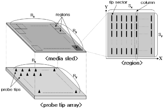
Figure 1: The structure of the MEMS storage device.

The MEMS storage device reads and writes data by moving the media sled on the probe tip array. Here, a number of probe tips can be activated so as to simultaneously read and write data. Each activated probe tip reads or writes data on the tip sector having the same relative position in each region. Users are able to freely select a set of probe tips to be simultaneously activated, the number of which is restricted to $200\sim 2,000$ due to the limitation in power consumption and electric heat [7].

The major access characteristics [18] of the MEMS storage device are summarized as follows.

Flexibility:

freely selecting and activating a set of probe tips for accessing data.

Parallelism:

simultaneously reading and writing data with the set of probe tips selected.

The MEMS storage device reads or writes data by performing the following three steps [6].

1. Activating step:

activating a set of probe tips to use  (the activating time is negligible compared with seek or transfer times).

2. Seeking step:

moving the media sled so that the probe tip is located on the target tip sector (the seek time is dependent on the distance that the media sled moves).

3. Transferring step:

reading or writing data on tip sectors that are contiguously arranged within columns while moving the media sled in the + (or -) direction of the Y axis (the transfer time is proportional to the size of data accessed).

If tip sectors to be accessed are not contiguous within a column but scattered over many columns, data are accessed by performing the steps 2 and 3 repeatedly.

We explain the seek process in more detail since it is quite different from that of the disk. The seek time can be computed using Equations (1)$\sim$(3). Let $SeekTime_{x}$ be the time to seek in the direction of the X axis, and $SeekTime_{y}$ in the direction of the Y axis. In $SeekTime_{x}$, if the media sled moves in the direction of the X axis, we have to wait until the vibration of the media sled stops. The time to wait for such vibration to stop is called the settle time. Thus, $SeekTime_{x}$ is the sum of the move time and the settle time as in Equation (1). In $SeekTime_{y}$, if the media sled moves in the opposite direction of the current direction, the media sled has to turn around. The time to turn around is called the turnaround time. Thus, $SeekTime_{y}$ is the sum of the move time and the turnaround time as in Equation (2). If the media sled moves in the same direction of the current direction, the turnaround time is zero. Since the media sled is capable of moving in the direction of both the X axis and the Y axis simultaneously, the total seek time is the maximum of $SeekTime_{x}$ and $SeekTime_{y}$ as in Equation (3).

$$SeekTime_{x} = MoveTime_{x}~{}~{}~{}+~{}~{}~{}SettleTime$$ (1)

$$SeekTime_{y} = MoveTime_{y}~{}~{}~{}+~{}~{}~{}TurnaroundTime$$ (2)

$$SeekTime = MAX~{}(~{}SeekTime_{x}\,,~{}~{}SeekTime_{y}~{})$$ (3)

Table 1 summarizes the parameters and values of the CMU MEMS storage device being widely used for research [2, 6]. We use them in this paper. In Table 1, $T_{X}$ ($T_{Y}$) is the average time to move from one random position to another in the direction of the X (Y) axis [2].

Table 1: The parameters and values of the CMU MEMS storage device.

Symbols	Definitions	Values
$R_{x}$	the number of regions in the direction of the X axis	80
$R_{y}$	the number of regions in the direction of the Y axis	80
$N_{R}$	the number of regions (= $R_{x}\times R_{y}$)	$6,400$
$S_{x}$	the number of tip sectors in a region in the direction of the X axis	2500
$S_{y}$	the number of tip sectors in a region in the direction of the Y axis	27
$N_{S}$	the number of tip sectors in a region (= $S_{x}\times S_{y}$)	$67,500$
$N_{PT}$	the number of probe tips	6,400
$N_{APT}$	the maximum number of active probe tips	1,280
$SectorSize$	the size of data area in a tip sector (bits)	64
$TransferRate$	the transfer rate per probe tip (Mbit/s)	0.7
$T_{X}$	the average move time in the direction of the X axis (ms)	0.52
$T_{Y}$	the average move time in the direction of the Y axis (ms)	0.35
$T_{S}$	the average settle time (ms)	0.215
$T_{T}$	the average turnaround time (ms)	0.06

3 Related Work

There have been a number of studies on data placement for the MEMS storage device. We classify them into two categories – disk mapping approaches and device-specific approaches – depending on whether they take advantage of the characteristics of the storage device. This classification of the MEMS storage device is analogous to that of the flash memory [5], which is another type of new non-volatile secondary storage. For the flash memory, device-specific approaches (e.g., Yet Another Flash File System (YAFFS) [12]) provide new mechanisms to exploit the features of the flash memory in order to improve performance, while disk mapping approaches(e.g., Flash Translation Layer (FTL) [1]) abstract the flash memory as a linear array of fixed-size pages in order to use existing disk-based algorithms on the flash memory. In this section, we explain two categories for the MEMS storage device in more detail.

3.1 Disk Mapping Approaches

Griffin et al. [6] and Dramaliev et al. [4] proposed models to use the MEMS storage device just like a disk. They abstract the MEMS storage device as a linear array of fixed-size logical blocks with one head. This linear abstraction works well for most applications using the MEMS storage device as the replacement of the disk [6]. However, they provide relatively poor data retrieval performance compared with device-specific approaches [21, 22] because they do not take full advantage of the characteristics of the MEMS storage device [18].

3.2 Device-specific Approaches

Yu et al. [21, 22] proposed methods for placing data on the MEMS storage device based on data access patterns of applications. Yu et al. [22] places relational data on the MEMS storage device such that projection queries are performed efficiently. Yu et al. [21] places two-dimensional spatial data such that spatial range queries are performed efficiently. These data placements identify that data access patterns of such applications are inherently two-dimensional, and then, place data so as to take advantage of parallelism and flexibility of the MEMS storage device. We explain each data placement in more detail for comparing them with our methods in Section 6.

3.2.1 Data Placement for Relational Data

Yu et al. [22] deals with the application that places a relation on the MEMS storage device, and then, executes simple projection queries over that relation. Here, queries read the values of the specified attributes of all tuples. Figure 2 shows an example relation $R$, which has $k$ attributes $attr_{1},...,attr_{k}$ and has $n$ tuples. Here, $a_{i,j}$ represents the $j$ th attribute value of the $i$ th tuple ($1\leq i\leq n$, $1\leq j\leq k$).

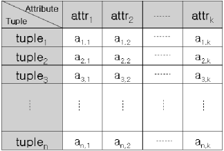
Figure 2: An example relation $R$.

Figure 3 shows Yu et al. [22]’s data placement of the relation $R$ on the MEMS storage device. Here, for simplicity of explanation, we assume that the length of each attribute value is equal to the size of the tip sector. First, a set of $m$ tuples ($tuple_{1}\sim tuple_{m}$) is placed on the first tip sector of each region, i.e., the shaded tip sectors in Figure 3. Likewise, each set of $m$ tuples ($tuple_{m\times(i-1)+1}\sim tuple_{m\times i}$) is placed on the $i$ th tip sector of the region ($2\leq i\leq\lceil\frac{n}{m}\rceil$) in the column-prime order. Equation (10) shows a mapping function $f_{RelationtoMEMS}$ that puts the attribute value $a_{v,w}$ into the tip sector $<$$r_{x},r_{y},s_{x},s_{y}$$>$ of the MEMS storage device.

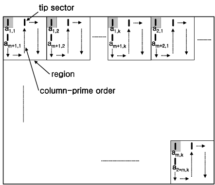
Figure 3: Yu et al.’s data placement.

$$f_{RelationtoMEMS}\,(a_{v,w})=\left\{\begin{array}[]{l}r_{x}=((k\times((v-1)~{}\mathtt{mod}~{}m)+w)-1)~{}\mathtt{mod}~{}R_{x}+1\\ r_{y}=\lceil\frac{(k\times((v-1)\,\mathtt{mod}\,m)+w)}{R_{x}}\rceil\\ s_{x}=\lceil\frac{\lceil\frac{v}{m}\rceil}{S_{y}}\rceil\\ s_{y}=\left\{\begin{array}[]{ll}(\lceil\frac{v}{m}\rceil-1)~{}\mathtt{mod}~{}S_{y}+1&\mbox{if $s_{x}$ is odd}\\ S_{y}-((\lceil\frac{v}{m}\rceil-1)~{}\mathtt{mod}~{}S_{y})&\mbox{if $s_{x}$ is even}\end{array}\right.\end{array}\right.$$ (10)

3.2.2 Data Placement for Two-dimensional Spatial Data

Yu et al. [21] deals with an application that places a set of two-dimensional spatial objects on the MEMS storage device, and then, executes region queries over those objects. Here, the two-dimensional spatial objects are uniformly distributed in the two-dimensional space, and queries read objects contained in a rectangular region. Figure 4 shows an example set $S$ of two-dimensional $N_{PT}\times N_{PT}$ spatial objects.

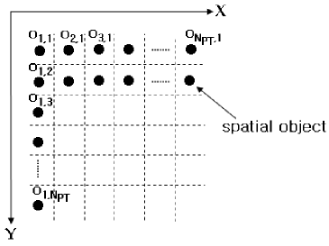
Figure 4: An example set $S$ of two-dimensional spatial objects.

Figure 5 shows Yu et al. [21]’s data placement of the set $S$ in the MEMS storage device. Here, for simplicity of explanation, we assume that each object is stored in one tip sector. In Figure 5, the objects from $o_{1,1}$ to $o_{N_{PT},1}$ are first placed on the first tip sector of each region. Likewise, the objects from $o_{1,i}$ to $o_{N_{PT},i}$ on the $i$ th tip sector of each region ($2\leq i\leq 6400$) in the column-prime order. Equation (17) shows a mapping function $f_{SpacetoMEMS}$ that places the object $o_{x,y}$ on the tip sector $<$$r_{x},r_{y},s_{x},s_{y}$$>$ of the MEMS storage device.

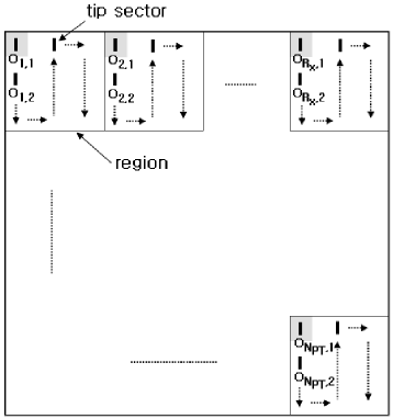
Figure 5: Yu et al.’s data placement.

$$f_{SpacetoMEMS}\,(o_{x,y})=\left\{\begin{array}[]{l}r_{x}=(x-1)~{}\mathtt{mod}~{}N_{R_{x}}+1\\ r_{y}=\lceil\frac{x}{N_{R_{x}}}\rceil\\ s_{x}=\lceil\frac{y}{N_{S_{y}}}\rceil\\ s_{y}=\left\{\begin{array}[]{ll}(y-1)~{}\mathtt{mod}~{}N_{S_{y}}+1&\mbox{if $s_{x}$ is odd}\\ N_{S_{y}}-((y-1)~{}\mathtt{mod}~{}N_{S_{y}})&\mbox{if $s_{x}$ is even}\end{array}\right.\end{array}\right.$$ (17)

4 Region-Sector (RS) Model for the MEMS Storage Device

In this Section, we propose the RS model for the MEMS storage device. In Section 4.1, we provide an overview of the RS model. In Section 4.2, we formally define the RS model. In Section 4.3, we present the mapping function between the RS model and the MEMS storage device.

4.1 Overview

The RS model can be regarded as a virtual view of the physical MEMS storage device. The purpose of the model is to provide an abstraction making it easy to understand and simple to use the complex MEMS storage device while maintaining its performance and flexibility.

When placing data on the disk, the OS and applications abstract the disk as a relatively simple logical view such as a linear array of fixed-sized logical blocks because considering the physical structures (cylinders, tracks, and sectors) of the disk is complex. This kind of abstraction can also be applied to the MEMS storage device. By abstracting the MEMS storage device as a relatively simple logical view such as the RS model, we can more easily place data on the MEMS storage device than when we directly consider the physical structures (regions, columns, tip sectors).

Figure 6 shows three kinds of system architectures for using the MEMS storage device. Figure 6(a) shows one using the disk-based algorithms and the disk mapping layer (explained in Section 3.1); Figure 6(b) one using the MEMS storage device-specific algorithms (explained in Section 3.2) without any mapping layer; and Figure 6(c) one using the RS model-specific algorithms and the RS model layer. The architecture in Figure 6(c) is capable of providing higher performance compared with that in Figure 6(a) by taking advantage of useful characteristics of the MEMS storage device through the RS model. It also helps us find good data placements for a given application more easily than the architecture in Figure 6(b) because it hides complex features of the physical MEMS storage device.

                           

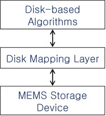
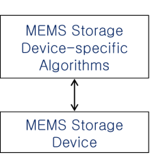
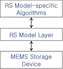
(a) The disk mapping layer           (b) The device-specific algorithm         (c) The RS model layer

architecture.                                architecture.                                architecture.

Figure 6: The architectures of the system for the MEMS storage device.

4.2 Definition of the RS Model

The RS model maps the tip sectors of the MEMS storage device into a virtual two-dimensional plane in order to effectively use parallelism and flexibility. For the mapping, we first classify the tip sectors into two groups depending on the possibility of using parallelism. It is possible to use parallelism for the tip sectors having the same relative $(x,y)$ position in each region because we are able to freely select a set of tip sectors and simultaneously access them. Hereafter, we call the set of tip sectors having the same relative $(x,y)$ positions in each region as the simultaneous-access sector group. On the other hand, it is not possible to use parallelism for the tip sectors existing in the same region because we are able to access only one tip sector at a time from them. Hereafter, we call the set of such tip sectors as the non-simultaneous-access sector group.

Figure 7 shows the structure of the RS model. The RS model is composed of a set of probe tips and a two-dimensional plane. The set of probe tips are lined up horizontally. We call them the probe tip line. The two-dimensional plane has the Region axis and the Sector axis. The RS model maps the tip sectors in a simultaneous-access sector group in the direction of the Region axis and those in a non-simultaneous-access sector group in the direction of the Sector axis. We map the tip sectors in the non-simultaneous-access sector group (i.e., tip sectors in a region) in the column-prime order as shown in Figure 7 since it is the fastest order to access all the tip sectors in a region [17, 22]. We call an ordered set of tip sectors that have the same position in the Region axis a linearized region. The RS model regards the tip sectors within a linearized region as quasi-contiguous. Each probe tip reads and writes data on the corresponding linearized region of the RS model.

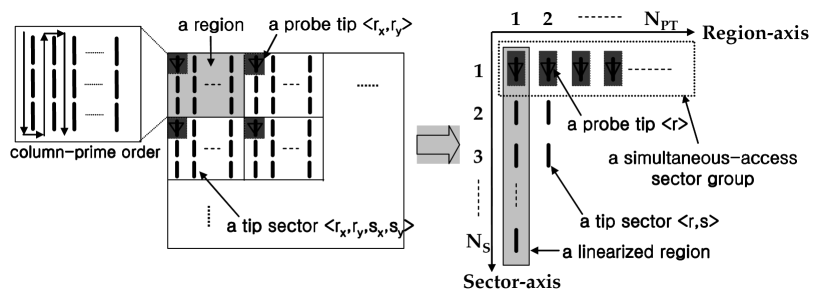
          (a) The MEMS storage device.                            (b) The Region-Sector (RS) model.

Figure 7: The structure of the RS model.

The RS model simplifies the structure of the MEMS storage device by reducing the number of parameters to represent the position of a tip sector. In the MEMS storage device, the position of a tip sector is represented by four parameters $<$$r_{x},r_{y},s_{x},s_{y}$$>$ ($1$$\leq$$r_{x}$$\leq$$R_{x}$, $1$$\leq$$r_{y}$$\leq$$R_{y}$, $1$$\leq$$s_{x}$$\leq$$S_{x}$, $1$$\leq$$s_{y}$$\leq$$S_{y}$) as shown in Figure 7(a), where $<$$r_{x},r_{y}$$>$ is the position of the region and $<$$s_{x},s_{y}$$>$ the position of the tip sector within the region. On the other hand, in the RS model, the position of a tip sector is represented by only two parameters $<$$r,s$$>$ as shown in Figure 7(b), where $r$ is the position of the tip sector in the Region axis and $s$ in the Sector axis.

The RS model reads or writes data by performing the following three steps repeatedly (as compared to the physical MEMS storage device described in Section 2).

1. Activating step:

activating a set of probe tips to use.

2. Seeking step:

moving the probe tip line to the target row.

3. Transferring step:

reading or writing data on tip sectors that are quasi-contiguously arranged within linearized regions while moving the probe tip line in the + (or -) direction of the Sector axis.

The RS model considers quasi-contiguous tip sectors within a linearized region to be sequentially accessed (the reason will be explained later), while the MEMS storage device is capable of sequentially accessing contiguous tip sectors only within a column.

We explain the seek time and transfer rate of the RS model. Through calculation using them, users can approximately estimate the data access time in the MEMS storage device exactly mapping the data to the MEMS storage device. The calculation of data access time in the RS model is easier because the movement of probe tips in the RS model is modeled simpler than that in the MEMS storage device.

For the seek time of the RS model, for simplicity, we use the average seek time of the physical MEMS storage device. By using the average seek time instead of the real seek time, we can significantly simplify the cost model for data retrieval performance while little sacrificing the accuracy of the cost model.

In the RS model, the transfer rate per probe tip is calculated as the data size of a region divided by the time to read all the tip sectors of a region in the column-prime order. We note that the RS model considers all quasi-contiguous tip sectors within a linearized region to be sequentially accessed. Table 2 summarizes some notation to be used for calculating the transfer rate.

Table 2: The notation to be used for calculating the transfer rate per probe tip in the RS model.

Symbols	Definitions
$S_{x}$	the number of columns in a region
$S_{y}$	the number of tip sectors in a column
$SectorSize$	the size of a tip sector (bytes)
$RegionSize$	the size of a region (bytes) (= $S_{x}\times S_{y}\times SectorSize$)
$TransferRate$	the transfer rate per probe tip in the physical MEMS storage device (Mbytes/s)
$SeekTime_{adj}$	the seek time from a column to an adjacent column in the physical MEMS
	storage device (s)

The transfer rate per probe tip in the RS model is computed as in Equation (18). The time to read data of a region in the column-prime order is the sum of the following two terms: (1) the time to read data of each column, (2) the time to seek to the adjacent column for each column. The former is $\frac{RegionSize}{TransferRate}$, and the latter $S_{x}\times SeekTime_{adj}$. $SeekTime_{adj}$ is computed as in Equation (19). Because the move time to the adjacent column $MoveTime_{adj\_x}$ is negligible compared with $SettleTime$, and $SettleTime$ is larger than $TurnaroundTime$, $SeekTime_{adj}$ is approximately equal to $SettleTime$.

$$TransferRate_{rs} = \frac{RegionSize}{(\,\frac{RegionSize}{TransferRate}\,)~{}~{}~{}+~{}~{}~{}(\,S_{x}\times{SeekTime_{adj}}\,)}$$ (18)

$$SeekTime_{adj} = MAX\,(\,MoveTime_{adj\_x}~{}+~{}SettleTime\,,~{}~{}TurnaroundTime\,)$$ (19)

$$\approx SettleTime$$

The characteristics of the RS model in both random and sequential accesses are not much different from those of the MEMS storage device. The seek time of the RS model is equal to that of the MEMS storage device since the RS model uses the average time to seek from one random position to another in a certain region of the MEMS storage device. In Equation (18), the total seek time (i.e., $S_{x}\times SeekTime_{adj}$) is only about 6 % of the time to read all the tip sectors of a region. Thus, the transfer rate of the RS model is approximately equal to that of the MEMS storage device.

Table 3 summarizes the differences between the RS model and the physical MEMS storage model.

Table 3: Comparison of the RS model with the physical MEMS storage model.

	MEMS storage model	RS model	Remarks
addressing the position	$<$$r_{x},r_{y},s_{x},s_{y}$$>$	$<$$r,s$$>$	simpler
of a tip sector
movement of	in the +/- direction of	in the +/- direction of	simpler
probe tips	the X and Y axes	the Sector axis
the area of	$S_{y}$ tip sectors	$N_{S}=S_{x}\times S_{y}$ tip sectors	expanded by $S_{x}$ times
sequential access	within a column	within a linearized region
		(quasi-contiguous)
seek time	real seek time	average seek time	equal in average
		from one random position
		to another
transfer rate	real transfer rate	average transfer rate	approximately equal
		when accessing tip sectors
		in a region in the
		column-prime order

4.3 Mapping Functions between the RS Model and the MEMS Storage Device

In order to use the RS model, it is necessary to map the position of each tip sector in the RS model into that in the MEMS storage model, and vice versa. In this section, we define two mapping functions $f_{RStoMEMS}$ and $f_{MEMStoRS}$. In Equation (26), $f_{RStoMEMS}$ is for converting the position $<$$r,s$$>$ in the RS model into the position $<$$r_{x},r_{y},s_{x},s_{y}$$>$ in the MEMS storage model. In Equation (31), $f_{MEMStoRS}$ is for converting the position $<$$r_{x},r_{y},s_{x},s_{y}$$>$ into the position $<$$r,s$$>$.

$$f_{RStoMEMS}\,(<r,~{}s>)=\left\{\begin{array}[]{l}r_{x}=(r-1)~{}\mathtt{mod}~{}R_{x}+1\\ r_{y}=\lfloor\frac{(r-1)}{R_{x}}\rfloor+1\\ s_{x}=\lfloor\frac{(s-1)}{S_{y}}\rfloor+1\\ s_{y}=\left\{\begin{array}[]{ll}(s-1)~{}\mathtt{mod}~{}S_{y}+1&\mbox{if $s_{x}$ is odd}\\ S_{y}-((s-1)~{}\mathtt{mod}~{}S_{y})&\mbox{if $s_{x}$ is even}\end{array}\right.\end{array}\right.$$ (26)

$$f_{MEMStoRS}\,(<r_{x},~{}r_{y},~{}s_{x},~{}s_{y}>)=\left\{\begin{array}[]{l}r=(R_{x}\times(r_{y}-1))+r_{x}\\ s=\left\{\begin{array}[]{ll}(S_{y}\times(s_{x}-1))+s_{y}&\mbox{if $s_{x}$ is odd}\\ (S_{y}\times(s_{x}-1))+(S_{y}-s_{y}+1)&\mbox{if $s_{x}$ is even}\end{array}\right.\end{array}\right.$$ (31)

In practice, two mapping functions $f_{RStoMEMS}$ and $f_{MEMStoRS}$ are implemented as a driver between user algorithms (i.e., RS model-specific algorithms in Figure 6(c)) and the MEMS storage device. If users write and execute programs that place and access data on the RS model, the data are automatically placed and accessed on the MEMS storage device by this driver.

5 Data Placement Strategies in the RS model

For secondary storage devices, data retrieval performance is significantly affected by data placement on them. The same holds for the MEMS storage device. For good data retrieval performance, we need to place data on the MEMS storage device taking advantage of its structure and access characteristics [6, 18, 21, 22, 23]. In this section, we present heuristic data placement strategies that help us efficiently find good data placements.

As the measure of data retrieval performance, we use the time to read the data being retrieved by a query as was done by Yu et al. [21, 22]. We call it the retrieval time. Table 4 summarizes the notation to be used for analyzing the retrieval time in the RS model.

Table 4: The notation to be used for analyzing the retrieval time in the RS model.

Symbols	Definitions
$RetrievalDataSize$	the size of the data being retrieved by a query (bytes)
$TransferRate_{rs}$	the average transfer rate per probe tip in the RS model (Mbytes/s)
$SeekTime_{rs}$	the average seek time in the RS model (s)
$K_{parallel}$	the average number of probe tips used during query processing
$K_{random}$	the average number of seek operations occurring during query processing

The retrieval time in the RS model can be computed as in Equation (32). It is the sum of $Total\-TransferTime$ and $TotalSeekTime$. $TotalTransfer\-Time$ is $RetrievalDataSize$ divided by the total transfer rate, which is $TransferRate_{rs}\times K_{parallel}$. $TotalSeekTime$ is $SeekTime_{rs}\times K_{random}$.

$$RetrievalTime = TotalTransferTime~{}~{}~{}+~{}~{}~{}TotalSeekTime$$ (32)

$$= (\,\frac{RetrievalDataSize}{TransferRate_{rs}\times K_{parallel}}\,)~{}~{}~{}+~{}~{}~{}(\,SeekTime_{rs}\times K_{random}\,)$$

From Equation (32), we know that $RetrievalTime$ decreases as $K_{parallel}$ gets larger and as $K_{random}$ gets smaller. Thus, for good performance, it is preferable to place data such that $K_{parallel}$ is made as large as possible (its maximum value is $N_{APT}$) and $K_{random}$ as small as possible (its minimum value is $0$). Theoretically, the data placement that makes $K_{parallel}=N_{APT}$ and, at the same time, $K_{random}=0$ is the optimal. However, it may not be feasible to find such data placements. Hence, we employ two simple heuristic data placement strategies as follows.

Strategy_Sequential:

a strategy that places the data being retrieved by a query as contiguously as possible in the direction of the Sector axis in the RS model. This strategy aims at making $K_{random}$ be as close to $0$ as possible.

Strategy_Parallel:

a strategy that places the data being retrieved by a query as widely as possible in the direction of the Region axis on the RS model. This strategy aims at making $K_{parallel}$ be as close to $N_{APT}$ as possible.

6 Applications of Data Placement Strategies

In this Section, we present data placements derived from Strategy_Sequential and Strategy_Parallel for two applications. We present data placements for relational data in Section 6.1, and data placements for two-dimensional spatial data in Section 6.2.

6.1 Data Placements for Relational Data

In this section, we deal with an application that places a relation on the MEMS storage device, and then, executes simple projection queries over that relation. This application is the same one dealt with by Yu et al. [22] as described in Section 3.2.1. We present two data placements for relational data. We name the data placement derived from Strategy_Sequential, which turns out to be identical to the placement proposed by Yu et al. [22], as Relational-Sequential-Yu, and the one derived from Strategy_Parallel as Relational-Parallel.

6.1.1 Relational-Sequential-Yu

Relational-Sequential-Yu intends to provide highly sequential reading of data by preventing seek operations in processing queries. Here, it is preferable that the values of the projected attributes are placed as contiguously as possible in the direction of the Sector axis. Accordingly, Relational-Sequential-Yu stores the tuples of the relation $R$ such that a linearized region is occupied with the values of only one attribute. Thus, these values are stored quasi-contiguously.

Figure 8 shows Relational-Sequential-Yu and the data area being retrieved by the query projecting $N_{projection}$ attributes. Let us assume that at most $m$ tuples are stored in one simultaneous-access sector group. As shown in Figure 8(a), Relational-Sequential-Yu puts $m$ tuples $tuple_{m\times(i-1)+j}$ ($1\leq j\leq m$) into the $i$ th simultaneous-access sector group ($1\leq i\leq\lceil\frac{n}{m}\rceil$). Equation (35) shows the mapping function $f_{RelationtoRS}$ that puts the attribute value $a_{v,w}$ into the tip sector $<$$r,s$$>$ in the RS model. In Figure 8(b), the shaded area indicates the tip sectors accessed by the query projecting $attr_{p}$ and $attr_{q}$. If the width of the shaded area (i.e., the number of tip sectors corresponding to $attr_{p}$ or $attr_{q}$ in a simultaneous-access sector group $=m\times N_{projection}$) is less than or equal to $N_{APT}$, only one sequential scan suffices for query processing. Otherwise, several sequential scans ($=\lceil\frac{m\times N_{projection}}{N_{APT}}\rceil$) are required. We use column-prime order among scans by activating another set of $N_{APT}$ probe tips .

                 

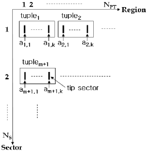
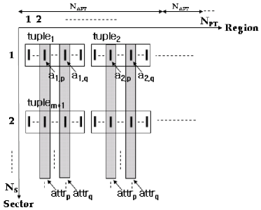
(a) Relational-Sequential-Yu.                   (b) The data area being retrieved by a query.

Figure 8: Relational-Sequential-Yu data placement and the data area being retrieved by the query projecting $attr_{p}$ and $attr_{q}$.

$$f_{RelationtoRS}\,(a_{v,w})=\left\{\begin{array}[]{l}r=k\times((v-1)~{}\mathtt{mod}~{}m)+w\\ s=\lceil\frac{v}{m}\rceil\end{array}\right.$$ (35)

Relational-Sequential-Yu is in effect identical to the data placement proposed by Yu et al. [22] in Section 3.2.1. Equation (35) is identical to the composition of Equation (31) and Equation (10), i.e., $f_{MEMStoRS}(f_{RelationtoMEMS}(a_{v,w}))$. Thus, both Relational-Sequential-Yu and Yu et al.’s data placement store the attribute value $a_{v,w}$ in the same tip sector in the MEMS storage device. Nevertheless, devising and understanding Relational-Sequential-Yu is easier than coming up with Yu et al.’s data placement since the RS model provides an abstraction of the MEMS storage device.

6.1.2 Relational-Parallel

Relational-Parallel intends to provide highly parallel reading of data by increasing the number of probe tips used during query processing. Here, it is preferable that the values of the projected attributes are placed as widely as possible in the direction of the Region axis. Accordingly, Relational-Parallel stores the values of each attribute such that a simultaneous-access sector group is occupied with the values of only one attribute.

Figure 9 shows Relational-Parallel and the data area being retrieved by the query. As shown in Figure 9(a), Relational-Parallel stores the values of an attribute $attr_{p}$  in a number of successive simultaneous-access sector groups ($1\leq p\leq k$). By such a placement, at most one seek operation occurs when reading all the values of each attribute. In Figure 9(b), the shaded area indicates the tip sectors accessed by the query projecting $attr_{p}$ and $attr_{q}$. Since the width of the shaded area is $N_{PT}$, $\lceil\frac{N_{PT}}{N_{APT}}\rceil$ sequential scans are required for each attribute .

                 

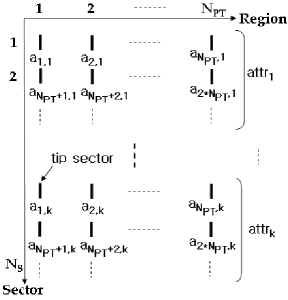
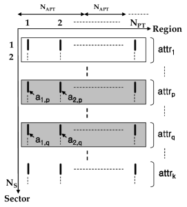
          (a) Relational-Parallel.                   (b) The data area being retrieved by the query.

Figure 9: Relational-Parallel data placement and the data area being retrieved by the query projecting $attr_{p}$ and $attr_{q}$.

In order to show the excellence of Relational-Parallel, we deal with another application that executes the range selection query in Equation (6.1.2). This was also dealt with by Yu et al. [22]

SELECT $$attr_{1},~{}~{}attr_{p},~{}~{}attr_{q},~{}~{}...$$

FROM $$R$$

WHERE $$attr_{1}~{}~{}>~{}~{}Bound;$$

Figure 10 shows the data area being retrieved by the range query. Relational-Parallel reads the values of attributes as follows: (1) for the attribute in the WHERE clause ($attr_{1}$), it reads the value of every tuple, and then, checks whether each tuple satisfies the condition $attr_{1}>Bound$; (2) for the remaining attributes in a SELECT clause ($attr_{p}$, $attr_{q}$, …, excluding $attr_{1}$), it reads only those values that belong to the tuples satisfying the condition. In Figure 10, the shaded area indicates the tip sectors accessed by the range query projecting $attr_{1}$, $attr_{p}$, and $attr_{q}$. $\lceil\frac{N_{PT}}{N_{APT}}\rceil$ sequential scans are required for the attribute $attr_{1}$; but only $\lceil\frac{N_{PT}\,\times\,query\,selectivity}{N_{APT}}\rceil$ scans are required for the attributes $attr_{p}$ and $attr_{q}$.

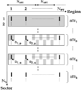
Figure 10: The data area being retrieved by the range query projecting $attr_{1}$, $attr_{p}$, and $attr_{q}$.

If relation $R$ has variable size attributes, both Relational-Sequential-Yu and Relational-Parallel consider a variable size attribute as a fixed size attribute with its maximum size as was done by Yu et al. [22].

Relational-Parallel is a new data placement that focuses on parallelism, which is an important characteristic of the MEMS storage device, while Relational-Sequential-Yu is the one that focuses on reducing the number of seek operations.

6.1.3 Comparison between Relation-Sequential-Yu and Relational-Parallel

In data placements for relational data, the parameters affecting the retrieval time are 1) the data size to be retrieved and 2) the number of attributes to be projected. In this section, we compare the retrieval time of Relational-Sequential-Yu and Relational-Parallel by using Equation (32). Table 5 summarizes the notation used for analyzing the retrieval time.

Table 5: The notation used for analyzing the retrieval time.

Symbols	Definitions
$RetrievalDataSize$	the data size to be retrieved for query processing (bytes)
$N_{projection}$	the number of attributes to be projected by a query
$m$	the number of tuples stored in one simultaneous-access sector group
	in Relational-Sequential-Yu

For $TotalSeekTime$, Relational-Sequential-Yu is better than Relational-Parallel. In Relational-Parallel, $K_{random}\leq N_{projection}$ because at most $N_{projection}$ seek operations could occur during query processing. However, in Relational-Sequential-Yu, $K_{random}=1$.

For $TotalTransferTime$, Relational-Parallel is better than Relational-Sequential-Yu. In Relational-Sequential-Yu, $K_{parallel}=min\,(m\times N_{projection},~{}N_{APT})$. On the other hand, in Relational-Parallel, since $N_{PT}$ is usually a multiple of $N_{APT}$ [6], all $N_{APT}$ probe tips are used for reading the data. Thus, $K_{parallel}=N_{APT}$.

The difference in $TotalTransferTime$ between the two data placements increases as $RetrievalData\-Size$ gets lager, while the difference in $TotlaSeekTime$ is limited to ($SeekTime_{rs}\times N_{projection}$). Thus, as $RetrievalDataSize$ exceeds a certain threshold, $RetrievalTime$ of Relational-Parallel becomes smaller than that of Relational-Sequential-Yu because the advantage in the transfer time overrides the disadvantage in the seek time.

6.1.4 Comparison with Disk-Based Data Placements

Relational-Sequential-Yu and Relational-Parallel are similar to the N-ary Storage Model (NSM) [15] and the Decomposition Storage Model(DSM) [3], respectively, which have been proposed as data placements for relational data in a disk environment. Figure 11 shows the data placements of the relational $R$ by NSM and DSM. In Figure 11(a), NSM sequentially places tuples of the relation $R$ in slotted disk pages. In Figure 11(b), DSM partitions a relation $R$ into sub-relations based on the number of attributes such that each sub-relation corresponds to an attribute. Here, DSM places an attribute value of a tuple together with the identifier of the tuple (simply, TID) so as to be used for joining sub-relations.

                 

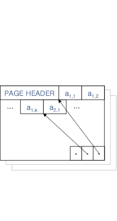
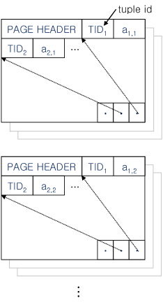
(a) NSM.                                             (b) DSM.

Figure 11: Data placements of the relation $R$ in slotted disk pages.

Although the data placements of NSM and DSM are similar to those of Relational-Sequential-Yu and Relational-Parallel, the data retrieval costs for range select queries are quite different. As mentioned in Section 3, NSM and DSM consider $N_{APT}$ probe tips as one head. But, Relational-Sequential-Yu and Relational-Parallel use multiple probe tips for accessing data by freely selecting and activating them. NSM reads all attribute values of the tuples [15, 22], while Relational-Sequential-Yu reads only the projected attribute values by using multiple probe tips. DSM reads all the values of the sub-relations corresponding to the projected attributes [3, 22], while Relational-Parallel reads only those values of the tuples that satisfy the condition by using multiple probe tips. However, if we consider the simple projection queries with no range condition, Relational-Parallel reads all the values of projected attributes as well. In this case, Relational-Parallel becomes the same as DSM.

6.2 Data Placements for Two-Dimensional Spatial Data

In this section, we deal with an application that places a set of two-dimensional spatial objects, and then, executes region queries over those objects. This application is the same one dealt with by Yu et al. [21] as described in Section 3.2.2. We consider two data placements for spatial data. We define the data placement derived by using Strategy_Sequential as Spatial-Sequential-Yu, and the one derived by using Strategy_Parallel as Spatial-Parallel. Spatial-Sequential-Yu turns out to be identical to the placement proposed by Yu et al. [21].

6.2.1 Spatial-Sequential-Yu

Spatial-Sequential-Yu intends to provide highly sequential reading of data by preventing seek operations. We place spatial objects such that a rectangular region in the two-dimensional space is represented as a rectangular region in the RS model. By such a placement, for any rectangular query region, we make $K_{random}=0$ because objects in the query region are already quasi-contiguously placed in the Sector axis of the RS model .

Figure 12 shows Spatial-Sequential-Yu. Spatial-Sequential-Yu places a spatial object in the X-Y plane on a tip sector in the Region-Sector plane. Here, we again assume that one spatial object can be stored in one tip sector. Equation (39) shows a mapping function $f_{SpacetoRS}$ that stores the object $o_{x,y}$ on the tip sector $<$$r,s$$>$ in the RS model.

          (a) The set $S$ of two-dimensional spatial objects.           (b) Placement in the RS model.

Figure 12: Spatial-Sequential-Yu.

$$f_{SpacetoRS}\,(o_{x,y})=\left\{\begin{array}[]{l}r=x\\ s=y\end{array}\right.$$ (39)

In Figure 13(a), the shaded area indicates the query region in the two-dimensional space. In Figure 13(b), the shaded area indicates the corresponding region in the RS model. Let $QueryRegionSize_{x}$ be the width of the corresponding query region. Then, $\lceil\frac{QueryRegionSize_{x}}{N_{APT}}\rceil$ sequential scans are required for query processing.

(a) The query region to be retrieved                        (b) The query region to be retrieved

in the two-dimensional space.                                        in the RS model.

Figure 13: The query region to be retrieved in Spatial-Sequential-Yu.

If the number of spatial objects in the direction of the X axis is larger than $N_{PT}$, we vertically partition the two-dimensional space into components having a width of $N_{PT}$ or less, and then, place the components on the Region-Sector plane along the direction of the Sector axis. Then, the query cost should reflect one additional seek time for each component.

Spatial-Sequential-Yu is in effect identical to the data placement proposed by Yu et al. [21] in Section 3.2.2. Equation (39) is identical to the composition of Equation (31) and Equation (17), i.e., $f_{MEMStoRS}(f_{SpacetoMEMS}(o_{x,y}))$. Thus, both Spatial-Sequential-Yu and Yu et al.’s data placement put the object $o_{x,y}$ in the same tip sector in the MEMS storage device. Nevertheless, as in Relational-Sequential-Yu, understanding Spatial-Sequential-Yu is much easier than understanding Yu et al.’s data placement due to the abstraction of the RS model.

6.2.2 Spatial-Parallel

Spatial-Parallel intends to provide highly parallel reading of data by increasing the number of probe tips used during query processing. We partition the two-dimensional space into blocks, and then, place spatial objects in a block into a simultaneous-access sector group of the RS model. By such a placement, for any rectangular query region, we can make $K_{parallel}$ to be as close to $N_{APT}$ as possible.

Figure 14 shows Spatial-Parallel, which places spatial objects through the following three steps.

1. Partitioning step:

We partition the two-dimensional space into blocks that form a rectangular grid such that the total size of spatial objects in one block is equal to the total size of tip sectors in one simultaneous sector group.

2. Ordering step:

We sort the partitioned blocks according to a space filling curve [10]. A space filling curve such as the Z-order [14] or Hilbert order [8, 13], is a way of linearly ordering regions in a multi-dimensional space into a one-dimensional space so as to keep the clustering [10]. Here, We use the Hilbert order.

3. Placement step:

We place spatial objects of the $i$ th block in the sequence constructed in Step 2 on the $i$ th simultaneous-access sector group of the RS model in the row-major order ($1\leq i\leq N_{block}$).

(a) The set $S$ of two-dimensional spatial objects.           (b) Placement in the RS model.

Figure 14: Spatial-Parallel.

Figure 15 shows the region being retrieved by a query. In Figure 15(a), the shaded area indicates the query region, and the slashed area indicates the set of blocks overlapping with the query region. Hereafter, we call this set of overlapping blocks the $QueryBlockSet$. In Figure 15(b), the shaded area indicates the corresponding query region to be retrieved in the RS model. For data retrieval, we first find the set of simultaneous-access sector groups corresponding to $QueryBlockSet$, and then, read the data on tip sectors overlapping with the query region . Here, seek operations occur at most as many times as the number of blocks in the $QueryBlockSet$.

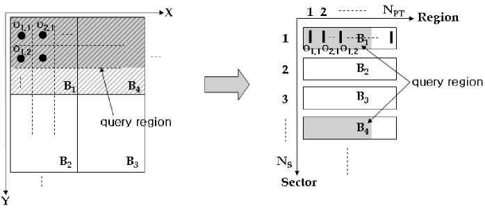
(a) A two-dimensional space.                        (b) The RS model.

Figure 15: The query region to be retrieved in Spatial-Parallel.

Here, we use two physical database design techniques to reduce the number of seek operations during query processing. First, in the partitioning step, we set the aspect ratio of a block ($BlockAspectRatio$) to be the weighted average aspect ratio of a query region defined as $QueryAspectRatio=\frac{\sum_{i}\,(f_{i}\times QueryResionSize_{i_{x}})}{\sum_{i}\,(f_{i}\times QueryResionSize_{i_{y}})}$, where $f_{i}$ is the query frequency. It has been proven by Lee et al. [11] that the number of blocks in $QueryBlockSet$ is minimized when this condition is met. Second, in the ordering step, we use the Hilbert order as the space filling curve. The more contiguously the simultaneous-access sector groups corresponding to $QueryBlockSet$ are placed, the fewer seek operations occur during query processing. Here, the degree of clustering of the blocks in $QueryBlockSet$ is dependent on the space filling curve to be used. It is known that the Hilbert order achieves the best clustering [13].

Spatial-Parallel is a new data placement technique that focuses on parallelism, while Spatial-Sequential-Yu focuses on reducing the number of seek operations as in the traditional disk-based approach.

6.2.3 Comparison between Spatial-Sequential-Yu and Spatial-Parallel

The parameters affecting the retrieval time in data placements for two-dimensional spatial data are the size and the aspect ratio of the query region. In this section, we compare the retrieval time of Spatial-Sequential-Yu and Spatial-Parallel by using Equation (32). Table 6 summarizes the notation to be used for analyzing the retrieval time.

Table 6: The notation for analyzing the retrieval time.

Symbols	Definitions
$QueryRegionSize_{x}$	the width of a query region
$QueryRegionSize_{y}$	the height of a query region
$QueryRegionSize$	the size of a query region (= $QueryRegionSize_{x}\times QueryRegionSize_{y}$)
$QueryAspectRatio$	the ratio of width to height of a query region (= $\frac{QueryRegionSize_{x}}{QueryRegionSize_{y}}$)
$\#QueryBlocks$	the number of blocks in $QueryBlockSet$

For $TotalSeekTime$, Spatial-Sequential-Yu is better than Spatial-Parallel. For Spatial-Sequential-Yu, $K_{random}=1$ because a query region is retrieved without seek operations. For Spatial-Parallel, $K_{random}\leq\#QueryBlocks$. Thus, from Equation (32), Spatial-Parallel has additional seek time of at most $\#QueryBlocks\times SeekTime_{rs}$ compared with Spatial-Sequential-Yu.

For $TotalTransferTime$, either Spatial-Sequential-Yu or Spatial-Parallel is better than the other depending on the size and aspect ratio of the query region. In Spatial-Sequential-Yu, $K_{parallel}$ decreases as $QueryRegionSize$ or $QueryAspectRatio$ gets smaller because less probe tips can be used to read the tip sectors in the query region. On the other hand, in Spatial-Parallel, $K_{parallel}$ is less affected by $QueryAspectRatio$ than in Spatial-Sequential-Yu because a query region is represented as a set of simultaneous-access sector groups rather than as a rectangular region. For example, when $QueryAspectRatio$ is very small (e.g., $QueryAspectRatio=\frac{1}{16}$), in Spatial-Sequential-Yu, only a few probe tips may be used; but in Spatial-Parallel, much more probe tips will be used because objects in the query region are placed widely in the direction of the Region axis. Therefore, Spatial-Parallel has more advantage over Spatial-Sequential-Yu as $QueryRegionSize$ or $QueryAspectRatio$ gets smaller.

If $QueryRegionSize$ or $QueryAspectRatio$ decreases below a certain threshold, the retrieval time of Spatial-Parallel becomes smaller than that of Spatial-Sequential-Yu because its advantage in the transfer time more than compensates for its disadvantage in seek time. Consequently, Spatial-Parallel has the following two good characteristics: (1) the data retrieval performance is superior to that of Spatial-Sequential-Yu for highly selective queries, (2) the performance is largely independent of the aspect ratio of the query region.

7 Performance Evaluation

7.1 Experimental Data and Environment

We compare the data retrieval performance of the new data placements proposed in this paper with those of existing data placements. We use retrieval time as the measure of the performance.

7.1.1 Experiments for Relational Data

We compare data retrieval performance of the following five data placements: Relational-Parallel, Relational-Sequential-Yu, Relational-LowerBound, NSM-Griffin, and DSM-Griffin. Here, Relational-LowerBound is a virtual data placement that has a lower bound of retrieval time in the RS model (i.e., $K_{parallel}=N_{APT}$ and $K_{random}=0$). We use this data placement in order to show how close the performance of each of the other data placements is to a lower bound of the RS model. NSM-Griffin and DSM-Griffin are the data placements using NSM [15] and DSM [3] in Section 6.1.4 based on the linear abstraction proposed by Griffin et al. [6], which corresponds to the disk mapping layer of Figure 6(a). In NSM-Griffin and DSM-Griffin, $N_{APT}$ probe tips are activated for accessing data.

For experimental data, we use the synthetic relational data that is used by Yu et al. [22]. Here, we set the number of attributes of the relation to be 16 and the size of each attribute to be 8 bytes as in Yu et al. [22].

We perform two experiments for the range selection query in Equation (6.1.2). In Experiment 1, we measure the retrieval time while varying data size from 5 Mbytes to 320 Mbytes. Here, we set $N_{projection}=8$ and selectivity = 0.1. In Experiment 2, we measure the retrieval time while varying $N_{projection}$ from $1$ to $16$. Table 7 summarizes these experiments and the parameters.

Table 7: Experiments and parameters for relational data.

Experiments		Parameters
Experiment 1	comparison of data retrieval performance	data size	5 $\sim$ 320 Mbytes
	as the size of data is varied	$N_{projection}$	8
Experiment 2	comparison of data retrieval performance	data size	320 Mbytes
	as $N_{projection}$ is varied	$N_{projection}$	1 $\sim$ 16

7.1.2 Experiments for Two-Dimensional Spatial Data

Here, we compare data retrieval performance of three data placements: Spatial-Parallel, Spatial-Sequential-Yu, and Spatial-LowerBound. As in Section 7.1.1, Spatial-LowerBound is defined to be the case where $K_{parallel}=N_{APT}$ and $K_{random}=0$.

For the experimental data, we use the synthetic spatial data that is generated by the same method used by Yu et al. [21]. Here, we set the number of spatial objects to be $40,960,000$ and the size of each object to be 8 bytes.

We perform two experiments. In Experiment 3, we measure the retrieval time while varying $QueryRegionSize$ from $0.01\%$ to $10\%$ of that of the spatial data. Here, the shape of a query is a square (i.e., $QueryAspectRatio=1$). In Experiment 4, we measure the retrieval time while varying $QueryAspectRatio$ from $16$ to $\frac{1}{16}$. Here, we fix $QueryRegionSize$ to be $1\%$ of the size of the spatial data. Table 8 summarizes the experiments and the parameters.

Table 8: Experiments and parameters for two-dimensional spatial data.

Experiments		Parameters
Experiment 3	comparison of data retrieval performance	$QueryRegionSize$	$0.01\sim 10\,\%$
	as $QueryRegionSize$ is varied	$QueryAspectRatio$	1
Experiment 4	comparison of data retrieval performance	$QueryRegionSize$	1 %
	as $QueryAspectRatio$ is varied	$QueryAspectRatio$	$16\sim\frac{1}{16}$

7.1.3 An Emulator of the MEMS Storage Device

We have implemented an emulator of the MEMS storage device since a physical MEMS storage device is not available on the market yet. We have implemented an emulator of the CMU MEMS storage device using formulas and parameters proposed by Griffin et al. [6, 7]. We conduct all experiments on a Pentium 4 3.0 GHz Linux PC with 2 GBytes of main memory.

7.2 Results of the Experiments

7.2.1 Relational Data

Figure 16 shows the retrieval time of five data placements as the data size is varied . As analyzed in Section 6.1, Relational-Parallel is superior to Relational-Sequential-Yu. As the size of data is varied from 5 Mbytes to 320 Mbytes, the performance of Relational-Parallel improves from 2.6 to 4.0 times over that of Relational-Sequential-Yu. We note that the query performance of NSM-Griffin is much poorer than those of the others. This result indicates that disk mapping approaches provide relatively poor performance compared with device-specific approaches since the characteristics of the MEMS storage device are not fully utilized.

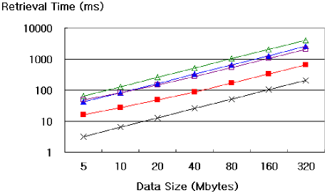
Figure 16: Retrieval time for relational data as the data size is varied ($N_{projection}=8$, selectivity = 0.1).

Figure 17 shows the retrieval time of five data placements as $N_{projection}$ is varied. As $N_{projection}$ increases, the retrieval time of Relational-Parallel increases linearly. In contrast, that of Relational-Sequential-Yu increases in a stepwise manner. The reason for this behavior is that the number of sequential scans ($\lceil\frac{m\times N_{projection}}{N_{APT}}\rceil$) in Relational-Sequential-Yu increases by an integer number. We note that Relational-Parallel is closer to Relational-LowerBound than Relational-Sequential-Yu. The retrieval time of NSM-Griffin is constant over all $N_{projection}$ because it always reads all the attribute values of the relation regardless of $N_{projection}$.

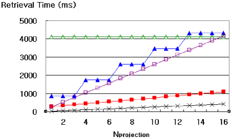
Figure 17: Retrieval time for relational data as $N_{projection}$ is varied (selectivity = 0.1).

In Figure 17, we note that the retrieval time of Relational-Sequential-Yu is slightly larger than those of NSM-Griffin and DSM-Griffin when accessing the entire relation (i.e., $N_{projection}=16$). It is because the linear abstraction proposed by Griffin et al. [6] is optimized for sequential access. The linear abstraction arranges tip sectors so as to fast access all the tip sectors in the MEMS storage device. It first accesses all the tip sectors of the first column of every region by activating another set of $N_{APT}$ probe tips, and then, accesses all the tip sectors of the second column, and so on. Thus, when accessing the entire tip sectors in the MEMS storage device, the RS model is worse than the linear abstraction in seek time. The number of seek operations of the RS model ($S_{x}\times\lceil\frac{N_{PT}}{N_{APT}}\rceil$) is larger than that of the linear abstraction ($S_{x}$).

7.2.2 Two-Dimensional Spatial Data

Figure 18 shows the retrieval time of three data placements as $QueryRegionSize$ is varied. As we argued in Section 6.2, we observe that Spatial-Parallel becomes superior to Spatial-Sequential-Yu as $QueryRegionSize$ gets smaller, that is, as the selectivity of the query gets lower. In Figure 18, as $QueryRegionSize$ is varied from $10\,\%$ to $0.01\,\%$, the performance of Spatial-Parallel improves from $1.1$ to $4.8$ times over that of Spatial-Sequential-Yu.

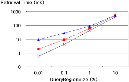
Figure 18: Retrieval time of spatial data as $QueryRegionSize$ is varied ($QueryAspectRatio=1$).

Figure 19 shows the retrieval time as $queryAspectRatio$ is varied. As we argued in Section 6.2, we observe that Spatial-Sequential-Yu degrades as $QueryAspectRatio$ decreases (i.e., $QueryRegionSize_{x}$ decreases). This is because $K_{parallel}$ in Spatial-Sequential-Yu decreases. The performance of Spatial-Parallel, however, stays largely flat regardless of $QueryAspectRatio$. Figure 19 also shows that Spatial-Parallel is close to Spatial-LowerBound.

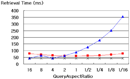
Figure 19: Retrieval time of spatial data as $QueryAspectRatio$ is varied ($QueryRegionSize=1\%$).

In Figure 19, we note that the retrieval time of Spatial-Sequential-Yu when $QueryAspectRatio=8$ is slightly larger than the time when $QueryAspectRatio=4$. It is because the case of $QueryAspectRatio=8$ requires more scan operations for accessing the query region than that of $QueryAspectRatio=4$. The case of $QueryAspectRatio=8$ requires two scans ($\lceil\frac{1820}{1280}\rceil=2$) as mentioned in Section 6.2 while the case of $QueryAspectRatio=4$ only one scan ($\lceil\frac{1280}{1280}\rceil=1$). Although the case of $QueryAspectRatio=16$ also requires two scans ($\lceil\frac{2560}{1280}\rceil=2$), it takes less retrieval time than the case of $QueryAspectRatio=8$ because the height of the query region (i.e., $QueryRegionSize_{y}$) is shorter than the case of $QueryAspect\-Ratio=8$.

8 Conclusions

In this paper, we have proposed a logical model called the RS model that abstracts the physical MEMS storage model. The RS model simplifies the structure of the MEMS storage device by rearranging its tip sectors into a virtual two-dimensional plane. As a result, the RS model represents the position of a tip sector with only two parameters while the physical MEMS storage model requires four parameters. Despite this simplification, the RS model provides characteristics for random access and sequential access (i.e., seek time and transfer rate) almost identical to those of the physical MEMS storage model.

We have presented an analytic formula for retrieval performance of the RS model in Equation (32), and then, proposed heuristic data placement strategies – Strategy_Sequential and Strategy_Parallel – based on that formula. Strategy_Parallel intends to maximize the number of probe tips to be used while Strategy_Sequential intends to minimize the number of seek operations.

By using those strategies, we have derived data placements for relational data and two-dimensional spatial data. We have identified that data placements derived by Strategy_Sequential are in effect identical to those in Yu et al. [21, 22] and that those derived by Strategy_Parallel are new ones discovered. Further, through extensive analysis and experiments, we have compared the retrieval performance of our new data placements with those of existing ones. Experimental results using relational data of 320 MBytes  show that Relational-Parallel improves the performance by up to 4.0 times (where $N_{projection}=8$ and the query selectivity = 0.1) compared with Yu et al. [22] (Relational-Sequential-Yu). This performance gain would be even higher for smaller query selectivities. Experimental results using two-dimensional spatial data of 328 MBytes  also show that Spatial-Parallel improves data retrieval performance by up to 4.8 times (where $QueryRegionSize=0.01\,\%$ and $QueryAspectRatio=1$) compared with Yu et al. [21] (Spatial-Sequential-Yu). Furthermore, these improvements are expected to become more marked as the size of the data grows, reflecting the strength of our model.

Overall, these results indicate that the RS model is a new logical model for the MEMS storage device that allows users to easily understand and effectively use this rather complex device.

9 Acknowledgement

We would like to thank Dr. Young-Koo Lee of Kyung Hee University in Korea for his helpful advice and discussions. This work was supported by the Korea Science and Engineering Foundation (KOSEF) grant funded by the Korea government(MEST) (No. R0A-2007-000-20101-0).

References

- [1] Ban, A., Flash File System, US patent 5404485, 1995.
- [2] Carley, L. R., Ganger, G. R., and Nagle, D. F., “MEMS-Based Integrated-Circuit Mass-Storage Systems,” Communications of the ACM (CACM), Vol. 43, No. 11, pp. 73–80, Nov. 2000.
- [3] Copeland, G. P. and Khoshafian, S. F, “A Decomposition Storage Model,” In Proc. Int’l Conf. on Management of Data, ACM SIGMOD, pp. 268–279, Austin, Texas, May 1985.
- [4] Dramaliev, I. and Madhyastha, T., “Optimizing Probe-Based Storage,” In Proc. 2nd USENIX Conf. on File and Storage Technologies (FAST), San Francisco, California, Mar. 2003.
- [5] Gal, E. and Toledo, S., “Algorithms and Data Structures for Flash Memories,” ACM Computing Surveys, Vol. 37, No. 2, 2005.
- [6] Griffin, J. L., Schlosser, S. W., Ganger, G. R., and Nagle, D. F., “Operating Systems Management of MEMS-Based Storage Device,” In Proc. Symp. on Operating Systems Design and Implementation (OSDI), pp. 227–242, San Diego, California, Oct. 2000.
- [7] Griffin, J. L., Schlosser, S. W., Ganger, G. R., and Nagle, D. F., “Modeling and Performance of MEMS-Based Storage Device,” In Proc. ACM Int’l Conf. on Measurement and Modeling of Computer Systems (SIGMETRICS), pp. 56–65, Santa Clara, California, June 2000.
- [8] Hilbert, D., “Über die stetige Abbildung einer Linie auf Flächenstück,” Math Ann., Vol. 38, pp. 459–460, 1891.
- [9] Hong, Bo, Brandt, S. A., Long, D. D. E., Miller, E. L., Lin, Y., “Using MEMS-Based Storage in Computer Systems-Device Modeling and Management,” ACM Transactions on Storage, Vol. 2, No. 2, pp. 139–160, May 2006.
- [10] Jagadish, H. V., “Linear Clustering of Objects with Multiple Atributes,” In Proc. Int’l Conf. on Management of Data, ACM SIGMOD, pp. 332–342, Atlantic, NJ, May 1990.
- [11] Lee, J., Lee, Y., Whang, K., and Song, I., “A Region Splitting Strategy for Physical Database Design of Multidimensional File Organizations,” In Proc. 23th Int’l Conf. on Very Large Data Bases (VLDB), pp. 416–425, Athens, Greece, Aug. 1997.
- [12] Manning, C., YAFFS: Yet Another Flash File System, 2002, available at http://www.yaffs.net/.
- [13] Moon, B., Jagadish, H. V., Faloutsos, C., and Saltz, J.-H., “Analysis of the Clustering Properties of the Hilbert Space-Filling Curve,” IEEE Trans. on Knowledge and Data Engineering, Vol. 13, No. 1, pp. 124–141, 2001.
- [14] Orenstein, J., “Spatial Query Processing in an Object-Oriented Database System,” In Proc. Int’l Conf. on Management of Data, ACM SIGMOD, pp. 326–336, Washington, D.C., May 1986.
- [15] Ramakrishnan, R. and Gehrke, J., Database Management Systems, WCB/McGraw-Hill, 2nd ed., 2000.
- [16] Rangaswami, R., Dimitrijevic, Z., and Chang, E., “MEMS-Based Disk Buffer for Streaming Media Servers,” In Proc. Int’l Conf. on Data Engineering (ICDE), pp. 619–630, Bangalore, India, Mar. 2003.
- [17] Schlosser, S. W., Griffin, J. L., Nagle, D. F., and Ganger, G. R., “Designing Computer Systems with MEMS-Based Storage,” In Proc. 9th Int’l Conf. on Architectural Support for Programming Languages and Operating Systems (ASPLOS), pp. 1–12, Cambridge, Massachusetts, Nov. 2000.
- [18] Schlosser, S. W. and Ganger, G. R., “MEMS-Based Storage Devices and Standard Disk Interfaces: A Square Peg in a Round Hole?,” In Proc. 3rd USENIX Conf. on File and Storage Technologies (FAST), pp. 87–100, San Francisco, California, Mar. 2004.
- [19] Vettiger, P., Despont, M., Drechsler, U., Durig, U., Haberle, W., Lutwyche, M. I., Rothuizen, H. E., Stutz, R., Widmer, R., and Binnig, G. K., “The Millipede – More than One Thousand Tips for Future AFM Data Storage,” IBM Journal of Research and Development, Vol. 44, No. 3, pp. 323–340, 2000.
- [20] Wise, K. D, “Special Issue on Integrated Sensors, Microactuators, and Microsystems (MEMS),” Proceedings of the IEEE, Vol. 86, No. 8, pp. 1531–1787, Aug. 1998.
- [21] Yu, H., Agrawal, D., and Abbadi, A. E., “Exploiting Sequential Access when Declustering Data over Disks and MEMS-Based Storage,” Distributed and Parallel Databases, Vol. 19, No. 2–3, pp. 147–168, 2006.
- [22] Yu, H., Agrawal, D., and Abbadi, A. E., “MEMS-Based Storage Architecture for Relational Databases,” The VLDB Journal, Vol. 16, No. 2, pp. 251–268, 2007.
- [23] Zhu, Y., “An Overview on MEMS-Based Storage, Its Research Issues and Open Problems,” In Proc. 2nd Int’l Workshop on Storage Network Architecture and Parallel I/Os, in conjunctions with 13th Int’l Conf. on Parallel Architectures and Compilation Techniques (PACT), Antibes Juan-les-pins, France, Sept. 2004.