Finite representations of continuum environments

Abstract

Understanding dissipative and decohering processes is fundamental to the study of quantum systems. An accurate and generic method for investigating these processes is to simulate both the system and environment, which, however, is computationally very demanding. We develop a novel approach to constructing finite representations of the environment based on the influence of different frequency scales on the system’s dynamics. As an illustration, we analyze a solvable model of an optical mode decaying into a reservoir. The influence of the environment modes is constant for small frequencies, but drops off rapidly for large frequencies, allowing for a very sparse representation at high frequencies that gives a significant computational speedup in simulating the environment. This approach provides a general framework for simulating open quantum systems.

How quantum systems behave when in contact with an environment has been the subject of a tremendous amount of research (Weiss, 1993; Leggett et al., 1987; Zurek, 2003). Many interesting physical scenarios can be cast in this form, such as transport through nanoscale systems (Chen and Di Ventra, 2005), interaction between local magnetic moments and conduction electrons in the Kondo problem (Kirchner and Si, 2008), charge transfer in biomolecules (Zwolak and Di Ventra, 2008), decoherence of qubits (Merkli et al., 2007), relaxation and decay (Longhi, 2006), dissipative quantum phase transitions (Meidan et al., 2007), and the quantum-to-classical transition (Zurek, 2003). Techniques to study “open” systems thus have a wide range of applicability and influence.

Analytical techniques to study these systems are generally based on integrating out the environment (Keldysh, 1965; Kadanoff and Baym, 1962; Feynman and Vernon, 1963). However, to find solutions more often than not one has to resort to a series of uncontrolled approximations. Numerical techniques, then, are the key to accurate results for many physical systems. On the one hand, Monte Carlo simulations can be used to calculate system properties directly from the path-integral representation where the environment has been integrated out (Werner and Troyer, 2005). On the other hand, the numerical renormalization group (NRG) approach is based on simulating the system and environment by choosing a finite representation of the continuum environment (Wilson, 1975; Bulla et al., 2008). This technique uses a logarithmic discretization of the environment’s spectral density (Wilson, 1975; Bulla et al., 2008; Campo and Oliveira, 2005), which enforces a flow of the low energy spectrum as one successively incorporates lower energy degrees of freedom of the environment. However, since a variational matrix-product state (MPS) approach (Verstraete et al., 2005) does not require separating energy scales, one can ask a very fundamental question: how do different fractions of the environment influence the system’s dynamics and how can this be used to construct efficient representations of the environment?

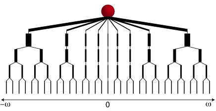
Figure 1: Schematic of a system connected to an environment. The system (top sphere) is connected to a continuum, or very finely spaced, environment, as shown on the lowest level. However, high frequency modes have less influence over the system’s dynamics, allowing for a very sparse representation by grouping modes together.

We get insight into the answer by developing a novel approach for constructing a finite representation of the environment based on the influence of environment modes (hereon just referred to as modes) at different frequency scales. We illustrate this strategy by examining a solvable model of an optical cavity mode decaying into a reservoir, where we can obtain exactly the dynamics of the system connected to a discrete environment composed of evenly spaced modes, see Fig. (1). We show that there is a frequency window centered around the system’s frequency where the mode influence is constant. However, outside this window, the mode influence drops off as $\left(\Delta/\omega^{2}\right)^{2}$, where $\Delta$ is the mode spacing and $\omega$ is the mode frequency. Thus, instead of using evenly spaced modes, we use an alternative, frequency dependent discretization $\Delta\left(\omega\right)=\Delta_{o}+d\omega^{2}$ that enforces the influence of modes at large frequencies to be constant. With this discretization, the computational cost of the simulation is significantly reduced.

We begin with a general description of the problem. A generic Hamiltonian of a system connected to an environment is

$$H=H_{S}+\sum_{k}\left(g_{k}L_{S}^{\dagger}b_{k}+g_{k}^{\star}b_{k}^{\dagger}L_{S}\right)+\sum_{k}\omega_{k}b_{k}^{\dagger}b_{k}$$ (1)

where $H_{S}$ is the system Hamiltonian and $L_{S}$ is some system operator. This represents a system connected to a non-interacting set of environment modes linearly in the environment operators. For this type of connection, the spectral function

$$J\left(\omega\right)=\sum_{k}\left|g_{k}\right|^{2}\delta\left(\omega-\omega_{k}\right)$$ (2)

completely defines the couplings and modes of the environment. Typically the spectral function is taken as some continuous function of frequency to indicate that for all practical purposes the environment is infinite compared to the system. To make simulating the system and environment a viable technique, one needs a controlled procedure for performing the mapping $J\left(\omega\right)\to\left\{\left(\omega_{i},G_{i}\right)\right\}$, where the set of environment modes $\left\{\left(\omega_{i},G_{i}\right)\right\}$ is finite and each mode $\omega_{i}$ has the associated coupling constant $G_{i}=\sqrt{J\left(\omega_{i}\right)\Delta\left(\omega_{i}\right)}$. Our starting point to find an efficient mapping is to define a measure of error for an approximation of the environment. Quite generally one is interested in system properties only, we thus use the error measure

$$\epsilon_{N}=\int_{0}^{T}dt\>\mathrm{tr}\left[\rho_{N}\left(t\right)-\rho_{ex}\left(t\right)\right]^{2}$$ (3)

where $T$ is the simulation time, $\rho_{N}$ is the reduced density matrix of the system in the presence of the finite representation (of size $N$) of the environment, and $\rho_{ex}$ is the exact reduced density matrix of the system in the presence of the continuum environment . We also define a measure of mode influence as

$$I_{N/\omega}=\int_{0}^{T}dt\>\mathrm{tr}\left[\rho_{N/\omega}\left(t\right)-\rho_{N}\left(t\right)\right]^{2}$$ (4)

where $\rho_{N/\omega}$ is the reduced density matrix in the presence of all but one, at frequency $\omega$, of the $N$ modes. The intuition behind using Eq. (4) is that modes with a small influence should be removable in a controllable manner . Having a guide such as Eq. (4) is crucial because an efficient choice of modes is going to be dependent on many factors - whether one wants equilibrium or real-time properties, the time/temperature of the simulation, the initial conditions (such as the initial excitation of the system and temperature of the environment), the Hamiltonian under consideration, etc. As a case in point, recently we showed that environments which give polynomially decaying memory kernels naturally motivate a logarithmic discretization of the kernel in time, and a property called increasing-smoothness provides a guide for more generally determining an efficient discretization (Zwolak, 2008).

To further describe and illustrate the approach, let us analyze an example of a single optical cavity mode (Carmichael, 1993) decaying into a reservoir with the Hamiltonian

$$H=a^{\dagger}B+B^{\dagger}a+\sum_{k}\omega_{k}b_{k}^{\dagger}b_{k}$$ (5)

where $B=\sum_{k}g_{k}b_{k}$. We consider the initial state defined by the correlation functions $\left\langle a^{\dagger}a\right\rangle=1$ and $\left\langle b_{k}^{\dagger}b_{k}\right\rangle=0$, and follow the evolution of the number of particles in the system, $n\left(t\right)=\left\langle a^{\dagger}a\right\rangle_{t}$, which determines the reduced density matrix of the system by $\rho\left(t\right)=\mathrm{diag}\left[n\left(t\right),1-n\left(t\right)\right]$. We also take a constant spectral function $J\left(\omega\right)=\frac{\gamma}{2\pi}$ . The exact solution in the continuum limit is $n\left(t\right)=e^{-\gamma t}$. The nice property of this model, however, is that we can solve exactly the system dynamics in the presence of discrete, evenly spaced modes (Milonni et al., 1983). The solution for the system connected to an infinite set of modes with spacing $\Delta$ is

$$n\left(t\right)=e^{-\gamma t}+\Theta\left(t-\frac{2\pi}{\Delta}\right)F\left(t,\Delta\right)$$ (6)

where $\Theta\left(t-\frac{2\pi}{\Delta}\right)$ is the step-function and the function $F\left(t,\Delta\right)$ is a sum of correction terms of order one. That is, for an infinite set of evenly spaced modes, the dynamics of the system is exact up to time $T=2\pi/\Delta$. Based on this nice property we can now examine two approaches to constructing a finite representation of the environment.

Linear Discretization - Since the simulation is exact for evenly spaced modes with $\Delta\leq 2\pi/T$, the error incurred in constructing a finite representation is going to be due to the choice of cutoff $\omega_{c}$. In the continuum limit, imposing a cutoff gives an error, from Eq. (3),

$$\epsilon_{c}=\frac{5}{2\gamma}\left(\frac{\gamma}{\pi\omega_{c}}\right)^{2}\approx\frac{5}{2\gamma}\left(\frac{\gamma T}{\pi^{2}N}\right)^{2}$$ (7)

to highest order in $1/\omega_{c}$ and the second expression is with the largest spacing possible to get a controllable error, $\Delta=2\pi/T$. This gives a direct approach to constructing a finite representation of the environment. Given the simulation time $T$, one simply uses a mode spacing of $2\pi/T$ and uses the bandwidth $\left[-\omega_{c},\omega_{c}\right]$ as a control parameter to approach the exact dynamics within time $T$. We will see below this error behavior in comparison to an alternative, influence discretization (ID).

Influence Discretization - The previous approach treats all of the modes within the bandwidth on equal footing, i.e., they all are coupled with the same strength to the system. However, it does implicitly recognize that high-frequency modes matter less, and can be truncated with a controllable error. Thus, we want to develop a way that explicitly recognizes that some frequency scales matter less, i.e., have a smaller influence on the system dynamics. To do this, let us solve for the influence, $I_{\infty/\omega}$. In the presence of an infinite bandwidth of evenly spaced modes, the equation of motion for $a\left(t\right)$, valid up to time $T=2\pi/\Delta$, is

$$\dot{a}\left(t\right)=-\gamma a\left(t\right)/2\,.$$ (8)

If we remove a single mode at frequency $\omega$, the equation of motion becomes

$$\dot{a}\left(t\right)=-\gamma a\left(t\right)/2+\frac{\gamma\Delta}{2\pi}\int_{0}^{t}dt^{\prime}\,e^{-i\omega\left(t-t^{\prime}\right)}a\left(t^{\prime}\right)\,,$$ (9)

which is again valid up to time $T=2\pi/\Delta$ and the constant $\gamma\Delta/2\pi\equiv G_{\omega}^{2}$ is the square of the coupling constant to mode $\omega$. The solution is

$$a\left(t\right)=\frac{s_{+}+i\omega}{s_{+}-s_{-}}e^{s_{+}t}-\frac{s_{-}+i\omega}{s_{+}-s_{-}}e^{s_{-}t}\,,$$ (10)

where $s_{\pm}=-\frac{1}{2}\left(\frac{\gamma}{2}+i\omega\right)\pm\frac{1}{2}\sqrt{\sigma}$ and $\sigma=\left(\frac{\gamma}{2}\right)^{2}+4\frac{\gamma\Delta}{2\pi}-\omega^{2}-i\omega\gamma$. Since we have the time evolution of the operator $a\left(t\right)$, we can now directly calculate the influence in Eq. (4). We plot this influence as a function of frequency for several times in Figure (2).

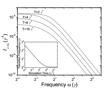
Figure 2: Single mode influence versus frequency for several simulation times. For large frequencies the influence drops off as $\left(\Delta/\omega^{2}\right)^{2}$ and for small frequencies it is constant within some frequency window. The inset shows the size of this frequency window, which drops off as $1/T$ for short times and approaches a constant for long times.

There are two crucial observations: (i) the influence is constant for small frequencies within a frequency window of width proportional to $1/T$, and (ii) for large frequencies the influence drops off as $\left(\Delta/\omega^{2}\right)^{2}$. This suggests an uneven spacing of modes that is approximately constant at small frequencies and switches over to a spacing proportional to $\omega^{2}$ for large frequencies. The simplest mode spacing that has this behavior is

$$\Delta\left(\omega\right)=\Delta_{o}+d\omega^{2}\,.$$ (11)

This spacing results in a constant influence proportional to $d^{2}$ at large frequencies . It also enables the treatment of both the truncated modes and other high frequency modes on a similar footing. That is, beyond a frequency $\omega_{c}\propto 1/d$ one can not choose any more modes and thus the parameter $d$ defines a natural cutoff, which, as we decrease $d$, we both increase the number of modes that are approximately evenly spaced at low frequency and increase the cutoff. From Eq. 7, the error due to the cutoff, which corresponds to its influence, is also proportional to $d^{2}$. Thus, the choice of mode spacing (11) enforces the high-frequency modes to be treated equally based on influence rather than based on coupling.

We can also obtain an expression for the error behavior of choosing a number of modes $N_{ID}$ based on Eq. (11). A spacing given by Eq. (11) results in $N_{ID}\approx\int_{-\omega_{c}}^{\omega_{c}}d\omega/\Delta\left(\omega\right)\propto\sqrt{N}$ modes between $-\omega_{c}$ and $\omega_{c}$ ($\propto 1/d$), compared with $N$ evenly spaced modes for the same frequency cutoff. In the process of sparsifying the high frequency modes (see Fig. (1)), $\mathcal{O}\left(\sqrt{N}\right)$ groupings of modes have to be performed, each with an error $\mathcal{O}\left(d^{2}\right)$, which are of the same order as the truncation error. Thus, the error of the ID is $\epsilon_{ID}\propto\sqrt{N}\epsilon_{c}$ . Starting from the error of the evenly spaced discretization, $\epsilon_{c}\propto 1/N^{2}$, one obtains

$$\epsilon_{ID}\propto 1/N_{ID}^{3}\,.$$ (12)

We show the results of simulations in Fig. (3) . We obtain the error scalings from Eqs. (7) and (12), and we further see that except for very short simulation times and very small number of modes, the ID needs significantly fewer modes to achieve the same accuracy. In these simulations, the computational cost to simulate an environment of $N$ modes is $N^{3}$. Thus, given a desired error, the ID reduces the computational cost from $N^{3}$ to $N_{ID}^{3}=N^{2}$.

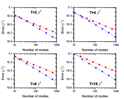
Figure 3: Simulation results for the error (Eq. (3)) versus the number of modes for several simulation times. For all the times, the evenly spaced approach (squares) gives an error that behaves as $1/N^{2}$, whereas using the ID (circles) gives $1/N_{ID}^{3}$.

Beyond solvable models - The above approach provides a general framework for simulating “open,” many-body Hamiltonians. Ultimately one wants to have an efficient, finite representation of the environment and a controllable procedure for taking the continuum limit. Therefore, we suggest taking the general Hamiltonian (1) and first examining a solvable version of it, e.g., either take the quadratic part or the part of $H_{S}$ that commutes with the system-environment interaction. With this solvable version, one can compute exactly the mode influence under similar conditions (dynamics/temperatures) to be studied with the full $H_{S}$. Then use this to construct a discretization and continuum limit procedure that will be used in the many-body case . The latter ensures that even if the discretization is not as efficient, there will still be control over the errors. Then, as with NRG, one can use the Wilson-chain construction (Wilson, 1975) directly with MPS simulations (Vidal, 2003, 2004; Zwolak and Vidal, 2004; Verstraete et al., 2004), where one can deal with both evenly or unevenly spaced modes due to the variational nature of the MPS algorithms (Verstraete et al., 2005). This will be discussed in more detail in a later publication.

Conclusions - We have developed a novel approach to constructing finite representations of continuum environments by using the single-mode influence (4) as a guide to choosing a distribution of modes. In an illustrative case, we found that the influence drops off as $\left(\Delta/\omega^{2}\right)^{2}$, which suggests a mode spacing $\Delta\left(\omega\right)=\Delta_{o}+d\omega^{2}$ . This treats the high-frequency modes, including the truncation of modes beyond the artificially imposed cutoff, on a similar footing. For this case , we showed that the computational cost to achieve a given error is reduced from $N^{3}$ to $N_{ID}^{3}=N^{2}$. It may be possible to further increase the computational efficiency by adding Markovian reservoirs to the environmental modes, where in some cases this exactly replicates the continuous environment (Garraway, 1997), or by including classical degrees of freedom in the dynamics (Sergi, 2005, 2007).