The cluster lens ACO 1703:
redshift contrast and the inner profile

Abstract

ACO 1703 is a cluster recently found to have a variety of strongly lensed objects: there is a quintuply-imaged system at $z=0.888$ and several other lensed objects from $z=2.2$ to 3.0 (the cluster itself is at $z=0.28$). It is not difficult to model the lens, as previous work has already done. However, lens models are generically non-unique. We generate ensembles of models to explore the non-uniqueness. When the full range of source redshifts is included, all models are close to $\rho\propto r^{-1}$ out to $200\;{\rm kpc}$. But if the quint is omitted, both shallower and steeper models (e.g., $\rho\propto r^{-2}$) are possible. The reason is that the redshift contrast between the quint and the other sources gives a good measurement of the enclosed mass at two different radii, thus providing a good estimate of the mass profile in between. This result supports universal profiles and explains why single-model approaches can give conflicting results. The mass map itself is elongated in the NW-SE direction, like the galaxy distribution. An overdensity in both mass and light is also apparent to the SE, which suggests meso-structure.

1 Introduction

An important prediction of hierarchical clustering of cold dark matter is a universal profile for halos. Universal profiles were originally indicated by cosmological simulations (Navarro et al., 1997; Moore et al., 1998) but more recently phenomenological models have also produced them (e.g., Austin et al., 2005; Lu et al., 2006), as have more specialized simulations (MacMillan et al., 2006). The precise form of a universal profile and the expected variation from halo to halo are still being debated; Merritt et al. (2006) discuss some competing parametrizations. A further complication arises in that infalling baryons would steepen the dark-matter profile somewhat (adiabatic contraction), but in large clusters this effect is expected to be small exterior to $\sim 20\;{\rm kpc}$ (Gnedin et al., 2004). There is general agreement that in the inner regions of clusters the dark matter profile would have $\rho\sim r^{\rm-1\ to\ -1.4}$ (Diemand et al., 2004).

Lensing is an obvious way to measure the profiles of clusters, and in this paper we will address specifically multiple-image (i.e., “strong”) lensing. Weak lensing by outer regions of clusters is also of interest (for a recent example, see Heymans et al., 2008). Other possibilities are to use generalized virial theorems and the kinematics of cluster galaxies (Łokas et al., 2006), or hydrostatic equilibrium of x-ray gas (Lemze et al., 2008). Combinations of these approaches are also possible.

Extracting a mass profile from lensing is not trivial, however. The reason is that lensing depends on integrated mass. For example, the light deflection near the Sun $4GM_{\odot}/(c^{2}R_{\odot})=1.75^{\prime\prime}$ says nothing about the mass profile of the Sun. Similarly, a single Einstein ring measures only the mass enclosed within a cylinder. Having two or more images at different radii provides some more information, but is still not sufficient to specify the mass profile, because it is possible to redistribute the mass in a way that leaves the image configuration invariant (steepness degeneracy). Much more information becomes available if the background sources are at different distances behind the lens. Light from further sources experiences a larger effective lensing deflection and hence a larger Einstein radius. Multiple Einstein radii, resulting from multiple source redshifts or “redshift contrast”, measure the mass within multiple cylinders, thus providing a robust constraint on the mass profile. ACO 1703 turns out to be a striking example of this type of constraint.

The non-uniqueness of mass models that fit a given set of observables has been much studied in lensing theory. The steepness degeneracy was discovered by Falco et al. (1985), and then rediscovered multiple times; Saha (2000) gives a short history of these (re)discoveries, and a unified picture of degeneracies then known. Further degeneracies continue to be uncovered from theory (Liesenborgs et al., 2008).

But in practice, lensing degeneracies are most likely to be noticed in the modeling process, when different kinds of models are tried out. Kochanek (1991) was the first to try a range of models and distinguish robust features from model-dependent features. Subsequent work found parameter degeneracies appearing in models in many different ways (Wambsganss & Paczynski, 1994; Bernstein & Fischer, 1999; Trotter et al., 2000). Recently Sand et al. (2008) report non-uniqueness in models of clusters.

Faced with the non-uniqueness of models, three strategies are possible.

1. One could justify the model-type being fit from astrophysical arguments, and then assume it is correct. This approach goes back to the first models of the first two known lenses (Young et al., 1981a, b). With the benefit of hindsight, we find that these pioneering models inferred correctly that the “triple-quasar” was really a quad, but predicted time delays for the double quasar several times too long.

2. One could try and introduce new information such as stellar kinematics or x-rays, as indeed Young et al. (1981b) advocated, to reduce model-dependence in the results. Czoske et al. (2008) is a recent example.

3. One can explore model degeneracies and quantify uncertainties by generating large ensembles of models, thereby also identifying the best-constrained systems.

With this background in mind, the recent discovery by Limousin et al. (2008) of 13 different multiple-image systems in ACO 1703 is very exciting. Though not a well-known cluster, ACO 1703 is a strong x-ray source (Allen et al., 1992) and hence a natural place to search for lensing. For modeling, the authors adopted strategy 1 above, and their model is a generalized NFW profile, having

$$\rho=\frac{\rho_{0}}{{\left(\frac{r}{r_{s}}\right)^{\alpha}}\left(1+\frac{r}{r_{s}}\right)^{3-\alpha}}$$ (1)

where $r$ is an elliptical radius. The normalization $\rho_{0}$ is defined indirectly in terms of the concentration $c$, such that the average density within $r=cr_{s}$ is 200 times the critical cosmological density. The models give $\alpha\simeq 1.1$, $r_{s}\simeq 170^{\prime\prime}$ or $\simeq 700\;{\rm kpc}$, and $c\simeq 3$. These results appear to verify the prediction of a universal profile, but they also raise some questions: (i) Is the model an acceptable fit to the data, according to a $\chi^{2}$ or other goodness-of-fit test? (ii) Can other, very different, models provide equally good fits? (iii) What do the fitted values of $r_{s}$ and $c$ really mean, when the data go out to only $\sim 50^{\prime\prime}$ ($\sim 200\;{\rm kpc}$)?

In this paper we analyze the same multiple-image data following strategy 3. The technique is basically the same as in our previous work on the inner profiles of J1004+411 and ACO 1689 (Saha et al., 2006). But in this work we study more carefully just where the constraints come from.

2 Modeling the cluster

2.1 The image configurations

Of the 13 multiply-imaged background objects, making a total of 42 lensed images identified by Limousin et al. (2008), some sources are probably groups of galaxies, leading to similar image systems. Of completely independent sources, there are at least six. Their image configurations are typical of cluster lenses, and can be summarized as follows.

• The quint. A five-image system (1 in the numbering system of Limousin et al., 2008) with a spectroscopic redshift $z=0.888$. The morphology is like the well-studied galaxy lens J0911+055, except that the fifth image (which in galaxy lenses is almost never observable) is here distinctly present.

• The central quads. Two four-image systems (15, 16), resulting from a two-component source. This configuration is common in galaxy lenses.

• The incipient quint. One two-image system (2), probably two-nearly merging images of a quint. The well-known galaxy lens PG1115+080 would look like this, if we knew only the two brightest images in that lens.

• The northern lemniscates. Three three-image systems (7, 8, 9), again from a multi-component source, with a typical naked-cusp or lemniscate configuration. This type of image configuration requires a strong quadrupole in the lens potential and is not shown by galaxy lenses, but is common in cluster lenses.

• The southern lemniscates. Two three-image systems (10, 11) with morphology similar to the northern lemniscates.

• The northern long arcs. Two three-image system (4, 5) which could also be lemniscates, but where modelling suggests further incipient images.

For two systems (nos. 3 and 6) in Limousin et al. (2008), the image configurations (that is, image parities, time ordering, etc.) are less clear, though both are somewhat similar to the northern lemniscates. For this reason, we do not consider these two image systems in this paper. However, model ensembles that do include these systems, with plausible image parities and time ordering, agree with the results presented here within quoted uncertainties. Many more candidate lensed objects are evident in the cluster image, and it seems likely that several more lensed systems in this cluster will be identified in the future.

Fig. 1 conveniently summarizes the image configurations, with the help of a very simple model: a cored isothermal sphere with external shear. Such a model can roughly reproduce the image positions, except that the relative sizes of the image systems are incorrect. In particular, Fig. 1 gives roughly the same size for the quint and the quad, whereas the real quint is much smaller than the quad. The reason is that the source redshift is much smaller for the quint than the quad, and this fact becomes significant below.

2.2 The modeling method

We model the cluster using the PixeLens method. The technique is described in detail in Coles (2008), and involves two ideas. (Neither of these is unique to PixeLens, though the combination is.)

1. Instead of being cast as a parameter-fitting problem, lens reconstruction is formulated as an inversion problem. The image data are treated as constraints on the mass distribution. For example, the five images of the quint are required to map to a common source position. Astrometric errors are assumed negligible. (Hence the goodness-of-fit problem does not appear, as the mass map is required to fit the image data precisely.) In addition, a mass map is required to satisfy some prior constraints. Specifically, in this work we require that (i) the mass distribution must be non-negative everywhere, (ii) the local density gradient must point within $60^{\circ}$ of the direction to the brightest cluster galaxy, and (iii) no pixel other than the central pixel can be higher than twice the sum of its neighbors.

2. Rather than a single model or a few models, an ensemble of 100 models is generated, which automatically explores degeneracies and provides uncertainties. If a single model is desired for illustration, the ensemble-average model can be used; this model is in Bayesian terms the expectation over the posterior.

Formulation of mass reconstruction in strong lensing as an inversion problem was introduced by Saha & Williams (1997) and extended to combined strong and weak lensing (Abdelsalam et al., 1998; Saha et al., 2001). These works used a form of regularization to find a single model consistent with the data and optimal according to some criterion (for example, minimal variation of $M/L$). Varying the regularization gave some idea of the uncertainties. The basic scheme has been adapted in different ways, (e.g., Bradač et al., 2005; Deb et al., 2008; Coe et al., 2008). An interesting new idea comes from Liesenborgs et al. (2007) who incorporate a constraint that additional bright images are not produced.

The technique of generating ensembles of models to explore degeneracies and estimate uncertainties (no regularization is involved) was introduced in Williams & Saha (2000) and later packaged in PixeLens (Saha & Williams, 2004), although a theoretical justification for the precise model-sampling strategy was not available until Coles (2008). Other kinds of model ensembles, involving parametric models, have also been used (Keeton & Winn, 2003; Oguri et al., 2004).

2.3 Model ensembles for ACO 1703

We now model ACO 1703 from the lensing data, considering two cases in detail: first with all the image systems discussed above included, and then with the quint excluded. The possible models in the ‘with-quint’ case are naturally a subset of the possibilities in the ‘no-quint’ case. Figs. 2 to 4 show some results from the ensemble-average models.

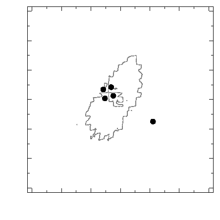
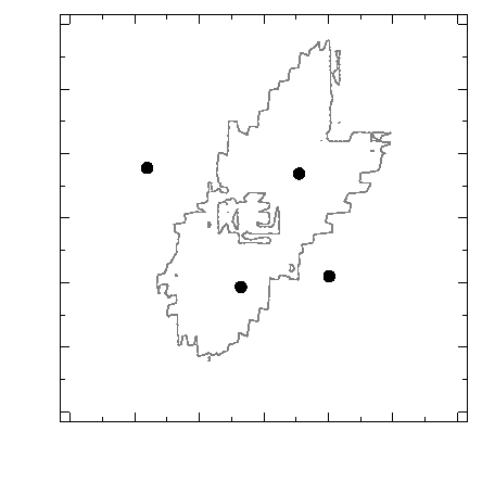
Figure 4: Critical curves of the quint and a quad, in the ensemble average model. Qualitatively, these two panels resemble the middle panels of Fig. 1. But note the size difference between the quint and the quad. Ticks are $10^{\prime\prime}$ apart.

Fig. 2 shows the ensemble-average mass maps for the two cases. Fig. 3 shows the morphologies in the PixeLens models; the with-quint case is shown, but the no-quint case is similar (apart from the quint itself). Then Fig. 4 compares the critical curves for the quint and one of the quads—these are the first and second objects shown in Fig. 3.

Qualitatively, we see that the cluster is similar to the simple model illustrated in Fig. 1, provided we take 11 o’clock in Fig. 1 as ‘north’. The arrival-time contours for the PixeLens models are like those of the simple model, as are the image configurations. The long axis of the lens is oriented perpendicular to the long direction of the quint in both cases. The critical curves are also similar, although the PixeLens curves are jagged because of pixelation. (The arrival-time contours are not jagged because they depend on integrals over the mass distribution and hence are smoother.) Clearly, these qualitative features depend only on the image identification and would appear in all models.

But of course, examining the PixeLens models in detail reveals many more features. First, we see in Fig. 2 that the with-quint and no-quint models look similar but the latter look slightly shallower. This is only true of the ensemble average; as we will see below, the no-quint ensemble contains a much larger variation of models, including steeper and shallower models than the with-quint ensemble. A second feature is that in Fig. 2 the mass contours seem to trace out the distribution of galaxies. (Recall that no information about the cluster galaxies, except the location of the brightest galaxy, was used in the modeling.) This suggests meso-structure, or extended dark-matter structure correlated with galaxies, similar to J1004+411 and ACO 1689 (Saha et al., 2007). We will not attempt to analyze this possible meso-structure in the present paper, but we will see some further indications below. A third feature is that the quint is smaller than other image systems. In Fig. 3 the quint is shown zoomed to make it comparable to the others in size, while in Fig. 4 we see that the quint has smaller critical curves. This is all simply because the quint has a smaller source redshift, and hence a smaller $D_{LS}/D_{S}$, resulting in a smaller Einstein radius. Thus, as a consequence of what we may call the redshift contrast between the quint and other sources, we have distinct Einstein radii within which the enclosed mass is well-measured. This enables a good estimate of the steepness of the mass profile, as we see below.

3 Source-redshift contrast and the inner slope

We now specialize to the radial profiles, but unlike the previous section we take the ensemble-derived uncertainties into account.

3.1 Deprojecting the mass map

From the mass map we now take the circular average to obtain $\Sigma(R)$, and then deproject to derive $\rho(r)$ by numerically solving the usual Abel integral equation. Appendix A gives details and tests of the deprojection method.

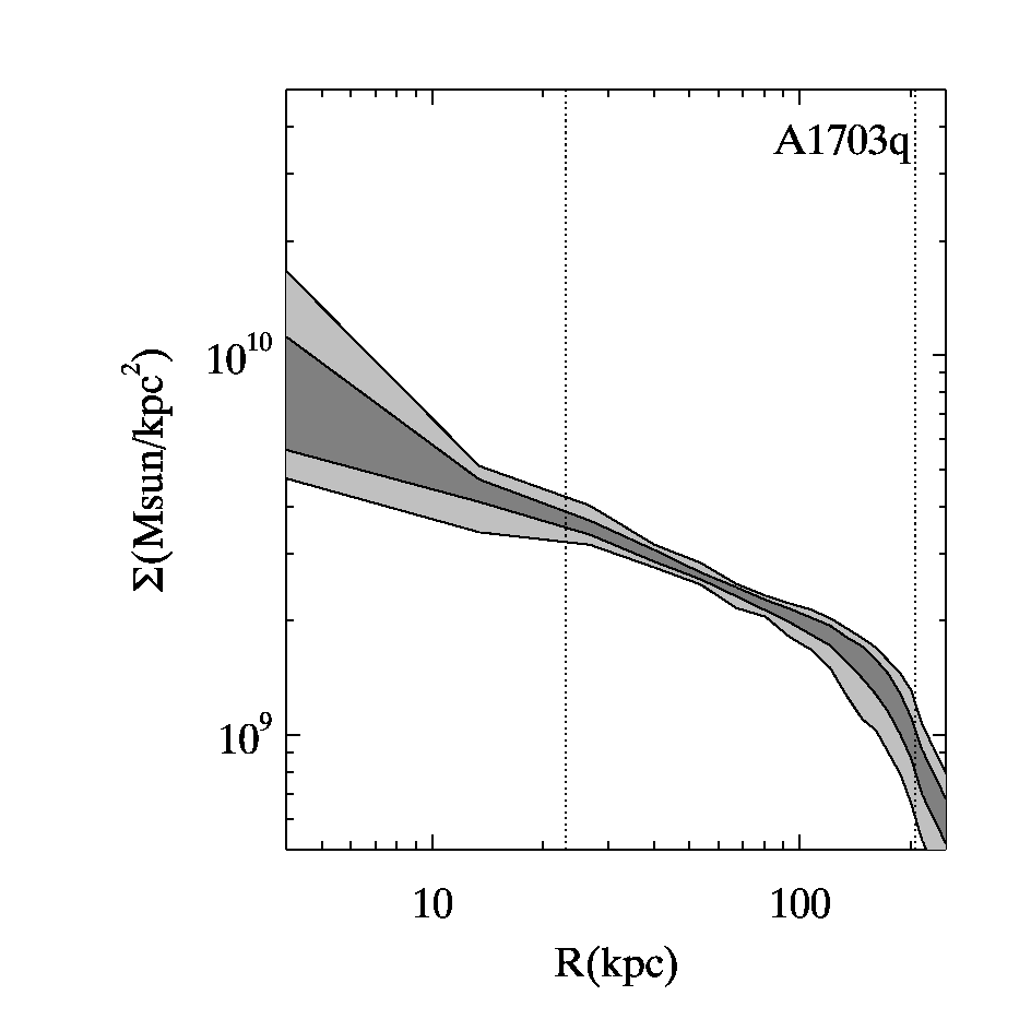
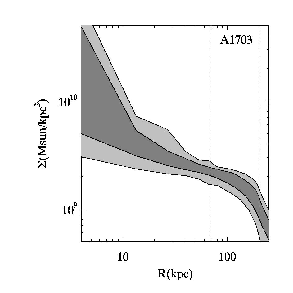
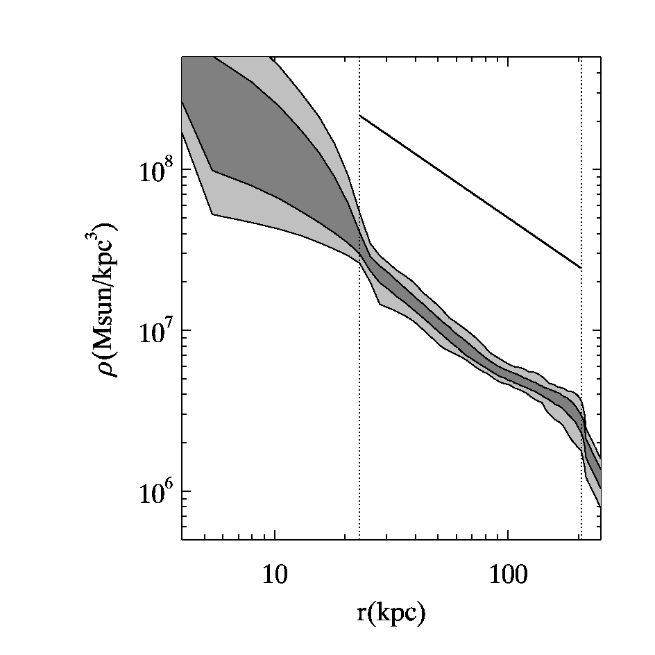
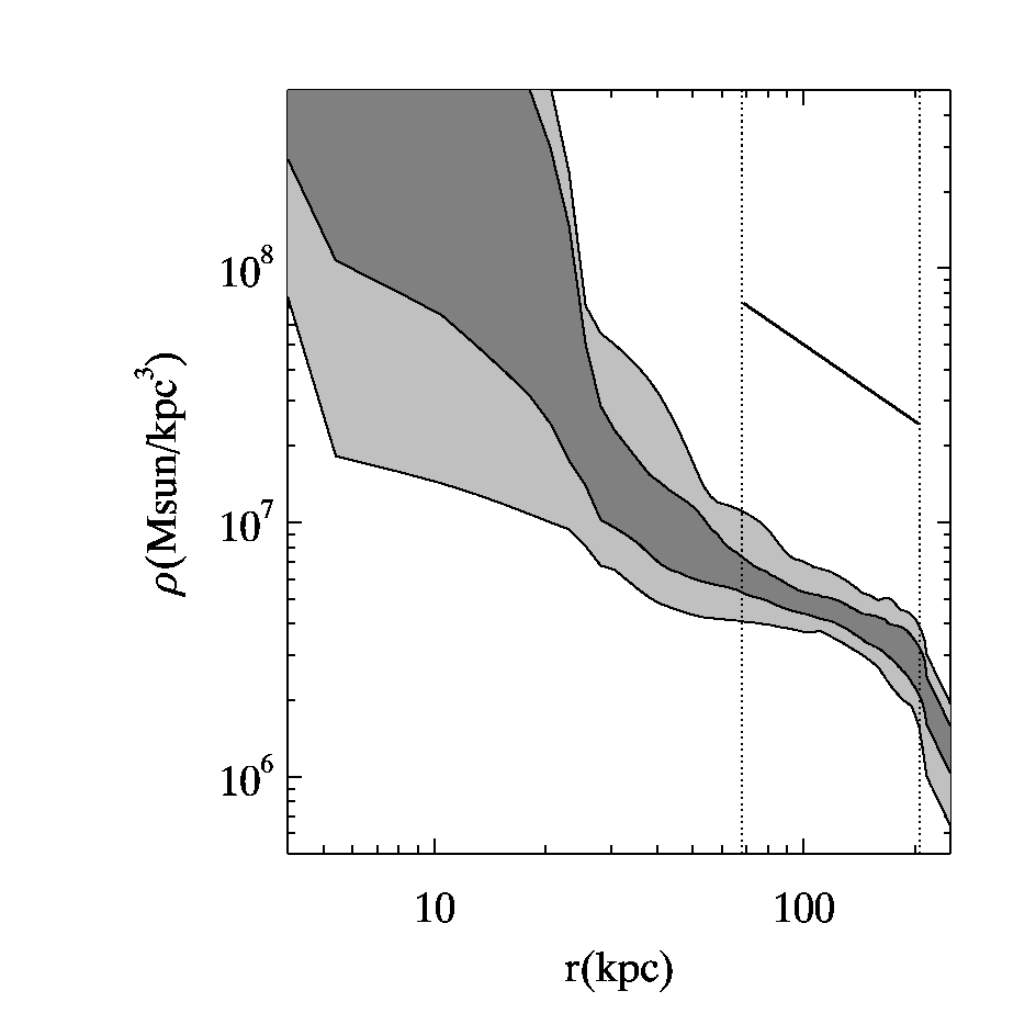
Figure 5: Surface density $\Sigma(R)$ (top panels) and deprojected density $\rho(r)$ (bottom panels) for ACO 1703. The left column is for models with the quint, the right column for models without the quint. The dark gray and light gray bands give 68% and 99% confidence intervals respectively. The vertical dotted lines are the projected radii of the inner and outermost image. The oblique line in the bottom panels shows $r^{-1}$. With the quint included, the inner profile is constrained to be quite close to $\rho\propto r^{-1}$. Without the quint, even $\rho\propto r^{-2}$ is admissible. Notice also the ‘shelf’ in $\rho(r)$ for $r\sim 100\;{\rm kpc}$, which may indicate meso-structure (see text).

Fig. 5 shows $\Sigma(R)$ and $\rho(r)$ for ACO 1703 with 68% and 99% confidence intervals, when the cluster is reconstructed with and without the quint. Notice what a difference the quint makes: without the quint, the mass profile between the innermost and outermost images could be like $r^{-1}$, but it could also be like $r^{-2}$ within the uncertainties; when the quint is included, $\rho(r)$ is inferred as close to $\propto r^{-1}$.

Note that to arrive at the conclusion that the redshift constrast reduces the available ‘model-space’, the model-ensemble strategy is essential. Within the paradigm of a single best-fit model, one cannot formulate such a conclusion. However, a single-model strategy may still provide a hint; Limousin et al. (2008) found that the slope of their best-fit model was sensitive to the redshift of the quint, and this seems to be such a hint. We emphasise that redshift contrast does not act simply by increasing the radius range. Disregarding the three innermost images of the quint gives a radius range almost identical to the no-quint case, but still adds a redshift contrast. In this case the uncertainties within the image region still shrink dramatically, as with the full quint data.

The spherically averaged density profile $\rho(r)$ in Fig. 5 also shows a ‘shelf’ (a shallowing of the log-slope) for $r\sim 100\;{\rm kpc}$. This radius corresponds to the possible meso-structure, which we have suggested above is indicated by Fig. 2. Tests (cf. Appendix A) show that deprojection of substructure will lead to a shelf or even a bump in $\rho(r)$.

It is possible to fit the spherically averaged density using the NFW-like form (1), and values like $\alpha=1$, $r_{s}=500\;{\rm kpc}$, $c=4$ (such as Limousin et al., 2008, derive) are plausible within the uncertainties. Formal least-squares parameter fits can be carried out, but are not always meaningful, because they involve the tacit assumptions that the radial bins are uncorrelated, and standard deviation over the model ensemble represent Gaussian dispersions, both of which are poor approximations. With this caveat in mind, the formal best fit to the region between the innermost and the outermost images gives $\alpha=0.95\pm 0.17$, but the scale radius $r_{s}$ and concentration $c$ are unrealistic. (The models ensemble without the quint gives $\alpha=0.5\pm 0.5$, with the formal uncertainty increasing to $\pm 1.5$ at 99% confidence.) We find systematically different parameters depending on whether the radius range with meso-structure is included in the fit: excluding the meso-structure gives $\alpha=1.22\pm 0.48$. We find smaller errors if we put priors on the scale length $r_{s}$ (as in Limousin et al., 2008), but then the best fit simply chooses the largest possible scale length.

It is easy to see why the derived $r_{s}$ is so unstable. To infer $r_{s}$ and $c$ from data interior to $r_{s}$, one would have to accurately measure the gradual steepening of $\rho(r)$. But in Fig. 5, we see that in the well-constrained region, $\rho(r)$ is probably getting shallower rather than steeper. In other words, in these data meso-structure is a stronger effect than scale radius and concentration.

It is interesting to ask whether the above meso structure can be explained simply by the dark matter associated with visible galaxies in the cluster. There are five galaxies at a projected distance of $\sim 100$ kpc that could contribute. Four lie to the south east of the cD galaxy; one to the north. We obtain a rather crude estimate of the total mass in the meso-structure by subtracting the cumulative mass of the best fit equation 1 for $r<100$ kpc from the cumulative mass of the ensemble average, and measuring the residual over the range 100 kpc$<r<$150 kpc. This gives $M_{\mathrm{meso}}=7\times 10^{12}\,M_{\odot}$, which implies an average mass per galaxy of $\sim 1.4\times 10^{12}\,M_{\odot}$. This indicates that all the mass in the meso-structure could be associated with visible galaxies (as the model of Limousin et al., 2008, assumes) but does not require it. Whether associated with the visible galaxies or not, however, the meso-structure must be a transient phenomenon. There are four cases of interest. The meso-structure could be several galaxies or one large group, or it could be viewed in projection, or really lie at $\sim 100$ kpc. If projected along the line of sight, then it is transient because it must rapidly move to larger projected radius. If it is really at $\sim 100$ kpc then, at the inferred densities of a few times $10^{6}M_{\odot}\;{\rm kpc}^{-3}$, the crossing time is $\sim 0.2$ Gyrs. If the meso structure is comprised of individual galaxies, these will rapidly phase mix; if instead the meso-structure is a large group then it will be rapidly tidally stripped, since its density is significantly lower than that of the main cluster (see e.g., Read et al., 2006). In all cases, the meso-structure will be transient.

3.2 Towards direct comparison of lenses and simulated clusters

While an inferred inner profile of $\sim r^{-1}$ provides some evidence in favor of universal profiles, it is desirable to be able to compare lens reconstructions with theory and simulations more directly. Ideally, the comparison would involve quantities clearly related to the cluster-formation process. Failing that, one would like to compare quantities that are well-constrained by the observations. Current parameterizations do not achieve either of these.

With this in mind, let us consider the lensing deflection for a source at infinity, as a function of projected radius

$$\alpha(R)=\frac{4GM(R)}{c^{2}R}.$$ (2)

Here $M(R)$ is the mass within a circle of projected radius $R$. The deflection angle can also be expressed in velocity units: if we write $\sigma^{2}(R)=c^{2}\alpha(R)/(4\pi)$ then for an isothermal sphere $\sigma$ will be the velocity dispersion.

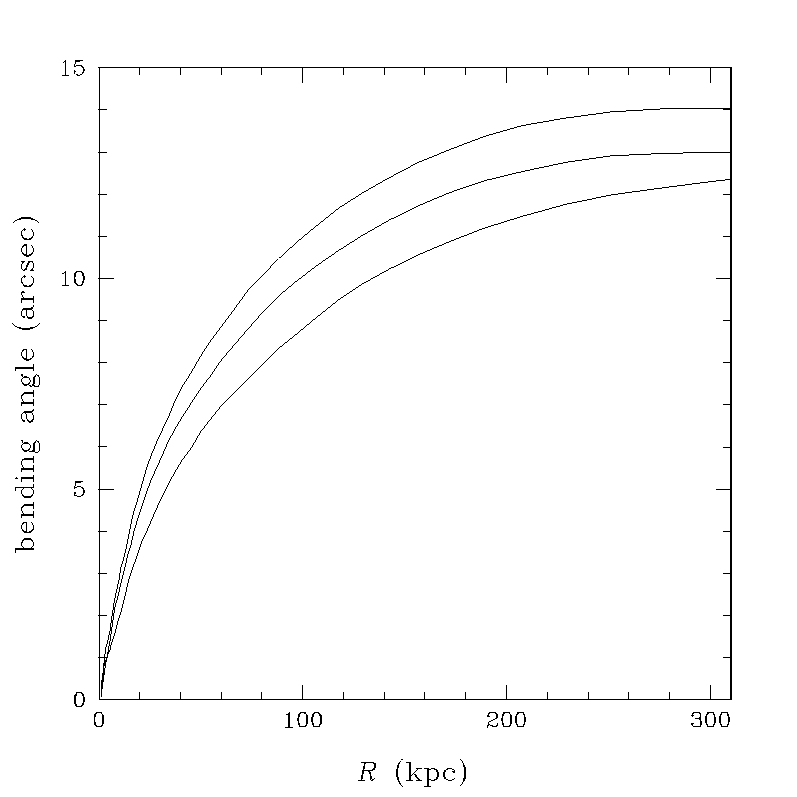
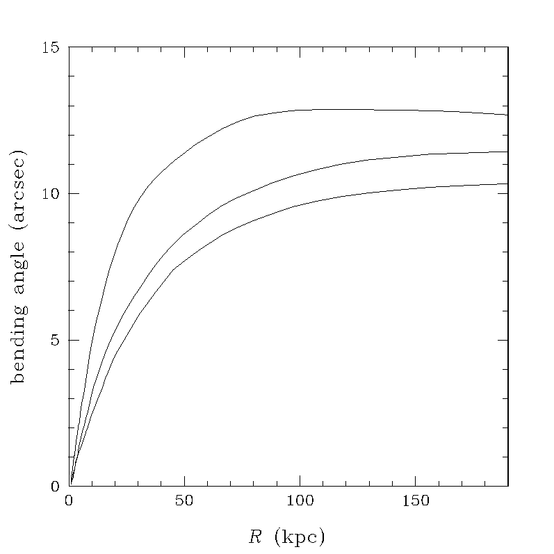
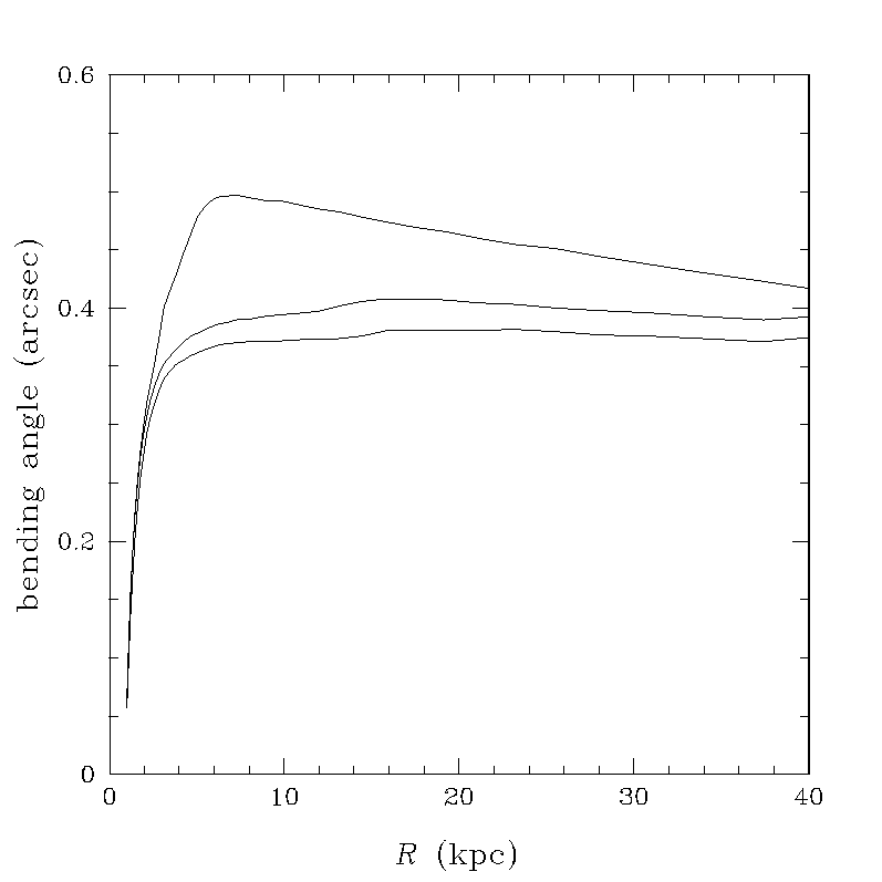
Figure 6: The bending angle $\alpha(R)$ for two simulated clusters (left and middle panels) and a galaxy (right panel), out to $\sim 25\%$ of the total mass. The three curves denote three orthogonal projections of a simulation to produce a lens.

While $\alpha(R)$ has no obvious connection to the formation process, comparing ‘bending-angle curves’ for galaxy and cluster simulations (see Fig. 6) indicates a clear qualitative difference: for a galaxy $\alpha(R)$ tends to rise steeply at first and then stay flat over an extended range, whereas for a cluster $\alpha(R)$ tends to rise and then gradually turn over. This is just another way of stating that galaxies tend to have $\sim r^{-2}$ profiles and flat rotation curves, whereas clusters tend to have shallower profiles and rising rotation curves. Put in still another way, galaxies have higher concentration than clusters.

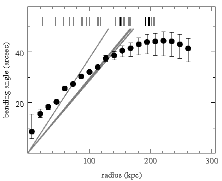
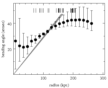
Figure 7: Deflection angle $\alpha(R)$ of the circularly averaged profile (for sources at infinity) against projected radius $R$. The upper panel come from a models with the quint included, and the lower panel from models with the quint excluded. The points show $\alpha(R)$, with 90% uncertainties derived from the ensemble, against the projected radius $R$. The barcode-like patterns show the $R$ values of individual images. The oblique lines show the critical deflection $\alpha_{\rm crit}(R)$ for each source redshift; note how the quint stands out.

In lensing, $\alpha$ is the quantity best constrained. Fig. 7 shows $\alpha(R)$ for ACO 1703, reconstructed with and without the quint. Also shown is what we may call the critical bending angle

$$\alpha_{\rm crit}(R)=\frac{D_{S}}{D_{LS}}\frac{R}{D_{L}}.$$ (3)

An intersection

$$\alpha(R_{E})=\alpha_{\rm crit}(R_{E})$$ (4)

corresponds to an Einstein ring. Strictly speaking, the Einstein radius is only defined for a perfectly circular lens, but it is useful to take (4) as a working definition of $R_{E}$.

From Fig. 7 it is clear that all the sources except the quint have a very similar $R_{E}$, whereas for the quint $R_{E}$ is significantly less. This tightly constrains $M(R)$ at two different radii, and is the reason for the constraint on the profile. Without the redshift contrast provided by the quint, the profile becomes much more uncertain, and even isothermal-type profiles are marginally permitted.

It is interesting to note that the shallower the profile, the more $R_{E}$ depends on the source redshift. This can be inferred from Fig. 7: for shallower profiles, $M(R)$ and hence $\alpha(R)$ would rise more steeply, and hence the intersections with the $\alpha_{\rm crit}$ lines would get more widely spaced.

In particular, we see $\alpha(R)$ curve and the $\alpha_{\rm crit}$ lines intersecting at $R\simeq 125\;{\rm kpc}$ for the high-redshift sources and at $R\simeq 75\;{\rm kpc}$ for the quint. Had the $\alpha(R)$ curve been constant at the $\alpha(R=125\;{\rm kpc})$ value, the $\alpha_{\rm crit}$ line for the quint would have intersected it at $R\simeq 100\;{\rm kpc}$. We may say that the characteristic size of the quint is 60% that of the other systems, whereas for an isothermal lens we would expect it to be 80% the size. Thus the simple observation that the quad is much larger than the quint is already an indicator that the profile is shallow.

More formally, let us denote the ratio $D_{LS}/D_{S}$ by $f$, and suppose that $M(R)$ mass varies in some range of $R$ as $R^{\beta}$. Substituting in Eqs. (2–4) it follows that

$$\frac{d\ln R_{E}}{d\ln f}=\frac{1}{2-\beta}.$$ (5)

The point-mass case ($\beta=0$) has the weakest dependence on the redshift contrast, while a constant-density sheet ($\beta=2$) becomes infinitely sensitive. An isothermal lens has $\beta=1$, and inner clusters are expected to locally have $\beta>1$, and hence a small change in $D_{LS}/Ds$ implies a larger change in $R_{E}$.

4 Discussion

This paper has been an analysis of the multiple-image lensing systems reported by Limousin et al. (2008) in the cluster ACO 1703, and comparison of the inner profile with what hierarchical structure formation predicts. The main conclusions are as follows.

1. It is easy to model the lens, and in simple qualitative features all models will agree. But models are highly non-unique in important details. Readers of the online version can explore models interactively: see Appendix B.

2. Robust constraints can, however, be derived from ensembles of models. We find the inner profile is well constrained and supports the prediction of universal profiles. Similar work earlier on the clusters SDSS J1004+411 and ACO 1689 led to the same conclusion (Saha et al., 2006).

3. It is possible to identify where the inner-slope constraint comes from. Behind the cluster at $z=0.28$ there is on the one hand a source at $z=0.888$ lensed into a quint, and on the other hand several sources at $z$ from 2.2 to 3.0 that are variously multiply-imaged. The redshift contrast between the quint and the other sources is responsible for the inner-slope constraint. Without the quint, any constraint on the inner slope would have been much weaker, and even an isothermal-type profile would fit.

4. The projected-density contours (see Fig. 2) correlate with the cluster galaxies. Since the mass involved is much more than the stellar mass of the galaxies, this suggests meso-structure, i.e., extended dark-matter substructure correlated with galaxies.

These results raise a further question: How can one most effectively compare a reconstructed lensing cluster with simulations and/or phenomenological models for structure? A non-parametric test would be very welcome. We suggest that the deflection angle (and specifically its redshift dependence) may form the basis for such a test. In particular, we note that the shallower the lensing profile, the more sensitive the lensed images are to source-redshift contrast.

Appendix A Deprojection of the density profile

To derive the projected density $\rho(r)$ shown in Fig. 2 we first computed the circularly-averaged $\Sigma(R)$ from the lensing mass map and then applied an Abel deprojection

$$\rho(r)=-\frac{1}{\pi}\int_{r}^{\infty}\frac{d\Sigma(R)}{dR}\frac{dR}{\sqrt{R^{2}-r^{2}}}.$$ (A1)

To evaluate the numerical derivative and then the integral, we linearly interpolate $\Sigma(R)$ up to the $R$ of the outermost image. For the contribution beyond the outermost image, we assume $\Sigma\propto R^{-2}$. This makes the total mass formally divergent, but that is harmless for the region of interest. In fact, as noted in our earlier work (Saha et al., 2006; Read et al., 2007) and also by Broadhurst & Barkana (2008), the inferred $\rho(r)$ is very insensitive to $\Sigma(R)$ for $R\gg r$, as long as $\Sigma$ is asymptotically steeper than $R^{-1}$.

Since we have an ensemble of models, we automatically derive uncertainties. Previously, we deprojected the maximum and minimum of an uncertainty band in $\Sigma(R)$ and showed the result as an uncertainty band in $\rho(r)$. This caused a problem in that the upper and lower range of $\rho(r)$ could switch, giving the illusion of zero uncertainty at certain $r$ (see the right panels of Fig. 1 in Saha et al., 2006). Here we deproject each $\Sigma(R)$ profile from the model ensemble separately, and then derive an uncertainty band in $\rho(r)$. At any $r$, the band represents the uncertainty at that $r$, marginalized over all the other radial bins.

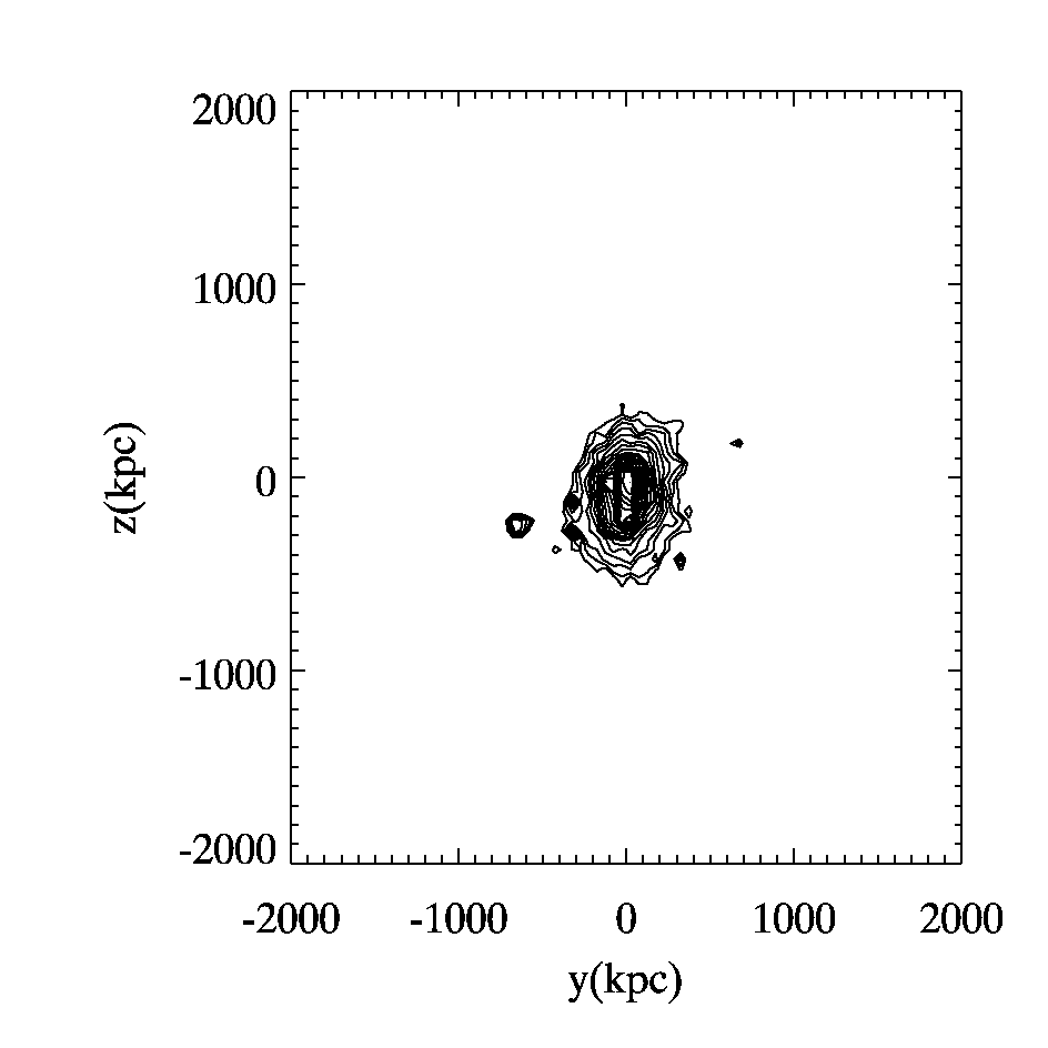
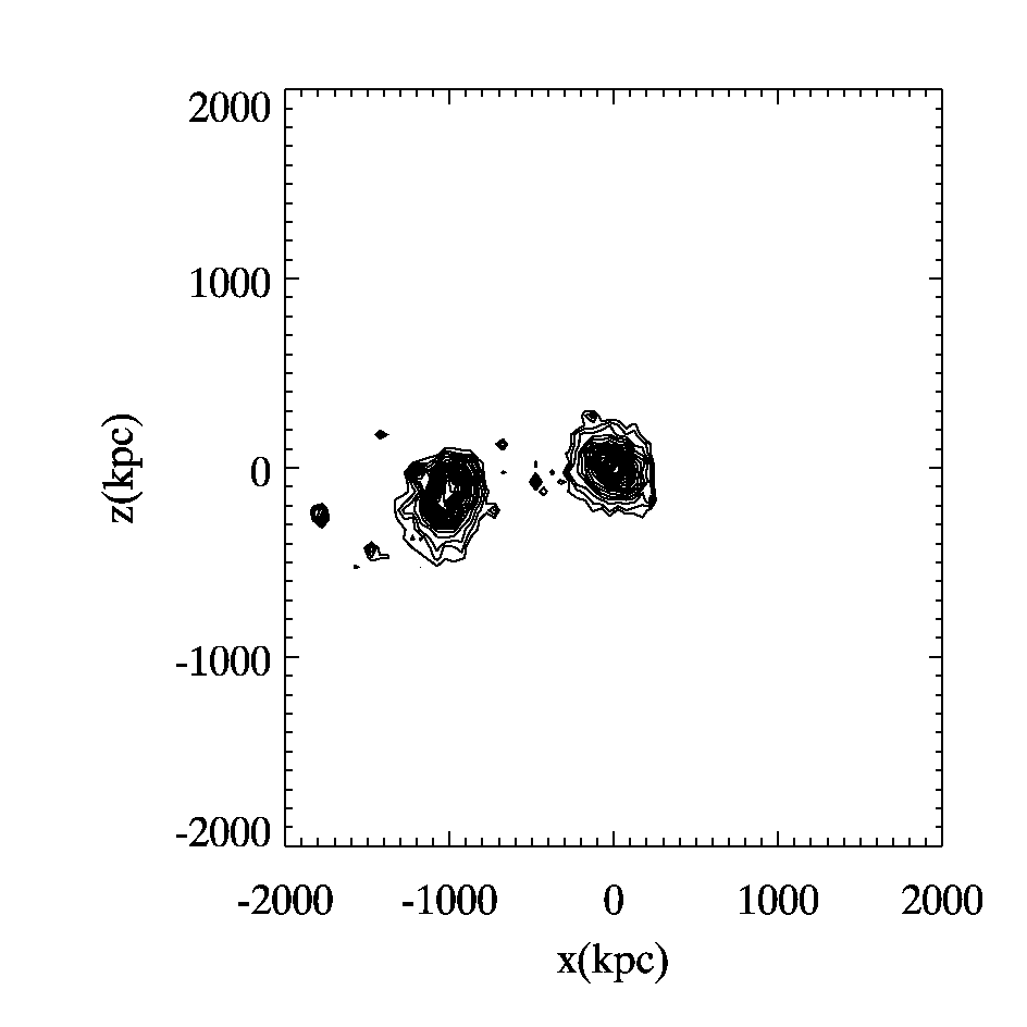
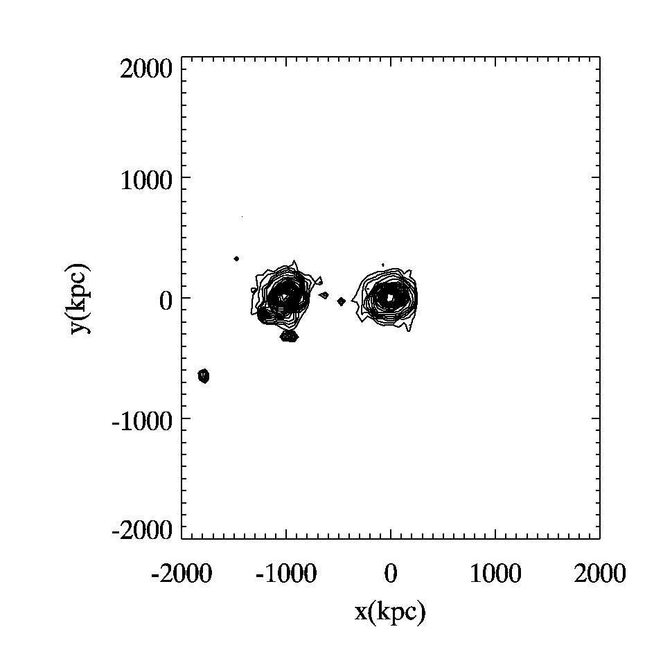
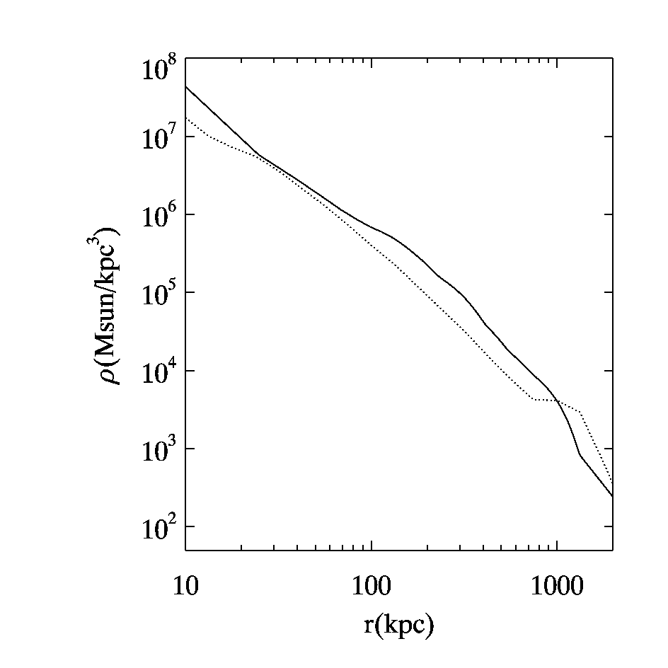
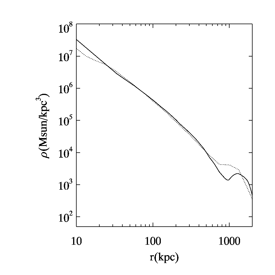
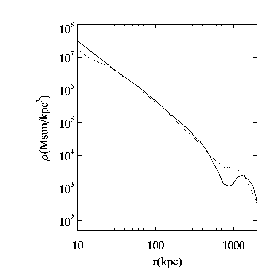
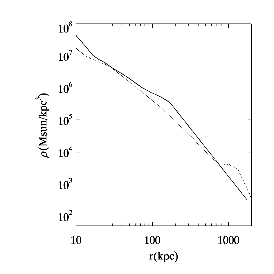
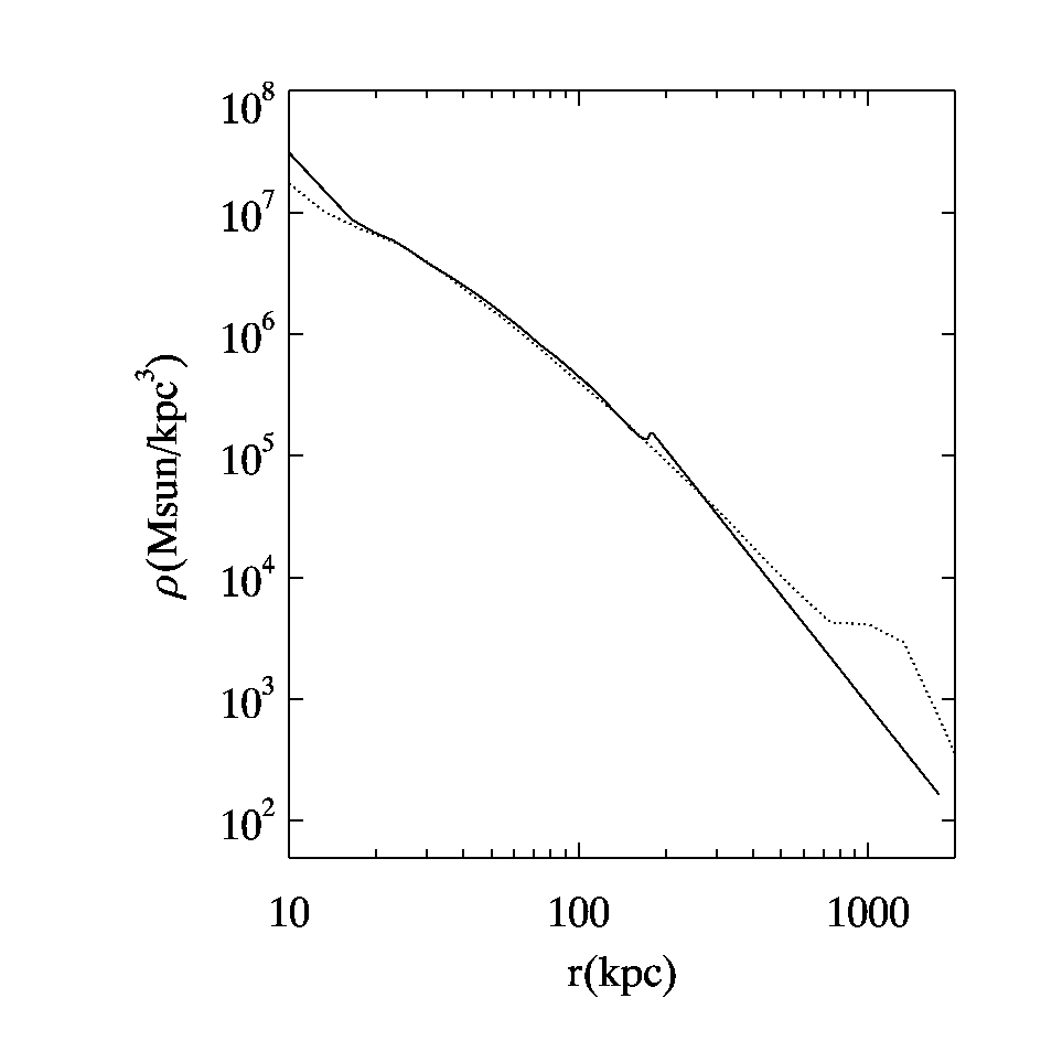
Figure 8: Test of the Abel deprojection method for an extremely non-spherical system. The upper panels show the density of an $N$-body system of two merging clusters projected along three orthogonal axes. The middle panels show the density $\rho(r)$ spherically averaged with respect to the centroid of the more massive cluster (dotted curves), and the value recovered by taking the circularly averaged projected density $\Sigma(R)$ and then deprojecting (solid curves). The lower panels are similar, except that $\Sigma(R)$ has been truncated at $200\;{\rm kpc}$ to mimic the strong lensing regime. The worst case is in the left column, when the two clusters are aligned along the line of sight.

The above procedure assumes spherical symmetry and a possible concern is that this may introduce a large systematic error if the cluster is significantly non-spherical, as ACO 1703 evidently is. To test for this, we projected and then deprojected (using the above method) 14 triaxial cluster halos taken from a cosmological $N$-body simulation. In Fig. 8 we show the worst example — where the cluster is really two merging clusters. We see that if the substructure is evident in the projection, the spherically-averaged $\rho(r)$ is mostly recovered to within the claimed uncertainties in the real cluster. The secondary cluster appears as a shelf $\rho(r)$ when it is actually a bump. The worst-case scenario is when the system is projected ‘along the barrel’ such that it appears spherical. In this case, the inferred $\rho(r)$ is overestimated by a about a factor of two.

To summarize, the errors in the deprojection are generally smaller than the uncertainty from lensing, except in the case where a major substructure is hidden along the line of sight.

Appendix B Online modeling

The online version of this paper includes the PixeLens modeling program as a Java applet. Readers can model the lens interactively within a web browser. The example input uses lower resolution than the paper, and a subset of the image systems (in fact, the six systems illustrated in Figure 3), but still enables one to verify the significance of redshift contrast. The input can be edited online, and additional data typed or pasted in.

The input syntax is as described in Saha & Williams (2004) but with one important new feature, namely multiple source redshifts. An $M$-image lens system with source redshift $z_{S}$ is input as

$$\matrix{\hbox{\tt multi}&M&z_{S}\cr x_{1}&y_{1}&p_{1}\cr&\ldots\cr x_{M}&y_{M}&p_{M}}$$

where $(x_{i},y_{i})$ are the image positions and $p_{i}$ encode the image types (1 for a mininum, 2 for a saddle point, 3 for a maximum). Coles (2008) describes recent developments of the modeling technique, including parallelism.

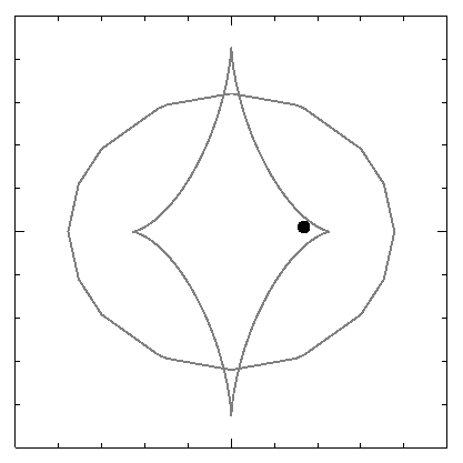
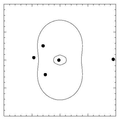
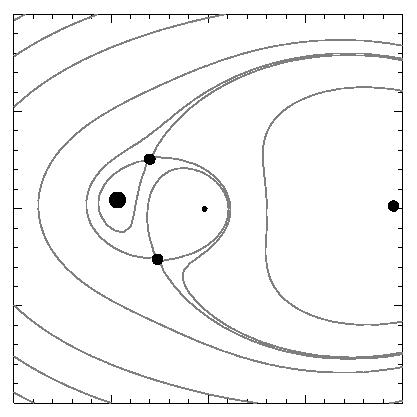
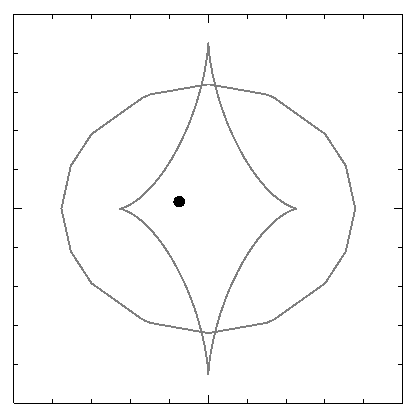
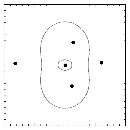
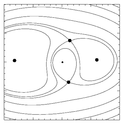
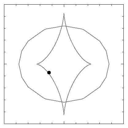
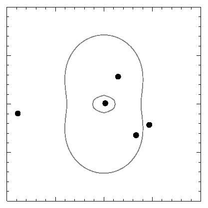
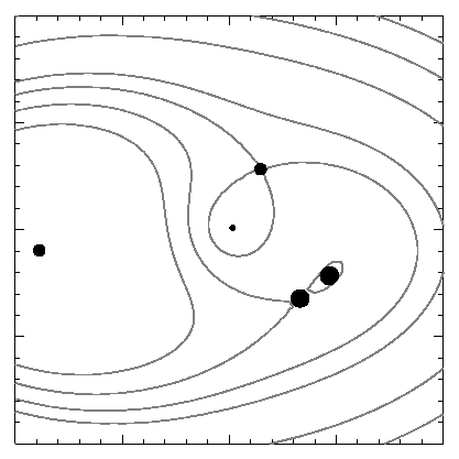
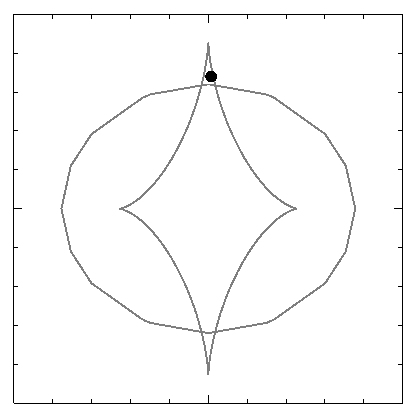
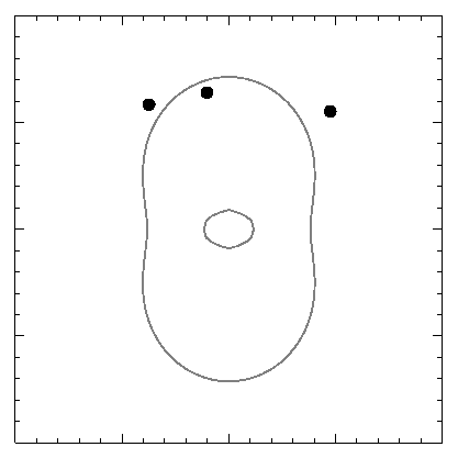
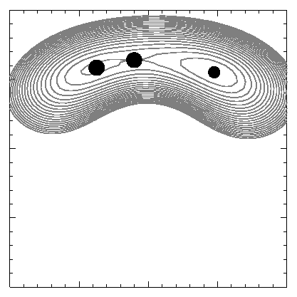
Figure 1: Qualitative summary of the image systems, using a very simple lens model. The model is a cored isothermal sphere with external shear, the lens potential being

$$\psi({\theta\kern 1.72218pt\raise 6.45831pt\hbox to0.0pt{\hss$\scriptscriptstyle\rightharpoonup$}\kern-0.04303pt})=\left(\theta_{x}^{2}+\theta_{y}^{2}+\theta_{c}^{2}\right)^{\frac{1}{2}}+{\textstyle\frac{1}{2}}\gamma(\theta_{x}^{2}-\theta_{y}^{2})$$

with $\theta_{c}=0.1$ and $\gamma=0.3$. The top row of panels corresponds to the quint, followed by the quad, the incipient quint, and the northern lemniscate. (The southern lemniscate and the northern long arc are qualitatively similar to the northern lemniscate.) In each row, the left panel shows the source position and the caustics, the middle panel shows the image positions and the critical curves, while the right panel shows the image positions and arrival-time contours. The scales are not all the same, but in all panels the distance between ticks is 0.1 in model units.

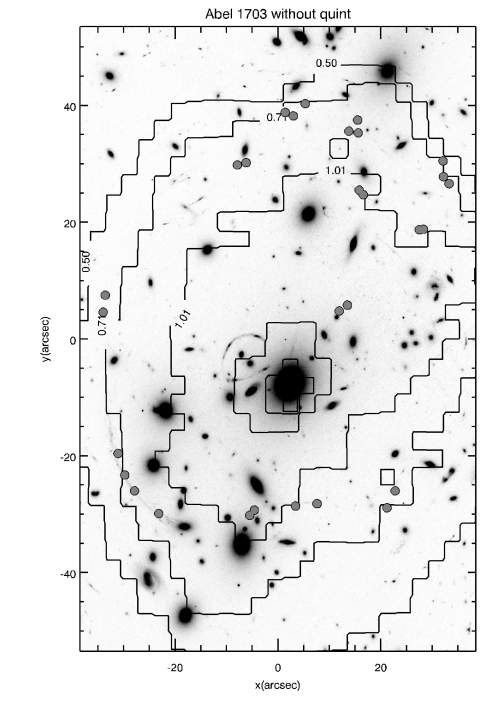
Figure 2: Mass reconstruction of ACO 1703, superimposed on an optical image of the cluster (Stott, 2007). North is up and East to the left. The two panels correspond to all image systems included (left panel) and quint excluded (right panel). Gray filled circles show image positions. Contours refer to the ensemble-average PixeLens mass model. These are labelled in units of the critical density for sources at infinity, or $3.4\times 10^{10}M_{\odot}/\rm arcsec^{2}$. The distance scale is $4.2\;{\rm kpc}/\rm arcsec$. Note the overdensities in both mass and light, especially to the SE.

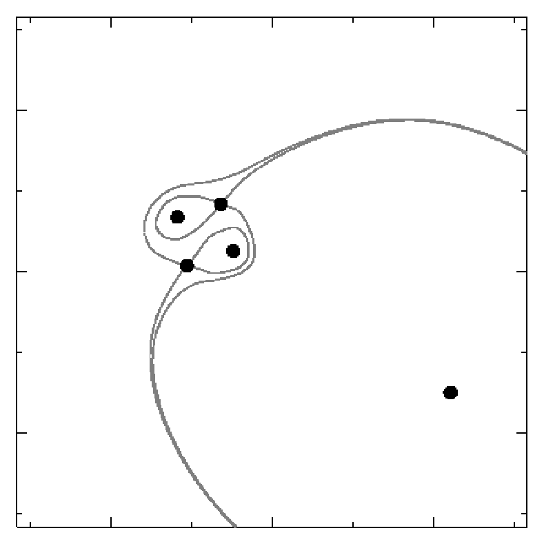
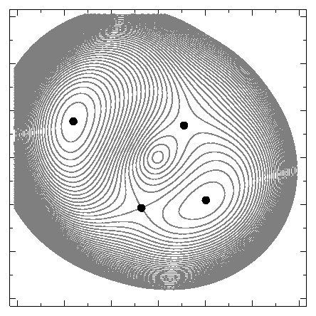
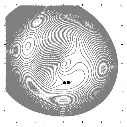
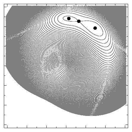
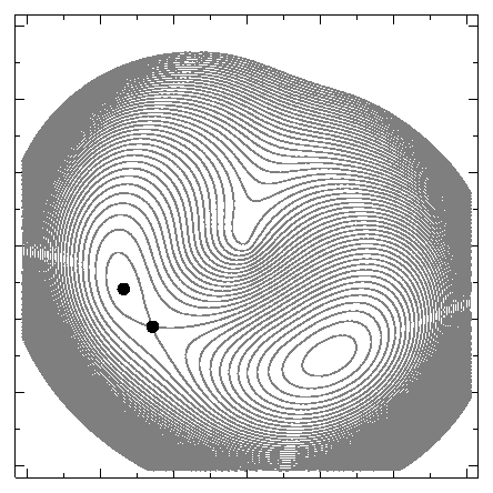
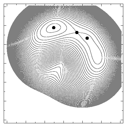
Figure 3: Arrival-time contours for six of the multiple-image systems in the ensemble-average model (left panel of Fig. 2). The panels, in reading order, refer to the quint (1 in the numbering system of Limousin et al., 2008), a quad (16), the incipient quint (2), a northern lemniscate (7), a southern lemniscate (10), and a northern long arc (4). In all panels, ticks are $10^{\prime\prime}$ apart; thus the quint is shown zoomed in. Each panel uses its own contour step, chosen to best illustrate the image configuration, but the step is always a few months of light travel time.

References

- Abdelsalam et al. (1998) Abdelsalam, H. M., Saha, P., & Williams, L. L. R. 1998, AJ, 116, 1541
- Allen et al. (1992) Allen, S. W., Edge, A. C., Fabian, A. C., Boehringer, H., Crawford, C. S., Ebeling, H., Johnstone, R. M., Naylor, T., & Schwarz, R. A. 1992, MNRAS, 259, 67
- Austin et al. (2005) Austin, C. G., Williams, L. L. R., Barnes, E. I., Babul, A., & Dalcanton, J. J. 2005, ApJ, 634, 756
- Bernstein & Fischer (1999) Bernstein, G. & Fischer, P. 1999, AJ, 118, 14
- Bradač et al. (2005) Bradač, M., Schneider, P., Lombardi, M., & Erben, T. 2005, A&A, 437, 39
- Broadhurst & Barkana (2008) Broadhurst, T. & Barkana, R. 2008, ArXiv e-prints, 0801.1875
- Coe et al. (2008) Coe, D., Fuselier, E., Benitez, N., Broadhurst, T., Frye, B., & Ford, H. 2008, ArXiv e-prints, 0803.1199
- Coles (2008) Coles, J. 2008, ApJ, 679, 17
- Czoske et al. (2008) Czoske, O., Barnabè, M., Koopmans, L. V. E., Treu, T., & Bolton, A. S. 2008, MNRAS, 384, 987
- Deb et al. (2008) Deb, S., Goldberg, D. M., & Ramdass, V. J. 2008, ArXiv e-prints, 0802.0004
- Diemand et al. (2004) Diemand, J., Moore, B., & Stadel, J. 2004, MNRAS, 353, 624
- Falco et al. (1985) Falco, E. E., Gorenstein, M. V., & Shapiro, I. I. 1985, ApJ, 289, L1
- Gnedin et al. (2004) Gnedin, O. Y., Kravtsov, A. V., Klypin, A. A., & Nagai, D. 2004, ApJ, 616, 16
- Heymans et al. (2008) Heymans, C., Gray, M. E., Peng, C. Y., van Waerbeke, L., Bell, E. F., Wolf, C., Bacon, D., Balogh, M., Barazza, F. D., Barden, M., Böhm, A., Caldwell, J. A. R., Häußler, B., Jahnke, K., Jogee, S., van Kampen, E., Lane, K., McIntosh, D. H., Meisenheimer, K., Mellier, Y., Sánchez, S. F., Taylor, A. N., Wisotzki, L., & Zheng, X. 2008, MNRAS, 385, 1431
- Keeton & Winn (2003) Keeton, C. R. & Winn, J. N. 2003, ApJ, 590, 39
- Kochanek (1991) Kochanek, C. S. 1991, ApJ, 373, 354
- Lemze et al. (2008) Lemze, D., Barkana, R., Broadhurst, T. J., & Rephaeli, Y. 2008, MNRAS, 386, 1092
- Liesenborgs et al. (2007) Liesenborgs, J., de Rijcke, S., Dejonghe, H., & Bekaert, P. 2007, MNRAS, 380, 1729
- Liesenborgs et al. (2008) —. 2008, MNRAS, 386, 307
- Limousin et al. (2008) Limousin, M., Richard, J., Kneib, J. ., Brink, H., Pello, R., Tu, H., Sommer-Larsen, J., Jullo, E., Egami, E., Michalowski, M. J., Cabanac, R., & Stark, D. P. 2008, ArXiv e-prints, 0802.4292
- Łokas et al. (2006) Łokas, E. L., Wojtak, R., Gottlöber, S., Mamon, G. A., & Prada, F. 2006, MNRAS, 367, 1463
- Lu et al. (2006) Lu, Y., Mo, H. J., Katz, N., & Weinberg, M. D. 2006, MNRAS, 368, 1931
- MacMillan et al. (2006) MacMillan, J. D., Widrow, L. M., & Henriksen, R. N. 2006, ApJ, 653, 43
- Merritt et al. (2006) Merritt, D., Graham, A. W., Moore, B., Diemand, J., & Terzić, B. 2006, AJ, 132, 2685
- Moore et al. (1998) Moore, B., Governato, F., Quinn, T., Stadel, J., & Lake, G. 1998, ApJ, 499, L5+
- Navarro et al. (1997) Navarro, J. F., Frenk, C. S., & White, S. D. M. 1997, ApJ, 490, 493
- Oguri et al. (2004) Oguri, M., Inada, N., Keeton, C. R., Pindor, B., Hennawi, J. F., Gregg, M. D., Becker, R. H., Chiu, K., Zheng, W., Ichikawa, S.-I., Suto, Y., Turner, E. L., Annis, J., Bahcall, N. A., Brinkmann, J., Castander, F. J., Eisenstein, D. J., Frieman, J. A., Goto, T., Gunn, J. E., Johnston, D. E., Kent, S. M., Nichol, R. C., Richards, G. T., Rix, H.-W., Schneider, D. P., Sheldon, E. S., & Szalay, A. S. 2004, ApJ, 605, 78
- Read et al. (2007) Read, J. I., Saha, P., & Macciò, A. V. 2007, ApJ, 667, 645
- Read et al. (2006) Read, J. I., Wilkinson, M. I., Evans, N. W., Gilmore, G., & Kleyna, J. T. 2006, MNRAS, 366, 429
- Saha (2000) Saha, P. 2000, AJ, 120, 1654
- Saha et al. (2006) Saha, P., Read, J. I., & Williams, L. L. R. 2006, ApJ, 652, L5
- Saha & Williams (1997) Saha, P. & Williams, L. L. R. 1997, MNRAS, 292, 148
- Saha & Williams (2004) —. 2004, AJ, 127, 2604
- Saha et al. (2001) Saha, P., Williams, L. L. R., & Abdelsalam, H. M. 2001, in ASP Conf. Ser. 237: Gravitational Lensing: Recent Progress and Future Go, ed. T. G. Brainerd & C. S. Kochanek, 279–+
- Saha et al. (2007) Saha, P., Williams, L. L. R., & Ferreras, I. 2007, ApJ, 663, 29
- Sand et al. (2008) Sand, D. J., Treu, T., Ellis, R. S., Smith, G. P., & Kneib, J.-P. 2008, ApJ, 674, 711
- Stott (2007) Stott, J. 2007, PhD thesis, Durham University
- Trotter et al. (2000) Trotter, C. S., Winn, J. N., & Hewitt, J. N. 2000, ApJ, 535, 671
- Wambsganss & Paczynski (1994) Wambsganss, J. & Paczynski, B. 1994, AJ, 108, 1156
- Williams & Saha (2000) Williams, L. L. R. & Saha, P. 2000, AJ, 119, 439
- Young et al. (1981a) Young, P., Deverill, R. S., Gunn, J. E., Westphal, J. A., & Kristian, J. 1981a, ApJ, 244, 723
- Young et al. (1981b) Young, P., Gunn, J. E., Oke, J. B., Westphal, J. A., & Kristian, J. 1981b, ApJ, 244, 736