Scattering and binding of different atomic species in a one-dimensional optical lattice

Abstract

The theory of scattering of atom pairs in a periodic potential is presented for the case of different atoms. When the scattering dynamics is restricted to the lowest Bloch band of the periodic potential, a separation in relative and average discrete coordinates applies and makes the problem analytically tractable. We present a number of results and features, which differ from the case of identical atoms.

The combination of external confinement and tuning of atomic levels and molecular potential curves by external fields has led to a rich variety of experiments with cold atoms, aiming at the study of formation of ultracold molecules, mean field dynamics, generation of complex many-body states, and production of quantum correlated sources of atoms. While initial studies dealt with only a single atomic species, the achievement of sympathetic cooling, mixing and observation of spatial separation of bosonic and fermionic mixtures, and formation of heteronuclear molecules with permanent dipole moments have spurred activities on mixtures of atomic species Deuretzbacher et al. (2008); Nemitz et al. (2008); Inouye et al. (2004); Stan et al. (2004); Wille et al. (2008).

In this paper, we consider the physics of a pair of atoms labeled A and B in an optical lattice consisting of three standing wave laser beams intersecting at right angles with wavelength $\lambda_{L}$. The atoms experience light induced energy shifts, which result in a cubic periodic potential $V_{\mathrm{lat},\beta}(\mathbf{x})=\sum_{i=1,2,3}V_{\beta}^{i}\sin^{2}(\pi x_{i}/a)$, where $a=\lambda_{L}/2$ is the lattice constant and $V_{\beta}^{i}$ is the lattice strength for the atomic species $\beta=A,B$ along direction $i$. The lattice strengths depend on the polarizability of the atoms as well as the amplitude and detuning of the electromagnetic field. In our numerical examples we apply the physical parameters relevant to ⁴⁰K and ⁸⁷Rb atoms, studied in Ref. Deuretzbacher et al. (2008). We take A to be ⁸⁷Rb and B to be ⁴⁰K with $V^{3}_{\mathrm{A}}=3E_{\mathrm{R,Rb}}$, $V^{1}_{\mathrm{A}}=V^{2}_{\mathrm{A}}=40E_{\mathrm{R,Rb}}$ and $V^{i}_{\mathrm{B}}=0.86V^{i}_{\mathrm{A}}$, where $E_{\rm{R},\mathrm{Rb}}={h^{2}}/{2m_{\mathrm{Rb}}\lambda_{\rm{L}}^{2}}$ is the recoil energy for rubidium.

The motion of a single atom is governed by the Hamiltonian $\mathcal{H}_{0}^{\beta}=-(\hbar^{2}/2m_{\beta})\nabla^{2}+V_{\mathrm{lat},\beta}(\mathbf{x})$, which separates into three independent one-dimensional equations, each solved by Bloch wave functions $\phi_{nq}^{\beta}(x)$, where $n$ is the band index and $q\in[-\pi/a,\pi/a]$ is the quasi-momentum. Within each band the Bloch waves can be transformed into the localized Wannier basis functions $w_{nz_{j}}^{\beta}(x)$ centered around the potential minima $z_{j}=ja$ Kohn (1959). We are interested in the quasi-one-dimensional regime, which is obtained when the lattice potential in one (longitudinal) direction is much weaker than in the two other (transverse) directions $V_{\beta}^{3}\ll V_{\beta}^{1}=V_{\beta}^{2}$. In this situation the transverse motion will be confined to the ground state of an effective harmonic oscillator with frequency $\omega_{\beta}=({\pi}/{a})\sqrt{2V_{\beta}^{1}/m_{\beta}}$ and eigenstate of motion $w^{\beta}(x)=\left({m_{\beta}\omega_{\beta}}/{\pi\hbar}\right)^{1/4}\exp(-{m_{\beta}\omega_{\beta}x^{2}}/{2\hbar})$ whenever the longitudinal motional energies are significantly below $\hbar\omega_{\beta}$. The motion is then effectively one-dimensional along the direction $x_{3}$.

The dynamics of a single atom in a one-dimensional lattice is described by the dynamical tunneling amplitudes $J_{\beta}=\langle w_{nz_{j}}^{\beta}|\mathcal{H}_{0}^{\beta}|w_{nz_{j+1}}^{\beta}\rangle$. In the following we only include nearest-neighbor tunneling, and we consider motion restricted to the lowest Bloch band ($n=1$), but our analysis and results may be generalized to higher bands and beyond nearest-neighbor tunneling Piil and Mølmer (2007).

We characterize the two-body system by a wavefunction, which is expanded on Wannier product wavefunctions $\Psi(x_{3,A},x_{3,B})=\sum_{z_{A},z_{B}}\psi(z_{A},z_{B})w_{nz_{A}}^{A}(x_{3,A})w_{nz_{B}}^{B}(x_{3,B})$ and solve for the amplitude $\psi(z_{A},z_{B})$ of finding atom A and atom B in the Wannier functions centered at the discrete sites $z_{A}$ and $z_{B}$, respectively. In this basis the two-body non-interacting Hamiltonian becomes

$${H}_{0}=-J_{A}(\Delta_{z_{A}}+2)-J_{B}(\Delta_{z_{B}}+2),$$ (1)

where $\Delta_{z}f(z)=f(z+a)+f(z-a)-2f(z)$ is the discrete Laplacian. The eigenstates of $H_{0}$ are product states

$$\psi(z_{A},z_{B})=\exp(iq_{A}z_{A})\exp(iq_{B}z_{B})$$ (2)

with energy

$$\epsilon(q_{A},q_{B})=E_{A}(q_{A})+E_{B}(q_{B}),$$ (3)

where $E_{\beta}(q_{\beta})=-2J_{\beta}\cos(q_{\beta}a)$ is the single particle energy dispersion. For convenience we put the zero of energy in the middle of the first Bloch band.

The eigenstate in Eq. (2) is a product of Bloch waves with quasi-momenta $q_{A}$ and $q_{B}$. We now change to collective $Z=(z_{A}+z_{B})/2$ and relative $z=z_{A}-z_{B}$ coordinates, and we introduce the collective $K=q_{A}+q_{B}$ and relative $q=(q_{A}-q_{B})/2$ quasi-momenta. In the special case of equal masses the collective coordinate is identical to the center-of-mass coordinate. Due to the discrete nature of the problem the Hamiltonian separates into a collective and a relative coordinate part via the Ansatz $\psi(z_{A},z_{B})=e^{iKZ}\psi_{K}(z)$. By applying ${H}_{0}$ to the product Ansatz we get $H_{0}e^{iKZ}\psi_{K}(z)=e^{iKZ}{H}^{0}_{K}\psi_{K}(z)$, where $H_{K}^{0}$ is the action of the Hamiltonian $H_{0}$ on the relative coordinate part $\psi_{K}$ given by

$$\begin{split}{H}^{0}_{K}\psi_{K}(z)=-J_{A}\left(e^{iKa/2}\psi_{K}(z+a)+e^{-iKa/2}\psi_{K}(z-a)\right)\\ -J_{B}\left(e^{-iKa/2}\psi_{K}(z+a)+e^{iKa/2}\psi_{K}(z-a)\right).\end{split}$$ (4)

Note that the relative motion Hamiltonian ${H}^{0}_{K}$ acts on components of the joint system, where $K$ has a specified value.

Unlike the case of identical atoms, where $J_{A}=J_{B}$, ${H}^{0}_{K}$ is not invariant under complex conjugation, and hence is not time-reversal invariant, for $K\neq 0$. The collective quasi-momentum is here playing a role similar to that of a classical magnetic field on the motion of electrons in an atom or a solid. As a consequence of the breaking of the time-reversal symmetry, we cannot expect the bound state wavefunctions to be real, but in further analogy with the magnetic interactions we note that time reversal of the full two-body dynamics is accompanied by a change of sign of $K$ (of the magnetic field), and hence ${H}^{0}_{K}=({H}^{0}_{-K})^{*}$. If $\psi_{-K}$ is an eigenstate of ${H}^{0}_{-K}$ then the complex conjugate, and hence time-reversed, wave function $\psi_{-K}^{*}$ is an eigenfunction of ${H}^{0}_{K}$ with the same eigenvalue.

Introducing the average and half-difference tunneling amplitudes, $J_{\Sigma,\Delta}=(J_{A}\pm J_{B})/2$, with values $J_{\Sigma}=J_{A}=J_{B}$ and $J_{\Delta}=0$ in the case of identical particles, the energies (3) can be written in the convenient form

$$\epsilon_{K}(q)=E_{K}\cos\left[(T_{K}+q)a\right],$$ (5)

which is parametrized by the collective energy

$$E_{K}=-4\sqrt{J_{\Sigma}^{2}\cos^{2}(Ka/2)+J_{\Delta}^{2}\sin^{2}(Ka/2)}$$ (6)

and by the quasi-momentum shift

$$T_{K}a=\sin^{-1}\frac{4J_{\Delta}\sin(Ka/2)}{|E_{K}|},$$ (7)

where $T_{K}a$ is taken to be in the interval $(-\pi/2,\pi/2]$ for $Ka\in(-\pi,\pi]$. The collective energy $\pm|E_{K}|$ determines the extremal values of the band of energies obtained by varying $q$, and therefore the total width of the band is $2|E_{K}|$. The continuum band is shown as a the colored region in Fig. 1(a). For the Rb-K system and our choice of optical lattice parameters the tunneling amplitudes have the values $J_{\Sigma}=0.5$kHz and $J_{\Delta}=0.5J_{\Sigma}$.

There are two significant differences from the identical particle case: (i) the width of the continuum band does not vanish for $K=\pi/a$, but maintains a finite width of $8|J_{\Delta}|$. For atom pairs with $K=0$ the width of the band is $8|J_{\Sigma}|$. (ii) The minimum and maximum of the continuum are obtained for relative quasi-momenta $q=-T_{K}$ and $q=\pm\pi/a-T_{K}$, respectively, and not, as for identical particles, at relative quasi-momenta $0$ and $\pm\pi/a$.

The finite quasi-momentum difference at the band edges, $q_{A}-q_{B}=-2T_{K}\pmod{2\pi/a}$ , appears because the energy dispersions of the atoms have different amplitudes, $2J_{\beta}$. This point is illustrated in Fig. 1(a)-(c), where the lowest energy state within the band for $Ka/\pi=0.8$ is illustrated by dots. The quasi-momenta of the individual atoms are displaced by $\pm T_{K}$ from $K/2$.

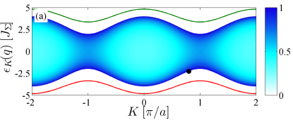
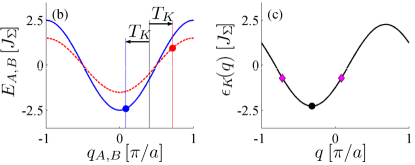
Figure 1: (a) Energy band spanned by $\epsilon_{K}(q)$ for the ratio $J_{\Delta}=0.5J_{\Sigma}$. The single atom spectra $E_{\beta}(q_{\beta})$ in (b) and the two-body spectrum $\epsilon_{K}(q)=E_{A}(K/2+q)+E_{B}(K/2-q)$ in (c) are shown for $K=0.8\pi/a$. The corresponding energy minimum $(K,q)=(0.8\pi/a,-T_{K})$ is marked by dots in all three figures and the vertical lines in (b) indicate from left to right $q_{A}$, $K/2$ and $q_{B}$. The lower and upper curve in (a) shows the bound state energy for $U=-2.7J_{\Sigma}$ and $U=2.7J_{\Sigma}$, respectively, while the shading shows the reflection coefficient for $|U|=2.7J_{\Sigma}$ [see Eq. (13)]. The significance of the diamonds in (c) is explained after Eq. (12).

The value of $T_{K}$ is depicted in Fig. 2. $T_{K}$ is an odd function of both $K$ and $J_{\Delta}$. In Fig. 2(a) the lower curve $J_{\Delta}/J_{\Sigma}=0$ corresponds to $J_{A}=J_{B}$, the identical particle case, where $T_{K}=0$ for all $K$ because both atoms have the same energy dispersion, and the upper curve $J_{\Delta}/J_{\Sigma}=1$ corresponds to $J_{B}=0$, where only atom $A$ is allowed to move, and therefore $q_{A}=K$, $q_{B}=0$ and $T_{K}=K/2$. From Fig. 2(b) we note that $T_{0}$ is always zero, and whenever $J_{A}\neq J_{B}$ we have $T_{\pi/a}=\pi/2a$ due to the symmetry of the single particle dispersions.

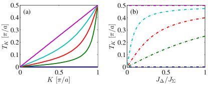
Figure 2: Shift of the relative momentum, $T_{K}$. (a) From below $J_{\Delta}/J_{\Sigma}=0,\ 0.1,\ 0.25,\ 0.5,\ 1$. (b) From below $Ka/\pi=0,\ 0.5,\ 0.8,\ 0.95,\ 1$.

So far, our analysis has only accounted for the separable state (2) of non-interacting atoms in a collective set of coordinates Note1 . In the presence of an atomic interaction depending only on the relative coordinate the separation in $z$ and $Z$ is maintained, and we now turn to the description of the dynamics and bound states of the interacting system. In the Wannier basis we assume the interaction potential, $\hat{U}$, to be on-site, i.e., of the form $U\delta_{z,0}$, where $U$ is a function of the three-dimensional background scattering length and the optical lattice parameters. The bound and scattering states are analyzed using the relative motion Green’s function for the non-interacting particles, $\hat{G}_{K}^{0}(E)=[E-\hat{H}_{0}]^{-1}$. Due to the assumption of on-site interactions, we only need to specify $G_{K}^{0}(E,z)=\langle z|\hat{G}_{K}^{0}(E)|0\rangle$ given by the Fourier transform

$$G_{K}^{0}(E,z)=\int^{\pi/a}_{-\pi/a}\frac{dq}{2\pi}\frac{ae^{iqz}}{E-E_{K}\cos((T_{K}+q)a)+i\eta}$$ (8)

of the relative quasi-momentum Green’s function, $\mathcal{G}_{K}(E;q,q^{\prime})=\delta(q-q^{\prime})/(E-\epsilon_{K}(q))$. Here $\eta$ is a positive infinitesimal added to enforce outgoing boundary conditions. By a change of coordinate $q\to q-T_{K}$ the integral is identical, except for a front factor $\exp(-iT_{K}z)$, to the one studied previously for identical particles Nygaard et al. (2008a). Hence, for energies inside the continuum band we have

$$G_{K}^{0}(E,z)=-\frac{ie^{-iT_{K}z}e^{ip|z|}}{\sqrt{E_{K}^{2}-E^{2}}},$$ (9)

where $pa=\cos^{-1}(E/E_{K})$, and outside the continuum we find

$$G_{K}^{0}(E,z)=\textrm{sgn}(E)\frac{e^{-iT_{K}z}e^{-\kappa|z|}}{\sqrt{E^{2}-E_{K}^{2}}}[-\textrm{sgn}(E)]^{z/a}$$ (10)

with $\kappa a=\cosh^{-1}|E/E_{K}|$. The Green’s function is similar to the identical particle case, except for a complex factor $e^{-iT_{K}z}$, as already mentioned, and a modified expression for $E_{K}$ (6).

We use the Dyson equation, $\hat{G}_{K}^{U}(E)=\hat{G}_{K}^{0}(E)+\hat{G}_{K}^{0}(E)\hat{U}\hat{G}_{K}^{U}(E)$, to find the interacting Green’s function

$$G^{U}_{K}(E,z)=\frac{G^{0}_{K}(E,z)}{1-UG^{0}_{K}(E,0)},$$ (11)

and the scattering wavefunction then follows from the Lippmann-Schwinger equation

$$\psi_{K}(E,z)=e^{i(p-T_{K})z}+UG_{K}^{U}(E,0)e^{-iT_{K}z}e^{ip|z|}.$$ (12)

Note that the relative quasi-momenta of the incoming $q=p-T_{K}$ and reflected $q^{\prime}=-p-T_{K}$ waves are not related in the usual way, since $q^{\prime}\neq-q$, unless $K=0$. This is explained by the degeneracy of $q$ and $q^{\prime}$ due to the symmetry of the $\epsilon_{K}(q)$ around the minimum energy state $q=-T_{K}$, as indicated by the diamonds in Fig. 1(c).

From the scattered wave in Eq. (12) we can identify the scattering amplitude $f(E,K)=UG_{K}^{U}(E,0)$ and thereby the reflection coefficient

$$R(E,K)=|f(E,K)|^{2}=\frac{U^{2}}{E_{K}^{2}-E^{2}+U^{2}},$$ (13)

which is indicated by the shading in Fig. 1(a). It reaches unity at the continuum boundaries, where the density of state diverges, and its minimum at the center of the energy band. The transmission coefficient $T(E,K)=1-R(E,K)$ might be probed in scattering experiments or measured spectroscopically by radiative coupling of a bound molecular state to the continuum Nygaard et al. (2008a). In the latter case a deep-lying, tightly confined molecular state $|i\rangle$ is coupled to the continuum by some transition operator $\hat{T}$, and the transition probability is then given by

$$|\langle\psi_{K}(E)|\hat{T}|i\rangle|^{2}\propto|\psi_{K}(E,z=0)|^{2}=T(E,K).$$ (14)

The system supports bound states of the atoms, found as the poles of the scattering amplitude, $f(E,K)$, with energy $E_{b}^{0}=\textrm{sgn}(U)\sqrt{E_{K}^{2}+U^{2}}$. As for identical particles, we find a bound state below the continuum in the case of attractive interactions and a repulsively bound state Winkler et al. (2006) above the continuum in the case of $U>0$. The corresponding bound state wavefunction of relative motion is given by $G_{K}^{0}(E_{b}^{0},z)$, Eq. (10), up to a normalization factor. This function is exponentially decaying with $|z|$.

The bound state wavefunctions are complex with a spatial phase variation of the relative motion, c.f Eq. (10). This is in agreement with our earlier discussion of the lack of time-reversal invariance of the relative motion Hamiltonian restricted to fixed values of $K$. While such a complex phase variation may give the impression that one particle is passing by the other one over and over again within the exponential envelope of their relative motional state, the two atoms are actually moving with the same group velocity. To see this, we recall that the bound states above (below) the continuum have predominantly the quasi-momentum components of the noninteracting continuum states close to the upper (lower) band edge. This implies that the quasi-momentum distribution of the attractively and repulsively bound states are peaked around $q=-T_{K}$ and $q=\pm\pi/a-T_{K}$, respectively, which can also be recognized directly from Eq. (10). For these eigenstates of $H_{0}$ a simple calculation

$$\frac{\partial\epsilon_{K}(q)}{\partial q}=\frac{\mathrm{d}E_{A}}{\mathrm{d}q_{A}}\frac{\mathrm{d}q_{A}}{\mathrm{d}q}+\frac{\mathrm{d}E_{B}}{\mathrm{d}q_{B}}\frac{\mathrm{d}q_{B}}{\mathrm{d}q}=\hbar(v_{A}-v_{B})$$ (15)

relates the group velocities $v_{\beta}$ of species $\beta$ to the derivative of the energy dispersion. At the band edges $\epsilon_{K}(q)$ reaches its extrema, i.e., ${\partial\epsilon_{K}(q)}{\partial q}=0$, exactly when $q=-T_{K}$ or $q=\pm\pi/a-T_{K}$, and the group velocities agree for these relative quasi-momentum components. Furthermore, since $\epsilon_{K}(q)$ is an even function around $q=-T_{K}$, the derivative and hence the difference in group velocity $v_{A}-v_{b}$ is odd. If we return to the scattering state in Eq. (12), we therefore observe that the difference in group velocity always changes sign when the wave is reflected.

In Fig. 3 we show the quasi-momentum distribution of the two components $A$ and $B$ for both a repulsively (a) and attractively (b) bound atom pair Note2 . We have assumed a Gaussian distribution in $K$ with center $\bar{K}=0.8\pi/a$ and standard deviation $\sigma_{K}=0.1\pi/a$. Clear peaks appear at $q_{A}+q_{B}=\bar{K}$ and $q_{A}-q_{B}=-2T_{\bar{K}}$ as marked by crosses. Here $T_{\bar{K}}=0.32\pi/a$, corresponding to $(q_{A},q_{B})=(0.08\pi/a,0.72\pi/a)$ in the attractive case (a), while $(q_{A},q_{B})=(-0.92\pi/a,-0.28\pi/a)$ in the case of repulsion (b).

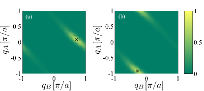
Figure 3: Quasi-momentum probability distribution in units of $(a/2\pi)^{2}$ for the species $A$ and $B$ in a bound state with (a) $U=-2.7J_{\Sigma}$ and (b) $U=+2.7J_{\Sigma}$.

We suggest measuring the wave number shift $T_{K}$ by rapidly turning off the lattice potential, because an adiabatic ramp down would alter $J_{\Delta}$ and thereby $T_{K}$. The shift of the main peak in the momentum spectrum of each individual species is then given by $K/2\to K/2\pm T_{K}$ for $U<0$ and $K/2\to K/2\pm T_{K}\pm\pi/a$ for $U>0$. The case with attractive interaction is shown in Fig. 4(a) with the same spread in $K$ as in Fig. 3. In an experiment the difference between the main momentum peaks of the two species is $2T_{K}$. The case with repulsive interaction is shown in Fig. 4(b). Alternatively, if the species are held by different lasers, the lattice may be turned off adiabatically in a controlled fashion that keeps the difference in the tunneling amplitudes $J_{\Delta}$, and hence $T_{K}$, fixed.

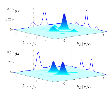
Figure 4: Momentum probability distribution in units of $(a/2\pi)^{2}$ for a pair of (a) attractively bound and (b) repulsively bound atoms with the same parameters as in Fig. 3. The solid lines show the projected probability of each species $P(k_{A,B})$ in units $a/2\pi$.

In this paper we have presented an analytical description of both the dynamics and the bound states of an atom pair of different atoms in a quasi-one-dimensional lattice. We suggest several experiments to probe our model. The transmission coefficient, Eq. (13), can be probed either by a collision experiment or by RF coupling a strongly bound state to the structured continuum, and the wave number shift $T_{K}$ of the bound states can be measured from the momentum distribution in a time of flight experiment.

We have assumed the two atoms to be in the same Bloch band, but they could just as well be in different Bloch bands, which also gives rise to different tunneling amplitudes $J_{A}\neq J_{B}$. In addition, the model can be extended to describe two-channel magnetic Feshbach resonances as outlined for identical particles in Refs. Nygaard et al. (2008b, a) by replacing $E_{K}$ and by modifying the Green’s function in those papers in accordance with our Eqs. (6), (9) and (10).

References

- Deuretzbacher et al. (2008) F. Deuretzbacher, K. Plassmeier, D. Pfannkuche, F. Werner, C. Ospelkaus, S. Ospelkaus, K. Sengstock, and K. Bongs, Phys. Rev. A 77, 032726 (2008).
- Nemitz et al. (2008) N. Nemitz, F. Baumer, F. Münchow, S. Tassy, and A. Görlitz, eprint arXiv: 0807.0852 (2008).
- Inouye et al. (2004) S. Inouye, J. Goldwin, M. L. Olsen, C. Ticknor, J. L. Bohn, and D. S. Jin, Phys. Rev. Lett. 93, 183201 (2004).
- Stan et al. (2004) C. A. Stan, M. W. Zwierlein, C. H. Schunck, S. M. F. Raupach, and W. Ketterle, Phys. Rev. Lett. 93, 143001 (2004).
- Wille et al. (2008) E. Wille, et al., Phys. Rev. Lett. 100, 053201 (2008).
- Kohn (1959) W. Kohn, Phys. Rev. 115, 809 (1959).
- Piil and Mølmer (2007) R. Piil and K. Mølmer, Phys. Rev. A 76, 023607 (2007).
- (8) An alternative collective coordinate approach to the solution of the two-particle problem is presented in J.-P. Martikainen, e-print arXiv:0808.0646.
- Nygaard et al. (2008a) N. Nygaard, R. Piil, and K. Mølmer, Phys. Rev. A 78, 023617 (2008).
- Winkler et al. (2006) K. Winkler, G. Thalhammer, F. Lang, R. Grimm, J. Hecker Denschlag, A. J. Daley, A. Kantian, H. P. Büchler, and P. Zoller, Nature 441, 853 (2006).
- (11) Care is needed when obtaining Fig. 3, because Eq. (7) is specified with the choice of Brillouin zone , which is rotated by compared to .
- Nygaard et al. (2008b) N. Nygaard, R. Piil, and K. Mølmer, Phys. Rev. A 77, 021601(R) (2008b).