A note on black hole masses estimated by the second moment in Narrow Line Seyfert 1 Galaxies

Abstract

The second moment of the H$\beta$ emission line is calculated for 329 narrow line Seyfert 1 galaxies (NLS1s) selected from the Sloan Digital Sky Survey (SDSS), which is used to calculate the central supermassive black hole (SMBHs) mass of each. We find that the second moment depends strongly on the broader component of the H$\beta$ line profile. We find that for the NLS1s requiring two Gaussians to fit the H$\beta$ line the mean value of the SMBH mass from the H$\beta$ second moment is larger by about 0.50 dex than that from the full width at half maximum (FWHM). Using the gas velocity dispersion of the core/narrow component of [O iii] $\lambda$ 5007 to estimate the stellar velocity dispersion, $\sigma_{*}$, the new mass makes NLS1s fall very close to the $M_{\rm BH}-\sigma_{*}$ relation for normal AGNs. By using $\sigma_{*}$ measured directly from SDSS spectra with a simple stellar population synthesis method, we find that for NLS1s with mass lower than $10^{7}M_{\odot}$, they fall only marginally below the $M_{\rm BH}-\sigma_{*}$ relation considering the large scatter in the mass calculation.

1 INTRODUCTION

Narrow line Seyfert 1 galaxies (NLS1s) are thought to be a special subclass of active galactic nuclei (AGNs) harboring relatively small but growing supermassive black holes ($M_{\rm BH}$ , SMBHs), compared to other broad line Seyfert 1 galaxies (BLS1s; e.g., Osterbrock & Pogge 1985; Boller et al. 1996; Mathur et al. 2000). Whether NLS1s follow the well-known $M_{\rm BH}-\sigma_{*}$ (or $M_{\rm BH}-L_{\rm bulge}$) relation defined in inactive galaxies is a question open to debate, where the stellar velocity dispersion ($\sigma_{*}$) is measured at an eighth of the effective radius of the galaxies (e.g., Tremaine et al. 2002; Mathur Kuraszkiewicz & Czerney 2001; Bian & Zhao 2004; Grupe & Mathur 2004; Botte et al. 2005; Barth et al. 2005; Watson Mathur & Grupe 2007; Ryan et al. 2007; Komossa & Xu 2007). It remains also a question for other types of AGNs (e.g., Nelson et al. 2000; Greene & Ho 2006; Shen et al. 2008; Woo et al. 2008). In investigating the $M_{\rm BH}-\sigma_{*}$ relation for NLS1s or/and other AGNs, the method of determinging $M_{\rm BH}$ and $\sigma_{*}$ is very important.

The central SMBH mass in AGNs is a key parameter to understand the nuclear energy mechanism as well as the cosmic formation and evolution of SMBHs and their host galaxies (e.g. Rees 1984; Gebhardt et al. 2000; Ferrarese & Merrit 2000; Tremaine et al. 2002). In the past two decades, there has been striking progress in finding more reliable methods to calculate SMBHs masses in AGN through the line width, $\Delta V$, of H$\beta$ (or H$\alpha$, Mg ii , C iv ) from the broad line region (BLR) and the BLR size, $R_{\rm BLR}$ (e.g., Kaspi et al. 2000; McLure & Dunlop 2004; Bian & Zhao 2004; Peterson et al. 2004; Greene & Ho 2005b).

Introducing the scaling factor, $f$, to characterize the unclear kinematics and the geometry of the BLRs, the SMBH mass is calculated by:

$$M_{\rm BH}=f\frac{R_{\rm BLR}\Delta V^{2}}{G}.$$ (1)

The uncertainties of SMBHs masses in AGN from Equation 1 are mainly from the uncertainties in $R_{\rm BLR}$, $f$ and $\Delta V$.

Much effort has been focused on determining $R_{\rm BLR}$, from the reverberation mapping method or empirical size-luminosity relations (e.g., Kaspi et al. 2000; 2005; Vestergaard & Peterson 2006; Bentz et al. 2006). There are mainly two ways to parameterize the line widths of broad emission lines, i.e., the full width at half maximum (FWHM) and the second moment ($\sigma_{line}$). For a Gaussian line profile, $\rm FWHM/\sigma_{\rm line}=\sqrt{8ln2}\approx 2.35$; while for a Lorentzian profile, $\sigma_{\rm line}\rightarrow\infty$. However, people usually find that one Gaussian component provides a poor fit to the H$\beta$ emission line profile after subtracting the contribution from narrow line region (NLR), especially for NLS1s (e.g., Rodriguez-Ardila et al. 2000; Dietrich et al. 2005; Mullaney & Ward 2008). Salviander et al. (2007) used a Gauss-Hermite function to measure the H$\beta$ FWHM (also see McGill et al. 2008). Netzer & Trakhtenbrot (2007) measure FWHM from the two-Gaussian fits to the H$\beta$ profile (see also Mullaney & Ward 2008). For 12 NLS1s, Dietrich et al. (2005) suggested that their broad emission line profiles are well represented by employing two Gaussian components, while the Lorentzian profile does not do as well for the core and wing of the H$\beta$ profile simultaneously. Based on the analysis of reverberation mapping data, it was suggested that $\sigma_{line}$ rather than FWHM be used to characterize the line width (Fromerth & Melia 2000; Krolik et al. 2001; Peterson et al. 2004).

For 16 AGNs with BLRs sizes from the reverberation mapping and possessing reliable $\sigma_{*}$ measurements, Onken et al. (2004) determined the scaling factor, $f$, to make the reverberation-based SMBH masses consistent with the well-known $M_{\rm BH}-\sigma_{*}$ relation of inactive galaxies (Tremaine et al. 2002). They found that $f$ is $5.5\pm 1.8$ when $\sigma_{\rm line}$ from root-mean-square (rms) spectra is adopted as $\Delta V$. Collin et al. (2006) proposed different $f$ factors for emission lines with different ratios of FWHM to $\sigma_{\rm line}$. They suggested $f=3.85\pm 1.15$ when $\sigma_{\rm line}$ from mean spectra is adopted as $\Delta V$. It is also often assumed that the BLR gas has random orbits. Netzer (1990) suggested that $f=3$ when FWHM/2 is adopted as $\Delta V$ (e.g., Kaspi et al. 2000; 2005; Greene & Ho 2006).

Although $\sigma_{*}$ is difficult to measure for AGNs because the nuclei outshine their hosts, there are a larger number of AGNs from the Sloan Digital Sky Survey (SDSS) with obvious stellar absorption features within 3” aperture spectra, which can be used to measure $\sigma_{*}$ (e.g., Green & Ho 2006, Shen et al. 2008). About the method to measure $\sigma_{*}$, please refer to Bian et al. (2007) and the reference therein. The gaseous velocity dispersion (e.g., $\sigma_{\rm[O~{}III]}^{core}$, $\sigma_{\rm[N~{}II]}$) is often used to as a proxy for $\sigma_{*}$ (e.g., Nelson & whittle 1996; Greene & Ho 2005a).

In our previous work based on NLS1s selected from the Sloan Digital Sky Survey early data release (SDSS EDR), using H$\beta$ FWHM to calculate the mass and [O iii] narrow/core FWHM to give the $\sigma_{*}$, we found that the SMBH masses of NLS1s deviated significantly from the well-known $M_{\rm BH}-\sigma_{*}$ relation (Bian & Zhao 2004, Bian et al. 2006). Here, we use the second moment of the broad H$\beta$ profile to re-investigate SMBHs masses in NLS1s. All of the cosmological calculations in this paper assume $\rm H_{\rm 0}=70~{}{\rm km\ s}^{-1}\rm~{}Mpc^{-1}$, $\Omega_{\rm M}=0.3$, and $\Omega_{\Lambda}=0.7$.

2 Sample and Data Analysis

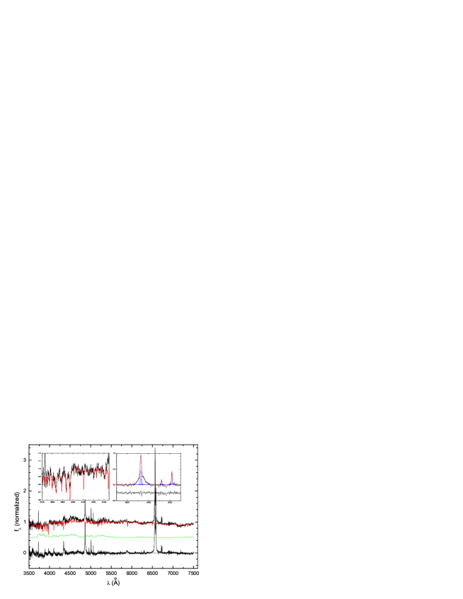
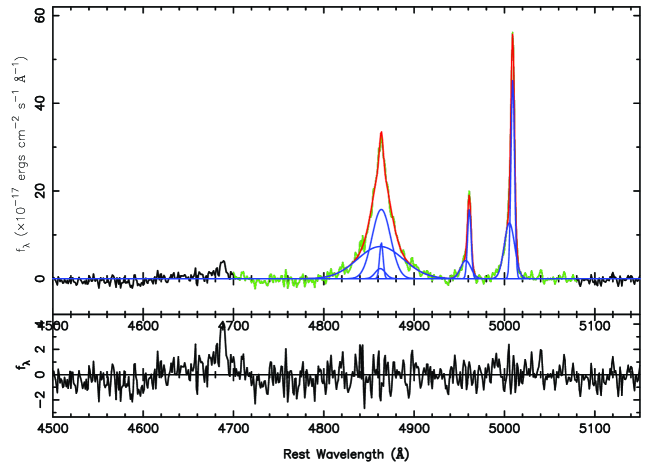
Figure 1: $Top$: An example fit for SDSS J123831.34+644356.5. The black line is the original spectrum after Galactic-extinction correction in the rest frame. The red line is the contribution from the host galaxy. The green line is the Fe ii emission. The residual is shown at the bottom. The left upper panel shows the region around Ca H+K $\lambda\lambda$ 3969, 3934 and G-band. In the right upper panel we show the H$\beta$ and [O iii] line fits, where the blue one with the highest peak is the IC, the blue one with the second highest peak is the BC, the two blue ones with the lower peaks are the components from NLRs. $Bottom$: An another example of line fit for SDSS J084716.88+334858.9. The black line is the original spectrum after Galactic-extinction correction, the starlight subtraction, and the Fe ii subtraction in the rest frame. The bottom panel is the residual. The multiple Gaussian components are in blue and the sum of them is in red. The fitting window is in green.

We use a largest sample of about 2000 NLS1s from SDSS DR3 (Zhou et al. 2006). Zhou et al. (2006) presented this sample of about 2000 NLS1s selected from objects assigned as ”QSOs” and ”galaxies” in the spectroscopic database of SDSS DR3. The only criterion is that the broad component of H$\beta$ or H$\alpha$ is detected and is narrower than 2200 km s^-1 in FWHM. Using a Lorentzian function to model the broad H$\beta$ profile, Zhou et al. (2006) obtained the FWHM and calculated SMBHs masses from the $R_{\rm BLR}-L_{5100}$ relation of Kaspi et al. (2000). We use the latest SDSS spectra from data release 6 (DR6).

We briefly outline our steps to do the SDSS spectral analysis. (1) We use simple stellar population (SSP) synthesis to model the stellar contribution in the Galactic extinction-corrected spectra in the rest frame (Cid Fernandes et al. 2005; Bian et al. 2007). We include 45 templates from Bruzual & Charlot (2003; BC03) and one power-law component (representing the AGN continuum emission). During the stellar population synthesis, we put twice the weight in the fit for strongest stellar absorption features, such as CaII K, G-band, and Ca II$\lambda\lambda$ 8498, 8542, 8662 triplet. For details, please see Bian et al. (2007) and the references therein. (2) The optical and ultraviolet Fe ii template from the prototype NLS1 I ZW 1 is used to subtract the Fe ii emission from the residual spectra after the above step. (3) Four Gaussians are used to model the H$\beta$ profile, and two sets of two Gaussians are used to model the [O iii] $\lambda\lambda 4959,5007$ lines. We take the same linewidth for each component, and fix the flux ratio of [O iii] $\lambda$4959 to [O iii] $\lambda$5007 to be 1:3. Two components of H$\beta$ (from the NLR) are set to have the same linewidth of each component of [O iii] $\lambda$5007 and their flux are constrained to be less than 1/2 of each component of [O iii] $\lambda 5007$. Two broad components are used to model broad H$\beta$ profile from the BLR contribution (broad component and intermediate component, BC and IC). We present our spectral fitting method in detail in Hu et al. (2008). In the above three steps, the best fit is reached by minimizing $\chi^{2}$, $\chi^{2}=\sum_{i}\left(\frac{y_{i}-y_{\rm model}}{\sigma_{i}}\right)^{2}/N$, where $\sigma_{i}$ is the error of the data set $(x_{i},y_{i})$, N is the degrees of freedom.

Objects without clear H$\beta$ or [O iii] lines are eliminated. In order to obtain a reliable spectral fit, we carefully select objects for analysis. We select objects by the following criteria: (1) the signal-to-noise ratio (S/N) is larger than 15. The S/N is measured in the wavelength 4800-5040Å, covering the range for line-fitting. (2) $\chi^{2}$ in above three steps (SSP, Fe ii subtraction, and H$\beta$ and [O iii] lines fitting) are less than 2.5. (3) the FWHM errors of BC and IC of H$\beta$ from BLR and [O iii] $\lambda\lambda 4959,5007$ are less than $100\%$. (4) The height of one component of [O iii] is less than the height of one component of [O iii] by 30%. The first criterion leads to about 900 NLS1s. The second and third criteria make sure we have a good fitting of H$\beta$ and [O iii] . The fourth criterion make us reliable to obtain the core/narrow component of [O iii] line, and their line width is used to trace the $\sigma_{*}$. Then we visually check these spectra one by one. In the end, we have a sample of 329 NLS1s.

The first moment of the line profile is

$$\lambda_{0}=\frac{\int\lambda P(\lambda)d\lambda}{\int P(\lambda)d\lambda},$$ (2)

The second moment of the line profile is

$$\sigma^{2}_{line}=\frac{\int\lambda^{2}P(\lambda)d\lambda}{\int P(\lambda)d\lambda}-\lambda_{0}^{2}.$$ (3)

We use the BC and IC to reconstruct the broad H$\beta$ profile as $P(\lambda)$. Then we use the method of Peterson et al. (2004) to measure the FWHM and $\sigma_{\rm H\beta}$ from the reconstructed broad H$\beta$ profile (Equations (2-3)). The error of $\sigma_{\rm H\beta}$ is calculated from the error of FWHM for BC and IC in the line fit. The FWHM measurement is not sensitive to the broad wing of H$\beta$, while the measurement of H$\beta$ second moment is. We have to make sure the necessary of using BC and IC in the H$\beta$ fitting (see also Dietrich et al. 2005). We use one broad component to model the H$\beta$ profile from the BLR at the same time. When the $\chi^{2}$ in the fitting is decreased by 20% with two-Gaussian respect to that with one-Gaussian, We have to make sure it is necessary to use BC and IC, and we use the result of two-Gaussian fitting, otherwise we use the result of one-Gaussian fitting. For H$\beta$ profile with one-Gaussian fitting, the second moment is directly from our fitting, not from Equations (2-3). For all objects, the measurement of FWHM is adopted from the two-Gaussian reconstructive profile. Hereafter, we call the total 329 NLS1s as sample A, 209 NLS1s with two-Gaussian fitting as sample B, and the other 120 NLS1s with one-Gaussian fitting as sample C.

As the strongest forbidden line in the SDSS spectral wavelength coverage, we use the gas velocity dispersion of the narrow/core [O iii] component from NLRs to trace $\sigma_{*}$, $\sigma^{core}_{\rm[OIII]}=\sqrt{\sigma_{\rm obs}^{2}-[\sigma_{\rm inst}/(1+z)]^{2}}$, where $z$ is the redshift. For SDSS spectra, the mean value of instrumental resolution $\sigma_{\rm inst}$ is 60 km s^-1  for [O iii] (e.g., Greene & Ho 2005a). We also reliably obtain $\sigma_{*}$ (correction the resolutions of the SDSS spectra and BC03 templates) from our SSP synthesis for about 98 NLS1s. The error of $\sigma_{*}$ is given by different typical errors for different effective S/Ns at 4020 Å (Bian et al. 2007).

3 Mass from $\sigma_{\rm H\beta}$ and FWHM

3.1 Mass estimation

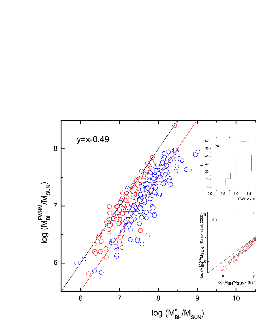
Figure 2: The mass from the H$\beta$ FWHM versus the mass from the H$\beta$ second moment. The blue circles denote objects in sample B where the H$\beta$ from BLRs can be fitted well by two-Gaussian with $\chi^{2}$ decreased by at least 20% with respect to that by one Gaussian. The red circles denote objects in sample C with the H$\beta$ from BLRs can be fitted well by one Gaussian in order to avoid the broad wing effect in measurement of the second moment. The solid line is 1:1, and the red line is the best linear fit with the fixed slope of 1 for sample B, y=x-0.49. Then FWHM and $\sigma_{\rm H\beta}$ are measured from the reconstructed broad H$\beta$ profile. For sample C, there is a scatter from 1:1. For sample C, mass from $\sigma_{\rm line}$ can be increased by 0.13 dex with respect to that from FWHM. (a) The distribution of $\rm FWHM/\sigma(H\beta)$ for 209 NLS1s in sample B. (b) SMBH mass from Zhou et al. (2006) versus that with updated the $R_{\rm BLR}-L_{5100}$ relation of Bentz et al. (2006).

With our measurement of $\sigma_{\rm H\beta}$, we use the more recent $R_{\rm BLR}-L_{5100}$ relation (which seems to hold for NLS1s; Peterson et al. 2004) of Bentz et al. (2006) and $f=3.85$ (Collin et al. 2006) to calculate the SMBHs masses in NLS1s. We also calculate the mass from our FWHM for the H$\beta$ profile from the BLR by $R_{\rm BLR}-L_{5100}$ relation of Bentz et al. (2006) and $f=3$ (Netzer 1990). In Figure 2, we compare these two masses. For sample B, the best linear fit with fixed slope of 1 gives y=x-0.49, the mass from $\sigma_{\rm H\beta}$ is on average larger by 0.49 dex than that from FWHM. In Figure 2a, we show the distribution of $\rm FWHM/\sigma$, $1.33\pm 0.36$, which deviates from 2.35 for a Gaussian profile. Our mass correction from $\sigma_{\rm H\beta}$ respective to mass from FWHM is mainly due to the H$\beta$ emission-line profile deviation from the Gaussian profile. For six NLS1s in Peterson et al. (2004), we find that the mass based on $\sigma_{\rm H\beta}$ is on average larger by 0.46 dex with respect to that from FWHM, which is consistent with our calculation.

By using the FWHM derived from the Lorentzian profile, Zhou et al. (2006) calculated SMBHs masses from the $R_{\rm BLR}-L_{5100}$ relation of Kaspi et al. (2000, $R_{\rm BLR}\propto L_{5100}^{0.7}$) and $f=3$. For comparison with the results of Zhou et al. (2006), we use the updated $R_{\rm BLR}-L_{5100}$ relation of Bentz et al. (2006, $R_{\rm BLR}\propto L_{5100}^{0.518}$) and $f=3$ to calculate the mass. For the FWHM from Zhou et al. (2006), the updated $R_{\rm BLR}-L_{5100}$ relation of Bentz et al. (2006) would lead the masses of Zhou et al. (2006) to be larger by 0.1-0.3 dex for NLS1s with mass less than $10^{7}M_{\odot}$ (see Figure 2b). By the best linear fit through zero, we find FWHM in Zhou et al. (2006) derived from the Lorentzian profile is $0.84\pm 0.01$ of our FWHM for objects in sample B, which leads to the SMBH mass decreasing by 0.15 dex if we use the FWHM of Zhou et al. (2006).

The usa of $R_{\rm BLR}-L_{5100}$ relation of Kaspi et al. (2005) will decrease $M_{\rm BH}$ by 0.17 dex with respect to that of Kaspi et al. (2000). If we use $f=3.85$ instead of $3$, the mass will increase by 0.11 dex. The uncertainty of the mass calculation from the H$\beta$ line is mainly from the systematic uncertainties, up to about 0.5 dex, which is due to the unknown kinematics and geometry in BLRs, and perhaps the effects of radiation pressure (e.g., Krolik 2001; Peterson et al. 2004; Decarli et al. 2008; Marconi et al. 2008).

3.2 The $M_{\rm BH}-\sigma^{\rm core}_{\rm[O~{}III]}$ relation

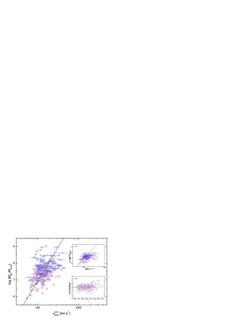
Figure 3: The SMBH mass versus the core/narrow [O iii] gas velocity dispersion. The mass is derived from the H$\beta$ second moment. The sybols are same as Figure 2. The solid line is the $M_{\rm BH}-\sigma_{*}$ relation of Tremaine et al. (2002). The green dashed line is the $M_{\rm BH}-\sigma_{*}$ relation of Ferrarese & Ford (2005). (a) SMBH mass from H$\beta$ FWHM versus the [O iii] gas velocity dispersion. (b) Mass deviation versus the redshift. The solid line is the relation of Woo et al. (2008).

In Figure 3, we show the SMBH mass from $\sigma_{\rm H\beta}$ versus $\sigma_{\rm[OIII]}^{core}$. In Figure 3a, we show the mass derived from our FWHM versus $\sigma_{\rm[OIII]}^{core}$. It is obvious that the mass from FWHM deviates from Tremaine et al. relation (solid line in Figure 3a), which is consistent with the result of Zhou et al. (2006). In Figure 3a, we show the SMBH mass from $\sigma_{\rm H\beta}$ versus that from our FWHM. The SMBH masses based on $\sigma_{\rm H\beta}$ in 209 NLS1s of sample B is larger by about 0.5 dex with respect to that from FWHM.

For the solid line in Figure 3, the $M_{\rm BH}-\sigma_{*}$ relation, $M_{\rm BH}(\sigma_{*})=10^{8.13}[\sigma_{*}/(200\ \rm kms^{-1})]^{4.02}~{}~{}M_{\odot}$ (Tremaine et al. 2002), we calculate the deviation of mass (see Table 1). In Figure 3b, we show the mass deviation from the Tremaine et al. relation versus the redshift. The dashed line is for no deviation, and the solid line is the relation found by Woo et al. (2008). For redshifts of NLS1s larger than 0.4, their mean mass deviation is $0.28\pm 0.82$ respect to Tremaine et al. relation, and for NLS1s with redshift less than 0.4, the mean mass deviation is $-0.04\pm 0.58$ (Woo et al. 2008). We calculate the Eddington ratio, i.e., the ratio of the bolometric luminosity ($L_{\rm bol}$) to the Eddington luminosity ($L_{\rm Edd}$), where $L_{\rm Edd}=1.26\times 10^{38}(M_{\rm BH}/M_{\odot}){\rm erg\ s}^{-1}$. The bolometric luminosity is calculated from the monochromatic luminosity at 5100Å , $L_{\rm bol}=c_{\rm B}\lambda L_{\lambda}(5100\AA)$, where we adopt the correction factor $c_{\rm B}$ of 9 (Kaspi et al. 2000; Richards et al. 2006; Netzer & Trakhtenbrot 2007). We do not find larger mass deviations for objects with larger Eddington ratio. In Table 1, we give the mass, Eddington ratio, and the mass deviation from the $M_{\rm BH}-\sigma_{*}$ relation for A, B, C samples. For sample B, mass from $\sigma_{\rm H\beta}$ can be increased by $\sim$ 0.5 dex with respect to that from FWHM. For sample C, mass from $\sigma_{\rm line}$ can be increased by 0.13 dex with respect to that from FWHM, which is due to the values of $f$ that we are using for sigma ($f=3.85$) and FWHM/2 ($f=3$) are not exactly consistent with a single Gaussian, whereas in order to get the same mass for a single Gaussian the ratio of f values is 1.38. We also notice that, for NLS1s with mass larger than $10^{8}M_{\odot}$, they tend to fall above the Tremaine et al. relation.

Table 1: The SMBH masses from the $\sigma_{\rm H\beta}$ and FWHM.

	A	B	C
log $M_{\rm BH}^{\sigma}$	$7.53\pm 0.50$	$7.69\pm 0.48$	$7.25\pm 0.40$
$L_{\rm bol}/L_{\rm Edd}(\sigma)$	$-0.81\pm 0.28$	$-0.84\pm 0.27$	$-0.75\pm 0.28$
$\Delta{\rm log}M_{\rm BH}^{\sigma}$	$0.03\pm 0.65$	$0.12\pm 0.68$	$-0.13\pm 0.55$
log $M_{\rm BH}^{\rm FWHM}$	$7.17\pm 0.44$	$7.20\pm 0.44$	$7.12\pm 0.43$
$L_{\rm bol}/L_{\rm Edd}(\rm FWHM)$	$-0.44\pm 0.37$	$-0.35\pm 0.37$	$-0.61\pm 0.31$
$\Delta{\rm log}M_{\rm BH}^{\rm FWHM}$	$-0.34\pm 0.65$	$-0.38\pm 0.70$	$-0.26\pm 0.57$

†: A: for total 329 NLS1s; B: for 209 NLS1s in sample B; C: for 120 NLS1s in sample C. The mass deviation is based on Tremaine et al.’s relation when $\sigma_{\rm[OIII]}^{core}$ is used for $\sigma_{*}$.

4 Discussion

4.1 Large SMBH masses in NLS1s?

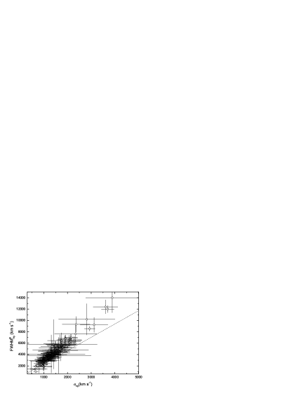
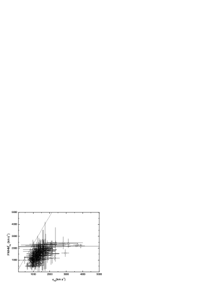
Figure 4: The FWHM of BC ($top$) and IC ($bottom$) versus the H$\beta$ second moment for sample B of 209 NLS1s. The dashed line is the relation between FWHM and the second moment, $\rm FWHM=\sigma_{\rm H\beta}\times 2.35$, for a Gaussian line profile.

In Figure 3, we find that, for some NLS1s, mass from $\sigma_{\rm H\beta}$ is very large, up to $10^{8}-10^{9}M_{\odot}$, which is due to their obvious broad wings in their H$\beta$ profiles. With the near-IR imaging data, Ryan et al. (2007) found that the average SMBH mass in their NLS1s sample is $10^{7.9}M_{\odot}$, where the mass is calculated from the mass and host galaxy luminosity relation. The mass is typical for broad line Seyfert 1 galaxies. They find that it is larger by 1.5 dex respect to the mass calculated from the FWHM of Veron-Cetty et al. (2001). We note that these objects have broad wings in their H$\beta$ profile, especially in their H$\alpha$ profile (Figure 2 in Veron-Cetty et al. 2001). It is possible that the sample of Zhou et al. (2006) have some objects that should not be classified as NLS1s. Considering the effects of the random velocity and the inclination in SMBH mass estimation of NLS1s, Decarli et al. (2008) find that these effects would increase the mass for NLS1s by 0.84 dex, which can account for the mass difference between NLS1s and BLS1s. The definition of NLS1s need to be reexamined if we think that NLS1s harbor rapid growing small SMBH with high accretion rate.

4.2 $\sigma_{\rm H\beta}$ and FWHMs of BC, IC

The flux ratio of H$\beta$ to [O iii] $\lambda$5007 from NLRs is often taken to be around 10% (e.g. Osterbrock & Pogge 1985; McGill et al. 2008). Rodriguez-Ardila et al. (2000) suggested this ratio is about 20%-100%, this high value due to that they just used two-Gaussian to model the total H$\beta$ profile and assumed the narrow H$\beta$ component is from NLRs. The flux ratio of H$\beta$ to [O iii] $\lambda$5007 from NLRs depend on the physics of the low-density gas found in NLRs photoionized by AGN, which is beyond the scope of this paper (e.g. Groves et al. 2006; Kewley et al. 2006). During our fitting procedure of the H$\beta$ and [O iii] lines, we add a conservative constraint to the H$\beta$ contribution from NLRs, less than a half of [O iii] $\lambda$5007 flux.

For 209 NLS1s in sample B, the second moment $\sigma_{\rm H\beta}$ is calculated from the reconstructed H$\beta$ profiles from BC and IC. We did a comparison between $\sigma_{\rm H\beta}$ and the FWHM of IC/BC. In Figure 4, we show $\sigma_{\rm H\beta}$ versus FWHM of IC and BC. The dashed line is the relation of $\rm FWHM=2.35\times\sigma$ when a Gaussian profile is measured. We find that there is a much stronger correlation between the $\sigma_{\rm H\beta}$ versus FWHM of BC with respect to that for IC (see Figure 4). If using the $\sigma_{\rm H\beta}$ to calculate the SMBHs masses, the result depends much more on the BC FWHM, and less on the narrower IC FWHM. We think that if the H$\beta$ profile from BLRs can be fitted well by one Gaussian, for mass, there is no difference for the usage of H$\beta$ FWHM and the $\sigma_{\rm H\beta}$.

The existence of BC and IC in the H$\beta$ profile from BLRs have been investigated by many people (Baldwin et al. 1998; Wills et al., 1993; Brotherton et al. 1994; Rodriguez-Ardila et al. 2000; Leighly 2004; Dietrich et al. 2005), and it is suggested that BC and IC are emitted from two distinct emission region. For 12 NLS1s, Dietrich et al. (2005) found that $\rm FWHM_{BC}=3275\pm 800{\rm km\ s}^{-1}$ and $\rm FWHM_{IC}=1200\pm 300{\rm km\ s}^{-1}$. For our 209 NLS1s in sample B, we also found that $\rm FWHM_{BC}=4098\pm 1751{\rm km\ s}^{-1}$ and $\rm FWHM_{IC}=1385\pm 492{\rm km\ s}^{-1}$. Therefore, it is clear that there exists a BC in NLS1s that are typical for BLS1s, and the IC displays typical H$\beta$ FWHM in NLS1s. The equivalent width (EW) of BC for our 209 NLS1s in sample B is $19.4\pm 8.6$Å  and $16.1\pm 8.0$Å for IC EW. There is no correlation between them.

4.3 $M_{\rm BH}-\sigma_{*}$ relation

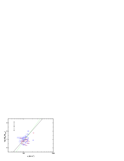
Figure 5: The $M_{\rm BH}-\sigma_{*}$ relation for 37 AGNs with reliable measurements of $\sigma_{*}$. The blue and red circles have the same meaning as in Figure 2. The solid line is the $M_{\rm BH}-\sigma_{*}$ relation of Tremaine et al. (2002). The Green dashed line is the $M_{\rm BH}-\sigma_{*}$ relation of Ferrarese & Ford (2005). The line in the left corner denotes the typical error in mass calculation.

With FWHM from the H$\beta$ Lorentzian profile, Zhou et al. (2006) use the $R_{\rm BLR}-L_{5100}$ relation of Kaspi et al. (2000) and $f=3$ to calculate the mass. The updated $R_{\rm BLR}-L_{5100}$ relation of Bentz et al. (2006) would lead to the mass of Zhou et al. (2006) larger by 0.1-0.3 dex for NLS1s with mass less than $10^{7}M_{\odot}$ (see Figure 2b), which would place NLS1S close to the Tremaine et al. $M_{\rm BH}-\sigma_{*}$ relation when $\sigma_{*}$ is adopted from $\sigma_{\rm[NII]}$ (see Figure 29 in Zhou et al. 2006). For a sample of 58 NLS1s selected from 11th edition of the ”Catalogue of Quasars and AGNs ” (Veron-Cetty & Veron 2003) and SDSS DR3, by the $R_{\rm BLR}-L_{5100}$ relation of Kaspi et al. (2005), Komossa & Xu (2007) suggested that NLS1s do follow the $M_{\rm BH}-\sigma_{*}$ relation found in inactive galaxies after excluding ”blue outliers” (see Bian & Zhao 2005).

Using the second moment of broad H$\beta$ profile, we find that the SMBH mass would be larger by $\sim$ 0.5 dex with respect to that from H$\beta$ FWHM in sample B with necessary two-Gaussian fitting. The larger masses make NLS1s follow the Tremaine et al. relation when the $\sigma_{\rm[OIII]}^{core}$ is used as a surrogate for the bulge velocity dispersion. In Figure 3, we find that some AGN lie far below the $M_{\rm BH}-\sigma_{*}$ relation and we tried to determine if they are ”blue outliers”. No ”blue outliers” are found or it is impossible to measured the [O iii] blueshift due to the low S/N in [S ii] or [O ii] . We also use the [N ii] FWHM (Zhou et al. 2006) as the $\sigma_{*}$, and find as similar result to that shown in Figure 3, but with more scatter. The [N ii] FWHM measurement depends on the H$\alpha$ profile fitting. And the [N ii] FWHM is consistent with FWHM of [O iii] core component, although the correlation is very weak (Komossa & Xu 2007).

In Figure 5, we plot $M_{\rm BH}$ from $\sigma_{\rm H\beta}$ versus $\sigma_{*}$ for 37 NLS1s. For the $\sigma_{*}$ from SSP synthesis, its uncertainty based on effective S/N at 4020Å is typically about: 24 km s^-1 at S/N=5; 12 km s^-1 at S/N=10; 8 km s^-1 at S/N=15, where the effective S/N is the S/N (measured between 4010 and 4060 Å) multiplied by the stellar fraction (Cid Fernandes et al. 2005; Bian et al. 2007). The mass is calculated for AGNs that satisfy the first two criteria in section 2. The blue circles denote AGN with necessary two-Gaussian fits and the red circles denote AGN with one-Gaussian fits, which is the same as that in Figure 2. For the total 37 NLS1s in Figure 5, the mass is between $10^{6}-10^{8}M_{\odot}$, and the distribution of the mass deviation is $-0.24\pm 0.46$. For 14 AGN with two-Gaussian fits, the distribution of the mass deviation is $-0.14\pm 0.50$, and for 23 AGN with one-Gaussian, the distribution of the mass deviation is $-0.29\pm 0.43$. If these 23 NLS1s follow Tremaine et al. relation, we need $f=7.7$. The $\sigma^{core}_{\rm[OIII]}$ is slightly larger than $\sigma_{*}$ for these 37 NLS1s (see Botte et al. 2005). For about 3000 Seyfert 2 galaxies, Zhou et al. (2006) also found that $\sigma_{\rm[NII]}=\sigma_{*}\times(2.62/2.35)$ and overestimate the $\sigma_{*}$ (also see Onken et al. 2004). Therefore, using the gas velocity dispersion to trace $\sigma_{*}$ will place NLS1s close to the $M_{\rm BH}-\sigma_{*}$ relation and make the mass deviation smaller by 0.19 dex.

For the total 37 NLS1s, there exists marginal evidence that they deviate from the $M_{\rm BH}-\sigma_{*}$ relation found in inactive galaxies. For 23 NLS1s with mass lower than $10^{7}M_{\odot}$, the deviation becomes much larger, up to $-0.46\pm 0.40$ (also see Figure 3), which is consistent with the result of Botte et al. (2005, their figure 3), although it is not the case for the sample of Greene & Ho (2006) (also see Barth et al. 2005). If these 23 NLS1s follow the Tremaine et al. relation, we need $f=11.1$. It is possible that the sample of Zhou et al. (2006) have some objects that can’t be classified by NLS1s. It is possible that there exists true NLS1s with rapid growing small SMBH. The reliable measurements of mass and the $\sigma_{*}$ are important for this kind of work.

5 conclusions

The second moment of H$\beta$ line from BLRs is calculated to derive the SMBHs masses for a sample of 329 NLS1s selected from SDSS. The main conclusions can be summarized as follows: (1) For objects with necessary two-Gaussian fitting, the mean value of SMBH masses from the H$\beta$ second moment is larger by about 0.5 dex with respect to that from the H$\beta$ FWHM. (2) Using the narrow/core [O iii] gas velocity dispersion as a surrogate for the stellar velocity dispersion, we find the new masses based on the H$\beta$ broad emission line second moment bring them to the Tremaine et al. relation; (3) The H$\beta$ second moment is more strongly correlated with the BC FWHM rather than the IC FWHM. (4) Using the $\sigma_{*}$ measured from SSP synthesis, we find that, for NLS1s with masses lower than $10^{7}M_{\odot}$, they are marginally below the Tremaine et al. relation considering the larger scatter in mass calculation. If these 23 NLS1s follow Tremaine’s relation, we need $f=11.1$.

References

- [] Adelman-McCarthy, J., et al. 2007, ApJS, 172, 634
- [] Baldwin, J. A., et al., 1988, ApJ,327, 103
- [] Barth, A. J., et al., 2005, ApJ, 619, L151
- [] Bentz, M. C., et al. 2006, ApJ, 644, 133
- [] Bian, W. H., Zhao, Y. H. 2004, MNRAS, 347, 607
- [] Bian, W. H., Yuan, Q. R., & Zhao, Y. H. 2005, MNRAS, 364, 187
- [] Bian, W. H., Yuan, Q. R., & Zhao, Y. H. 2006, MNRAS, 367, 860
- [] Bian, W. H., Chen, Y. M., Gu Q. S., Wang, J. M. 2007, ApJ, 668, 721
- [] Boller, Th., Brandt, W. N., Fink, H., 1996, A& A, 305 , 53
- [] Botte, V., et al. 2005, MNRAS, 356, 789
- [] Brotherton, M. S., et al., 1994, ApJ, 423, 131
- [] Cid Fernandes, R., Mateus, A., Sodre L., Stasinska, G., Gomes J. 2005, MNRAS, 358, 363
- [] Collin, S. et al. 2006, A&A, 456, 75
- [] Decarli R., et al., 2008, MNRAS, astro-ph/0801.4560
- [] Dietrich, M., Crenshaw, D. M., & Kraemer, S. B., 2005, ApJ, 623, 700
- [] Ferrarese, L., & Ford, H. 2005, Space Sci. Rev., 116, 523
- [] Ferrarese, L., Merritt D., 2000, ApJ, 539, L9
- [] Fromerth, M. J., & Melia, F. 2000, ApJ, 533, 172
- [] Gebhardt K., et al., 2000, ApJ, 539, L13
- [] Gebhardt, K., et al. 2000, ApJ, 539, L13
- [] Greene, J. E., Ho, L. C. 2005a, ApJ, 627, 721
- [] Greene, J. E., Ho, L. C. 2005b, ApJ, 630, 122
- [] Greene, J. E., Ho, L. C. 2006, ApJ, 641, L21
- [] Grupe, D., & Mathur, S. 2004, ApJ, 606, L41
- [] Groves B. A., Heckman T. M. & Kaufmann G. 2006, MNRAS, 371, 1559
- [] Hu, C., et a., 2008, ApJ, in press, astro-ph/0807.2059
- [] Kaspi, S., Maoz, D., Netzer, H., Peterson, B.M., Vestergaard M., Jannuzi B.T., 2005, ApJ, 629, 61
- [] Kaspi, S., Smith, P.S., Netzer, H., Maoz, D., ,Jannuzi, B.T., Giveon U., 2000, ApJ, 533, 631
- [] Kewley L. J., et al. 2006, MNRAS, 372, 961
- [] Komossa, S. & Xu, D. W., 2007, ApJ, 667, L33
- [] Krolik, J. H., 2001, ApJ, 551, 72
- [] Leighly, K. M., 2004, ApJ, 611, 125
- [] Marconi A., et al., 2008, ApJ, astro-ph/0802.2021
- [] Mathur, S., Kuraszkiewicz, J., Czerny, B. 2001, NewA, 6, 321
- [] Mullaney, J. R., & Ward, M. J., 2008, MNRAS, 385, 53
- [] McGill, K. L. et al., 2008, ApJ, 673, 703
- [] McLure, R. J., & Jarvis, M. J. 2004, MNRAS, 353, L45
- [] Nelson, C. H., 2001, ApJ, 544, L91
- [] Netzer H., Trakhtenbrot B. 2007, ApJ, 654, 754
- [] Onken, C. A., et al. 2004, ApJ, 615, 645
- [] Osterbrock, D., & Pogge, R. W., 1985, ApJ, 297, 116
- [] Netzer, H. 1990, in Active Galactic Nuclei, ed. R. D. Blandford, H. Netzer, & L. Woltjer (Berlin: Springer), 137
- [] Peterson, B. M., ApJ, 2004, 613, 682
- [] Rees, M. J. 1984, ARA&A, 22, 471
- [] Richards, G. T., et al., 2006, ApJS, 166, 470
- [] Rodriguez-Ardila, A., et al., 2000, ApJ, 538, 581
- [] Ryan, C. J., Robertis, M.M.D., Virani, S., Laor, A., Watson, P. c., 2007, ApJ, 654, 799
- [] Salviander, S., et al. 2007, ApJ, 622, 131
- [] Shen, J.J. et al., AJ, 135, 928
- [] Tremaine, S., et al. 2002, Ap J, 574, 740
- [] Veron-Cetty, M.-P., Veron, P., & Goncalves, A. C. 2001, A&A, 372, 730
- [] Veron-Cetty, M.-P., & Veron, P. 2003, A&A, 412, 399
- [] Vestergaard, M., & Peterson, B. M., 2006, ApJ, 641, 689
- [] Watson, P. C., Grupe, D., Mathur, S. 2007, AJ, 133, 2435
- [] Wills, et al., 2003,ApJ, 415, 563
- [] Woo, J. H. et al., 2008, ApJ, in press, astro-ph/0804.0235
- [] Zhou, H. Y., et al. 2006, ApJS, 166, 128