SNUST 080801

Integrable Spin Chain

of

Superconformal U$(M)\times\overline{{\rm U}(N)}$ Chern-Simons Theory

Dongsu Bak^a,     Dongmin Gang^b,     Soo-Jong Rey^b

^a Physics Department, University of Seoul, Seoul 130-743 KOREA

^b School of Physics & Astronomy, Seoul National University, Seoul 151-747 KOREA

dsbak@uos.ac.kr     arima275@snu.ac.kr     sjrey@snu.ac.kr

ABSTRACT

${\cal N}=6$ superconformal Chern-Simons theory with gauge group U$(M)\times\overline{{\rm U}(N)}$ is dual to $N$ M2-branes and $(M-N)$ fractional M2-branes, equivalently, discrete 3-form holonomy at $\mathbb{C}^{4}/\mathbb{Z}_{k}$ orbifold singularity. We show that, much like its regular counterpart of $M=N$, the theory at planar limit have integrability structure in the conformal dimension spectrum of single trace operators. We first revisit the Yang-Baxter equation for a spin chain system associated with the single trace operators. We show that the integrability by itself does not preclude parity symmetry breaking. We construct two-parameter family of parity non-invariant, alternating spin chain Hamiltonian involving three-site interactions between ${\bf 4}$ and $\overline{\bf 4}$ of SU(4)_R. At weak ‘t Hooft coupling, we study the Chern-Simons theory perturbatively and calculate anomalous dimension of single trace operators up to two loops. The computation is essentially parallel to the regular case $M=N$. We find that resulting spin chain Hamiltonian matches with the Hamiltonian derived from Yang-Baxter equation, but to the one preserving parity symmetry. We give several intuitive explanations why the parity symmetry breaking is not detected in the Chern-Simons spin chain Hamiltonian at perturbative level. We suggest that open spin chain, associated with open string excitations on giant gravitons or dibaryons, can detect discrete flat holonomy and hence parity symmetry breaking through boundary field.

1 Introduction

In continuation of remarkable development by Aharony, Bergman, Jafferis and Maldacena (ABJM) [1], Aharony, Bergman and Jafferis (ABJ) [2] identified further examples of AdS/CFT correspondences: three-dimensional ${\cal N}=6$ superconformal Chern-Simons theory with gauge group U(M)${}_{k}\times\overline{\rm U(N)}_{-k}$, where $k$ denotes the Chern-Simons level, is dual to Type IIA string theory on AdS${}_{4}\times\mathbb{CP}^{3}$ [3] with $B_{\rm NS}$ holonomy turned on over $\mathbb{CP}_{1}\subset\mathbb{CP}_{3}$. For consistency with flux quantization of Ramond-Ramond field strengths, the $B_{\rm NS}$ holonomy is not arbitrary but takes a value in $\mathbb{Z}_{k}$ (measured in string unit). From M-theory viewpoint, the gravity dual background descends from AdS${}_{4}\times\mathbb{S}^{7}/\mathbb{Z}_{k}$ once M-theoretic discrete torsion is turned on over a torsion 3-cycle in $\mathbb{S}^{7}/\mathbb{Z}_{k}$. The corresponding torsion flux takes a value in $H^{4}(\mathbb{S}^{7}/\mathbb{Z}_{k},\mathbb{Z})=\mathbb{Z}_{k}$. In the limit $M\rightarrow N$, these discrete fluxes are turned off and the new correspondence [2] is reduced to the correspondence identified earlier [1] .

The purpose of this paper is to show that, much the same as the ABJM theory [5, 6], the ABJ theory also exhibits integrability structure in the spectrum of anomalous dimensions for single trace local operator . By extending the computations of [6], we shall find that the spin chain Hamiltonian that governs two-loop operator mixing and anomalous dimensions in ABJ theory is essentially the same as that of ABJM theory modulo suitable change of perturbative coupling parameters.

We organized this paper as follows. In section 2, in comparison with the ABJM theory, we list several new features of the ABJ theory that will be directly relevant for the quest of integrability structure. In section 3, we revisit the derivation of integrable spin chain from Yang-Baxter equations. We emphasize that parity symmetry of the spin chain is broken in general. We construct the most general parity non-invariant, integrable spin chain Hamiltonian and show that, up to overall scaling, there are two-parameter family of Hamiltonian. In section 4, we compute operator mixing and anomalous dimensions of single trace operators at two loops. We find that the resulting Chern-Simons spin chain Hamiltonian coincides with the spin chain Hamiltonian derived from Yang-Baxter equation. In fact, the Hamiltonian is exactly the same as the Hamiltonian for ABJM theory [5, 6], except that the coupling parameter $N^{2}$ in the ABJM theory is now replaced by $MN$. In section 5, we offer several arguments why the spin chain Hamiltonian does not detect parity violation effect of the $B_{\rm NS}$ holonomy and illustrate them by studying giant magnon. We also suggest that the discrete holonomy may be visible for an open spin chain associated with open string attached to giant graviton or dibaryon operators.

2 Aspects of ABJ Theory

In the ABJ theory, since the number of fractional branes is a new parameter added to the ABJM theory, there are three coupling parameters, $M,N,k$. In contrast to ${\cal N}=4$ super Yang-Mills theory, a unique feature of the ABJ theory (as well as ABJM theory) is that the coupling parameters are all integer-valued. In this section, we elaborate several notable aspects of the ABJ theory that will become relevant for later investigation of integrability. For these, we shall take the generalized ‘t Hooft planar limit (in the convention $M\geq N$):

$$M,\,\,\,N,\,\,\,k\longrightarrow\infty\qquad\mbox{with}\qquad\lambda\equiv{N\over k},\quad\overline{\lambda}\equiv{M\over k},\quad b\equiv{(M-N)\over k}\quad\mbox{fixed}\,,$$ (2.1)

though some of the results are extendible beyond this limit. Among these, the parameter $b$ is parity-odd and measures parity symmetry breaking effects in ABJ theory.

In this section, we elaborate several salient features of the ABJ theory that will become directly relevant for our foregoing investigation on integrability structure.

• From the viewpoint of M2-branes probing $\mathbb{C}^{4}/\mathbb{Z}_{k}$ orbifold singularity, the ABJ theories arise when, in addition to $N$ M2-branes, $(M-N)$ fractional M2-branes are localized at the orbifold singularity. In the much studied situation of $N$ D3-branes probing ${\cal M}_{5}/\Gamma$ orbifold singularity, adding fractional D-branes [9, 10] at the orbifold singularity [11, 12] led to running of otherwise constant gauge coupling parameter and hence to loss of the conformal invariance. This implies that, in the large $N$ limit, gravity dual background is deformed away from AdS${}_{5}\times{\cal M}_{5}/\Gamma$ [13, 14]. In the ABJ theories, even though fractional M2-branes are introduced, the supergravity background is not deformed at all and retains AdS${}_{4}\times\mathbb{S}^{7}/\mathbb{Z}_{k}$. We can understand this curious feature from noting that the gauge-gravity correspondence at hand involves superconformal Chern-Simons theories. In the latter theories, coupling parameters $M,N,k$ are all quantized to integer values. Therefore, at quantum level, these coupling parameters cannot possibly run under renormalization group flow. As such, we expect that operator mixing and anomalous dimensions of gauge invariant composite operators are still organized in the planar limit $M,N\rightarrow\infty$ as an analytic perturbative series expansion of the ‘t Hooft coupling parameters (2.1) within finite radius of convergence .

• Introducing fractional M2-branes or turning on $B_{\rm NS}$ holonomy, the parity symmetry is broken in the supergravity dual background and, in accordance with AdS/CFT correspondence, in the superconformal Chern-Simons theory. Apparently, parity transformation maps the Chern-Simons parameters by $k$ to $-k$ while holding $M,N$ fixed. In the planar limit (2.1), this maps $b$ to $-b$ while holding $\lambda,\overline{\lambda}$ fixed. We recall that the parity symmetry $P$ in ABJM theory was defined as, under $x^{m}\rightarrow-x^{m}$,

  $$P:\hskip 28.45274pt(A_{m},\overline{A}_{m},Y^{I},Y^{\dagger}_{I})\qquad\rightarrow\qquad(-\overline{A}_{m},-A_{m},Y^{\dagger}_{I},Y^{I}).$$ (2.2)

  In particular, since $Y^{I}\leftrightarrow Y^{\dagger}_{I}$, the parity exchanges the two isomorphic gauge groups, U(N) and $\overline{\rm U(N)}$. In the corresponding spin chain, this was identified with interchange of two interlaced chains of ${\bf 4}$’s and $\overline{\bf 4}$’s. From the viewpoint of SU(4) symmetry, this is equivalent to charge conjugation. As such, the above $(2+1)$-dimensional parity transformation acts on the spin chain as $(1+1)$-dimensional parity transformation:

  $$P:\hskip 28.45274pt\mbox{Tr}(Y^{I_{1}}Y^{\dagger}_{J_{1}}\cdots Y^{I_{n}}Y^{\dagger}_{J_{n}})\qquad\rightarrow\qquad\mbox{Tr}(Y^{J_{n}}Y^{\dagger}_{I_{n}}\cdots Y^{J_{1}}Y^{\dagger}_{I_{1}}).$$ (2.3)

  Hence, under this generalized parity transformation, the ABJM theory and the corresponding spin chain were manifestly invariant. Now, in the ABJ theory, the above parity transformation cannot possibly be a symmetry since, among others, the two gauge groups are different and cannot be exchanged. In fact, as we shall see below, the parity maps one ABJ theory with a given gauge group to another with different gauge group. Therefore, the newly identified correspondences of the ABJ theoy offer an excellent playground for exploring physics associated with parity symmetry and its breaking. In the quest of the integrability, this also raises very interesting issues: Is integrability compatible with parity symmetry breaking? Is parity symmetry breaking always reflected in the associated spin chain system? If so, what kind of spin chain Hamiltonian and higher conserved charges does it lead to? How visible is the parity symmetry breaking effect at weak and strong ‘t Hooft coupling regimes?

  In the ABJM theory, the parity transformation mapped the theory to itself, viz. parity invariant. In ABJ theory, the parity transformation relates one theory to another in a rich manner. To see this, recall that the ABJ theory with U(M)${}_{k}\times\overline{\rm U(N)}_{-k}$ gauge group is realizable via regular and fractional D3-branes threading between two diametrically separated $(p,q)$-branes of charge $(1,0)\oplus(1,k)$. If we adiabatically move $(1,0)$-brane and $(1,k)$-brane relatively and exchange their locations, the $(M-N)$ fractional D3-branes will disappear on one interval of the two $(p,q)$-branes and the $k-(M-N)$ fractional D3-branes are created on the other interval [16, 17]. Therefore, the original D3-branes $M_{k}\oplus N_{-k}$ is transformed to the one $N_{k}\oplus(N+k-(M-N))_{-k}$. Combining also with the parity transformed theory, we then have equivalence relations:

  $${\rm U(M)}_{k}\times\overline{{\rm U(N)}}_{-k}\,\,\,\simeq\,\,\,{\rm U(N)}_{k}\times\overline{{\rm U}(2N-M+k)}_{-k}\,\,\,\simeq\,\,\,{\rm U}(N)_{k}\times\overline{{\rm U}(M)}_{-k}.$$ (2.4)

  Notice that the relation is entirely among Chern-Simons theories. In particular, the middle theory is always strongly coupled, since the ‘t Hooft coupling of the second gauge group is always great than unity. This is exciting; in the quest of integrability and its interpolation between weak and strong coupling limits, the above equivalence relations may provide a new useful trick to extract physical observables such as (generalized) scaling functions not just at weak and strong ‘t Hooft coupling limits but also at ${\cal O}(1)$ regimes (albeit the drawback that these are all in lower-dimensional field theories).

• The number of fractional M2-branes is not arbitrary but is limited to $0\leq(M-N)\leq k$. This is most clearly seen from decoupling limit of $(M-N)$ many fractional M2-branes from $N$ many regular M2-branes. Low-energy dynamics of the fractional brane is described by ${\cal N}=3$ supersymmetric pure Chern-Simons theory with gauge group U$(M-N)_{k}$. Quantum mechanically, the Chern-Simons level $k$ of this theory ought to remain the same. This can be understood, for example, from the brane construction mentioned above: at all scales of D3-brane dynamics, the $(p,q)$-brane charges are held fixed. But such a non-renormalization property turns out possible only if $(M-N)\leq k$. To see this, we can sequentially integrate out superpartners of the gauge fields first and then the gauge field. The first step yields a bosonic pure Chern-Simons theory with gauge group U$(M-N)_{k^{\prime}}$ where $k^{\prime}=k-(M-N)\mbox{sign}(k)$. The second step shifts the Chern-Simons level further to $k^{\prime\prime}=k^{\prime}+(M-N)\mbox{sign}(k^{\prime})$. We see that the Chern-Simons level at quantum level $k^{\prime\prime}$ remains the same as the classical one $k$ if and only if $(M-N)\leq k$. Stated in the planar limit (2.1), this quantum consistency restricts the parity-odd coupling parameter $b$ to take values less than unity. In particular, in the strong coupling limit where supergravity dual description is effective, we expect that parity symmetry breaking effect is completely invisible since $b\ll\lambda,\overline{\lambda}$.

• AdS/CFT correspondence asserts that gauge invariant, single trace operators in the ABJ theory are dual to free string excitation modes in AdS${}_{4}\times\mathbb{CP}^{3}$ with $B_{\rm NS}$ holonomy over $\mathbb{CP}^{1}$, valid at weak and strong ‘t Hooft coupling regime, respectively. In particular, conformal dimension of the operators should match with excitation energy of the string modes . As summarized in the Appendix, the ABJ theory with gauge group U(M)$\times\overline{\rm U(N)}$ is not much different from the ABJM theory: it possesses ${\cal N}=6$ superconformal symmetry with SO(6)$\simeq$SU(4) R-symmetry and contains two sets of bi-fundamental scalar fields $Y^{I},Y^{\dagger}_{I}$ $(I=1,2,3,4)$ that transform as ${\bf 4},\overline{\bf 4}$ under SU(4) and as $({\bf M},\overline{\bf N})$ and $(\overline{\bf M},{\bf N})$ under the gauge group U(M)$\times\overline{\rm U(N)}$. Therefore, the single trace operators still take the form:

  $${\bf\cal O} = \mbox{Tr}(Y^{I_{1}}Y^{\dagger}_{J_{1}}\cdots Y^{I_{L}}Y^{\dagger}_{J_{L}})C^{J_{1}\cdots J_{L}}_{I_{1}\cdots I_{L}}$$ (2.5)

  $$= \overline{\mbox{Tr}}(Y^{\dagger}_{J_{1}}Y^{I_{1}}\cdots Y^{\dagger}_{J_{L}}Y^{I_{L}})C^{J_{1}\cdots J_{L}}_{I_{1}\cdots I_{L}}\ ,$$

  where now Tr and $\overline{\rm Tr}$ refer to trace over U(M) and $\overline{\rm U(N)}$, respectively. The chiral primary operators, corresponding to the choice of (2.5) with $C^{J_{1}\cdots J_{L}}_{I_{1}\cdots I_{L}}$ totally symmetric in both sets of indices and traceless, form the lightest states. They correspond to the Kaluza-Klein supergravity modes on gravity dual background. Since the gravity dual of the ABJ theory is still the same as the ABJM theory, viz. AdS${}_{4}\times\mathbb{CP}^{3}$, ABJ claims that the spectrum of non-baryonic chiral primary operators is independent of $(M-N)$ and hence $b$ . This entails an interesting question: is the spectrum and the spectral distribution of all single trace operators, not just chiral primary operators, independent of $b$?

3 Integrable Spin Chain from Yang-Baxter

Given the distinctive features as above, does the ABJ theory also exhibit an integrability structure? If so, since the ABJ theory is parity non-invariant, we must address if integrability structure is compatible with parity symmetry breaking. Paying attention to this, in this section, we revisit derivation of the spin chain Hamiltonian associated with the single trace operators (2.5).

Operator mixing under renormalization and their evolution in perturbation theory is describable by a spin chain of total length $2L$. From the structure of operators (2.5), we see that the prospective spin chain involves two types of SU_R(4) spins: ${\bf 4}$ at odd lattice sites and $\overline{\bf 4}$ at even lattice sites. Since we are dealing with gauge invariant operators, these considerations are independent of actual values and relations of $M,N$ in so far as they are taken to the planar limit, $M,N\rightarrow\infty$. It is thus natural to expect that the prospective spin chain is again the same ‘alternating SU(4) spin chain’ of interlaced ${\bf 4}$ and $\overline{\bf 4}$ as that featured in the ABJM theory [5, 6].

Identification of prospective spin system starts with solving inhomogeneous Yang-Baxter equations of SU_R(4) $\mathfrak{R}$-matrices with varying representations on each site. Following the general procedure [22], the Yang-Baxter equations were solved in [5, 6]. In this section, we shall repeat the procedure of [6] and emphasize that the putative SU(4) spin chain is the ’alternating spin chain’ involving next-to-nearest neighbor interactions and that the integrable spin chain extracted from the Yang-Baxter equations in general breaks the parity symmetry.

As the elementary constituents are in the representations ${\bf 4},\overline{\bf 4}$ of SU(4)_R, we start with R-matrices ${\mathfrak{R}}^{\bf 44}(u)$ and ${\mathfrak{R}}^{\bf 4\bar{\bf 4}}(u)$, where the upper indices denote SU(4) representations of two spins involved in ‘scattering process’ and $u,v$ denote spectral parameters. We demand these R-matrices to satisfy two sets of Yang-Baxter equations:

$${\mathfrak{R}}^{\bf 44}_{12}(u-v)\,{\mathfrak{R}}^{\bf 44}_{13}(u)\,{\mathfrak{R}}^{\bf 44}_{23}(v)={\mathfrak{R}}^{\bf 44}_{23}(v)\,R^{\bf 44}_{13}(u)\,R^{\bf 44}_{12}(u-v)$$ (3.1)

$${\mathfrak{R}}^{\bf 44}_{12}(u-v)\,{\mathfrak{R}}^{\bf 4\bar{\bf 4}}_{13}(u)\,{\mathfrak{R}}^{\bf 4\bar{\bf 4}}_{23}(v)={\mathfrak{R}}^{\bf 4\bar{\bf 4}}_{23}(v)\,{\mathfrak{R}}^{\bf 4\bar{\bf 4}}_{13}(u)\,{\mathfrak{R}}^{\bf 44}_{12}(u-v)$$ (3.2)

Here, the lower indices $i,\,j$ denote that the ${\mathfrak{R}}$ matrix is acting on $i$-th and $j$-th site $V_{i}\otimes V_{j}$ of the full tensor product Hilbert space $V_{1}\otimes V_{2}\otimes\cdots\otimes V_{2L}$. We find that the R-matrices solving (3.1, 3.2) are the well known ones:

$${\mathfrak{R}}^{\bf 44}(u)=u\mathbb{I}+\mathbb{P}\qquad\mbox{and}\qquad{\mathfrak{R}}^{\bf 4\bar{\bf 4}}(u)=-(u+2+\alpha)\mathbb{I}+\mathbb{K}\,$$ (3.3)

where $\alpha$ is an arbitrary constant to be determined later. Here, we have introduced identity operator $\mathbb{I}$, trace operator $\mathbb{K}$, and permutation operator $\mathbb{P}$:

$$(\mathbb{I}_{k\ell})^{I_{k}I_{\ell}}_{J_{k}J_{\ell}}=\delta^{I_{k}}_{J_{k}}\delta^{I_{\ell}}_{J_{\ell}}\qquad\qquad(\mathbb{K}_{k\ell})^{I_{k}I_{\ell}}_{J_{k}J_{\ell}}=\delta^{I_{k}I_{\ell}}\delta_{J_{k}J_{\ell}}\qquad\qquad(\mathbb{P}_{k\ell})^{I_{k}I_{\ell}}_{J_{k}J_{\ell}}=\delta^{I_{k}}_{J_{\ell}}\delta^{I_{\ell}}_{J_{k}}\ ,$$ (3.4)

acting as braiding operations mapping tensor product vector space $V_{k}\otimes V_{\ell}$ to itself.

Similarly, we also construct another set of R-matrices ${\mathfrak{R}}^{\bar{\bf 4}\bar{\bf 4}}(u)$ and ${\mathfrak{R}}^{\bar{\bf 4}\bf 4}(u)$ for ’scattering process’ of the specified quantum number constituents. They will generate another alternative spin chain system. Demanding them to fulfill the respective Yang-Baxter equations:

$${\mathfrak{R}}^{\bar{\bf 4}\bar{\bf 4}}_{12}(u-v)\,{\mathfrak{R}}^{\bar{\bf 4}\bar{\bf 4}}_{13}(u)\,{\mathfrak{R}}^{\bar{\bf 4}\bar{\bf 4}}_{23}(v)={\mathfrak{R}}^{\bar{\bf 4}\bar{\bf 4}}_{23}(v)\,{\mathfrak{R}}^{\bar{\bf 4}\bar{\bf 4}}_{13}(u)\,{\mathfrak{R}}^{\bar{\bf 4}\bar{\bf 4}}_{12}(u-v)$$ (3.5)

$${\mathfrak{R}}^{\bf 44}_{12}(u-v)\,{\mathfrak{R}}^{\bar{\bf 4}\bf 4}_{13}(u)\,{\mathfrak{R}}^{\bar{\bf 4}\bf 4}_{23}(v)={\mathfrak{R}}^{\bar{\bf 4}\bf 4}_{23}(v)\,{\mathfrak{R}}^{\bar{\bf 4}\bf 4}_{13}(u)\,{\mathfrak{R}}^{\bf 44}_{12}(u-v)$$ (3.6)

we find that the solution is given by

$${\mathfrak{R}}^{\bar{\bf 4}\bar{\bf 4}}(u)=u\mathbb{I}+\mathbb{P}\qquad\mbox{and}\qquad{\mathfrak{R}}^{\bar{\bf 4}\bf 4}(u)=-(u+2+\bar{\alpha})\mathbb{I}+\mathbb{K}\,,$$ (3.7)

where $\bar{\alpha}$ is an arbitrary constant.

In the two sets of Yang-Baxter equations, the constants $\alpha,\bar{\alpha}$ are undetermined. We shall now restrict them by requiring unitarity. The unitarity of the combined spin chain system sets the following conditions:

$${\mathfrak{R}}^{\bf 44}(u)\,{\mathfrak{R}}^{\bf 44}(-u)\ =\rho(u)\mathbb{I}\,\ \$$

$${\mathfrak{R}}^{\bar{\bf 4}\bar{\bf 4}}(u)\,{\mathfrak{R}}^{\bar{\bf 4}\bar{\bf 4}}(-u)\ =\bar{\rho}(u)\ \mathbb{I}$$

$${\mathfrak{R}}^{\bf 4\bar{\bf 4}}(u)\,{\mathfrak{R}}^{\bar{\bf 4}\bf 4}(-u)\ =\sigma(u)\ \mathbb{I}$$ (3.8)

where $\rho(u)=\rho(-u),\bar{\rho}(u)=\bar{\rho}(-u),\sigma(u)$ are $c$-number functions. It follows that the first two unitarity conditions are indeed satisfied for any $\alpha,\bar{\alpha}$, while the last unitarity condition is is satisfied only if $\alpha=-\bar{\alpha}$. Without loss of generality, we shall set $\alpha=-\bar{\alpha}=0$.

Viewing (2.5) as $2L$ sites of alternating ${\bf 4}$ and $\bar{\bf 4}$ in a row, we introduce monodromy T-matrix

$$T_{0}(u,a)={\mathfrak{R}}^{\bf 44}_{01}(u){\mathfrak{R}}^{\bf 4{\bar{\bf 4}}}_{02}(u+a){\mathfrak{R}}^{\bf 44}_{03}(u){\mathfrak{R}}^{\bf 4{\bar{\bf 4}}}_{04}(u+a)\cdots{\mathfrak{R}}^{\bf 44}_{02L-1}(u){\mathfrak{R}}^{\bf 4{\bar{\bf 4}}}_{02L}(u+a)\,,$$ (3.9)

for one alternating chain and another monodromy T-matrix

$$\overline{T}_{0}(u,\bar{a})={\mathfrak{R}}^{\bar{\bf 4}\bf 4}_{01}(u+\bar{a}){\mathfrak{R}}^{\bar{\bf 4}\bar{\bf 4}}_{02}(u){\mathfrak{R}}^{\bar{\bf 4}\bf 4}_{03}(u+\bar{a}){\mathfrak{R}}^{\bar{\bf 4}{\bar{\bf 4}}}_{03}(u)\cdots{\mathfrak{R}}^{\bar{\bf 4}\bf 4}_{02L-1}(u+\bar{a}){\mathfrak{R}}^{{\bar{\bf 4}}\bar{\bf 4}}_{02L}(u)\,,$$ (3.10)

for the other alternating chain. The spectral parameters $a,\bar{a}$ are a priori independent since the two spin chains are independent. Yet, intuitively, we expect they are related each other since every lattice site of the inhomogeneous spin chain must have a unique spectral parameter. For now, we shall proceed without a priori such an input and verify that the two are indeed related as an outcome of derivation of the Hamiltonian. Both monodromy T-matrices are defined with respect to an auxiliary zeroth space. These monodromy T-matrices can be shown to fulfill the Yang-Baxter equations:

$${\mathfrak{R}}^{\bf 44}_{00^{\prime}}(u-v)T_{0}(u,a)T_{0^{\prime}}(v,a)=T_{0^{\prime}}(v,a)T_{0}(u,a){\mathfrak{R}}^{\bf 44}_{00^{\prime}}(u-v)\,,$$ (3.11)

$${\mathfrak{R}}^{\bar{\bf 4}\bar{\bf 4}}_{00^{\prime}}(u-v)\overline{T}_{0}(u,\bar{a})\overline{T}_{0^{\prime}}(v,\bar{a})=\overline{T}_{0^{\prime}}(v,\bar{a})\overline{T}_{0}(u,\bar{a}){\mathfrak{R}}^{\bar{\bf 4}\bar{\bf 4}}_{00^{\prime}}(u-v)\,.$$ (3.12)

and

$${\mathfrak{R}}^{{\bf 4}\bar{\bf 4}}_{00^{\prime}}(u-v+a){T}_{0}(u,{a})\overline{T}_{0^{\prime}}(v,-a)=\overline{T}_{0^{\prime}}(v,-a){T}_{0}(u,{a}){\mathfrak{R}}^{{\bf 4}\bar{\bf 4}}_{00^{\prime}}(u-v+a)\,.$$ (3.13)

We also define transfer matrix by taking trace of the T matrix over the auxiliary space:

$$\tau^{\rm alt}(u,a)=\mathop{\rm Tr}_{0}{T}_{0}(u,{a})\,.$$ (3.14)

and

$$\overline{\tau}^{\rm alt}(u,\bar{a})=\mathop{\rm Tr}_{0}\,\overline{T}_{0}(u,\bar{a})\,.$$ (3.15)

It then follows from the Yang-Baxter equations that

$$[\tau^{\rm alt}(u,a),\tau^{\rm alt}(v,a)]=0$$

$$[\overline{\tau}^{\rm alt}(u,\bar{a}),\overline{\tau}^{\rm alt}(v,\bar{a})]=0\,,$$ (3.16)

and

$$\hskip 36.98866pt[\tau^{\rm alt}(u,a),\bar{\tau}^{\rm alt}(v,-{a})]=0\,.$$ (3.17)

Here, in the first two equations, $a,\bar{a}$ are arbitrary and denote two undetermined spectral parameters. These parameters are restricted further if we demand the last equation to hold. We showed in [6] that the two alternating transfer matrices commute each other if and only if $\bar{a}=-a$.

Commuting set of conserved charges are obtained   from moments of the transfer matrix with respect to the spectral parameter $u$. By definition, the Hamiltonian is obtained from the first moment of $\tau^{\rm alt}$: $H\equiv{\rm d}\log\tau^{\rm alt}(u,a)|_{u=0}$ where ${\rm d}\equiv\partial/\partial u$. The computational procedure is standard in the context of alternating spin chain and straightforward. After some computation, we found the ${\bf 4}\overline{\bf 4}$ spin chain Hamiltonian acting on ${\bf 4}$ residing sites as

$$H^{\rm alt}(a)=\sum_{\ell=1}^{L}H_{2\ell-1}(a)$$

where

$$H_{2\ell-1}(a) = -(2-a)\mathbb{I}-(4-a^{2})\mathbb{P}_{2\ell-1,2\ell+1}$$ (3.18)

$$- (a-2)\mathbb{P}_{2\ell-1,2\ell+1}\mathbb{K}_{2\ell-1,2\ell}+(a+2)\mathbb{P}_{2\ell-1,2\ell+1}\mathbb{K}_{2\ell,2\ell+1}\,,$$

Here, we scaled the Hamiltonian by multiplying $(a^{2}-4)$. By the same procedure, from the first moment of $\overline{\tau}^{\rm alt}$: $H=\equiv{\rm d}\log\overline{\tau}^{\rm alt}(v,\bar{a})|_{v=0}$, we also found the Hamiltonian for the $\overline{\bf 4}{\bf 4}$ spin chain acting on $\overline{\bf 4}$ sites as

$$\overline{H}^{\rm alt}(a)=\sum_{\ell=1}^{L}H_{2\ell}(a)$$

where

$$\overline{H}_{2\ell}(a) = -(2+a)\mathbb{I}-(4-a^{2})\mathbb{P}_{2\ell,2\ell+2}$$ (3.19)

$$+ (a+2)\mathbb{P}_{2\ell,2\ell+2}\mathbb{K}_{2\ell,2\ell+1}-(a-2)\mathbb{P}_{2\ell,2\ell+2}\mathbb{K}_{2\ell+1,2\ell+2}\,,$$

where we have replaced $\bar{a}$ by $a$ using the relation $\bar{a}=-a$. See [6] for details of the derivation.

To have the spin chain Hamiltonian hermitian, as shown in [6], we choose the parameter $a$ purely imaginary, $a=i\gamma$. Moreover, since there is no parity symmetry mapping even sites to odd sites or vice versa, we can have different coupling parameters and different ground state energy density. Thus, the most general integrable spin chain Hamiltonian reads

$$H_{\rm YBE}=\sum_{\ell=1}^{L}\Big{[}J_{o}\left(H_{2\ell-1}(\gamma)-\epsilon_{o}\mathbb{I}\right)+J_{e}\left(\overline{H}_{2\ell}(\gamma)-\epsilon_{e}\mathbb{I}\right)\Big{]}.$$ (3.20)

Here, having two mutually commuting spin chain Hamiltonian by our choice of the spectral parameters, we introduced two coupling parameters $J_{e},J_{o}$ and two ground-state energy parameters $\epsilon_{e},\epsilon_{o}$ for the even and the odd alternate spin chains, respectively. Overall, the spin chain Hamiltonian depends on five parameters $(J_{e},\epsilon_{e}),(J_{o},\epsilon_{o})$ and $\gamma$. Some of these parameters can be fixed from considerations of underlying physics of the system. Overall scale can be set to a choice of convention. If we invoke supersymmetry, the ground-state energy parameters can be fixed by demanding that all chiral primary operators have vanishing energy. This still leaves out two free parameters in the Hamiltonian. For general choice of these two parameters, the integrable spin chain Hamiltonian (3.20) is parity non-invariant.

In the ABJM theory of $N=M$, the single trace operators had the exchange symmetry ${\bf 4}\leftrightarrow\overline{\bf 4}$. This is the same as the charge conjugation symmetry which entered in the definition of the parity transformation as given in (2.2) and (2.3). We thus put $a=i0$ in that case. Here, however, since the parity symmetry is broken in the ABJ theory, a priori, there is no reason we stick to this case. This implies that the spin chain Hamiltonian for the ABJ theory may belong to a family of Hamiltonian of the above type. In particular, generically, the parity symmetry is broken.

Despite all these, in the next section, we shall find that the Hamiltonian that actually arise from the planar perturbation theory turns out:

$$H_{\rm CS}={1\over 4}\lambda\overline{\lambda}\sum_{\ell=1}^{2L}H_{\ell,\ell+1,\ell+2}$$ (3.21)

with

$$H_{\ell,\ell+1,\ell+2}=\Big{[}4\mathbb{I}-4\mathbb{P}_{\ell,\ell+2}+2\mathbb{P}_{\ell,\ell+2}\mathbb{K}_{\ell,\ell+1}+2\mathbb{P}_{\ell,\ell+2}\mathbb{K}_{\ell+1,\ell+2}\Big{]}\$$ (3.22)

viz. the choice $J_{e}=J_{o}=\lambda\overline{\lambda}/4$, $\epsilon_{e}=\epsilon_{o}=-6$ and $\gamma=0$ in (3.20). This Hamiltonian is exactly the same as the spin chain Hamiltonian of ABJM theory except that the coupling parameter $\lambda^{2}$ is replaced by $\lambda\overline{\lambda}$. In particular, the Hamiltonian is completely parity invariant. Stated otherwise, the parity non-invariance of the ABJ theory is not reflected in the spin chain Hamiltonian associated with the single trace operators. We shall discuss reasons behind this in section 5.

4 Integrable Spin Chain from Chern-Simons

In this section, we describe the two loop spin chain Hamiltonian by the direct evaluation of the anomalous dimension matrix of the suggested operators.

In general, as well understood from general considerations of the renormalization theory, the divergence in one-particle irreducible diagrams with one insertion of a composite operator contain divergences that are proportional to other composite operators. Therefore, at each order in perturbation theory, all composite operators must be renormalized simultaneously. In addition, the wave function renormalization of elementary fields needs to be taken into account. This leads to the general structure of the renormalization matrix:

$${\cal O}^{A}_{\rm bare}(Y_{\rm bare},Y^{\dagger}_{\rm bare})=\sum_{B}{Z^{A}}_{B}{\cal O}^{B}_{\rm ren}(ZY_{\rm ren},ZY^{\dagger}_{\rm ren})$$ (4.1)

For the operators we are interested in, this takes the form of

$${\cal O}^{A}_{\rm bare}=\sum_{B}{Z^{A}}_{B}(\Lambda){\cal O}^{B}_{\rm ren}$$ (4.2)

with the UV cut-off scale $\Lambda$. Therefore, the anomalous dimension matrix $\Delta$ is given by

$$\Delta={{\rm d}\log Z\over{\rm d}\log\Lambda}.$$ (4.3)

Below we shall compute anomalous dimension matrix of the following single trace operator (2.5) in the basis:

$${\cal O}^{(I)}_{(J)}={\rm Tr}\,\Big{(}Y^{I_{1}}{Y}^{\dagger}_{J_{1}}Y^{I_{2}}{Y}^{\dagger}_{J_{2}}\cdots Y^{I_{L}}{Y}^{\dagger}_{J_{L}}\Big{)}\ .$$ (4.4)

The action for the ${\cal N}=6$ U(M)$\times\overline{\rm U(N)}$ superconformal Chern-Simons theory is the same as that of the ABJM theory except the change in the gauge symmetry and the matter representation. We relegate its detailed structure to the appendix.

Basically, the Feynman diagrams and integrals for the U(M)$\times\overline{\rm U(N)}$ theory with $M\neq N$ (ABJ theory) are not much different from those of the $M=N$ one (ABJM theory). The general power counting argument shows that the logarithmic divergence arises only at even loops. Therefore, nontrivial contribution to the anomalous dimension again starts at two-loop order. For the bi-fundamental matter fields with indices $(m,\,\,\bar{n})$, any loops of the Feynman diagram involve a sum over the fundamental index $m$ or the anti-fundamental index $\bar{n}$ giving the factor $M$ and $N$ respectively. Then the planar diagrams are now organized as a double power series of the two ‘t Hooft parameters $\lambda$ and $\bar{\lambda}$. At two loops, the general planar contributions include terms proportional to $\lambda^{2}$, ${\bar{\lambda}}^{2}$ and $\lambda\bar{\lambda}$. As we shall explain below, for two-loop anomalous dimension matrix, we find that all the purely fundamental (${\bar{\lambda}}^{2}$) and purely anti-fundamental ( ${\lambda}^{2}$) contributions cancel among themselves and the remaining mixed contributions lead to the two-loop Hamiltonian:

$$H_{\rm 2-loops}={\lambda\bar{\lambda}}\sum_{\ell=1}^{2L}\Big{[}\mathbb{I}-\mathbb{P}_{\ell,\ell+2}+{1\over 2}\mathbb{P}_{\ell,\ell+2}\mathbb{K}_{\ell,\ell+1}+{1\over 2}\mathbb{P}_{\ell,\ell+2}\mathbb{K}_{\ell+1,\ell+2}\Big{]}$$ (4.5)

which is integrable clearly.

In this section, we explain derivation of the above Hamiltonian, not by repeating all the computation and but just counting $\lambda$ and $\bar{\lambda}$ factors based on the computation of Ref. [6]. Except these extra counting factors, all the remaining Feynman integrals are found to have the same expressions. In particular, there is no extra diagram that contribute to the Hamiltonian when M is taken different from N.

We begin with the three-site scalar sextet contribution. The Feynman integral and numerical factors are all the same as the $M=N$ case of Ref.[6] except $\lambda^{2}$ is now replaced by $\lambda\bar{\lambda}$. The Feynman diagrams are depicted in Fig. 1. One may check that the diagram involving the scalar sextet potential has always one loop of scalar fundamental and the other loop of scalar anti-fundamental. Therefore, the contribution is of mixed type and becomes

$$H_{\rm B}=\lambda\bar{\lambda}\sum_{\ell=1}^{2L}\Big{[}{1\over 2}\mathbb{I}-\mathbb{P}_{\ell,\ell+2}+{1\over 2}\mathbb{P}_{\ell,\ell+2}\mathbb{K}_{\ell,\ell+1}+{1\over 2}\mathbb{P}_{\ell,\ell+2}\mathbb{K}_{\ell+1,\ell+2}-{1\over 2}\mathbb{K}_{\ell,\ell+1}\ \Big{]}\,.$$ (4.6)

Figure 1: Two loop contribution of scalar sextet interaction to anomalous dimension matrix of ${\cal O}$.

Next we turn to the two-site gauge and fermion interactions. As shown in Fig. 2, there are three relevant non-vanishing contributions. The first is the diamagnetic gauge diagram contributing as a $\mathbb{I}$ type operator. There are one scalar loop and one gauge loop. One finds that the loop are always of the same type, i.e. either $\lambda^{2}$ or $\bar{\lambda}^{2}$. For $M=N$ case the contribution for each site was $-{\lambda^{2}\over 4}\mathbb{I}$. Now one has an alternating contribution of $-{\lambda^{2}\over 4}\mathbb{I}$ and $-{{\bar{\lambda}}^{2}\over 4}\mathbb{I}$ or

$$H^{\rm gauge}_{\rm\,\,I}=\bigl{(}{\lambda^{2}+{\bar{\lambda}}^{2}}\bigr{)}\sum_{\ell=1}^{2L}\Big{[}\ -{1\over 8}\mathbb{I}\ \Big{]}\,.$$ (4.7)

On the other hand, the two site fermion exchange contribution is always mixed type leading to the $\mathbb{K}$ operator. There could be also mixed $\mathbb{I}$ type contribution in principle but they cancel among themselves with the specific form of the Yukawa potential we have. Therefore, the fermion two-site contribution becomes

$$H_{\rm F}={\lambda\bar{\lambda}}\sum_{\ell=1}^{2L}\mathbb{K}_{\ell,\ell+1}\,.$$ (4.8)

The last diagram of Fig. 2 describes the two-site gauge $\mathbb{K}$ type contribution. It is simple to check that this contribution is of mixed type, whose expression reads

$$H^{gauge}_{\rm\,\,K}={\lambda\bar{\lambda}}\sum_{\ell=1}^{2L}\Big{[}\ -{1\over 2}\mathbb{K}_{\ell,\ell+1}\ \Big{]}.$$ (4.9)

Figure 2: Two loop contribution of gauge and fermion exchange interaction to anomalous dimension of ${\cal O}$.

We now turn to the contribution of the one-site interactions. Adding up all the two-site interactions to the three-site interaction, we see that terms involving $\mathbb{K}$ operator cancel out one another. So, up to overall (volume-dependent) shift of the ground state energy, the dilatation operator agrees with the alternating spin chain Hamiltonian we derived. As we are dealing with superconformal field theory, spectrum of dilatation generator bears an absolute meaning. Therefore, to check the consistency with the supersymmetry, we shall now compute terms arising from wave function renormalization of $Y,Y^{\dagger}$. These are all the remaining contributions to anomalous dimension of composite operator ${\cal O}$.

Wave function renormalization to $Y,Y^{\dagger}$ arises from all three types of interactions. Even though there are huge numbers of planar Feynman diagrams that could potentially contribute to wave function renormalization, many of them vanishes identically or cancel one another.

There are three types of non-vanishing gauge contributions as shown Figs. 3-5.

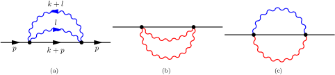
Figure 3: Two loop contribution of diamagnetic gauge interactions to wave function renormalization of $Y,Y^{\dagger}$. They contribute to $\mathbb{I}$ operator in the dilatation operator.

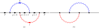
Figure 4: Two loop contribution of paramagnetic gauge interactions to wave function renormalization of $Y,Y^{\dagger}$. They contribute to $\mathbb{I}$ operator in the dilatation operator.

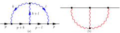
Figure 5: Two loop contribution of Chern-Simons interaction to wave function renormalization of $Y,Y^{\dagger}$. They contribute to $\mathbb{I}$ operators in the dilatation operator.

For the gauge diamagnetic contribution depicted in Fig. 3, only the last one is of mixed type. For the $M=N$ case, each diagram contributes respectively by $-{\lambda^{2}\over 24}{\mathbb{I}}$, $-{\lambda^{2}\over 24}{\mathbb{I}}$ and ${\lambda^{2}\over 6}{\mathbb{I}}$ to the anomalous dimension for each site, which add up to ${\lambda^{2}\over 12}{\mathbb{I}}$. For the present case, their contribution is then

$$H^{\rm dia}_{\rm\ Z} = \Big{[}\ -{\lambda^{2}\over 24}-{{\bar{\lambda}}^{2}\over 24}+{\lambda\bar{\lambda}\over 6}\Big{]}\sum_{\ell=1}^{2L}\mathbb{I}\,.$$ (4.10)

The contributions of the gauge paramagnetic interaction in Fig. 4 are obviously all mixed type. Hence, their contribution becomes

$$H^{\rm para}_{\rm\ Z} = {2\lambda\bar{\lambda}\over 3}\sum_{\ell=1}^{2L}\mathbb{I}\,.$$ (4.11)

The contributions of the Chern-Simons interaction in Fig. 5 are of types $\lambda^{2}$ or ${\bar{\lambda}}^{2}$. Its contribution now becomes

$$H^{\rm cs}_{\rm\,\,Z} = \Big{[}\ {\lambda^{2}\over 6}+{{\bar{\lambda}}^{2}\over 6}\Big{]}\sum_{\ell=1}^{2L}\mathbb{I}\,.$$ (4.12)

The fermion pair interactions to the wave function renormalization are depicted in Fig. 6 and they are all of mixed type. Their contributions are

$$H^{\rm yukawa}_{\rm\ Z} = \lambda\bar{\lambda}\Big{[}\ {4\over 3}+1\Big{]}\sum_{\ell=1}^{2L}\mathbb{I}\,.$$ (4.13)

Finally, we consider the two-loop contribution from the vacuum polarization. Since the Chern-Simons gauge loop and the corresponding ghost loop contributions cancel with each other precisely, only the matter loops have the non-vanishing contributions. The non-vanishing two loop contributions of vacuum polarizations are all mixed type, which are depicted in Fig. 7. Their contribution is

$$H^{\rm vacuum}_{\rm\ Z} = -{8\lambda\bar{\lambda}\over 3}\sum_{\ell=1}^{2L}\mathbb{I}\,.$$ (4.14)

Summing up all these wave function renormalization to $Y,Y^{\dagger}$, we find their contribution to the anomalous dimension matrix as

$$H_{\rm\,\,Z} = \Big{[}\ {\lambda^{2}\over 8}+{{\bar{\lambda}}^{2}\over 8}+{\lambda\bar{\lambda}\over 2}\Big{]}\sum_{\ell=1}^{2L}\mathbb{I}\,.$$ (4.15)

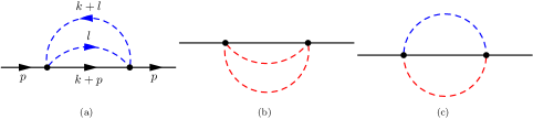
Figure 6: Two loop contribution of fermion pair interaction to wave function renormalization of $Y,Y^{\dagger}$. They contribute to $\mathbb{I}$ operators in the dilatation operator.

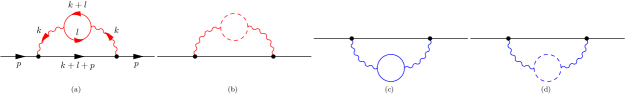
Figure 7: Two loop contribution of vacuum polarization to wave function renormalization of $Y,Y^{\dagger}$.

One can see that the $\lambda^{2}$ and ${\bar{\lambda}}^{2}$ contributions in (4.15) cancel with those of (4.7). Thus, one finds that only mixed type contributions remain. Adding up all contributions,

$$H_{\rm total} = H_{\rm B}+H^{\rm gauge}_{\rm\,\,I}+H_{\rm F}+H^{\rm gauge}_{\rm\,\,K}+H_{\rm Z}$$ (4.16)

we get the result (4.5). As claimed, this is precisely the parity-symmetric alternating spin chain Hamiltonian we obtained from the mixed set of the relevant Yang-Baxter equations.

Finally, let us comment on the two loop wrapping interaction of $L=1$ case as a checkpoint of internal consistency with ${\cal N}=6$ supersymmetry, extended to $M\neq N$. The ${\bf 4}\otimes{\bf\bar{4}}$ representation is decomposed irreducibly into the traceless part, $\bf 15$, and the trace part, $\bf{1}$. The multiplet $\bf 15$ is chiral primary operator, so their conformal dimension ought to be protected by supersymmetry. However there is no contribution of three-site scalar interaction. Thus naively, the protection of the above chiral primary operator is not possible. However, spectrum of the gauge invariant operator of length $2L=2$ will receive contributions from wrapping diagrams already at leading order, which we will identify.

From the above computations, the sum of the two-site and the one-site contributions is

$$H_{2}+H_{1}=\lambda{\bar{\lambda}}\Big{[}\ {1\over 2}\mathbb{K}+{1\over 2}\mathbb{I}\ \Big{]}\times 2=\lambda{\bar{\lambda}}\Big{[}\mathbb{K}+\mathbb{I}\Big{]}\,,$$ (4.17)

where the multiplication factor two comes from the number of sites.

The wrapping contributions in Fig.8 are all mixed type. The evaluation of the corresponding Feynman integrals are the same as the case of $M=N$ except replacing $\lambda^{2}$ by $\lambda\bar{\lambda}$.

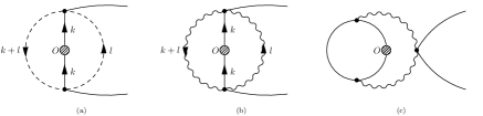
Figure 8: Two loop wrapping interaction contribution to the shortest gauge invariant operators. (a) fermion field wrapping, (b) gauge field wrapping, (c) a new gauge triangle.

The results is

$$H_{\rm wrap}=\lambda{\bar{\lambda}}\Big{[}\ \mathbb{I}+2(\mathbb{K}-\mathbb{I})-\mathbb{K}\ \Big{]}=\lambda{\bar{\lambda}}\Big{[}\mathbb{K}-\mathbb{I}\Big{]}\,,$$ (4.18)

Putting both the original and the wrapping diagram contributions together, the full Hamiltonian of $2L=2$ operator is given by

$$H_{2L=2}=2\,\lambda\bar{\lambda}\,\mathbb{K}\,.$$ (4.19)

Notice that the part proportional to $\mathbb{I}$ operator is canceled between the original and the wrapping interaction contributions. One thus check that the chiral primary operators $\bf 15$ indeed has a vanishing anomalous dimension since, by definition, it has no trace part and is annihilated by $\mathbb{K}$ operator. For the singlet ${\bf 1}$, $|s\rangle={1\over 2}|II\rangle$, the anomalous dimension is

$$H|s\rangle=8\,\,\lambda\bar{\lambda}\,\,|s\rangle\,.$$ (4.20)

So far, we computed the spectrum of the shortest operators without a priori assumption of supersymmetry. As a consistency check, we now compare these spectra with their superpartners. Recall that length $2\ell$ operators with Dynkin labels $(\ell-2m,m+n,\ell-2n)$ and length $2\ell-2$ operators with Dynkin labels $(\ell-2m,m+n-2,\ell-2n)$ are superpartners each other. Here, we have the simplest situation: the $L=1$ operator ${\bf 1}$ of Dynkin labels $(0,0,0)$ is the superpartner of $L=2$ operator ${\bf 20}$ of Dynkin labels $(0,2,0)$. Using the results of Ref. [5], the anomalous dimension of the latter can be found as $8\lambda\bar{\lambda}$, and matches perfectly with our computation.

5 Further Discussions

The most salient feature of our results is that, though the Yang-Baxter equations and hence the integrability structure permit it, the spin chain Hamiltonian derived from the ABJ theory at two loops does not show parity symmetry breaking. In this section, we elaborate further regarding this result and also provide intuitive (albeit heuristic) argument for the reason why.

• Weak Coupling Limit: Closed Spin Chains The spin chain is, roughly speaking, weak coupling counterpart of the semiclassical string propagating on AdS${}_{4}\times\mathbb{CP}_{3}$ with discrete $B_{\rm NS}$ holonomy. On the other hand, the supergravity dual background of the ABJ theory is given by

  $${\rm d}s^{2} = R^{2}_{s}\left[{1\over 4}{\rm d}s^{2}(\mbox{AdS}_{4})+{\rm d}s^{2}(\mathbb{CP}_{3})\right]$$

  $$e^{2\phi} = {R_{s}^{2}\over k^{2}}$$

  $$F_{4} = {3\over 8}kR_{s}^{2}\widehat{\epsilon}_{4}$$

  $$F_{2} = k{\rm d}\omega=k\,J$$

  $$B_{\rm NS} = b\,J\,,$$ (5.1)

  where $J$ is the Kähler two-form threading the $\mathbb{CP}^{1}$ inside $\mathbb{CP}^{3}$. Notice that the curvature radius is

  $$R^{2}_{s}=2^{5\over 2}\pi\sqrt{\lambda}\,,$$ (5.2)

  is exactly the same as the background of ABJM theory, viz. the curvature radius remains unchanged by turning on the $B_{\rm NS}$ holonomy. As such, the spectrum of light fields is unaffected by the discrete $B_{\rm NS}$ holonomy. This is consistent with ABJ’s claim that the spectrum of all non-baryonic chiral primary operators is independent of $b$ but also goes beyond, asserting that all string spectrum is independent of the discrete holonomy.

  Given that the spectrum of chiral primary operators is independent of $b$, it is not surprising that the spectrum of all single trace operators (2.5) is also independent of $b$ as well. Consider a closed, semiclassical string propagating in the background (5.1). The string is macroscopic and propagates freely with the worldsheet topology of cylinder. This is the strong coupling counterpart of a single trace operator in the planar limit. Since the worldsheet has topology of cylinder, the integral over the pullback of the discrete $B_{\rm NS}$ holonomy would be zero. ABJ argues further that, at strong ‘t Hooft coupling regime, all the U$(M)_{k}\times\overline{\rm U(N)}_{-k}$ theories with $M=N,N+1,\cdots,N+k$ are all similar to each other, since the only difference is the discrete $B_{\rm NS}$ holonomy. Extrapolating this to the weak ‘t Hooft coupling regime, it then seems that all these theories are identical to all orders in the planar perturbation theory. Our result that the spin chain Hamiltonian of single trace operators is parity invariant fits to these ABJ arguments.

  On the other hand, if the string trajectory wraps around $\mathbb{CP}_{1}$ over which the discrete $B_{\rm NS}$ holonomy is turned on, the integral will be nonzero. In fact, this leads to the worldsheet instanton effect whose strength scales as $\exp(-\sqrt{\lambda})$. Transcribed to the weak coupling limit, we conjecture that these worldsheet instanton effects may correspond to a class of unsuppressed fluctuations of the length of the single trace operators. These fluctuations are not generic ones, since they must be the counterpart of worldsheet topology of sphere. At present, though, it is unclear what precise nature of these fluctuations are.

  Putting these considerations together, the $(M-N)$ dependent effect is completely suppressed at the strong ‘t Hooft coupling limit (modulo worldsheet instanton effect) and is most pronounced at the weak ‘t Hooft coupling limit, as reflected through the coupling parameter $\lambda\overline{\lambda}=\lambda^{2}(1+b/\lambda)$. Still, we found that the parity symmetry breaking effect, proportional to the sign of $(M-N)$, is invisible in the single trace operators.

• Strong Coupling Limit: Giant Magnon Is the parity symmetry breaking visible at strong coupling limit, $\lambda,\overline{\lambda}\rightarrow\infty$? Because of quantum consistency, as discussed in Section 2, the coupling parameter $b$ is restricted to a discrete value ranging over $[0,1]$. Therefore, in the limit $\lambda,\overline{\lambda}\rightarrow\infty$, we expect that parity symmetry breaking effect is completely suppressed to the order ${\cal O}(1/\lambda,1/\overline{\lambda})$. Below, we confirm such expectation by demonstrating that the spectrum of a giant magnon in the gravity dual of the ABJ theory is exactly the same as that in the gravity dual of the ABJM theory.

  We parametrize the $\mathbb{CP}_{3}$ metric as

  $${\rm d}s^{2} = {\rm d}\xi^{2}+{\sin^{2}2\xi\over 4}\left({\rm d}\psi+{\cos\theta_{1}\over 2}{\rm d}\phi_{1}-{\cos\theta_{2}\over 2}{\rm d}\phi_{2}\right)^{2}+{1\over 4}\cos^{2}\xi({\rm d}\theta_{1}^{2}+\sin^{2}\theta_{1}{\rm d}\phi_{1}^{2})$$ (5.3)

  $$+ {1\over 4}\sin^{2}\xi({\rm d}\theta_{2}^{2}+\sin^{2}\theta_{2}{\rm d}\phi_{2}^{2})\,.$$

  The $B_{\rm NS}$ potential is

  $$B_{\rm NS}=-{b\over 2}\Bigl{(}{\sin 2\xi}{\rm d}\xi\wedge\left(2{\rm d}\psi+{\cos\theta_{1}}{\rm d}\phi_{1}-{\cos\theta_{2}}{\rm d}\phi_{2}\right)\Bigr{.}$$

  $$\ \ \ \ \Bigr{.}+\cos^{2}\xi\sin\theta_{1}{\rm d}\theta_{1}\wedge{\rm d}\phi_{1}+\sin^{2}\xi\sin\theta_{2}{\rm d}\theta_{2}\wedge{\rm d}\phi_{2}\Bigl{)}\,.$$ (5.4)

  We work in the conformal gauge-fixing and choose the static gauge $t=\tau$. We truncate the dynamics consistently on the first $\mathbb{S}^{2}$ by setting $\xi=0$ and rename $\theta_{1}=\theta,\phi_{1}=\phi$. Bosonic part of the Type IIA superstring worldsheet action over $\mathbb{R}_{t}\times\mathbb{S}^{2}$ reads

  $$S=\int{\rm d}\tau\int^{r}_{-r}{\rm d}\sigma\Big{[}{\pi\sqrt{2\lambda}\over 4\pi}\Big{(}{(\partial z)^{2}\over 1-z^{2}}+(1-z^{2})(\partial\phi)^{2}\Big{)}+{b\over 4\pi}(\dot{z}\phi^{\prime}-{z^{\prime}}\dot{\phi})\Big{]}$$ (5.5)

  where $z=\cos\theta$. In this set-up, the Virasoro constraints

  $${{\dot{z}}^{2}+{z^{\prime}}^{2}\over 1-z^{2}}+(1-z^{2})({\dot{\phi}}^{2}+{\phi^{\prime}}^{2})=1\,,$$

  $${\dot{z}\,\,z^{\prime}\over 1-z^{2}}+(1-z^{2})\dot{\phi}\,\,{\phi^{\prime}}=0$$ (5.6)

  have to be imposed as well. The energy density is uniform in the static gauge and the string energy is proportional to the spatial coordinate size:

  $$E={\pi\sqrt{2\lambda}\over 2\pi}\,\,2r\,.$$ (5.7)

  With an ansatz,

  $$z=z(\sigma-v\omega t)\,,\,\ \ \ \ \phi=\omega\tau+\varphi(\sigma-v\omega t)\,,$$ (5.8)

  the equations of motion are reduced to

  $$(z^{\prime})^{2}={\omega^{2}\over(1-v^{2}\omega^{2})^{2}}\left(z^{2}-1+{1\over\omega^{2}}\right)\left(1-v^{2}-z^{2}\right)$$

  $$\varphi^{\prime}={v\omega^{2}\over(1-v^{2}\omega^{2})}{z^{2}-1+{1\over\omega^{2}}\over 1-z^{2}}\,.$$ (5.9)

  The equation of motion is not affected by the $B_{\rm NS}$ field. The worldsheet momentum $p$ is from the $\int^{r}_{-r}(x_{-})^{\prime}$ with $x_{-}=t+\phi$, which equals to $\Delta\phi$. Hence it is independent of $b$. The expression for the angular momentum is affected by

  $$J=\int^{r}_{-r}\left({\pi\sqrt{2\lambda}\over 4\pi}(1-z^{2})\dot{\phi}-{b\over 4\pi}z^{\prime}\right)$$ (5.10)

  but, on the solution, its value does not change due to the boundary condition of $z(-r)=z(r)$. The general solution can found as [24]

  $$z={\sqrt{1-v^{2}}\over\omega\sqrt{\eta}}{\rm dn}\left({\sigma-v\tau\over\sqrt{\eta}\sqrt{1-v^{2}}}\,,\eta\right)$$ (5.11)

  where ${\rm dn}(\sigma,k^{2})$ is the Jacobi elliptic function and we introduced the parameter $\eta$ by

  $$\eta={1-\omega^{2}v^{2}\over\omega^{2}(1-v^{2})}\,.$$ (5.12)

  The range parameter $r$ is given by $\sqrt{1-v^{2}}\sqrt{\eta}K(\sqrt{\eta})$ where $K(x)$ is the complete elliptic integral. For simplicity, consider the infinite size limit $\omega\rightarrow 1$ . The solution in this limit becomes

  $$z=\sqrt{1-v^{2}}{\rm sech}\left({\sigma-v\tau\over\sqrt{1-v^{2}}}\right)\,.$$ (5.13)

  with the worldsheet momentum given by $p=2\cos^{-1}v$. The spectrum

  $$E-J=\sqrt{2\lambda}\left|\sin{p\over 2}\right|\,,$$ (5.14)

  remains unchanged, thus showing no $b$-dependence nor parity symmetry breaking effect.

• Weak Coupling Limit Revisited: Open Spin Chain Though effect of the discrete $B_{\rm NS}$ holonomy is invisible to closed strings (up to the aforementioned worldsheet instanton effect), the holonomy certainly affects spectrum of heavier string states such as D-branes that wrap around $\mathbb{CP}_{1}$ over which the discrete $B_{\rm NS}$ holonomy is turned on. These D-branes are giant gravitons and di-baryons and their excitation is described by open strings attached to them. Again, as for the closed string case, we see that the effect is suppressed in large ‘t Hooft coupling limit, while it could be pronounced in small ‘t Hooft coupling limit. From the string worldsheet action (5.5), we expect that the boundary condition gives rise to at most ${\cal O}(1/\lambda)$ effect.

  Transcribed again to the weak ‘t Hooft coupling regime, a natural setting where the parity symmetry breaking can be seen is the open spin chain attached to giant gravitons or baryonic operators. The effect of $(M-N)$ should be reflected to possible types boundary condition of the open spin chain. For example, since the $B_{\rm NS}$ holonomy takes $(M-N)$ discrete values, we expect that there are $(M-N)$ types of boundary conditions. For gauge group U$(M)\times\overline{{\rm U}(N)}$, the baryonic operator $\epsilon_{a_{1}\cdots a_{M}}\epsilon^{b_{1}\cdots b_{N}}{Y^{I_{1}a_{1}}}_{b_{1}}\cdots{Y^{I_{N}a_{N}}}_{b_{N}}$ is not a gauge singlet but transforms as $(M-N)$-th antisymmetric product of fundamentals of the U$(M)$ gauge group. It is natural to expect that the $(M-N)$ types of open spin chain boundary conditions are associated with the multiplicity of these baryonic operator. For ${\cal N}=4$ super Yang-Mills theory, such configuration of open spin chain was studied [25]. In fact, boundary reflection matrices were determined for the tensor structure [26] and for the dressing phases [27, 28]. We expect similar development can be made in the ABJ theory with the new twist of the multiple boundary conditions. We are currently investigating this and will report the results elsewhere.

Finally, since the spin chain Hamiltonian of the ABJ theory takes the same form as the ABJM theory, diagonalization of the transfer matrices proceeds the same manner. Thus, the Bethe ansatz equations of SO(6) sector [5, 6] and of full OSp$(6|4,\mathbb{R})$ [5] will have exactly the same form except that $\lambda^{2}$ of the ABJM theory counterpart is now replaced by $\lambda\overline{\lambda}$.

Appendix A ${\cal N}=6$ ${\rm U(M)}\times\overline{\rm U(N)}$ Super Chern-Simons Theory

$\bullet$ Gauge and global symmetries:

$$\mbox{gauge symmetry}:\quad\mbox{U(M)}\otimes\overline{\mbox{U(N)}}$$

$$\mbox{global symmetry}:\quad\mbox{SU(4)}$$ (A.1)

We denote trace over U(M) and $\overline{\rm U(N)}$ as Tr and $\overline{\rm Tr}$, respectively.

$\bullet$ On-shell fields are gauge fields, complexified Hermitian scalars and Majorana spinors ($I=1,2,3,4$):

$$A_{m}:\quad\mbox{Adj}\,\,\,(\mbox{U(M)});\hskip 56.9055pt\overline{A}_{m}:\quad\mbox{Adj}\,\,\,\overline{\mbox{U(N)}}$$

$$Y^{I}=(X^{1}+iX^{5},X^{2}+iX^{6},X^{3}-iX^{7},X^{4}-iX^{8}):\qquad({\bf M},\overline{\bf N};{\bf 4})$$

$$Y^{\dagger}_{I}=(X^{1}-iX^{5},X^{2}-iX^{6},X^{3}+iX^{7},X^{4}+iX^{8}):\hskip 22.76228pt(\overline{\bf M},{\bf N};\overline{\bf 4})$$

$$\Psi_{I}=(\psi^{2}+i\chi^{2},-\psi^{1}-i\chi^{1},\psi_{4}-i\chi_{4},-\psi_{3}+i\chi_{3}):\hskip 11.38092pt({\bf M},\overline{\bf N};\overline{\bf 4})$$

$$\Psi^{\dagger I}=(\psi_{2}-i\chi_{2},-\psi_{1}+i\chi^{1},\psi^{4}+i\chi^{4},-\psi^{3}-i\chi^{3}):\hskip 8.5359pt(\overline{\bf M},{\bf N};{\bf 4})$$ (A.2)

$\bullet$ action:

$$I = \int_{\mathbb{R}^{1,2}}\Big{[}\,{k\over 4\pi}\epsilon^{mnp}\mbox{Tr}\left(A_{m}\partial_{n}A_{p}+{2i\over 3}A_{m}A_{n}A_{p}\right)-{k\over 4\pi}\epsilon^{mnp}\overline{\mbox{Tr}}\left(\overline{A}_{m}\partial_{n}\overline{A}_{p}+{2i\over 3}\overline{A}_{m}\overline{A}_{n}\overline{A}_{p}\right)$$ (A.3)

$$\hskip 28.45274pt+{1\over 2}\overline{\mbox{Tr}}\left(-(D_{m}Y)^{\dagger}_{I}D^{m}Y^{I}+i\Psi^{\dagger I}D\hskip-6.25963pt/\Psi_{I}\right)+{1\over 2}\mbox{Tr}\left(-D_{m}Y^{I}(D^{m}Y)^{\dagger}_{I}+i\Psi_{I}D\hskip-6.25963pt/\Psi^{\dagger I}\right)$$

$$\hskip 28.45274pt-V_{\rm F}-V_{\rm B}\,\Big{]}$$

Here, covariant derivatives are defined as

$$D_{m}Y^{I}=\partial_{m}Y^{I}+iA_{m}Y^{I}-iY^{I}\overline{A}_{m}\,,\quad D_{m}Y^{\dagger}_{I}=\partial_{m}Y^{\dagger}_{I}+i\overline{A}_{m}Y^{\dagger}_{I}-iY^{\dagger}_{I}A_{m}$$ (A.4)

and similarly for fermions $\Psi_{I},\Psi^{\dagger I}$. Potential terms are

$$V_{\rm F} = {2\pi i\over k}\overline{\mbox{Tr}}\Big{[}Y^{\dagger}_{I}Y^{I}\Psi^{\dagger J}\Psi_{J}-2Y^{\dagger}_{I}Y^{J}\Psi^{\dagger I}\Psi_{J}+\epsilon^{IJKL}Y^{\dagger}_{I}\Psi_{J}Y^{\dagger}_{K}\Psi_{L}]$$ (A.5)

$$- {2\pi i\over k}\mbox{Tr}[Y^{I}Y^{\dagger}_{I}\Psi_{J}\Psi^{\dagger J}-2Y^{I}Y^{\dagger}_{J}\Psi_{I}\Psi^{\dagger J}+\epsilon_{IJKL}Y^{I}\Psi^{\dagger J}Y^{K}\Psi^{\dagger L}\Big{]}$$

and

$$V_{\rm B} = -{1\over 3}\left({2\pi\over k}\right)^{2}\overline{\mbox{Tr}}\Big{[}\,Y^{\dagger}_{I}Y^{J}Y^{\dagger}_{J}Y^{K}Y^{\dagger}_{K}Y^{I}+Y^{\dagger}_{I}Y^{I}Y^{\dagger}_{J}Y^{J}Y^{\dagger}_{K}Y^{K}$$ (A.6)

$$\hskip 51.21504pt+4Y^{\dagger}_{I}Y^{J}Y^{\dagger}_{K}Y^{I}Y^{\dagger}_{J}Y^{K}-6Y^{\dagger}_{I}Y^{I}Y^{\dagger}_{J}Y^{K}Y^{\dagger}_{K}Y^{J}\,\Big{]}$$

At quantum level, since the Chern-Simons term shifts by an integer multiple of $8\pi^{2}$, $k$ should be integrally quantized.

References

- [1] O. Aharony, O. Bergman, D. L. Jafferis and J. Maldacena, “N=6 superconformal Chern-Simons-matter theories, M2-branes and their gravity duals,” arXiv:0806.1218 [hep-th].
- [2] O. Aharony, O. Bergman and D. L. Jafferis, “Fractional M2-branes,” arXiv:0807.4924 [hep-th].
- [3] B. E. W. Nilsson and C. N. Pope, Class. Quant. Grav. 1 (1984) 499.
- [4] K. Hosomichi, K. M. Lee, S. Lee, S. Lee and J. Park, “N=5,6 Superconformal Chern-Simons Theories and M2-branes on Orbifolds,” arXiv:0806.4977 [hep-th].
- [5] J. A. Minahan and K. Zarembo, “The Bethe ansatz for superconformal Chern-Simons,” arXiv:0806.3951 [hep-th].
- [6] D. Bak and S. J. Rey, “Integrable Spin Chain in Superconformal Chern-Simons Theory,” JHEP 0810 (2008) 053 [arXiv:0807.2063 [hep-th]].
- [7] T. Nishioka and T. Takayanagi, “On Type IIA Penrose Limit and N=6 Chern-Simons Theories,” arXiv:0806.3391 [hep-th].
- [8] D. Gaiotto, S. Giombi and X. Yin, “Spin Chains in N=6 Superconformal Chern-Simons-Matter Theory,” arXiv:0806.4589 [hep-th].
- [9] E. G. Gimon and J. Polchinski, Phys. Rev. D 54 (1996) 1667 [arXiv:hep-th/9601038].
- [10] M. R. Douglas, JHEP 9707 (1997) 004 [arXiv:hep-th/9612126].
- [11] S. S. Gubser and I. R. Klebanov, Phys. Rev. D 58 (1998) 125025 [arXiv:hep-th/9808075].
- [12] K. Dasgupta and S. Mukhi, JHEP 9907 (1999) 008 [arXiv:hep-th/9904131].
- [13] I. R. Klebanov and A. A. Tseytlin, Nucl. Phys. B 578 (2000) 123 [arXiv:hep-th/0002159].
- [14] I. R. Klebanov and M. J. Strassler, JHEP 0008 (2000) 052 [arXiv:hep-th/0007191].
- [15] See, for example, N. Beisert, B. Eden and M. Staudacher, J. Stat. Mech. 0701 (2007) P021 [arXiv:hep-th/0610251]; L. Freyhult, A. Rej and M. Staudacher, J. Stat. Mech. 0807 (2008) P07015 [arXiv:0712.2743 [hep-th]] and references to earlier works therein.
- [16] A. Hanany and E. Witten, Nucl. Phys. B 492 (1997) 152 [arXiv:hep-th/9611230].
- [17] S. J. Rey, unpublished note (1997).
- [18] G. Arutyunov and S. Frolov, “Superstrings on as a Coset Sigma-model,” arXiv:0806.4940 [hep-th].
- [19] B. J. Stefanski, “Green-Schwarz action for Type IIA strings on ,” arXiv:0806.4948 [hep-th].
- [20] N. Gromov and P. Vieira, “The AdS4/CFT3 algebraic curve,” arXiv:0807.0437 [hep-th].
- [21] D. Gaiotto and X. Yin, JHEP 0708 (2007) 056 [arXiv:0704.3740 [hep-th]].
- [22] H. J. de Vega and F. Woynarovich, J. Phys. A 25, 4499 (1992).
- [23] E. Ragoucy and G. Satta, JHEP 0709, 001 (2007) [arXiv:0706.3327 [hep-th]].
- [24] G. Arutyunov, S. Frolov and M. Zamaklar, Nucl. Phys. B 778 (2007) 1 [arXiv:hep-th/0606126].
-
[25]
O. DeWolfe and N. Mann,
JHEP 0404 (2004) 035
[arXiv:hep-th/0401041];
D. Berenstein and S. E. Vazquez, JHEP 0506, 059 (2005) [arXiv:hep-th/0501078];
T. Erler and N. Mann, JHEP 0601, 131 (2006) [arXiv:hep-th/0508064];
K. Okamura and K. Yoshida, JHEP 0609, 081 (2006) [arXiv:hep-th/0604100];
D. Berenstein, D. H. Correa and S. E. Vazquez, JHEP 0609, 065 (2006) [arXiv:hep-th/0604123];
N. Mann and S. E. Vazquez, JHEP 0704, 065 (2007) [arXiv:hep-th/0612038]. - [26] D. M. Hofman and J. M. Maldacena, JHEP 0711, 063 (2007) [arXiv:0708.2272 [hep-th]].
- [27] H. Y. Chen and D. H. Correa, JHEP 0802 (2008) 028 [arXiv:0712.1361 [hep-th]].
- [28] C. Ahn, D. Bak and S. J. Rey, JHEP 0804 (2008) 050 [arXiv:0712.4144 [hep-th]].