Statistical physics of cerebral embolization leading to stroke

Abstract

We discuss the physics of embolic stroke using a minimal model of emboli moving through the cerebral arteries. Our model of the blood flow network consists of a bifurcating tree, into which we introduce particles (emboli) that halt flow on reaching a node of similar size. Flow is weighted away from blocked arteries, inducing an effective interaction between emboli. We justify the form of the flow weighting using a steady flow (Poiseuille) analysis and a more complicated nonlinear analysis. We discuss free flowing and heavily congested limits and examine the transition from free flow to congestion using numerics. The correlation time is found to increase significantly at a critical value, and a finite size scaling is carried out. An order parameter for non-equilibrium critical behavior is identified as the overlap of blockages’ flow shadows. Our work shows embolic stroke to be a feature of the cerebral blood flow network on the verge of a phase transition.

I Introduction

Stroke is a common cause of death and disability, and is expected to become more prevalent as average life expectancy increases Lopez and Murray (1998). A common cause of stroke is from embolisation, where small pieces of thrombus and plaque detach from the insides of diseased arteries and move through the vasculature to become lodged in arteries supplying the brain. Depending on the duration and position of the obstruction, embolic blockages can prove fatal.

Doppler ultrasound embolus detection in individuals at high risk of stroke reveals that large numbers of emboli typically enter the cerebral circulation in advance of a major stroke occurring Mackinnon et al. (2005). Embolus detection and autopsy studies of patients who have undergone cardiovascular surgery show that patients can experience several thousand emboli during typical heart surgery Moody et al. (1990) (which carries a 3-10% stroke risk Bucerius et al. (2003)). The interplay between these emboli is governed by flow dynamics, and thus the onset of stroke can be considered as a complex process of arterial obstruction involving multiple blockages. However, little is currently understood about the impact of multiple emboli leading to the onset of stroke.

To gain a better understanding of the triggers leading to the onset of stroke from multiple emboli, we developed a probabilistic Monte Carlo approach to predict the severity of arterial obstruction Chung et al. (2007). Our model is non-trivial because blockages divert the flow of new emboli that enter the arteries (i.e. there is an effective interaction between emboli). We predicted a very rapid change from free-flow with little occlusion to severely obstructed arteries as the size of the emboli increased, which we suspected was associated with a phase transition. In this article, we examine the origins of this behavior more closely.

This article is organized as follows. In section II, we introduce our model and algorithm, and carry out a basic fluid dynamical analysis of the vascular tree to justify our flow weighting scheme. To gain more insight into the model, we determine the limiting properties of the model in section III. To better understand the motion of emboli through the tree, we examine space-time plots of blockages in a single realization of the model (section V). We examine the time correlator and correlation time in Sec. IV. The order parameter is examined in Sec. V. Finally, we summarize our results in section VI.

II Model

II.1 Vasculature

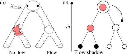
Figure 1: A representation of a small section of the cerebral vasculature. (a) Arteries supplying the brain typically bifurcate. The number of branches in the vasculature is prohibitively large for a full fluid-dynamical analysis. For this reason, we develop a minimal model (b) where nodes on a bifurcating tree represent arteries which can become blocked. When emboli block nodes, blood flow is weighted according to the number of nodes at the bottom of the tree receiving unimpeded flow. The flow carries new emboli away from existing blockages, introducing an effective interaction between emboli.

We treat the cerebral vasculature as a bifurcating tree, which is consistent with high resolution images showing that $>97\%$ of all branches in the cerebral arteries are bifurcations Cassot et al. (2006). In this study, we do not consider the largest vessels such as the circle of Willis (CoW). Since most emboli travel into the middle carotid artery (MCA) after passing through the CoW, we consider our model to be a simplified version of the cerebral arteries supplied by the MCA. Bifurcations can be characterized by the bifurcation exponent, which is defined through the relation $x_{s}^{\gamma}=2x_{d}^{\gamma}$ where $x_{s}$ and $x_{d}$ are the respective radii of the source and daughter vessels Karshafian et al. (2003). In this study, we use a single bifurcation exponent of $\gamma$ at all levels of the tree. When the bifurcation exponent is greater than $2$, the total cross sectional area of the daughter vessels is greater than that of the source vessel. In many organisms, the bifurcation exponent is expected to be approximately $3$ Murray (1926). A schematic of our model vasculature is shown in Fig. 1. We vary $M_{\ell}$ (the total number of layers in our tree) so that the vessel sizes range from $x_{\rm max}=1$mm to a few $\mu$m ($x_{\rm min}$), which is similar to the dimensions of the arteries in the brain. Node diameters are $x_{m}=x_{\rm min}2^{m/\gamma}$ with $m$ the level of the tree ($m=0$ corresponds to the smallest arteries and $m=M_{\ell}-1$ to the largest). The nodes are connected by segments representing arteries.

II.2 Fluid dynamics and flow weighting

Figure 2: (a) Flow weighting on small symmetric trees where the drop in pressure obeys Poiseuille’s equation, and the bifurcation exponent $\gamma=3$. Flow resistances were assumed to change with tree level according to Eqn. 4. (b) Flow weighting on small symmetric trees where pressure differences have a nonlinear dependence on the flow according to Eqn. 5 and $\gamma=3$. The flow weightings tend towards the linear weighting scheme with increasing system size.

Emboli are carried by the blood, and as will be discussed in sec. II.3, the trajectory of emboli at a bifurcation is related to the relative flow in the branches. Since obstruction by emboli causes redirection of blood-flow, it is relevant to determine the ratio of flows in the network downstream from a bifurcation in the presence of blockages using a basic fluid dynamical analysis.

For initial determination of how the flow is modified by blockages downstream of a bifurcation, it is convenient to assume that flow in segments of the tree obeys Poiseuille’s law,

$$\Delta P=\left(\frac{8\mu l}{\pi a^{4}}\right)q\equiv Rq$$ (1)

where $\mu$ is the blood viscosity, $a$ is the radius of the artery, $l$ is the length of the segment of the artery that is being considered, $q$ is the volume flow through the vessel, $R$ is the resistance of the vessel to flow, and $\Delta P$ is the pressure drop over a vessel segment. By following all possible routes from the root node where the pressure is $P_{A}$ to the capillary mesh where pressure is $P_{V}$, a set of $2^{N-1}$ equations can be determined,

$$\sum_{n=0}^{N-1}R_{n,i(n)}q_{n,i(n)}=P_{A}-P_{V}$$ (2)

which are supplemented by $2^{N-1}-1$ simultaneous equations of the form

$$q_{n,i}-q_{n-1,2i-1}-q_{n-1,2i}=0$$ (3)

derived from conservation of flow to give $2^{N}-1$ equations for the $2^{N}-1$ flows in the tree. The nomenclature $q_{n,i}$ indicates the $i$th node in the $n$th level.

It remains to assign realistic values to the resistances. The lengths of arteries are proportional to their radii $l=\kappa a$ West et al. (1997) and the radii typically follow Murray’s law $a_{n-1}^{\gamma}=2a_{n}^{\gamma}$ with the bifurcation exponent normally $\gamma=3$ Murray (1926) (note that in this section only, $n=0$ is the root node, with $n$ increasing on entering the tree). Thus $R_{n}\propto a^{-3}\propto 2^{3n/\gamma}$. Replacing the coefficients,

$$R_{n}=\frac{8\mu\kappa 2^{3n/\gamma}}{\pi a_{0}^{3}}$$ (4)

$a_{0}$ is the radius of the root node. Following standard theoretical practice, the ratio of segment length to segment radius is set as $l=20a$, i.e. $\kappa=20$ Zamir (1999).

It is straightforward to invert the simultaneous equations to establish the proportion of total flow into a daughter vessel, $f=q_{A}/(q_{A}+q_{B})$, the proportion of flow in direction $A$ at a bifurcation as $X$ (the ratio of free nodes in direction $A$ to total free nodes) is changed (the flow in daughter vessels $A$ and $B$ is $q_{A}$ and $q_{B}$ respectively) . The result is shown in figure 2(a). As the tree size grows, the relative resistance of the end vessels increases as compared to the root node, and the flow solution approaches the line $f=X$. For $\gamma<3$ the linear approximation is even more closely approached.

Directly downstream from a bifurcation, Poiseuille flow is not fully formed, leading to an increased pressure drop which depends nonlinearly on the flow according to the formula Cieslicki and Ciesla (2005),

$$\Delta P=R\left(q+\frac{0.176q^{2}\rho}{l\pi\mu}\right),$$ (5)

here $\rho$ the density of the fluid. We solve the set of equations resulting from replacing Poiseuille’s law for the nonlinear pressure drop of equation 5 (using the results from the linear flow analysis as an initial solution) showing the results in Fig. 2(b). Again, the line $f=X$ is approached as the size of the tree in increased. The approach is less rapid than that found with the Poiseuille analysis, but for very large trees, a linear relation between the ratio of free arterioles to the ratio of flows is expected.

The results of the basic fluid dynamical analysis indicate that a linear flow weighting scheme is a good approximation to the true fluid dynamics. The linear weighting approximation is strictly valid in the limit that the flow resistance in the capillary nodes is much higher than in any of the other nodes. It is also known from studies of vascular physiology that most pressure is dropped across the smallest arterioles (see e.g. Ref. Levick (2003)) giving further evidence for the validity of a linear weighting approximation.

II.3 Embolus trajectory at bifurcation

Figure 3: $r$ vs $f$ at a bifurcation. Data shown as solid points are taken from in vitro measurements by Bushi et al. Bushi et al. (2005). Our parameterization of the experimental data via equation 6 is shown as the dotted line.

The response of an embolus to flow at a bifurcation is complicated. In the limit that the size of an embolus approaches that of the blood cells, the ratio of the average number of emboli that travel into each of the branches must be identical to the ratio of flows. However, when emboli are large compared with the sizes of vessels, the proportion of particles flowing into the daughter branches does not have a simple form Bushi et al. (2005).

Bushi et al. have performed experiments to establish the trajectories of emboli at a single bifurcation, and in Fig. 3 we reproduce some of their data from Ref. Bushi et al., 2005. Fig. 3 shows $r=E_{A}/(E_{A}+E_{B})$, which is the probability that an embolus travels into branch $A$ vs $f=q_{A}/(q_{A}+q_{B})$, the proportion of flow in direction $A$ at the bifurcation (the flow in daughter vessels $A$ and $B$ is $q_{A}$ and $q_{B}$ respectively, and the number of emboli traveling into branches $A$ and $B$ is $E_{A}$ and $E_{B}$). Data shown as solid points are taken from in vitro measurements by Bushi et al. using pulsatile flow Bushi et al. (2005), and the dotted lines are our parameterizations of the data. We note that Bushi et al. measured $E_{B}/E_{A}$ and $q_{B}/q_{A}$, which we have converted to $p$ and $f$ using $E_{B}/E_{A}=1/r-1$ and $q_{B}/q_{A}=1/f-1$. The diameter of the pipes forming the bifurcation in the experiment by Bushi et al. were quite large (6mm for parent and daughter B, and 4mm for daughter A) which explains why their ‘emboli’ also needed to be large to see the any nonlinear trajectory weighting Bushi et al. (2005).

We suggest that the relation between probability that an embolus travels down branch $A$ and the proportion of flow in branch $A$ has the sigmoid-like form,

$$r=\frac{\tanh\left[b\tanh^{-1}(2f-1)+c\right]+1}{2}$$ (6)

where the parameters $b$ and $c$ depend on the embolus size . This satisfies known limits, for example if there is no flow ($f=0$), then no emboli can travel down the branch ($r=0$) and likewise if all the flow is in the branch ($f=1$), then there is a probability $r=1$ that emboli flow into the branch. Furthermore, the behavior of small emboli is known. When $b=1$, the linear weighting is recovered, corresponding to very small emboli (i.e. clots of a few blood cells) which generally follow the flow of blood. If branches are symmetric, then $f$ and $r$ are symmetric through the map $f:=f^{\prime}=1-f$ and $r:=r^{\prime}=1-r$, which is why we are confident of the sigmoid-like form. Thus for symmetric bifurcations, the curve must go through the point $r=0.5,f=0.5$ and $c=0$. Fits of equation 6 are also shown in Fig. 3. The parameters of our fits are $b=1.47\pm 0.07$, $c=-0.137\pm 0.025$ for the 3.2mm emboli and $b=1.28\pm 0.13$, $c=0.170\pm 0.097$ for 1.6mm emboli. The small values of $c$ indicate that embolus trajectory is more likely controlled by flow ratio than the asymmetry of the vessels. The 1.6mm data could be compatible with the line $r=f$, but the 3.2mm data are not. This indicates that for emboli of diameters of the order of half the vessel diameter, the linear weighting scheme is applicable.

We examine the effects of the more complex weighting scheme on the crossover or phase transition by considering the extreme limits of the parameterization with $b=1,c=0$ (which corresponds to a linear trajectory weighting when emboli are small) and $b\rightarrow\infty,c=0$, the latter corresponding a strong interaction limit where emboli always travel in the direction of greatest flow. Note that currently only symmetric bifurcations are considered.

Since embolization affects flow, the paths of subsequent emboli entering the arterial tree are diverted away from existing blockages. This generates an effective interaction between emboli, implying that the onset of stroke should be considered as an interacting many-particle problem.

II.4 Algorithm

We introduce ‘emboli’ into the tree with size $d_{0}$, produced with rate $\tau^{-1}$ (s^-1) and dissolving at a constant rate $\alpha=\Delta d/\Delta t$ (mm/s) (consistent with spherical emboli, where the volume dissolve rate is proportional to the surface area). We take $\Delta t=1$s. An essential component of the model is an effective interaction between incoming emboli and pre-existing blockages: at a bifurcation, emboli are more likely to move in a direction with more flow.

We use a Monte Carlo simulation to obtain numerical solutions of the model and determine average behavior. Our algorithm is iterative with the following steps;

1. On any time-step, an embolus may be created in the root node of the tree with probability $\Delta t/\tau$. In this study, a single initial embolus size, $d_{0}$, was assumed.

2. All end nodes are examined to determine if there is a blockage upstream. This determines the distribution of blockages which are to be used in the following steps.

3. The emboli move according to the following rules.

   1. If the embolus is larger than the current node, it does not move.

   2. If all arterioles downstream are blocked, the embolus may not move since there is no flow.

   3. If the embolus is smaller than the current node, and there is flow downstream,

      1. The proportion of the tree that is blocked downstream from the embolus to the left, $n_{A}$, is determined from the distribution of blockages in step 2. The proportion of unblocked branches in direction $A$ is $X_{A}=1-n_{A}$.

      2. Likewise, the unblocked proportion of branches in direction $B$ is $X_{B}=1-n_{B}$.

      3. The flow proportion in direction $A$ is determined to be $f=X_{A}/(X_{A}+X_{B})$.

      4. The embolus then moves in direction A with probability determined from equation 6. Otherwise it moves in direction B.

4. All emboli dissolve, leading to a linear reduction in radius during each time step. Completely dissolved emboli are removed from the simulation.

III Steady state and limiting behavior

We can estimate the total distribution of emboli in the system using a steady state approximation. The size of an embolus a time $t$ after introduction to the tree is $d=d_{0}-t\alpha$, where $d_{0}$ is the initial size of the embolus and $t$ is less than $t_{0}=d_{0}/\alpha$. Thus, the average number density of emboli with size $d$ in the vascular system is $N(d)=\theta(d_{0}-d)/\alpha\tau$, where $\theta$ denotes a step function. In clinical situations, there is typically a range of initial sizes centered about a single size. Simulations indicate that behavior of the model with a range of initial embolus sizes is qualitatively similar to that with a single size.

The total number of blockages at a single level is $N_{m}=\int_{2^{m/\gamma}x_{\rm min}}^{2^{(m+1)/\gamma}x_{\rm min}}N(x)dx$, with the exception of the tree level with similar size to the initial embolus ($2^{m/\gamma}x_{\rm min}<d_{0}<2^{(m+1)/\gamma}x_{\rm min}$)where $N_{m}=\int_{2^{m/\gamma}x_{\rm min}}^{d_{0}}N(x)dx$. Choosing a $d_{0}$ that has the same size as a node,

$$N_{m}=x_{\rm min}\left[2^{(m+1)/\gamma}-2^{m/\gamma}\right]/\alpha\tau,$$ (7)

assuming the condition $d_{0}>2^{(m+1)/\gamma}x_{\rm min}$ is satisfied. If $d_{0}\leq 2^{m/\gamma}x_{\rm min}$ there are no emboli of comparable size to the node and $N_{m}=0$. If $d_{0}$ is not the same size as at least one of the nodes in the tree, a prefactor $[d_{0}-x_{\rm min}2^{m/\gamma}]/[x_{\rm min}2^{(m+1)/\gamma}-x_{\rm min}2^{m/\gamma}]$ is associated with $N_{m}$ for the largest set of nodes with blockages.

Obstructions at different levels of the tree have different consequences for flow in the end arterioles. For example, an embolus blocking the root (source) node of the arterial tree prevents blood flow to all end nodes, whereas a blockage in one of the smallest nodes only affects flow in that node. In general, the proportion of exit ($m=0$) nodes not receiving flow because of an obstruction in level $m$ is $p_{m}=N_{m}2^{m}/N_{\rm last}$. Where $N_{\rm last}=2^{M_{\ell}-1}$ is the total number of exit nodes in the tree. We also determine the node level corresponding to blockages by the largest emboli ($M_{\rm big}$) via $x_{\rm min}2^{M_{\rm big}/\gamma}=d_{0}$, so

$$M_{\rm big}=\gamma\log_{2}(d_{0}/x_{\rm min}).$$ (8)

We have assumed that the initial embolus size is the same as the size of one of the nodes.

In general, the blockage proportion can be determined from the $n$-point correlation functions, $g_{1\cdots n}$,

$$p = \sum_{n=0}^{M_{\rm big}-1}p_{n}-\sum_{n\neq m=0}^{M_{\rm big}-1}g_{nm}p_{n}p_{m}+\sum_{l\neq m\neq n=0}^{M_{\rm big}-1}g_{lmn}p_{l}p_{m}p_{n}$$ (9)

$$+\cdots+(-1)^{M_{\rm big}-1}g_{n_{1}...n_{M_{\rm big}}}\prod_{n=0}^{M_{\rm big}-1}p_{n}$$

To compute all the correlation functions analytically would require detailed knowledge of the probability for each configuration (an analogue of the partition function). Since the form for that function is not known, we examine limiting cases to gain insight. In the low density limit, there is plenty of space in the tree, and it is expected that emboli avoid each other (as though there is a strong interaction). In the very dense limit, space in the tree is limited and blockages from different emboli have a high probability of removing flow from the same arterioles, which is indicative of weak effective interaction.

First, we examine the dilute limit where emboli avoid one another, so that all emboli block different parts of the tree, i.e. the emboli cause mutually exclusive halt in the flow as perceived from the exit nodes. The proportion of the tree that becomes obstructed considering the steady state configuration is

$$p=\sum_{m=0}^{M_{\rm big}-1}p_{m}=\sum_{m=0}^{M_{\rm big}-1}\frac{N_{m}2^{m}}{N_{\rm last}},$$ (10)

when $\sum_{m=0}^{M_{\rm big}-1}N_{m}2^{m}/N_{\rm last}<1$, and $p=1$ otherwise. The sum ends at $M_{\rm big}-1$ since the node level corresponding to $M_{\rm big}$ is blocked for an infinitesimally small length of time before a recently introduced embolus dissolves and moves to the next layer $M_{\rm big}-1$. Substituting the expressions for $M_{\rm big}$, the sum of the geometric series is,

$$p=\frac{x_{\rm min}[2^{1/\gamma}-1]((d_{0}/x_{\rm min})^{(\gamma+1)}-1)}{\alpha\tau 2^{M_{\ell}-1}(2^{(\gamma+1)/\gamma}-1)}.$$ (11)

This result has potential for clinical significance, as it shows that for $\gamma>2$ a volume conserving break-up of emboli ($d_{0}\rightarrow d_{0}/2^{1/3}$ and $\tau\rightarrow\tau/2$) leads to a net reduction in blocked arterioles. As previously discussed, $\gamma\approx 3$ in the vasculature. Our analysis indicates that clot-breaking therapy could be an important tool for treating acute stroke, provided it can be delivered quickly. Given that the model is in the early stages of development, we add the caveat that this result is merely indicative and should not be used directly for clinical applications.

For a state where the positioning of emboli in all layers is independent (non-interacting problem) the total probability of end arterioles being blocked is reduced by the overlap between co-existing blockages in different layers,

$$p=p_{0}+(1-p_{0})p_{1}+(1-[p_{0}+(1-p_{0})p_{1}])p_{2}+\cdots.$$ (12)

The first term in Eq. 12 is the probability of an embolus in level 0 stopping flow to end arterioles. Emboli blocking the next layer have a probability $p_{1}$ of blocking the remaining $(1-p_{0})$ arterioles still receiving flow after the level 0 blockages are taken into account and so on. Eq. 12 may be rewritten

$$p = \sum_{n=0}^{M_{\rm big}-1}p_{n}-\sum_{n\neq m=0}^{M_{\rm big}-1}p_{n}p_{m}$$

$$+\sum_{l\neq m\neq n=0}^{M_{\rm big}-1}p_{l}p_{m}p_{n}+\cdots+(-1)^{M_{\rm big}-1}\prod_{n=0}^{M_{\rm big}-1}p_{n}.$$

There is a special value for the parameters in Eq. III where no flow reaches end arterioles ($p=1$). This occurs when the level with the largest emboli (of size $d_{0}$) becomes fully saturated. This is because more emboli block the largest nodes as shown by Eq. 7 and the largest nodes supply the most arterioles. Examining the $p=1$ case leads to an equation that relates the parameters of the system when it is just fully blocked, $N_{M_{\rm big}-1}2^{M_{\rm big}-1}/N_{\rm last}=1$, which leads to a prediction of the embolus size corresponding to all end nodes blocked,

$$d_{c}=\left[2^{(\gamma+1)/\gamma}\alpha\tau 2^{M_{\ell}-1}x_{\rm min}^{\gamma}/(2^{1/\gamma}-1)\right]^{1/(\gamma+1)}.$$ (14)

It is interesting to note that since $d_{c}^{\gamma+1}\propto\tau$ this result leads to the same conclusion about clot busting as in the dilute (strong-interacting) limit, i.e. that breaking up emboli reduces blockage. We note that time dependent fluctuations about the average density have not been considered in our analysis. Such fluctuations slightly increase the embolus size required to completely block the tree, but become irrelevant if the correct scaling to an infinite lattice is made. The point at which the tree becomes fully blocked is similar to a percolation threshold, since there are no direct paths from the root node to the exit nodes (arterioles).

We note that our findings for the interacting and non-interacting limits indicate quite different behavior. For the low density (strong interaction) limit, emboli avoid each other. For the very dense (weak interaction) limit, space in the tree is limited and blockages from different emboli have a high probability of removing flow from the same arterioles. As shown by our analytic results, the two limits exhibit quite different dependence on embolus prevalence (which depends on embolization rate, dissolve rate and size). Eq. 10 for the dilute limit corresponds to all $g=0$. Eq. III corresponds to all $g=1$. Thus, we expect either a sharp transition or crossover behavior between the dilute and dense limits.

IV Time correlator

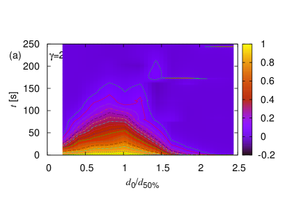
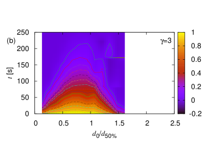
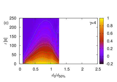
Figure 4: (Color online) Finite-size scaling showing the change in the form of the time autocorrelation function $G(t)$ with varying gamma: (a) $\gamma=2$, (b) $\gamma=3$, (c) $\gamma=4$. Simulations are carried out using the linear trajectory weighting. The tree had 20 levels, and $\alpha=3\times 10^{-4}$ and $\tau=0.1$. The lines are contours on $G(t)$. On increasing $\gamma$, the timescale can be seen to increase, with the shape of the contours becoming less rounded.

Figure 5: The curves of integrated correlation time become more sharply peaked on increasing $\gamma$. $\tau=0.1$, $\alpha=3\times 10^{-4}$. Curves are shown for various $\gamma$ and linear trajectory weighting. The tree had 20 levels, and $\alpha=3\times 10^{-4}$ and $\tau=0.1$. $d_{\max}$ is the maximum in the integrated correlation time curve.

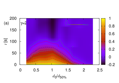
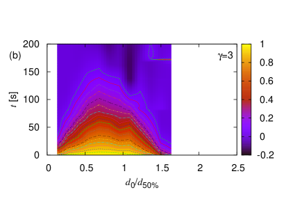
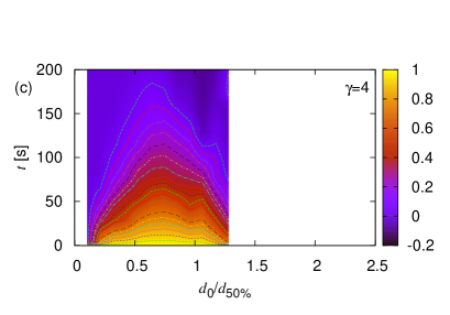
Figure 6: (Color online) Change in time autocorrelation function $G(t)$ with varying gamma: (a) $\gamma=2$, (b) $\gamma=3$, (c) $\gamma=4$. Simulations are carried out using the step function trajectory weighting. The tree had 20 levels, and $\alpha=3\times 10^{-4}$ and $\tau=0.1$. The time correlations become significantly longer and the peak in the contours becomes rapidly sharper as $\gamma$ increases.

A key question in this article is whether there is crossover or transition between the dilute and dense limits. In a non-equilibrium system at criticality, the timescale associated with fluctuations would diverge (in this case, the length of time that an additional embolus added to the system contributes to an overall increase in the level of obstruction). However, if there is a crossover, then while there could be increase in the timescale of correlations, no divergence would be seen. The appropriate measure of such fluctuations is the time autocorrelation function, which is computed from the expression,

$$G(t)=\frac{\langle(p(t)-\bar{p})(p(0)-\bar{p})\rangle}{\langle(p(0)-\bar{p})^{2}\rangle}$$ (15)

and the time correlation function according to,

$$\Gamma(t)=\frac{1}{N_{0}}\sum_{i=1}^{N_{0}}\langle(p_{i}(t)-\bar{p})(p_{i}(0)-\bar{p})\rangle,$$ (16)

where $p_{i}(t)=1$ if end node $i$ is blocked at time $t$ and $p_{i}(t)=0$ otherwise.

In a critical system, $\Gamma(t)$ should have the form,

$$\Gamma(t)\propto\frac{1}{t^{y}}e^{-t/\zeta}$$ (17)

where $y$ is a constant, and $\zeta$ is the correlation time. If $G(t)$ is positive at all times (i.e. there is no anticorrelation) it is possible to estimate the correlation time by summing (integrating) over the autocorrelation function, $\zeta\approx\Delta t\sum_{n=0}^{\infty}G(n\Delta t)$ (this measure is commonly known as the integrated correlation time).

To examine the existence of a phase transition, it is necessary of investigate the behavior of the system as the size is increased (note that the finite size scaling of the order parameter is discussed in the next section). The correct way of increasing the effective size of the system is unconventional. It is necessary to make the size difference between vessels smaller, which means that the emboli interact with more levels as they dissolve . This can be done by increasing $\gamma$, since the difference in vessel sizes between levels is $2^{1/\gamma}-1$. Fig. 4 shows the change in time autocorrelation function $G(t)$ with varying $\gamma$, when the linear trajectory weighting is used. So that the simulations with different $\gamma$ can be compared, we use the dimensionless parameter $d_{0}/d_{50\%}$. The size $d_{50\%}$ corresponds to half of end nodes receiving no flow. We note that $d_{50\%}$ is approximately proportional to $\gamma$. A distinct change in the shape of the contours can be seen, with the time scale increasing most rapidly towards the center of the graph as $\gamma$ is increased. This can be examined in the context of the integrated correlation time.

Figure 5 shows Monte Carlo results for the integrated correlation time. Increase in $\gamma$ has an effect on the correlation time consistent with a phase transition, with the hump associated with the maximum of the curve becoming more defined, and moving closer to the form consistent with a divergence, and thus a phase transition, for large $\gamma$. Time and memory constraints limit the maximum size of the tree, so we have been unable to examine systems with $\gamma>4$.

Finally, the time auto-correlators are examined in the context of the step function weighting of embolus trajectory, with the results shown in Fig. 6. Again an increase in the timescale is seen on increasing $\gamma$, with qualitatively similar changes in the form of the graphs to those seen for the linear weighting scheme. In the case of the step function weighting, there are regions of anti-correlation, so the integrated correlation time can not be used to examine the timescale. Since there is evidence of a phase transition at large $\gamma$, it remains to find a plausible candidate for the order parameter.

V Space-time plots and order parameter

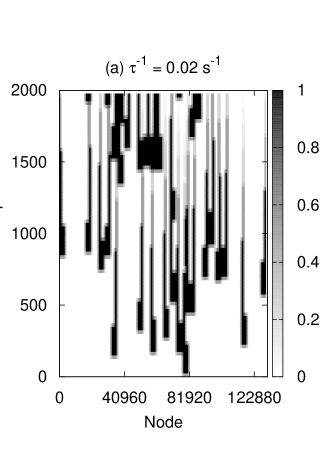
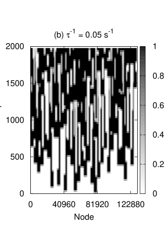
Figure 7: Space-time plot showing flow in end arterioles in the model with $b=1$ (linear weighting model). The tree consists of $M_{\ell}=18$ levels with $\gamma=2$, $d_{0}=0.2$mm and $\alpha=10^{-4}$mms^-1. Fully blocked regions are shown in black, and free flow in white. Panel (a) shows the dilute limit where emboli have available space to avoid each other. In contrast (b) shows the dense limit, where emboli are forced to occupy the same trees since there is no remaining space. This indicates that overlapped blockages are relevant to the phase transition.

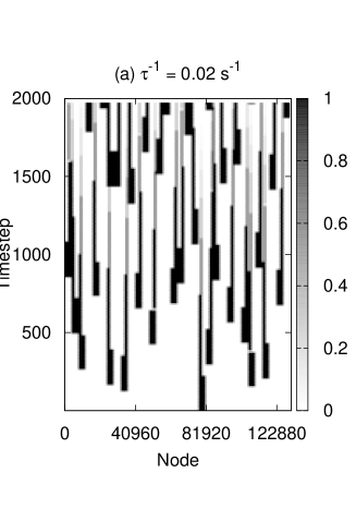
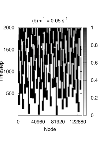
Figure 8: As Fig. 7 but with $b\rightarrow\infty$ (step function trajectory weighting). The emboli become more evenly spaced in the tree, leading to a state that appears to be more ordered in space.

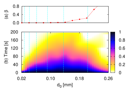
Figure 9: (color online) Main panel: Time correlator as $d_{0}$ is changed. $M_{\ell}=20$, $\gamma=1.736$, $\tau^{-1}=0.1$s^-1 and $\alpha=3\times 10^{-4}$mm/s. Errors on individual points are approximately 3% of the $t=0$ value (3 standard deviations). The timescale is significantly increased close to the transition. Top panel: The overlap between flow shadows shows how the significant increase in timescale is associated with the onset of order.

Figure 10: (a) Overlap parameter, $\beta$ showing a second-order transition. The hump features are related to partially occupied levels. (b) Percentage of blocked states and limiting behavior. The vertical lines indicate the sizes of nodes at each level of the tree. $M_{\ell}=18$ with $\gamma=2$, $\tau^{-1}=0.1$s^-1 and $\alpha=3\times 10^{-4}$mm/s. (Inset: $M_{\ell}=20$, $\gamma=2.151$, $\tau^{-1}=0.1$s^-1 and $\alpha=10^{-4}$mm/s.) Where no error bars are visible, they are smaller than the markers. For these parameters, overlap between blockages suddenly increases at $d_{0}=0.18$mm in a second order transition. The percentage of blocked end nodes is always non-zero.

Figure 11: Blockage and overlap parameter as $\gamma$ is varied to carry out the finite size scaling. Simulations are carried out using both step function and linear trajectory weighting. The tree had 20 levels, $\alpha=3\times 10^{-4}$ and $\tau=0.1$. Some of the small $d_{0}$ points are missing on the plots relating to the step function trajectory weighting, since $\beta=0$. As $\gamma$ is increased, the values of $\beta$ decrease for $d_{0}<d_{50\%}$ and $\beta$ increases for initial embolus sizes $d_{0}>d_{50\%}$. Scaling of this type is consistent with a phase transition.

In order to examine how the model changes on going through the transition, we followed the motion of emboli through the model arterial tree for specific realizations of the embolization. Fig. 7 displays spacetime plots showing which capillaries (end nodes) do not receive flow during a single run when the linear flow weighting scheme was used. Panel (a) shows the dilute limit where emboli are able to avoid each other. Each ‘wedge-like’ pattern represents the lifetime of an embolus, which initially blocks a large number of nodes, then dissolves and moves to block a smaller node. There is no clear spatial ordering between the emboli. In contrast (b) shows the dense limit, where space limitations force emboli to cast ‘flow shadows’ on the same arterioles: emboli in different flow levels cause the same end nodes to lose flow. This indicates that overlapping blockages could be important in the transition.

It is also of interest to see what differences the step function weighting scheme makes to the distribution of emboli in the vasculature. Fig. 8 shows spacetime plots for $b\rightarrow\infty$ (step function trajectory weighting) with model parameters that are otherwise the same as for Fig. 7. The effect of the step function weighting is to strongly redirect the emboli away from blocked vessels. Thus the emboli become more evenly spaced in the tree, leading to a state that appears to be more ordered in space. Again, when large numbers of emboli are present in the network, the tree becomes sufficiently populated that emboli can no longer avoid each other, so the flow shadows from blockages overlap.

The spacetime plots in Figs. 7 and 8 indicate that the main change in the state of the model on increasing embolus size is the overlap between blockages. Therefore, we suggest that the following measure of the overlap between flow shadows, $\beta$, may act as an order parameter,

$$\beta=\langle\sum_{i\neq j}n_{i}n_{j}\rangle,$$ (18)

where $n_{i}=1$ if an embolus in level $i$ stops flow in the end arterioles at level $0$.

If $\beta$ were the order parameter, then the timescale associated with correlations would peak at the embolus size where the order parameter becomes finite. To investigate this, Fig. 9 shows Monte Carlo results revealing how the time autocorrelation function changes with initial embolus size (bottom panel) alongside the overlap parameter (top panel). The hump features in both $\beta$ and the time autocorrelation function are related to prefactors introduced when the largest emboli do not have the same size as a node. The timescale associated with correlations is largest when $d_{0}=0.14$mm, corresponding to the embolus size where overlap of flow shadows becomes significant. This is a strong indicator that $\beta$ is the order parameter.

We also address whether the proportion of blockages could be the order parameter, rather than the overlap of blockages. Fig. 10(a) shows numerical results for the overlap of blockages, $\beta$. For these parameters, overlap between co-existing blockages suddenly increases at $d_{0}=0.18$mm. In contrast, panel (b) shows that the percentage of blocked end nodes is always non-zero and is unlikely to be the order parameter of the non-equilibrium transition. The limiting behaviors are also displayed on panel (b) for completeness and agree with the Monte Carlo results. Generally, the steady state approximation becomes more appropriate as system size increases.

We complete this section by examining the blockage $p$ and overlap parameter $\beta$ as $\gamma$ is varied to carry out the finite size scaling, as shown in Fig. 11. We reiterate that the finite size scaling associated with this problem is unusual. Increasing $\gamma$ means that the emboli (which dissolve linearly with time) interact with increasing numbers of nodes. As $\gamma$ is increased, the change in the proportion of blocked end nodes on increasing $d_{0}/d_{50\%}$ is more abrupt. As we showed in the last section, the timescale associated with fluctuations becomes more sharply peaked when $\gamma$ increases. We also show the overlap parameter $\beta$ on a logarithmic scale. $\beta$ changes over several orders of magnitude as $d_{0}$ is changed. As $\gamma$ is increased, the values of $\beta$ decrease for $d_{0}<d_{50\%}$ and $\beta$ increases for initial embolus sizes $d_{0}>d_{50\%}$. Scaling of this type is consistent with a phase transition, and can be seen for both the step-function and linear trajectory weighting.

VI Summary and conclusions

We have discussed the statistical physics of cerebral embolization leading to stroke based on analysis of a minimal model of particles moving through the cerebral arteries. We investigated whether the onset of stroke is associated with a gradual crossover or a phase transition. Our model is non-trivial since the trajectories of emboli are weighted away from blocked arterioles, generating an effective interaction. Examination of the time correlator showed that the timescale of fluctuations increases significantly at a critical value, consistent with a phase transition. Finite size scaling adds further weight to this view. We note that finite size scaling shows that the phase transition strictly occurs when the bifurcation exponent $\gamma=\infty$, since for reasons discussed earlier in this article the system has a finite size when $\gamma$ is finite. Thus crossover behavior is found when $\gamma$ is finite, but is controlled by the large $\gamma$ phase transition. The order parameter was identified as the overlap of blockage flow shadows defined by $\beta=\langle\sum_{i\neq j}n_{i}n_{j}\rangle$. Our model shows that the onset of stroke can be thought of as driven by non-equilibrium critical behavior. Further modeling incorporating increasingly realistic embolus parameters and anatomy promises to aid our understanding of embolic stroke, cerebrovascular disease and perfusion injury.

We briefly summarize the differences and similarities between our work and the directed percolation problem Hinrichsen (2000). In the directed percolation problem, flow stops when the number of broken bonds reaches a critical value corresponding to an absence of routes from source to exit. There are some crucial differences between the standard directed percolation problem, and the one described here. The first major difference is that the liquid is carrying particles which can break bonds and move the system closer to the percolation threshold. The second difference is that flow routes re-form after a characteristic time as emboli dissolve. The third crucial difference is that the properties of the tree downstream from the input influence the direction in which bond-breaking particles are carried, so blockages are not randomly distributed. In this respect, our model represents an entirely new type of percolation problem.

The existence of a phase transition in the flow could be of clinical relevance (although we add the caveat that our results should not be directly applied to medical treatment at the current time). Not only would an organized state have more blocked nodes than a randomly ordered positioning of emboli in the cerebral arteries, but also the increased time scales associated with fluctuations close to the transition would tend to increase the risk of brain damage during embolization.

Further work will be carried out to improve the model. For example, all branchings are currently symmetric, whereas asymmetric branchings are more common in the vasculature, so an algorithm will be developed to construct more realistic trees. Also, we are currently carrying out detailed laboratory tests of the paths of emboli at single asymmetric bifurcations, and in a silica replica of the major cerebral arteries, and these results will guide realistic development of the computational model.

VII Acknowledgments

JPH acknowledges useful discussions with Richard Blythe, Michael Wilkinson and Andrey Umerski. EMLC acknowledges the support of the British Heart Foundation.

References

- Lopez and Murray (1998) A. D. Lopez and C. J. L. Murray, Nature Medicine 4, 1241 (1998).
- Mackinnon et al. (2005) A. D. Mackinnon, R. Aaslid, and H. S. Markus, Stroke 36, 1726 (2005).
- Moody et al. (1990) D. M. Moody, M. E. Bell, V. R. Challa, W. E. Johnston, and D. S. Prough, Ann. Neurol. 28, 477 (1990).
- Bucerius et al. (2003) J. Bucerius, J. F. Gunnert, M. A. Borger, T. Walther, N. Doll, J. F. Onnasch, S. Metz, V. Falk, and F. W. Mohr, Ann. Thorac. Surg. 75, 472 (2003).
- Chung et al. (2007) E. M. L. Chung, J. P. Hague, and D. H. Evans, Phys. Med. Biol. 52, 7153 (2007).
- Cassot et al. (2006) F. Cassot, F. Lauwers, C. Fouard, S. Prohaska, and V. Lauwers-Cances, Microcirculation 13, 1 (2006).
- Karshafian et al. (2003) R. Karshafian, P. N. Burns, and M. R. Henkelman, Phys. Med. Biol. 48, 3225 (2003).
- Murray (1926) C. D. Murray, Proc. Natl. Acad. Sci. USA 12, 207 (1926).
- West et al. (1997) G. B. West, J. H. Brown, and B. J. Enquist, Science 276, 122 (1997).
- Zamir (1999) M. Zamir, Journal of Theoretical Biology 197, 517 (1999).
- Cieslicki and Ciesla (2005) K. Cieslicki and D. Ciesla, Journal of Biomechanics 38, 2302 (2005).
- Levick (2003) J. R. Levick, An introduction to Cardiovascular Physiology (Arnold, London, 2003), chap. 8.
- Bushi et al. (2005) D. Bushi, Y. Grad, S. Einav, O. Yodfat, and B. Nishri, Stroke 36, 2696 (2005).
- Hinrichsen (2000) H. Hinrichsen, Adv. Phys. 49, 815 (2000).