Resummation approach in Fractional APT:
How many loops do we need to calculate?

Abstract

We give short introduction to the Analytic Perturbation Theory (APT) [1] in QCD, describe its problems and suggest as a tool for their resolution the Fractional APT (FAPT) [2, 3]. We also describe shortly how to treat heavy-quark thresholds in FAPT and then show how to resum perturbative series in both the one-loop APT and FAPT. As applications of this approach we consider the Higgs boson decay $H^{0}\to b\bar{b}$, the Adler function $D(Q^{2})$ and the ratio $R(s)$ in the $N_{f}=4$ region. Our conclusion is that there is no need to calculate higher-order coefficients $d_{n\geq 5}$ if we are interested in the accuracy of the order of 1%.

1 Basics of APT in QCD

In the standard QCD Perturbation Theory (PT) we know that the Renormalization Group (RG) equation $da_{s}[L]/dL=-a_{s}^{2}-\ldots$ for the effective coupling $\alpha_{s}(Q^{2})=a_{s}[L]/\beta_{f}$ with $L=\ln(Q^{2}/\Lambda^{2})$, $\beta_{f}=b_{0}(N_{f})/(4\pi)=(11-2N_{f}/3)/(4\pi)$. Then the one-loop solution generates Landau pole singularity, $a_{s}[L]=1/L$.

In the Analytic Perturbation Theory (APT) we have different effective couplings in Minkowskian (Radyushkin [4], and Krasnikov and Pivovarov [5]) and Euclidean (Shirkov and Solovtsov [1]) regions. In Euclidean domain, $\displaystyle-q^{2}=Q^{2}$, $\displaystyle L=\ln Q^{2}/\Lambda^{2}$, APT generates the following set of images for the effective coupling and its $n$-th powers, $\displaystyle\left\{{\mathcal{A}}_{n}[L]\right\}_{n\in\mathbb{N}}$, whereas in Minkowskian domain, $\displaystyle q^{2}=s$, $\displaystyle L_{s}=\ln s/\Lambda^{2}$, it generates another set, $\displaystyle\left\{{\mathfrak{A}}_{n}[L_{s}]\right\}_{n\in\mathbb{N}}$. APT is based on the RG and causality that guaranties standard perturbative UV asymptotics and spectral properties. Power series $\sum_{m}d_{m}a_{s}^{m}[L]$ transforms into non-power series $\sum_{m}d_{m}{\mathcal{A}}_{m}[L]$ in APT.

By the analytization in APT for an observable $f(Q^{2})$ we mean the “Källen–Lehman” representation

$$\left[f(Q^{2})\right]_{\text{an}}=\int_{0}^{\infty}\!\frac{\rho_{f}(\sigma)}{\sigma+Q^{2}-i\epsilon}\,d\sigma~{}~{}\text{with}~{}~{}\rho_{f}(\sigma)=\frac{1}{\pi}\,\textbf{Im}\,\big{[}f(-\sigma)\big{]}\,.$$ (1)

Then in the one-loop approximation (note pole remover $(e^{L}-1)^{-1}$ in (2a))

$$\mathcal{A}_{1}[L] = \int_{0}^{\infty}\!\frac{\rho(\sigma)}{\sigma+Q^{2}}\,d\sigma\ =\ \frac{1}{L}-\frac{1}{e^{L}-1}\,,~{}$$ (2a)

$${\mathfrak{A}}_{1}[L_{s}] = \int_{s}^{\infty}\!\frac{\rho(\sigma)}{\sigma}\,d\sigma\ =\ \frac{1}{\pi}\,\arccos\frac{L_{s}}{\sqrt{\pi^{2}+L_{s}^{2}}}\,,~{}$$ (2b)

whereas analytic images of the higher powers ($n\geq 2,n\in\mathbb{N}$) are:

$${\mathcal{A}_{n}[L]\choose\mathfrak{A}_{n}[L_{s}]} = \frac{1}{(n-1)!}\left(-\frac{d}{dL}\right)^{n-1}{\mathcal{A}_{1}[L]\choose\mathfrak{A}_{1}[L_{s}]}\,.$$ (3)

In the standard QCD PT we have also:
(i) the factorization procedure in QCD that gives rise to the appearance of logarithmic factors of the type: $a_{s}^{\nu}[L]\,L$; 
(ii) the RG evolution that generates evolution factors of the type: $B(Q^{2})=\left[Z(Q^{2})/Z(\mu^{2})\right]$ $B(\mu^{2})$, which reduce in the one-loop approximation to $Z(Q^{2})\sim a_{s}^{\nu}[L]$ with $\nu=\gamma_{0}/(2b_{0})$ being a fractional number.
All these means we need to construct analytic images of new functions: $\displaystyle a_{s}^{\nu},~{}a_{s}^{\nu}\,L^{m},\ldots$ .

In the one-loop approximation using recursive relation (2) we can obtain explicit expressions for ${\mathcal{A}}_{\nu}[L]$ and ${\mathfrak{A}}_{\nu}[L]$:

$${\mathcal{A}}_{\nu}[L]=\frac{1}{L^{\nu}}-\frac{F(e^{-L},1-\nu)}{\Gamma(\nu)}\,;\quad{\mathfrak{A}}_{\nu}[L]=\frac{\text{sin}\left[(\nu-1)\arccos\left(L/\sqrt{\pi^{2}+L^{2}}\right)\right]}{\pi(\nu-1)\left(\pi^{2}+L^{2}\right)^{(\nu-1)/2}}\,.~{}$$ (4)

Here $F(z,\nu)$ is reduced Lerch transcendental function, which is an analytic function in $\nu$. Interesting to note that ${\mathcal{A}}_{\nu}[L]$ appears to be an entire function in $\nu$, whereas ${\mathfrak{A}}_{\nu}[L]$ is determined completely in terms of elementary functions. They have very interesting properties, which we discussed extensively in our previous papers [2, 7]. Here we only display graphics of ${\mathcal{A}}_{\nu}[L]$ and ${\mathfrak{A}}_{\nu}[L]$ in Fig. 1: one can see here a kind of distorting mirror on both panels.

   

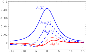
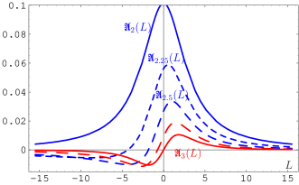
Figure 1: Graphics of ${\mathcal{A}}_{\nu}[L]$ (left panel) and ${\mathfrak{A}}_{\nu}[L]$ (right panel) for fractional $\nu\in\left[2,3\right]$.

Construction of FAPT with fixed number of quark flavors, $N_{f}$, is a two-step procedure: we start with the perturbative result $\left[a_{s}(Q^{2})\right]^{\nu}$, generate the spectral density $\rho_{\nu}(\sigma)$ using Eq. (1), and then obtain analytic couplings ${\mathcal{A}}_{\nu}[L]$ and ${\mathfrak{A}}_{\nu}[L]$ via Eqs. (2). Here $N_{f}$ is fixed and factorized out. We can proceed in the same manner for $N_{f}$-dependent quantities: $\left[\alpha_{s}(Q^{2};N_{f})\right]^{\nu}$ $\Rightarrow$ $\bar{\rho}_{\nu}(\sigma;N_{f})=\bar{\rho}_{\nu}[L_{\sigma};N_{f}]\equiv\rho_{\nu}(\sigma)/\beta_{f}^{\nu}$ $\Rightarrow$ $\bar{\mathcal{A}}_{\nu}[L;N_{f}]$ and $\bar{\mathfrak{A}}_{\nu}[L;N_{f}]$ — here $N_{f}$ is fixed, but not factorized out.

Global version of FAPT, which takes into account heavy-quark thresholds, is constructed along the same lines but starting from global perturbative coupling $\left[\alpha_{s}^{\,\text{\tiny glob}}(Q^{2})\right]^{\nu}$, being a continuous function of $Q^{2}$ due to choosing different values of QCD scales $\Lambda_{f}$, corresponding to different values of $N_{f}$. We illustrate here the case of only one heavy-quark threshold at $s=m_{4}^{2}$, corresponding to the transition $N_{f}=3\to N_{f}=4$. Then we obtain the discontinuous spectral density

$$\rho_{n}^{\text{\tiny glob}}(\sigma)=\rho_{n}^{\text{\tiny glob}}[L_{\sigma}]=\theta\left(L_{\sigma}<L_{4}\right)\,\bar{\rho}_{n}\left[L_{\sigma};3\right]+\theta\left(L_{4}\leq L_{\sigma}\right)\,\bar{\rho}_{n}\left[L_{\sigma}+\lambda_{4};4\right]\,,~{}~{}~{}$$ (5)

with $L_{\sigma}\equiv\ln\left(\sigma/\Lambda_{3}^{2}\right)$, $L_{f}\equiv\ln\left(m_{f}^{2}/\Lambda_{3}^{2}\right)$ and $\lambda_{f}\equiv\ln\left(\Lambda_{3}^{2}/\Lambda_{f}^{2}\right)$ for $f=4$, which is expressed in terms of fixed-flavor spectral densities with 3 and 4 flavors, $\bar{\rho}_{n}[L;3]$ and $\bar{\rho}_{n}[L+\lambda_{4};4]$. However it generates the continuous Minkowskian coupling

$${\mathfrak{A}}_{\nu}^{\text{\tiny glob}}[L_{s}]\! \!=\! \!\theta\left(L_{s}\!<\!L_{4}\right)\Bigl{(}\bar{{\mathfrak{A}}}_{\nu}[L_{s};3]-\bar{{\mathfrak{A}}}_{\nu}[L_{4};3]+\bar{{\mathfrak{A}}}_{\nu}[L_{4}+\lambda_{4};4]\Bigr{)}$$ (6)

$$\!+\! \!\theta\left(L_{4}\!\leq\!L_{s}\right)\,\bar{{\mathfrak{A}}}_{\nu}[L_{s}+\lambda_{4};4]\,.$$

and the analytic Euclidean coupling (for more detail see in [7])

$${\cal A}_{\nu}^{\text{\tiny glob}}[L] = \bar{{\cal A}}_{\nu}[L+\lambda_{4};4]+\int\limits_{-\infty}^{L_{4}}\!\frac{\bar{\rho}_{\nu}[L_{\sigma};3]-\bar{\rho}_{\nu}[L_{\sigma}+\lambda_{4};4]}{1+e^{L-L_{\sigma}}}\,dL_{\sigma}\,.$$ (7)

2 Resummation in the one-loop APT and FAPT

We consider now the perturbative expansion of a typical physical quantity, like the Adler function and the ratio $R$, in the one-loop APT

$${\mathcal{D}[L]\choose\mathcal{R}[L]}=d_{0}+\sum_{n=1}^{\infty}d_{n}\,{\mathcal{A}_{n}[L]\choose\mathfrak{A}_{n}[L]}\,.$$ (8)

We suggest that there exist the generating function $P(t)$ for coefficients $\tilde{d}_{n}=d_{n}/d_{1}$:

$$\tilde{d}_{n}=\int_{0}^{\infty}\!\!P(t)\,t^{n-1}dt~{}~{}~{}\text{with}~{}~{}~{}\int_{0}^{\infty}\!\!P(t)\,dt=1\,.$$ (9)

To shorten our formulae, we use the following notation $\langle\langle{f(t)}\rangle\rangle_{P(t)}\equiv\int_{0}^{\infty}\!\!f(t)P(t)dt$. Then coefficients $d_{n}=d_{1}\,\langle\langle{t^{n-1}}{P(t)}$ and as has been shown in [8] we have the exact result for the sum in (8)

$${\mathcal{D}[L]\choose\mathcal{R}[L]}=d_{0}+d_{1}\,{\langle\langle{\mathcal{A}_{1}[L-t]}\rangle\rangle_{P(t)}\choose\langle\langle{\mathfrak{A}_{1}[L-t]}\rangle\rangle_{P(t)}}\,.$$ (10)

The integral in variable $t$ here has a rigorous meaning, ensured by the finiteness of the couplings $\mathcal{A}_{1}[t]\leq 1$ and $\mathfrak{A}_{1}[t]\leq 1$ and fast fall-off of the generating function $P(t)$.

In our previous publications [7, 9] we have constructed generalizations of these results, first, to the case of the global APT, when heavy-quark thresholds are taken into account. Then one starts with the series of the type (8), where $\mathcal{A}_{n}[L]$ or $\mathfrak{A}_{n}[L]$ are substituted by their global analogs, $\mathcal{A}_{n}^{\text{\tiny glob}}[L]$ or $\mathfrak{A}_{n}^{\text{\tiny glob}}[L]$ (note that due to different normalizations of global couplings, $\mathcal{A}_{n}^{\text{\tiny glob}}[L]\simeq\mathcal{A}_{n}[L]/\beta_{f}$, the coefficients $d_{n}$ should be also changed). The most simple generalization of the summation result appears in Minkowski domain:

$$\mathcal{R}^{\text{\tiny glob}}[L]=d_{0}\!\! \!+\! \!\!d_{1}\langle\langle{\theta(L\!<\!L_{4})\left[\Delta_{4}\bar{\mathfrak{A}}_{1}[t]+\bar{\mathfrak{A}}_{1}\!\Big{[}L\!-\!\frac{t}{\beta_{3}};3\Big{]}\right]}\rangle\rangle_{P(t)}$$ (11)

$$\!+\! \!\!d_{1}\langle\langle{\theta(L\!\geq\!L_{4})\bar{\mathfrak{A}}_{1}\!\Big{[}L\!+\!\lambda_{4}-\!\frac{t}{\beta_{4}};4\Big{]}}\rangle\rangle_{P(t)}\,;~{}~{}~{}$$

where $\Delta_{4}\bar{\mathfrak{A}}_{\nu}[t]\equiv\bar{\mathfrak{A}}_{\nu}\!\Big{[}L_{4}+\lambda_{4}-t/\beta_{4};4\Big{]}-\bar{\mathfrak{A}}_{\nu}\!\Big{[}L_{3}-t/\beta_{3};3\Big{]}$.

The second generalization has been obtained for the case of the global FAPT. Then the starting point is the series of the type $\sum_{n=0}^{\infty}d_{n}\,\mathfrak{A}_{n+\nu}^{\text{\tiny glob}}[L]$ and the result of summation is a complete analog of Eq. (11) with substitutions

$$P(t)\Rightarrow P_{\nu}(t)=\int_{0}^{1}\!P\left(\frac{t}{1-x}\right)\frac{\nu\,x^{\nu-1}dx}{1-x}\,,$$ (12)

$d_{0}\Rightarrow d_{0}\,\bar{\mathfrak{A}}_{\nu}[L]$, $\bar{\mathfrak{A}}_{1}[L-t]\Rightarrow\bar{\mathfrak{A}}_{1+\nu}[L-t]$, and $\Delta_{4}\bar{\mathfrak{A}}_{1}[t]\Rightarrow\Delta_{4}\bar{\mathfrak{A}}_{1+\nu}[t]$. Needless to say that all needed formulas have been also obtained in parallel for the Euclidean case.

3 Applications to Higgs boson decay and Adler function

First, we analyze the Higgs boson decay to a $\bar{b}b$ pair. Here we have for the decay width

$$\Gamma(\text{H}\to b\bar{b})=\frac{G_{F}}{4\sqrt{2}\pi}\,M_{H}\,\widetilde{R}_{\text{\tiny S}}(M_{H}^{2})~{}~{}~{}\text{with}~{}~{}~{}\widetilde{R}_{\text{\tiny S}}(M_{H}^{2})\equiv m^{2}_{b}(M_{H}^{2})\,R_{\text{\tiny S}}(M_{H}^{2})$$ (13)

and $R_{\text{\tiny S}}(s)$ is the $R$-ratio for the scalar correlator, see for details in [2, 10]. In the one-loop FAPT this generates the following non-power expansion:

$$\widetilde{\mathcal{R}}_{\text{\tiny S}}[L]=3\,\hat{m}_{(1)}^{2}\,\Bigg{\{}\mathfrak{A}_{\nu_{0}}^{\text{\tiny glob}}[L]+d_{1}^{\text{\,\tiny S}}\,\sum_{n\geq 1}\frac{\tilde{d}_{n}^{\text{\,\tiny S}}}{\pi^{n}}\,\mathfrak{A}_{n+\nu_{0}}^{\text{\tiny glob}}[L]\Bigg{\}}\,,$$ (14)

where $\hat{m}_{(1)}^{2}$ is the renormalization-group invariant of the one-loop $m^{2}_{b}(\mu^{2})$ evolution $m_{b}^{2}(Q^{2})=\hat{m}_{(1)}^{2}\,\alpha_{s}^{\nu_{0}}(Q^{2})$ with $\nu_{0}=2\gamma_{0}/b_{0}(5)=1.04$ and $\gamma_{0}$ is the quark-mass anomalous dimension (for a discussion — see in [11]).

We take for the generating function $P(t)$ the Lipatov-like model of [9, 12] with $\left\{c=2.4,~{}\beta=-0.52\right\}$

$$\tilde{d}_{n}^{\text{\,\tiny S}}=c^{n-1}\frac{\Gamma(n+1)+\beta\,\Gamma(n)}{1+\beta}\,;\quad P_{\text{\tiny S}}(t)=\frac{(t/c)+\beta}{c\,(1+\beta)}\,e^{-{t/c}}\,.$$ (15)

It gives a very good prediction for $\tilde{d}_{n}^{\text{\,\tiny S}}$ with $n=2,3,4$, calculated in the QCD PT [10]: $7.50$, $61.1$, and $625$ in comparison with $7.42$, $62.3$, and $620$. Then we apply FAPT resummation technique to estimate how good is FAPT in approximating the whole sum $\widetilde{\mathcal{R}}_{\text{\tiny S}}[L]$ in the range $L\in[11,13.8]$ which corresponds to the range $M_{H}\in[60,170]$ GeV² with $\Lambda^{N_{f}=3}_{\text{QCD}}=172$ MeV and ${\mathfrak{A}}^{\text{\tiny glob}}_{1}(m_{Z}^{2})=0.120$. In this range we have ($L_{6}=\ln(m_{t}^{2}/\Lambda_{3}^{2})$)

$$\widetilde{\mathcal{R}}_{\text{\tiny S}}[L]=3\,\hat{m}_{(1)}^{2}\,\left\{{\mathfrak{A}}^{\text{\tiny glob}}_{\nu_{0}}[L]+\frac{d_{1}^{\text{\,\tiny S}}}{\pi}\,\langle\langle{\bar{\mathfrak{A}}_{1+\nu_{0}}\!\Big{[}L\!+\!\lambda_{5}\!-\!\frac{t}{\pi\beta_{5}};5\Big{]}\!+\!\Delta_{6}\bar{\mathfrak{A}}_{1+\nu_{0}}\left[\frac{t}{\pi}\right]}\rangle\rangle_{P_{\nu_{0}}^{\text{\,\tiny S}}}\right\}$$ (16)

with $P_{\nu_{0}}^{\text{\,\tiny S}}(t)$ defined via Eqs. (15) and (12). Now we analyze the accuracy of the truncated FAPT expressions

$$\widetilde{\mathcal{R}}_{\text{\tiny S}}[L;N] = 3\,\hat{m}_{(1)}^{2}\,\left[{\mathfrak{A}}_{\nu_{0}}^{\text{\tiny glob}}[L]+d_{1}^{\text{\,\tiny S}}\,\sum_{n=1}^{N}\frac{\tilde{d}_{n}^{\text{\,\tiny S}}}{\pi^{n}}\,{\mathfrak{A}}_{n+\nu_{0}}^{\text{\tiny glob}}[L]\right]$$ (17)

and compare them with the total sum $\widetilde{\mathcal{R}}_{\text{\tiny S}}[L]$ in Eq. (16) using relative errors $\Delta_{N}^{\text{S}}[L]=1-\widetilde{\mathcal{R}}_{\text{\tiny S}}[L;N]/\widetilde{\mathcal{R}}_{\text{\tiny S}}[L]$. In the left panel of Fig. 2 we show these errors for $N=2$, $N=3$, and $N=4$ in the analyzed range of $L\in[11,13.8]$. We see that already $\widetilde{\mathcal{R}}_{\text{\tiny S}}[L;2]$ gives accuracy of the order of 2.5%, whereas $\widetilde{\mathcal{R}}_{\text{\tiny S}}[L;3]$ of the order of 1%. That means that there is no need to calculate further corrections: at the level of accuracy of 1% it is quite enough to take into account only coefficients up to $d_{3}$. This conclusion is stable with respect to the variation of parameters of the model $P_{\text{\tiny S}}(t)$.

   

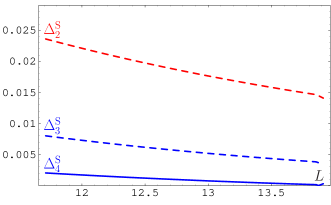
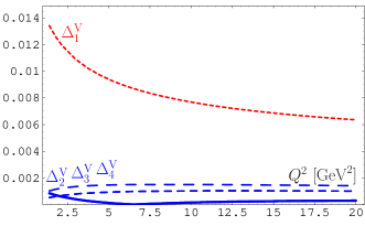
Figure 2: Left panel: The relative errors $\Delta^{\text{S}}_{N}[L]$, $N=2,3$ and $4$, of the truncated FAPT, Eq. (17), in comparison with the exact summation result, Eq. (16). Right panel: Analogous relative errors $\Delta^{\text{V}}_{N}(Q^{2})$, $N=1,\ldots,4$, for the case of vector Adler function (solid line is for $N=2$, dashed — for $N=3$, and long-dashed — for $N=4$).

Next, we analyze the Adler function of vector correlator. In the one-loop APT this generates the following non-power expansion:

$$\mathcal{D}_{\text{\tiny V}}[L]=1+d_{1}^{\text{\tiny V}}\,\sum_{n\geq 1}\frac{\tilde{d}_{n}^{\text{\tiny V}}}{\pi^{n}}\,\mathcal{A}_{n}^{\text{\tiny glob}}[L]\,,$$ (18)

Here we use another Lipatov-like model for perturbative coefficients in the $N_{f}=4$ region

$$\tilde{d}_{n}^{\text{\tiny V}}=c^{n-1}\,\frac{\beta^{n+1}-n}{\beta^{2}-1}\,\Gamma(n)\,;\quad P_{\text{\tiny V}}(t)=\frac{\beta\,e^{-t/c\beta}-(t/c)\,e^{-t/c}}{c\left(\beta^{2}-1\right)}$$ (19)

with $c=3.456$ and $\beta=1.325$, which gives a very good prediction for $\tilde{d}_{n}^{\text{\tiny V}}$ with $n=2,3,4$, calculated in the QCD PT [13]: $1.49$, $2.60$, and $27.5$ in comparison with $1.52$, $2.59$, and $27.4$. To estimate how good is APT in approximating the whole sum $\mathcal{D}_{\text{\tiny S}}[L]$, we apply APT resummation approach in the range $Q^{2}\in[1.5,20]$ GeV², corresponding to the $N_{f}=4$ value. Again we analyze the accuracy of the truncated APT expressions $\mathcal{D}_{\text{\tiny V}}[L;N]=1+d_{1}^{\text{\,\tiny V}}\,\sum_{n=1}^{N}\frac{\tilde{d}_{n}^{\text{\,\tiny V}}}{\pi^{n}}\,\mathcal{A}_{n}^{\text{\tiny glob}}[L]$ and compare them with the total sum $\mathcal{D}_{\text{\tiny V}}[L]$, obtained by resummation APT method, using relative errors $\Delta_{N}^{\text{V}}[L]=1-\mathcal{D}_{\text{\tiny V}}[L;N]/\mathcal{D}_{\text{\tiny V}}[L]$. In the right panel of Fig. 2 we show these errors for $N=1,\ldots,4$ in the analyzed range of $Q^{2}$. We see that already $\mathcal{D}_{\text{\tiny V}}(Q^{2};2)$ gives the accuracy of the order of 0.05%, whereas taking into account higher-order corrections only worsen the accuracy: $\mathcal{D}_{\text{\tiny V}}(Q^{2};3)$ provides the accuracy of the order of 0.1% and $\mathcal{D}_{\text{\tiny V}}(Q^{2};4)$ — of the order of 0.2%. That means that the NLO approximation gives the best result and after that the series starts to reveal its asymptotic character.

4 Conclusions

In this report we described the resummation approach in the global versions of the one-loop APT and FAPT and argued that it produces finite answers in both Euclidean and Minkowski regions, provided the generating function $P(t)$ of perturbative coefficients $d_{n}$ is known. In the case of the Higgs boson decay an accuracy of the order of 1% is reached at N³LO approximation, when term $d_{3}{\mathcal{A}}_{3}$ is taken into account, whereas for the Adler function $D(Q^{2})$ we have an accuracy of the order of $0.1$% already at N²LO (i.e., with taking into account $d_{2}{\mathcal{A}}_{2}$ term).

The main conclusion is: In order to achieve an accuracy of the order of 1% we do not need to calculate more than four loops and $d_{4}$ coefficients are needed only to estimate corresponding generating functions $P(t)$.

References

[1]
D. V. Shirkov and I. L. Solovtsov,
JINR Rapid Commun. 2 [76] (1996) 5;
Phys. Rev. Lett. 79 (1997) 1209;
Theor. Math. Phys. 150 (2007) 132.
[2]
A. P. Bakulev, S. V. Mikhailov, and N. G. Stefanis,
Phys. Rev. D72 (2005) 074014, 119908(E);
Phys. Rev. D75 (2007) 056005;
77 (2008) 079901(E).
[3]
A. P. Bakulev, A. I. Karanikas, and N. G. Stefanis,
Phys. Rev. D72 (2005) 074015.
[4]
A. V. Radyushkin,
JINR Rapid Commun. 78 (1996) 96;
[JINR Preprint, E2-82-159, 26 Febr. 1982;
arXiv: hep-ph/9907228].
[5]
N. V. Krasnikov and A. A. Pivovarov,
Phys. Lett. B116 (1982) 168.
[6]
A. I. Karanikas and N. G. Stefanis,
Phys. Lett. B504 (2001) 225;
B636, 330 (2006).
[7]
A. P. Bakulev
“Global Fractional Analytic Perturbation Theory in QCD
with Selected Applications”,
Arxiv:0805.0829 [to be published in
Physics of Particles and Nuclei].
[8]
S. V. Mikhailov,
JHEP 06 (2007) 009.
[9]
A. P. Bakulev and S. V. Mikhailov,
in Proc. Int. Seminar on Contemp.
Probl. of Part. Phys.,
dedicated to the memory of I. L. Sovtsov,
Dubna, Jan. 17–18, 2008.,
Eds. A. P. Bakulev et al.
(JINR, Dubna, 2008),
pp. 119–133 (arXiv:0803.3013 [hep-ph]).
[10]
P. A. Baikov, K. G. Chetyrkin, and J. H. Kühn,
Phys. Rev. Lett. 96 (2006) 012003.
[11]
A. L. Kataev and V. T. Kim,
in Proc. Int. Seminar on Contemp.
Probl. of Part. Phys.,
dedicated to the memory of I. L. Sovtsov,
Dubna, Jan. 17–18, 2003.,
Eds. A. P. Bakulev et al.
(JINR, Dubna, 2008),
pp. 167–182 (arXiv:0804.3992 [hep-ph]).
[12]
L. N. Lipatov,
Sov. Phys. JETP 45 (1977) 216.
[13]
P. A. Baikov, K. G. Chetyrkin, and J. H. Kuhn,
arXiv:0801.1821 [hep-ph].