Lattice models for non-Fermi liquid metals

Abstract

We present two $2D$ lattice models with non-Fermi liquid metallic phases. We show that the low energy physics of these models is exactly described by a Fermi sea of fractionalized quasiparticles coupled to a fluctuating $U(1)$ gauge field. In the first model, the underlying degrees of freedom are spin $1/2$ fermions. This model demonstrates that electrons can in principle give rise to non-Fermi liquid metallic phases. In the second model, the underlying degrees of freedom are spinless bosons. This model provides a concrete example of a (non-Fermi liquid) Bose metal. With little modification, it also gives an example of a critical $U(1)$ symmetric spin liquid.

I Introduction

One of the basic tenets of conventional solid state physics is that clean metals behave like Landau Fermi liquids at low energies. That is, they are characterized by a sharp Fermi surface and sharp electron-like Landau quasiparticles that are gapless at this surface. An extraordinarily diverse collection of materials can be understood using this simple framework.

However, a number of experimental discoveries in the last two decades have challenged our general description of metals as Landau Fermi liquids. The most striking example is perhaps the normal state of the cuprate superconductors. Breakdowns of Fermi liquid behavior have also been observed in a number of other situations, notably in the vicinity of a quantum critical point associated with the onset of magnetism in heavy electron materials. Coleman and Schofield (2005); v. Lohneysen et al. (2007); Gegenwart et al. (2008)

These and other experimental developments have strongly challenged the conventional view of metals. Indeed a number of fundamental questions have been brought into sharp focus. Do stable metallic phases of interacting electrons exist that are not Landau Fermi liquids? Does a metal need to have a sharp Fermi surface and/or sharp electron-like quasiparticles? A perhaps even more fundamental question is whether metallicity is dependent on Fermi statistics of the charge carriers. In other words, could a collection of bosonic charge carriers form a metallic ground state? The possibility of such a “Bose metal” has been discussed much in the literature but without adequate resolution. Das and Doniach (1999, 2001); Phillips and Dalidovich (2003)

A limited amount of theoretical progress has been made towards answering these questions. Much of this progress has come from slave particle treatments of various models of correlated electron or boson systems. As is well-known, this approach leads to a description of various phases of the strongly correlated system in terms of fractionalized variables that are coupled to emergent gauge fields. A number of non-Fermi liquid metallic phases of interacting electrons have been described within such slave particle gauge theories. Ioffe and Larkin (1989); Lee and Nagaosa (1992); Lee (1989); Kaul et al. (2007, 2008) It is also possible to construct slave particle descriptions of Bose metal phases of interacting bosons. Motrunich and Fisher (2007) These constructions strongly suggest that exotic non-Fermi liquid metallic phases of interacting electrons or bosons are possible, at least in principle.

However, the slave particle approach has some well known limitations. The most important of these is that it does not usually allow for a definitive statement about the ground state of any particular microscopic model. In practice this means that even though we may be able to construct a stable effective field theory for a non-Fermi liquid phase using slave particle variables, the approach does not allow us to identify microscopic models that get into such a phase.

In this paper, we address this problem of finding definite microscopic models that have non-Fermi liquid phases. We present two concrete lattice models of non-Fermi liquid metals where the non-Fermi liquid physics can be derived directly from the microscopic interactions. The first model, a “generalized Kondo lattice” model, is a two dimensional ($2D$) system of localized magnetic moments coupled to a separate band of conduction electrons. The second model, a Bose-Hubbard model, is a $2D$ lattice boson model with a ring exchange term. While neither model is physically realistic, their low energy physics is exactly described by fractionalized fermionic particles coupled to a fluctuating $U(1)$ gauge field. When the fractionalized excitations form a Fermi sea the result is a non-Fermi liquid metallic phase (modulo possible pairing instabilities at $T=0$). Ioffe and Larkin (1989); Lee and Nagaosa (1992); Lee (1989); Halperin et al. (1993); Polchinski (1994); Altshuler et al. (1994) The first model thus demonstrates that electrons can form non-Fermi liquid metallic phases, while the second model provides an example of a Bose metal - in fact a non-Fermi liquid Bose metal. With little modification, it also gives an example of a critical $U(1)$ symmetric spin liquid.

Our strategy for constructing and analyzing these models is very straightforward. The idea is to make use of recent constructions of exactly soluble lattice boson models with unusual low energy physics. In particular, we make use of boson models whose low energy excitations are fermionic quasiparticles coupled to an emergent $U(1)$ gauge field. Levin and Wen (2006, 2005) Previous work on these models focused on the case where the fermionic excitations were gapped and the system was insulating. Here, we simply modify the models so that the fermionic excitations become gapless and open up a Fermi surface. In this way, we construct a boson model with a (non-Fermi liquid) metallic phase. The construction of the fermion model is similar (and in some sense even easier since the fermionic quasiparticle excitations come for free).

We would like to mention that lattice models of (non-Fermi liquid) Bose metals have appeared previously in the literature. Levin and Wen (2006) The main contribution of this paper is that the models presented here are simple and can be understood with minimal background. In addition, we discuss their implications for non-Fermi liquid metallic phases, unlike previous work where the examples were simply mentioned in passing.

The paper is organized as follows. In section II, we present the “generalized Kondo lattice model” while in section III, we describe the boson model. In section IV, we summarize our results and conclude.

II Non-Fermi liquid metallic phase in a generalized Kondo lattice

The system we consider is a lattice of localized magnetic moments coupled to a separate band of conduction electrons through a generalized “Kondo lattice” Hamiltonian. The conduction electrons live on the sites of the square lattice while the local moments, which have spin $S$, live on the bonds. The Hamiltonian - a variant of Appendix B of LABEL:SVS0411 - is defined by

$$H = H_{t}+H_{K\perp}+H_{Kz}+H_{s}$$ (1)

$$H_{t} = -t\sum_{\langle rr^{\prime}\rangle}\left(c^{\dagger}_{r\alpha}c_{r^{\prime}\alpha}+h.c\right)-\mu\sum_{r}c^{\dagger}_{r}c_{r}$$

$$H_{K\perp} = J_{K}\sum_{\langle rr^{\prime}\rangle}\left[\left(c^{\dagger}_{r\uparrow}c_{r^{\prime}\downarrow}+c^{\dagger}_{r^{\prime}\uparrow}c_{r\downarrow}\right)S^{-}_{rr^{\prime}}+h.c\right]$$

$$H_{Kz} = J_{Kz}\sum_{r}(I^{z}_{r})^{2}$$

$$H_{s} = J_{\perp}\sum_{\langle\langle rr^{\prime}r^{\prime\prime}\rangle\rangle}\left(S^{+}_{rr^{\prime}}S^{-}_{r^{\prime}r^{\prime\prime}}+h.c\right)+J_{z}\sum_{\langle rr^{\prime}\rangle}\left(S^{z}_{rr^{\prime}}\right)^{2}$$

Here $c_{r\alpha}$ is the conduction electron destruction operator for site $r$ and spin $\alpha=\uparrow,\downarrow$, while $\vec{S}_{rr^{\prime}}$ is the local moment spin operator on the bond $\langle rr^{\prime}\rangle$. The operator $I^{z}_{r}$ in the $H_{Kz}$ term is defined by

$$I^{z}_{r}=c^{\dagger}_{r}\sigma_{z}c_{r}+\sum_{r^{\prime}\in r}S^{z}_{rr^{\prime}}$$ (2)

where $r^{\prime}\in r$ means that $r^{\prime}$ is a nearest neighbor of $r$. $I^{z}_{r}$ may be viewed as the total $z$-component of the spin associated with a cluster composed of a site $r$ and the four bonds surrounding it (see Fig. 1). Note that in defining this ‘cluster spin’ we weight the central electronic contribution twice as much as the contribution from each of the four local moments on the bonds. This ensures that the total $z$ component of the spin is simply proportional to the sum of $I^{z}_{r}$ over all clusters. Specifically

$$S^{z}_{tot}=\frac{1}{2}\sum_{r}I^{z}_{r}$$ (3)

Finally, in the last term $H_{s}$, the notation $\langle\langle rr^{\prime}r^{\prime\prime}\rangle\rangle$ refers to the bonds shown in dashed lines in Figure 1.

These terms can be interpreted as follows. The first term $H_{t}$ contains the usual electron kinetic energy and chemical potential terms. The second term $H_{K\perp}$ is a Kondo spin exchange between the $XY$ spin components of the local momenta and conduction electron systems. The structure of this term corresponds to an event where a conduction electron hops across a bond by flipping its spin along with an opposite spin flip of the local moment that resides on the bond. Clearly this term, as well as other the other terms described below, imply that the model only has symmetry under spin rotations about the $z$-axis of spin. The term $H_{Kz}$ with $J_{Kz}>0$ penalizes fluctuations that change the total spin of the cluster that defines the operator $I^{z}_{r}$. Finally, the term $H_{s}$ is an inter-moment exchange term. Putting this all together, the Hamiltonian (II) can be thought of as a generalized ‘Kondo-Heisenberg’ model with a global $U(1)$ spin symmetry associated with conservation of the $z$ component of spin, and a distinct global $U(1)$ associated with electric charge conservation.

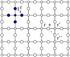
Figure 1: A picture of the cluster spin term $I^{z}_{r}=c^{\dagger}_{r}\sigma_{z}c_{r}+\sum_{r^{\prime}\in r}S^{z}_{rr^{\prime}}$ and the spin-spin coupling term $S^{+}_{rr^{\prime}}S^{-}_{r^{\prime}r^{\prime\prime}}$ in the generalized Kondo lattice model (II).

We now argue that when $t,J_{z},J_{\perp}\ll J_{Kz}$ and $J_{z}\ll J_{K},\frac{J_{\perp}^{2}}{J_{Kz}}$ and $|\mu|<4J_{K}$, this model realizes a non-Fermi liquid metallic phase (at least in the limit of large $S$). In order to simplify our analysis, we restrict to the case where the local moments have integer spin and we use a rotor description of this spin. Specifically we let

$$S^{+}_{rr^{\prime}} \sim e^{i\theta_{rr^{\prime}}}$$

$$S^{z}_{rr^{\prime}} = n_{rr^{\prime}}$$ (4)

where the phase $\theta_{rr^{\prime}}\in[0,2\pi]$ and ‘number’ $n_{rr^{\prime}}$ (which can take any integer value) are canonically conjugate:

$$[\theta_{rr^{\prime}},n_{rr^{\prime}}]=i$$ (5)

We will focus exclusively on the limit of large $J_{Kz}$ as this allows us to access the non-Fermi liquid metallic phase. In that limit we first diagonalize the $H_{Kz}$ term. The corresponding ground states satisfy

$$I^{z}_{r}=c^{\dagger}_{r}\sigma_{z}c_{r}+\sum_{r^{\prime}\in r}S^{z}_{rr^{\prime}}~{}~{}~{}=0$$ (6)

for each cluster $r$. This constraint leads to a highly degenerate manifold of ground states. This degeneracy will be split by the other terms in the Hamiltonian. Below we derive an effective Hamiltonian that lives entirely within this degenerate ground state manifold.

To that end we first make a familiar change of notation to recast the constraint (6) as the Gauss law constraint of a $U(1)$ gauge theory. We let $n_{rr^{\prime}}=\epsilon_{r}E_{rr^{\prime}},\theta_{rr^{\prime}}=\epsilon_{r}a_{rr^{\prime}}$ with $\epsilon_{r}=\pm 1$ on the A and B sublattices of the square lattice. Further, we define new fermion operators through

$$f_{r}=\left\{\begin{matrix}c_{r},&r\in A\\ \sigma^{x}c_{r},&r\in B\end{matrix}\right.$$ (7)

In this notation, the constraint (6) becomes

$$\vec{\nabla}\cdot\vec{E}+f^{\dagger}_{r}\sigma^{z}f_{r}=0$$ (8)

We may now derive an effective Hamiltonian that lives entirely in this constrained ground state subspace by degenerate perturbation theory. We initially set $t=0$ (and account for its effects later). To leading order in $\left(J_{z},J_{K},\mu,\frac{J_{\perp}^{2}}{J_{Kz}}\right)$, we find

$$H_{\text{eff}} = H_{f}+H_{a}$$ (9)

$$H_{f} = J_{K}\sum_{\langle rr^{\prime}\rangle}\left[f^{\dagger}_{r}e^{-ia_{rr^{\prime}}\sigma^{z}}f_{r^{\prime}}+h.c\right]$$

$$-\mu\sum_{r}f^{\dagger}_{r}f_{r}$$

$$H_{a} = -K\sum_{P}\cos\left(\vec{\nabla}\times\vec{a}\right)+J_{z}\sum_{\langle rr^{\prime}\rangle}\vec{E}_{rr^{\prime}}^{2}$$

where $K\sim\frac{J_{\perp}^{2}}{J_{Kz}}$ and the sum is taken over all plaquettes $P$ of the square lattice. Including the $t$ term gives a four fermion interaction between the $f$-fermions at $O(t^{2}/J_{Kz})$. As we do not expect this small short distance interaction to be important, we will ignore it in what follows.

The effective Hamiltonian $H_{\text{eff}}$ describes two species of fermions coupled to a fluctuating compact $U(1)$ gauge field with opposite gauge charges. The fermions carry physical charge $Q=e$, and spin $S^{z}=0$. Depending on the value of $\mu$, the fermions can be gapped, or can open up a Fermi surface.

Here, we are interested in the second case - which occurs for $|\mu|<4J_{K}$. In this case, $H_{\text{eff}}$ describes a Fermi sea of two species of oppositely charged fermions coupled to a compact $U(1)$ gauge field. If we assume in addition that $J_{z}\ll K,J_{K}$, the instantons in the $U(1)$ gauge field will have a small fugacity and are expected to be irrelevant. Ioffe and Larkin (1989); Lee (2008) The $U(1)$ gauge field is then effectively non-compact at low energies.

This theory is precisely the low energy description of the holon metal phase considered in LABEL:KKLS0722,KKSS0828 and in the $d$-wave correlated metals of LABEL:MF0716. The arguments given there as well as LABEL:IL8988,_LN9221 suggest that the resulting state is a metallic non-Fermi liquid with a possible superconducting instability at low temperatures. A detailed discussion of the physical properties of this state can be found in these papers.

However, we would like to emphasize one particularly important property here: the constructed metallic state has a spin gap. One way to see this is to note that the fermions carry spin $S^{z}=0$ so that the state has no gapless spinful excitations. Alternatively, one can see directly that the ground state manifold has $S^{z}_{tot}=0$ due to the constraint (6) and the relation (3). Exciting states with $S^{z}_{tot}\neq 0$ costs energy of order $J_{Kz}$. The nonzero spin gap implies that the electron tunneling density of states will also have a gap of order $J_{Kz}$.

In summary, we have shown that the Kondo lattice model (II) realizes a non-Fermi liquid metallic phase in the regime where $t,J_{z},J_{\perp}\ll J_{Kz}$ and $J_{z}\ll J_{K},\frac{J_{\perp}^{2}}{J_{Kz}}$ and $|\mu|<4J_{K}$. The low energy physics in this phase is described by a Fermi sea of fractionalized quasiparticles coupled to a fluctuating $U(1)$ gauge field. We would like to point out that this model also supports many other phases - including, for example, a Fermi liquid phase when $J_{K},J_{Kz},J_{\perp}\ll J_{z}\ll t$, and $|\mu|<4t$.

III A lattice boson model with a (non-Fermi liquid) metallic phase

The model we consider is a lattice boson model where the bosons live on the bonds of the square lattice. It is a 2D variant of the 3D quantum rotor model discussed in LABEL:LWqed. The Hamiltonian is given by

$$H = u\sum_{\langle rs\rangle}n_{rs}^{2}-\mu\sum_{\langle rs\rangle}n_{rs}+U\sum_{r}N_{r}^{2}$$ (10)

$$- K\sum_{stuv}(\psi_{st}^{\dagger}\psi_{tu}\psi_{uv}^{\dagger}\psi_{vs}(-1)^{N_{s}}+h.c.)$$

$$- t\sum_{\langle\langle rst\rangle\rangle}(\psi_{rs}^{\dagger}\psi_{st}(-1)^{N_{rst}}+h.c.)$$

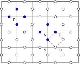
Figure 2: A picture of the cluster charge term $N_{r}=\sum_{r^{\prime}\in r}n_{rr^{\prime}}$ and ring exchange term $\psi_{st}^{\dagger}\psi_{tu}\psi_{uv}^{\dagger}\psi_{vs}(-1)^{N_{s}}$ in (10).

Here, $\psi_{rs}^{\dagger}=e^{i\theta_{rs}}$ denotes the boson creation operator on the bond $\langle rs\rangle$ and $n_{rs}$ is the corresponding boson number operator. (As in the previous section, we will work in the number-phase or quantum rotor representation of the bosons with $[\theta_{rs},n_{rs}]=i$).

The above Hamiltonian is essentially a boson ring exchange model with some frustration. The $u$ term is an on-site repulsion term while $\mu$ is a chemical potential. The $U$ term is a cluster charging term where the clusters - labeled by $r$ - consist of the four bond-centered sites $\langle rr^{\prime}\rangle$ neighboring a site $r$ of the square lattice (see Fig. 2). The operator $N_{r}$ is the total boson number on these four bonds:

$$N_{r}=\sum_{r^{\prime}\in r}n_{rr^{\prime}}$$ (11)

The $K$ term is a ring exchange term involving four bond centered sites adjoining a plaquette $stuv$. This is the usual ring exchange term except for the additional phase $(-1)^{N_{s}}$ which depends on the cluster charge on the upper left hand corner of the plaquette, $s$ (see Fig. 2). This phase can be thought of as some kind of frustration.

Finally, the $t$ term is a boson hopping term between neighboring bond centered sites. Again, this is the usual boson hopping term except for the additional phase $(-1)^{N_{rst}}$. Here, $N_{rst}=b_{rst}+n_{rst}$ where $b_{rst}=0,1$ depending on the specific geometry of $r,s,t$, and $n_{rst}$ is the total boson number of two sites near $r,s,t$ - the location of which also depends on the geometry of $r,s,t$ (see Fig. 3).

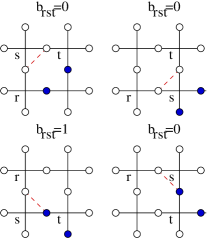
Figure 3: A picture of the boson hopping term $\psi_{rs}^{\dagger}\psi_{st}(-1)^{N_{rst}}$. The operator $N_{rst}=b_{rst}+n_{rst}$ where $b_{rst}=0,1$ and $n_{rst}$ is the total boson number on two sites near $r,s,t$. The value of $b_{rst}$ and the location of the two sites is different for the four possible geometries of $r,s,t$. The sites are denoted above as filled circles.

One way to understand the physics of this model is to consider a related model without the additional factor of $(-1)^{N_{s}}$ in the ring exchange term and $(-1)^{N_{rst}}$ in the hopping term. If we removed these factors, the model would be very similar to the Bose-Hubbard models discussed in LABEL:MS0204,Walight,MS0312,HFB0404. Thus, like in LABEL:MS0204,Walight,MS0312,HFB0404 it could be mapped onto lattice $U(1)$ gauge theory coupled to bosonic charges. In brief, this mapping is given by setting $n_{rs}=\epsilon_{r}E_{rs}$, $\psi_{rs}^{\dagger}=b_{r}^{\dagger}b_{s}^{\dagger}e^{i\epsilon_{r}A_{rs}}$ where $E_{rs},A_{rs}$ are the lattice electric field and vector potential, while $b_{r}^{\dagger}$ denotes the lattice boson creation operator. Under this mapping the $u$ term maps onto an electric energy term $E_{rs}^{2}$, the $K$ term maps onto a magnetic energy term $\cos(A_{st}+A_{tu}+A_{uv}+A_{vs})$ and the $t$ term and $U$ terms map onto hopping terms and mass terms for the bosons $b_{r}$.

The additional factors of $(-1)^{N_{s}},(-1)^{N_{rst}}$ modify this physics in a simple way. First, consider the factor of $(-1)^{N_{s}}$ in the ring exchange term. This factor flips the sign of the ring exchange term if there is a boson $b_{s}$ at site $s$. Since this term corresponds to the magnetic energy term $\cos(A_{st}+A_{tu}+A_{uv}+A_{vs})$ in the lattice gauge theory, this change in sign means that the plaquette $stuv$ prefers to have a flux of $\pi$ instead of $0$. Thus, the effect of the factor of $(-1)^{N_{s}}$ is to energetically bind $\pi$ flux to the bosonic charges $b_{s}$. The lowest energy charge excitation is therefore a composite of a bosonic charge and a $\pi$ flux. Similarly, one can see that the effect of the $(-1)^{N_{rst}}$ in the $t$ term is to make the flux hop together with the charges. Since a bound state of a bosonic charge and a $\pi$ flux is a fermion, the net result is that the low energy effective theory for (10) maps onto a lattice model of fermions coupled to a $U(1)$ gauge field instead of bosons.

In the following, we give a careful derivation of this result. We derive the mapping to fermionic gauge theory from first principles. We then show that the fermions can become gapless and open up a Fermi surface for appropriate parameters - leading to a non-Fermi liquid metallic phase. Specifically, we show that the non-Fermi liquid metallic phase occurs in the regime where $t\ll U$ and $u\ll K,t$ and $|U-\mu/2|<8t$.

We first suppose that $t=u=0$ and then later consider the case of nonzero $t,u$. When $t=u=0$, the Hamiltonian reduces to

$$H=U\sum_{\boldsymbol{r}}(N_{\boldsymbol{r}}-\mu/4U)^{2}-K\sum_{\langle stuv\rangle}(\psi_{st}^{\dagger}\psi_{tu}\psi_{uv}^{\dagger}\psi_{vs}(-1)^{N_{s}}+h.c.)$$

(where we have used the identity $\mu\sum_{\langle rs\rangle}n_{rs}=\mu/2\sum_{r}N_{r}$).

This Hamiltonian is exactly soluble since the operators $\{N_{r}\},\{\psi_{st}^{\dagger}\psi_{tu}\psi_{uv}^{\dagger}\psi_{vs}(-1)^{N_{s}}\}$ all commute. Denoting the simultaneous eigenstate with $N_{r}=n_{r}$, $\psi_{st}^{\dagger}\psi_{tu}\psi_{uv}^{\dagger}\psi_{vs}(-1)^{N_{s}}=e^{i\phi_{stuv}}$ by $|n_{r},\phi_{stuv}\rangle$, it is clear that $|n_{r},\phi_{stuv}\rangle$ is an eigenstate of the Hamiltonian with energy

$$E=U\sum_{r}(n_{r}-\mu/4U)^{2}-2K\sum_{\langle stuv\rangle}\cos(\phi_{stuv})$$ (12)

Assume that $\mu$ is close to, but slightly less than $2U$. In that case the state $|n_{r}=0,\phi_{stuv}=0\rangle$ is the ground state. There are two types of low energy excitations: “flux” excitations where $\phi_{stuv}$ is small but nonzero for some plaquette $\langle stuv\rangle$, and “charge” excitations where $n_{r}=1$ for some site $r$. The flux excitations are gapless while the charge excitations have a small but finite gap $U-\mu/2$. Both types of excitations are exact eigenstates and have no dynamics.

Now consider the case where $t$ is nonzero but much smaller than $U$. The $t$ term will give dynamics to the charge excitations. Indeed, one can see from the definition that when one applies the operator $\psi_{rs}^{\dagger}\psi_{st}(-1)^{N_{rst}}$ to a state $|\{n_{r}\},\{\phi_{stuv}\}\rangle$ it increases $n_{r}$ by $1$ and decreases $n_{t}$ by $1$. On the other hand, it does not change the fluxes $\phi_{stuv}$. We conclude that this operator is an effective hopping term for charges: it gives an amplitude for charges to hop from site $t$ to site $r$. Note that this hopping term only moves charges within the $A$ and $B$ sublattices. Thus, there are actually two species of charges - those on the $A$ sublattice and those on the $B$ sublattice.

While we know that the $t$ term gives an nonzero amplitude for charges to hop, we need to understand the phases of these hopping matrix elements. In particular, we need to understand the phases associated with (a) a charge hopping around a plaquette, and (b) two charges exchanging places. We begin with the problem of a charge hopping around a plaquette. We assume a fixed flux configuration $\phi_{stuv}$ since the fluxes are completely static.

Let us focus on a single plaquette $stuv$. We are interested in states where the plaquette contains a single charge at one of the four sites, $s,t,u,v$. We will label these states by $|s\rangle$, $|t\rangle$, $|u\rangle$, and $|v\rangle$. Let us start with the state $|s\rangle$ where the upper left hand corner $s$ is occupied. The term $T_{1}=\psi_{uv}^{\dagger}\psi_{vs}(-1)^{N_{uvs}}$ gives an amplitude for the charge to hop to the lower right hand corner $u$. The term $T_{2}=\psi_{st}^{\dagger}\psi_{tu}(-1)^{N_{stu}}$ gives an amplitude for the charge to hop back to $s$ (see Fig. 4). The total phase acquired by this process is given by

$$e^{i\phi} = \langle s|T_{2}T_{1}|s\rangle$$ (13)

$$= \langle s|\psi_{st}^{\dagger}\psi_{tu}(-1)^{N_{stu}}\psi_{uv}^{\dagger}\psi_{vs}(-1)^{N_{uvs}}|s\rangle$$

$$= -\langle s|\psi_{st}^{\dagger}\psi_{tu}\psi_{uv}^{\dagger}\psi_{vs}|s\rangle$$

where the last line follows from the fact that $N_{stu}+N_{uvs}=N_{u}+1=1$ for this geometry.

We can rewrite this as:

$$e^{i\phi} = -\langle s|\psi_{st}^{\dagger}\psi_{tu}\psi_{uv}^{\dagger}\psi_{vs}|s\rangle$$ (14)

$$= \langle s|\psi_{st}^{\dagger}\psi_{tu}\psi_{uv}^{\dagger}\psi_{vs}(-1)^{N_{s}}|s\rangle$$

$$= e^{i\phi_{stuv}}$$

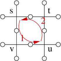
Figure 4: A charge at site $s$ has a nonzero matrix element to hop to site $u$ via the operator $T_{1}=\psi_{uv}^{\dagger}\psi_{vs}(-1)^{N_{uvs}}$. There is also a nonzero matrix element to return to site $s$ via the operator $T_{2}=\psi_{st}^{\dagger}\psi_{tu}(-1)^{N_{stu}}$. The total phase accumulated in this process can be shown to be $e^{i\phi_{stuv}}$.

One can also show that the phase acquired when the charge starts in the lower right hand corner $u$ is $e^{i\phi_{stuv}}$; when the charge starts in the other two corners, one finds that the phase is $e^{-i\phi_{stuv}}$. Thus, the charge excitations couple to the fluxes as if they carry a gauge charge. Since the sign of the coupling is different when the charges are at $s,u$ or $t,v$, we see that the charges on the $A$ and $B$ sublattices carry opposite gauge charges $\pm 1$.

Next we compute the phase acquired when two charges exchange places. To this end, we consider the two hopping processes (A),(B) shown in Fig. 5. The two processes both start with a state where there are charges at sites $r$ and $w$, and end with a state with charges at sites $t$ and $v$.

In process (A), the charge at site $r$ hops to $t$ via the hopping operator $T_{1}=\psi_{st}^{\dagger}\psi_{rs}(-1)^{N_{rst}}$, and then hops from $t$ to $v$ via the hopping operator $T_{2}=\psi_{uv}^{\dagger}\psi_{tu}(-1)^{N_{tuv}}$. The charge at site $w$ then hops to $t$ via the operator $T_{3}=\psi_{tx}^{\dagger}\psi_{wx}(-1)^{N_{wxt}}$. In process (B), the order of the three hops is reversed: the charge at site $w$ hopes to $t$ via the operator $T_{3}$ and then hops from $t$ to $v$ via the operator $T_{2}$. Finally, the charge at site $r$ hops to $t$ via $T_{1}$.

Notice that the difference between the two processes is that in process (A), the charges move from $r\rightarrow v$, and $w\rightarrow t$, while in process (B), the charges move from $w\rightarrow v$, and $r\rightarrow t$. Thus the difference between the two phases accumulated in the two processes should tell us the phase associated with exchanging the particles.

Simple algebra shows that

$$T_{3}T_{2}T_{1}=-T_{1}T_{2}T_{3}$$ (15)

so that there is an extra phase of $\pi$ accumulated in process (A) relative to process (B). We conclude that the charges are fermions. (Indeed, the relation (15) is exactly the “fermionic hopping algebra” from LABEL:LW0316).

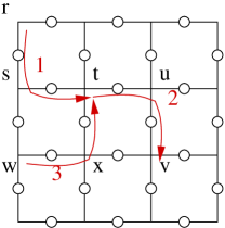
Figure 5: Two processes (A),(B) in which two charges starting at sites $r,w$ can move to sites $t,v$. In process (A), the charge at $r$ hops to $t$ via $T_{1}=\psi_{st}^{\dagger}\psi_{rs}(-1)^{N_{rst}}$ and from $t$ to $v$ via $T_{2}=\psi_{uv}^{\dagger}\psi_{tu}(-1)^{N_{tuv}}$. The charge at $w$ then hops to $t$ via $T_{3}=\psi_{tx}^{\dagger}\psi_{wx}(-1)^{N_{wxt}}$. In process (B), the order of the hops is reversed: the charge at $w$ hops to $t$ via $T_{3}$, and then to $v$ via $T_{2}$. The charge at $r$ then hops to $t$ via $T_{1}$.

To summarize, we have shown that when $u=0$, $t\ll U$, and $\mu$ is close to $2U$ the low energy physics of (10) is described by two species of fermionic quasiparticles carrying opposite gauge charge minimally coupled to a compact $U(1)$ gauge field at zero coupling constant (e.g. no $E^{2}$ term). In fact, the above calculations imply that the low energy physics of (10) can be exactly mapped onto a fermionic lattice gauge theory. (There is one technical issue with this mapping, however. The corresponding lattice gauge theory differs from standard lattice gauge theory in that it contains an additional short distance interaction between fermions which occupy neighboring sites. This interaction applies to the situation where a fermion hops from site $t$ to site $r$ via $\psi_{rs}^{\dagger}\psi_{st}$ in the presence of another fermion at site $s$. As we do not expect this short distance interaction to change the universal long distance physics, we will ignore it here. In any case, if the reader is concerned about this point, we would like to mention that this interaction can be eliminated completely at the cost of using a more complicated model Hamiltonian (10). See LABEL:LWqed for a discussion).

Depending on the values of $\mu,t$ the fermions can be gapped or can open up a Fermi surface. Here, we are interested in the second case - which occurs for $|U-\mu/2|<8t$. In this case, the fermions will form a (non-interacting) Fermi sea - occupying all single particle states up to energy $\mu/2-U$.

Now imagine we turn on a small $u$, $u\ll K,t$. The $u$ term will give dynamics to the flux configurations - formally $u$ corresponds to an $E^{2}$ term for the gauge field. The result is thus a weak coupling compact $U(1)$ gauge field coupled to a Fermi sea of two species of oppositely charged fermions.

One can check that the fermions carry physical boson number (they each carry boson number $1/2$). Thus, as in the previous example, we expect a non-Fermi liquid metallic state with a possible superconducting pairing instability at low temperature. The only difference is that the underlying degrees of freedom here are bosons, not fermions. Thus, we have an example of a non-Fermi liquid Bose metal.

It is worth mentioning that this construction can easily be modified to give an example of a critical $U(1)$ symmetric spin liquid. The first step is to regard the boson model (10) as a quantum rotor model, setting $L^{z}_{rs}=n_{rs}$, $L^{+}_{rs}=\psi^{\dagger}_{rs}$, etc. One can then obtain a spin $S$ spin model by replacing $L^{z},L^{+}$ by $S^{z},S^{+}$. When $S$ is sufficiently large, we expect the spin model to be in the same phase as the rotor model. This phase is a critical spin liquid described by a Fermi sea of spinons coupled to a $U(1)$ gauge field.

IV Conclusion

In this paper, we have described two microscopic models of non-Fermi liquid metals. In one model the underlying degrees of freedom are fermions; in the other model, the basic degrees of freedom are bosons. The low energy physics of both models is described by a Fermi sea of fractionalized quasiparticles coupled to an emergent $U(1)$ gauge field.

We would like to emphasize that these microscopic models are far from unique. For example, similar models can be constructed (out of either fermions or bosons) whose low energy physics is described by a Fermi sea coupled to a $Z_{2}$ gauge field. These models are even better controlled then the ones presented here, since the fermions are completely non-interacting. There are many other possible constructions as well (such as modifications of Kitaev’s exactly soluble honeycomb model Kitaev (2006)). We hope that, collectively, these models can provide a starting point for thinking about the microscopic physics of non-Fermi liquid metallic phases.