Quantum phase transition in space in a ferromagnetic spin-1 Bose-Einstein condensate

Abstract

A quantum phase transition between the symmetric (polar) phase and the phase with broken symmetry can be induced in a ferromagnetic spin-1 Bose-Einstein condensate in space (rather than in time). We consider such a phase transition and show that the transition region in the vicinity of the critical point exhibits scalings that reflect a compromise between the rate at which the transition is imposed (i.e., the gradient of the control parameter) and the scaling of the divergent healing length in the critical region. Our results suggest a method for the direct measurement of the scaling exponent $\nu$.

I Introduction

Studies of phase transitions have traditionally focused on equilibrium scalings of various properties near the critical point of a homogeneous system. The dynamics of phase transitions presents new interdisciplinary challenges. Nonequilibrium phase transitions may play a role in the evolution of the early Universe kibble . Their analogues can be studied in condensed matter systems zurek . The latter observation led to the series of beautiful experiments eksperymenty (see kibble_today for an up-to-date review) and to the development of the theory based on the universality of critical behavior zurek . The recent progress in cold atom experiments allows for the temporal and spatial control of different systems undergoing a quantum phase transition (QPT) lewenstein ; nature_kurn . These experimental developments call for an in-depth understanding of non-equilibrium QPTs.

A QPT is a fundamental change in the ground state of the system as a result of small variations of an external parameter, e.g., a magnetic field sachdev . In contrast to thermodynamic phase transitions, it takes place ideally at temperature of absolute zero.

The problem of how a quantum system undergoes a transition from one quantum phase to another due to time-dependent (temporal) driving has attracted lots of attention lately dorner ; spiny1 ; spiny2 ; ferro_bodzio_prl ; ferro_bodzio_njp ; austen_and_ueda_1_6 ; spins_sen ; spins_fazio . Basic insights into the QPT dynamics can be obtained through the quantum version dorner ; lz_bodzio of the Kibble-Zurek mechanism (KZM) kibble ; zurek . The KZM recognizes that the time evolution of the quantum system is adiabatic far away from the critical point where the gap in the excitation spectrum is large. The system adjusts to all changes imposed on its Hamiltonian. Near the critical point, however, the gap closes precluding the adiabatic evolution and resulting in the non-equilibrium dynamics. This switch of behavior happens when the system reaction time $\hbar/\Delta$ ($\Delta$ is excitation gap) becomes comparable to the time scale on which the critical point is approached, $\varepsilon/|d\varepsilon/dt|$ ($\varepsilon=|q-q_{c}|$, $q$ is the parameter driving the transition, $q_{c}$ is the location of the critical point). This brings us to

$$\frac{\hbar}{\Delta}=\frac{\varepsilon}{|d\varepsilon/dt|}.$$ (1)

To solve (1) we define $\left|\frac{d}{dt}q(t)\right|=\tau_{Q}^{-1}$. The solution of (1) gives us time $\hat{t}$, left to reaching the critical point, when the non-equilibrium dynamics starts

$$\hat{t}=(\hbar/\Delta_{0})^{1/(1+z\nu)}\tau_{Q}^{z\nu/(1+z\nu)}.$$ (2)

Above we have set $\Delta=\Delta_{0}|q_{c}-q|^{z\nu}$ near the critical point ($z$ and $\nu$ are critical exponents).

The quantum KZM proposes that the non-equilibrium evolution in the neighborhood of the critical point is to a first approximation impulse (diabatic): the state of the system does not change there. Suppose that the system evolves towards the critical point from the ground state far away from it. Thus its properties near the critical point are determined by its ground state properties at a distance $\hat{t}/\tau_{Q}$ from the critical point (the adiabatic regime was abandoned there). As have been shown in spin models (e.g., dorner ; spiny1 ) and ferromagnetic spin-1 Bose-Einstein condensates ferro_bodzio_prl ; ferro_bodzio_njp ; austen_and_ueda_1_6 , this simplification allows for a correct analytical computation of the density of excitations resulting from the non-equilibrium quench.

In this paper we study a quantum phase transition induced by spacial rather than temporal driving. It means that the driving parameter, $q$, depends on position and is independent of time. Such a transition was recently studied in the quantum Ising model platini ; xzurek and the mean-field Ginzburg-Landau theory platini . Here we present the theory of the spatial quench in a ferromagnetic spin-1 Bose-Einstein condensate, which is one of the most flexible physical systems for studies of QPTs.

We focus on the ground state. In the simplest approximation, the local homogeneous approximation (LHA), the system is locally characterized by its homogeneous ground state properties perfectly tracking spatial variations of $q$. This approximation is good far enough from the critical point, where the healing length healing is small compared to the imposed scale of spatial driving. Using the time quench analogy, the system evolves perfectly adiabatically in space away from the spatial critical point, ${\bf r}_{c}$, where $q({\bf r}_{c})=q_{c}$.

Around the critical point, however, the healing length diverges and so the LHA breaks down. The system enters “non-equilibrium” regime similarly as during a time quench. The spatial coupling term in the Hamiltonian (a gradient term in mean-field theories, a spin-spin interaction term in spin models) smoothes out the sharp spatial boundary between the phases predicted by the LHA.

Even more interestingly, these similarities are not only qualitative xzurek . The distance from the spatial critical point where the switch between the two regimes takes place, $\hat{x}$, can be determined by looking at the length scales relevant for the spatial quench. We compare the healing length

$$\frac{\xi_{0}}{|q-q_{c}|^{\nu}},$$ (3)

to the length scale on which the spatial critical point is approached: $\varepsilon/|d\varepsilon/dx|$ assuming that $\varepsilon=|q-q_{c}|$ changes in $x$-direction only. This brings us to the spatial analog of (1)

$$\frac{\xi_{0}}{|q-q_{c}|^{\nu}}=\frac{\varepsilon}{|d\varepsilon/dx|}.$$ (4)

To solve (4) we define $\left|\frac{d}{dx}q(x)\right|=\lambda_{Q}^{-1}$ and get

$$\hat{x}=\xi_{0}^{1/(1+\nu)}\lambda_{Q}^{\nu/(1+\nu)}.$$ (5)

The results (2) and (5) are analogous. Indeed, apart from a slight difference in the scaling exponents – due to the absence of $z$ in (5) – $\hat{t}$ maps onto $\hat{x}$ when time scales $\hbar/\Delta_{0}$ and $\tau_{Q}$ are replaced by length scales $\xi_{0}$ and $\lambda_{Q}$, respectively. This shows striking parallels between quenches in time and space. It is also instructive to note that the same general result, Eq. (5), can be obtained in a different way from the scaling theory platini .

II Model

In the following, we will study a QPT in space in a ferromagnetic spin-1 Bose-Einstein condensate. We consider untrapped clouds: atoms in a box. Such a system can be realized in an optical box trap raizen . Assuming that the condensate is placed in the magnetic field $B({\bf r})$ aligned in the $z$ direction, its mean-field energy functional reads leshouches

$${\cal E}[\Psi]=\int d{\bf r}\ \frac{\hbar^{2}}{2M}|\vec{\nabla}\Psi|^{2}+\frac{c_{0}}{2}\langle\Psi|\Psi\rangle^{2}+\frac{c_{1}}{2}\sum_{\alpha}\langle\Psi|F_{\alpha}|\Psi\rangle^{2}\\ -P\langle\Psi|F_{z}|\Psi\rangle+Q\langle\Psi|F_{z}^{2}|\Psi\rangle,$$

where $F_{\alpha=x,y,z}$ is the spin-1 matrix. The strength of spin independent interactions is $c_{0}=4\pi\hbar^{2}(a_{0}+2a_{2})/3M>0$, while the strength of spin dependent interactions reads $c_{1}=4\pi\hbar^{2}(a_{2}-a_{0})/3M<0$. The constant $a_{S}$ is the s-wave scattering length in the total spin $S$ channel ($a_{0}=101.8a_{B}$, $a_{2}=100.4a_{B}$), and $M$ is the atom mass. The prefactors of linear and quadratic Zeeman shifts are given by $P=\mu_{B}B({\bf r})/2$ and $Q=\mu_{B}^{2}B^{2}({\bf r})/4E_{hf}$, respectively. There $E_{hf}$ is the hyperfine splitting energy.

The wave function has three condensate components, $\psi_{m}$, corresponding to $m=0,\pm 1$ projections of spin-1 onto the magnetic field: $\Psi^{T}=(\psi_{1},\psi_{0},\psi_{-1})$. It is normalized as $\int d{\bf r}\Psi^{\dagger}\Psi=N$, where $N$ is the total number of atoms. The condensate magnetization reads

$$f_{\alpha}=\langle\Psi|F_{\alpha}|\Psi\rangle,\ \alpha=x,y,z.$$

It is convenient to define a dimensionless parameter

$$q({\bf r})=Q({\bf r})/n|c_{1}|,$$

where $n\approx N/V$ is the condensate density ($V$ is the system volume). We consider below setups where $n$ fluctuates negligibly in space. The critical point corresponds to $q_{c}=2$.

III Quench in a ferromagnetic spin-1 Bose-Einstein condensate

Similarly as in our work on time-dependent quench ferro_bodzio_prl ; ferro_bodzio_njp , we assume that $\int d{\bf r}f_{z}=0$. Experimentally, such a constraint can be achieved by putting all atoms into an equal mixture of $m=\pm 1$ magnetic sublevels and letting the sample relax to equilibrium leshouches . The spin conservation ensures that the final and initial states will have the same total $f_{z}$ magnetization: $\int d{\bf r}f_{z}=0$. Additionally, we consider $\psi_{\pm 1,0}\geq 0$ in the ground state: a condition that can be always imposed because ${\cal E}[(|\psi_{1}|e^{i\chi_{1}},|\psi_{0}|e^{i\chi_{0}},|\psi_{-1}|e^{i\chi_{-1}})]\geq{\cal E}[(|\psi_{1}|,|\psi_{0}|,|\psi_{-1}|)].$ This sets $f_{y}({\bf r})=0$. Moreover, our numerical simulations indicate that $f_{z}({\bf r})\approx 0$ in the spatial quench considered here. Thus we investigate the $f_{x}({\bf r})$ condensate magnetization only.

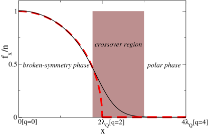
Figure 1: A typical picture of the condensate magnetization in a spatial quench (the black line). The dashed red line shows the magnetization in the local homogeneous approximation, where the healing length is assumed to be negligibly small compared to the length scale of variations imposed on the condensate. The width of the crossover region is proportional to $\hat{x}$ to left and right of the spatial critical point at $x_{c}=2\lambda_{Q}$ [$q(x_{c})=2$ (6)]. This numerical simulation is for $\lambda_{Q}/\lambda_{0}=3/2$ – see Appendix B for numerical details.

For simplicity, we assume that

$$q({\bf r})=\frac{x}{\lambda_{Q}},$$ (6)

and forgetting about the gradient term in (II) – i.e., using our LHA – the ground state phase diagram can be sketched. The part of the condensate exposed to $0\leq q({\bf r})<2$ is in the ground state of the broken-symmetry phase. There $\psi_{\pm 1}^{\rm GS}({\bf r})=\sqrt{n}\sqrt{1/4-q({\bf r})/8}$ and $\psi_{0}^{\rm GS}({\bf r})=\sqrt{n}\sqrt{1/2+q({\bf r})/4}$. The condensate is magnetized: $f_{x}({\bf r})=n\sqrt{1-q({\bf r})^{2}/4}$, while $f_{y,z}({\bf r})=0$. This ground state breaks rotational symmetry on the $(x,y)$ plane present in energy functional (II). Parts of the condensate exposed to $q({\bf r})>2$ are in the polar phase ground state with $\psi_{\pm 1}^{\rm GS}({\bf r})=0$ and $\psi_{0}^{\rm GS}({\bf r})=\sqrt{n}$, which implies $f_{x,y,z}({\bf r})=0$. The dependence of the condensate magnetization on $x$ and $q$ in the LHA is depicted with the red dashed line on Fig. 1. There one condensate accommodates the two phases.

The inclusion of the gradient term in the energy functional (II) prohibits singularities in the first derivative of the wave function. The smooth crossover region replaces the sharp phase boundary predicted by the LHA (Fig. 1). Its size is proportional to $\hat{x}$ (5), as will be carefully discussed below.

In the simplest setup $q({\bf r})$ dependence (6) is achieved by using the static, inhomogeneous, magnetic field to drive the system between the two phases. That would correspond to the following spatial variation of the Zeeman coefficients across a typical ⁸⁷Rb condensate: $\Delta Q\sim n|c_{1}|$ and $\Delta P\sim 10^{4}n|c_{1}|$. The latter result is obtained by using $P=h\times 70\times 10^{4}\times B$ HzG^-1, $Q=h\times 70B^{2}$ HzG^-2 nature_kurn , and $n|c_{1}|/h=9.77$ (evaluated at a peak density of the Berkeley experiment nature_kurn ). As can be found numerically, such an abrupt $P$-variation makes the LHA phase diagram qualitatively incorrect.

To avoid these complications we propose to expose the condensate to the inhomogeneous magnetic field $B$ pointing in the $z$-direction and changing in time faster than the characteristic time scales for the condensate dynamics. When $\langle B(x,t)\rangle_{t}=0$, where $\langle\cdots\rangle_{t}$ denotes time average, the linear Zeeman shift will be wiped out (which we assume from now on), while the quadratic term will be position-dependent only: $Q(x)\sim\langle B(x,t)^{2}\rangle_{t}$. Thus, we are still dealing with a phase transition in space.

To make use of the general predictions worked out in (5), we have to determine the value of the critical exponent $\nu$ and the prefactor $\xi_{0}$ from the generic expression for the healing length (3). We do it by comparing (3) to the expression for a divergent healing length near the critical point (13), which we have derived in Appendix A. We get that $\nu=1/2$ on both sides of the QPT. Introducing a constant

$$\xi_{s}=\sqrt{\hbar^{2}/2Mn|c_{1}|},$$ (7)

we also see from (13) that $\xi_{0}$ equals $\xi_{s}$ in the polar phase and $\xi_{s}/\sqrt{2-2|c_{1}|/c_{0}}$ in the broken-symmetry phase.

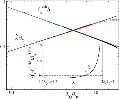
Figure 2: Illustration of various scalings. The black dots: numerics showing the condensate magnetization at the spatial critical point $f_{x}^{\rm crit}=f_{x}(x_{c}=2\lambda_{Q})$. The green line presents the curve $\sim\lambda_{Q}^{-1/3}$. The red crosses and circles show numerics for $\hat{x}$ on the broken-symmetry side of the QPT. The blue line presents power law $\exp(-1.7984)(\lambda_{Q}/\lambda_{0})^{0.3082}$, that was obtained from the fit $\ln\hat{x}/\lambda_{0}=-1.7984\pm 0.0005+(0.3082\pm 0.0004)\ln\lambda_{Q}/\lambda_{0}$, where $\lambda_{0}$ is a unit of length (see Appendix B). The fit was done to data in the range of $\lambda_{Q}/\lambda_{0}\in(1/2,8)$ – red crosses. Red circles show numerical data that was not used for this fit. The determination of $\hat{x}$ is illustrated on the inset showing the data for $\lambda_{Q}/\lambda_{0}=3/2$: $\hat{x}$ is the distance from the critical point where the relative departures of the condensate magnetization from the LHA result, $f_{x}^{\rm LHA}=n\sqrt{1-q(x)^{2}/4}$, start to exceed $10\%$ (other thresholds, $1\%-10\%$, give a similar result). Note logarithmic scale on both axis.

Coming back to (5) we get that the size of the crossover region on either the polar or the broken-symmetry side is

$$\hat{x}=\xi_{0}^{2/3}\lambda_{Q}^{1/3}.$$ (8)

This expression can be verified by looking at experimentally measurable quantity: the ground state magnetization of the condensate nature_kurn .

We start our discussion on the polar side and linearize the wave-function around polar phase ground state: $\psi_{0}=\sqrt{n}(1+\delta\psi_{0})$, $\psi_{\pm 1}=\sqrt{n}\delta\psi_{\pm 1}$, with $\delta\psi_{m}\ll 1$. This leads to $f_{x}=\sqrt{2}n(\delta\psi_{1}+\delta\psi_{-1})+O(\delta\psi_{m}^{2})$. Using position-dependent $q$ from (6) and linearized version of (11) we arrive at

$$\xi_{s}^{2}\vec{\nabla}^{2}f_{x}=\left(\frac{x}{\lambda_{Q}}-2\right)f_{x},$$ (9)

which is solved by

$$f_{x}({\bf r})=f_{x}^{\rm crit}{\rm Ai}\left(\Delta x/(\lambda_{Q}\xi_{s}^{2})^{1/3}\right)/{\rm Ai}(0).$$ (10)

There $f_{x}^{\rm crit}$ is the condensate magnetization at the spatial critical point (it depends on $\lambda_{Q}$ only), $\Delta x=x-2\lambda_{Q}\geq 0$ is the distance from the spatial critical point, and $\rm Ai$ is an Airy function – the only nondivergent solution of (9). This solution rigorously shows that decay of the magnetization, $f_{x}({\bf r})/f_{x}^{\rm crit}$, takes place on a length scale $(\lambda_{Q}\xi_{s}^{2})^{1/3}$ in full agreement with the strikingly simple scaling result (8). Therefore, in the polar phase, the magnetization approaches the LHA value, $f_{x}=0$, at a distance $\hat{x}$ from the critical point.

On the broken-symmetry side of the QPT, we refer to numerics (Appendix B) to verify accuracy of (8). In the two extreme limits, very large and very small $\lambda_{Q}$ the theory does not work well. Indeed, using (6) we see that the spatial extent of the broken-symmetry phase is $2\lambda_{Q}$ (Fig. 1). Thus, we expect that $\hat{x}\ll 2\lambda_{Q}$, i.e., $\lambda_{Q}\gg\xi_{0}/2^{3/2}$, to see well the crossover region on the broken-symmetry side. In the other limit, large $\lambda_{Q}$, we have to take into account that the system size in numerical simulations is finite, say $l$. There we need to have $\lambda_{Q}\ll l/2$ so that there will be a spatial point in our system where $q(x)=2$, and the finite size corrections coming from proximity of the system boundary to the spatial critical point will be negligible. These two estimates tell us that $\lambda_{Q}$ in our system shall be much larger than $0.1\lambda_{0}$ and much smaller than $39\lambda_{0}$ (see Appendix B for numerical value of $l$, $\xi_{0}\approx\xi_{s}/\sqrt{2}$ and the unit of length $\lambda_{0}$ relevant for our simulations). Increasing (decreasing) the lower (upper) limit on $\lambda_{Q}$ by a factor of five we fit a power law to $\lambda_{Q}/\lambda_{0}\in(1/2,8)$. We get from a fit that $\ln\hat{x}/\lambda_{0}=-1.7984\pm 0.0005+(0.3082\pm 0.0004)\ln\lambda_{Q}/\lambda_{0}$ – see Fig. 2. The numerical data for $\hat{x}$ clearly departs from the fitted line for $\lambda_{Q}/\lambda_{0}\gtrsim 10$. Departures for $\lambda_{Q}/\lambda_{0}\lesssim 1/2$ are much less pronounced. Therefore, we get approximately that $\hat{x}\sim\lambda_{Q}^{0.31}$, which is in good qualitative agreement with the predicted scaling, i.e., $\lambda_{Q}^{1/3}$. We expect that better agreement can be obtained for large systems where we can explore larger $\lambda_{Q}$’s for which crossover region is closer to the critical point ($\hat{x}/\lambda_{Q}\sim\lambda_{Q}^{-1/3}$). More precisely, by taking the limit of $N,l,\lambda_{Q}\to\infty$ at $\xi_{0}={\rm const}$ (i.e., $N/l={\rm const}$) we expect that the scaling (8) will be fully recovered from numerical simulations.

Now let’s focus on the magnetization at the critical point. From (10) we know that it scales in the same way as the condensate magnetization at the border of the crossover region in the polar phase ($x_{+}=2\lambda_{Q}+\hat{x}$):

$$f_{x}(x_{+})/n=f_{x}^{\rm crit}{\rm Ai}(1)/{\rm Ai(0)}\sim f_{x}^{\rm crit}.$$

Assuming that similar scaling relation will also hold between $f_{x}^{\rm crit}$ and $f_{x}$ at $x_{-}=2\lambda_{Q}-\hat{x}$, i.e., at the broken-symmetry phase border of the crossover region where

$$f_{x}(x_{-})/n\approx\sqrt{1-q(x_{-})^{2}/4}\approx\sqrt{\hat{x}/\lambda_{Q}}\sim\lambda_{Q}^{-1/3},$$

we get that $f_{x}^{\rm crit}\sim\lambda_{Q}^{-1/3}$. As depicted in Fig. 2, we have indeed a robust $f_{x}^{\rm crit}\sim\lambda_{Q}^{-1/3}$ scaling for $\lambda_{Q}/\lambda_{0}$ in the large range of $10^{-1}$ to $10$. It is quite remarkable that the above intuitive prediction of the $f_{x}^{\rm crit}$ scaling matches numerics so well. It suggests that magnetization at the spatial critical point might be a robust observable for studies of spatial quenches. Similar observation was made for condensate magnetization at the critical point during a temporal quench from the broken-symmetry to the polar phase ferro_bodzio_njp .

All these results are in qualitative agreement with our expectations: in the limit of large $\lambda_{Q}$ – very slow spatial driving – the condensate ground state approaches the LHA. Indeed, both the size of the crossover region in the $q$-parameter space, $\hat{x}/\lambda_{Q}$, and the condensate magnetization at the critical point, $f_{x}^{\rm crit}$, go to zero as $\lambda_{Q}$ increases.

The measurements of the dependence of the size of crossover region on $\lambda_{Q}$ should allow for the first experimental determination of the scaling exponent $\nu$ in a ferromagnetic spin-1 Bose-Einstein condensate. Thus, our considerations lead to the new way of investigating the critical region of phase transitions. Another scheme that can be used to determine the exponent $\nu$ was explored experimentally by Esslinger’s group in the context of the classical phase transition from a normal gas to a Bose-Einstein condensate esslinger . The setup involved in this experiment is quite complicated as it requires presence of a high finesse optical cavity for detection purposes. We expect that the approach proposed by us should be easier to implement in the context of quantum phase transitions. Moreover, according to (5) our scheme shall be also ready for experimental exploration in the whole zoo of other physical systems undergoing a QPT. Finally, we would like to stress that applicability of Eq. (5) is not limited to mean-field theories: any experimental departures from the $\lambda_{Q}^{1/3}$ scaling (apart from finite size corrections) should indicate that mean-field value of the critical exponent $\nu$ does not describe the condensate properly. In such a case the correct value of the $\nu$ exponent should be easily extracted from experimental data with the help of Eq. (5).

IV Summary

We have explored physics of the QPT in space in a ferromagnetic spin-1 Bose-Einstein condensate nature_kurn : the most flexible system for studies of QPTs in space and time. Our scaling results explain how singularities of the critical point affect the ground state magnetization of the condensate. They also suggest a new way for the measurement of the critical exponent $\nu$. These findings are generally applicable to all systems undergoing a second order QPT. The quest for the full understanding of a spatial quench opens up a prospect of interdisciplinary studies similarly as time quenches have done to date kibble_today .

V Acknowledgments

We acknowledge the support of the U.S. Department of Energy through the LANL/LDRD Program.

Appendix A Healing length of a ferromagnetic spin-1 condensate

The key ingredient of our theory is the divergent healing length (3). Below we derive it from mean-field equations

$$-\frac{\hbar^{2}}{2M}\vec{\nabla}^{2}\psi_{\pm 1}+c_{0}(|\psi_{0}|^{2}+|\psi_{1}|^{2}+|\psi_{-1}|^{2})\psi_{\pm 1}+c_{1}(|\psi_{0}|^{2}+|\psi_{\pm 1}|^{2}-|\psi_{\mp 1}|^{2})\psi_{\pm 1}+c_{1}\psi_{0}^{2}\psi_{\mp 1}^{*}+Q\psi_{\pm 1}=\mu\psi_{\pm 1},$$

$$-\frac{\hbar^{2}}{2M}\vec{\nabla}^{2}\psi_{0}+c_{0}(|\psi_{0}|^{2}+|\psi_{1}|^{2}+|\psi_{-1}|^{2})\psi_{0}+c_{1}(|\psi_{1}|^{2}+|\psi_{-1}|^{2})\psi_{0}+2c_{1}\psi_{0}^{*}\psi_{1}\psi_{-1}=\mu\psi_{0},$$ (11)

that come from minimization of ${\cal E}-\mu\int d{{\bf r}}\sum_{m}|\psi_{m}|^{2}$ without the linear Zeeman term (II) – see Sec. III for the explanation of why we remove it from our considerations.

The healing length is a typical length scale over which a local perturbation of the wave-function gets forgotten (here we will have three characteristic length scales, but we will identify the leading one relevant for a long distance healing process). To find it, we assume the constant parameter $q=Q/n|c_{1}|$ across the condensate, and linearize mean-field equations (11). We write the wave-function as $\psi_{m}=\psi_{m}^{\rm GS}+\sqrt{n}\delta\psi_{m}$ with $m=0,\pm 1$ and $\psi_{m}^{\rm GS}$ being the ground state solution. In the broken-symmetry phase we have $\psi_{\pm 1}^{\rm GS}({\bf r})=\sqrt{n}\sqrt{1/4-q({\bf r})/8}$ and $\psi_{0}^{\rm GS}({\bf r})=\sqrt{n}\sqrt{1/2+q({\bf r})/4}$, while in the polar phase, $\psi_{\pm 1}^{\rm GS}({\bf r})=0$ and $\psi_{0}^{\rm GS}({\bf r})=\sqrt{n}$. We use here the freedom to work with $\psi_{0,\pm 1}\geq 0$, which is explained in Sec. III.

Linearized equations take the form

$$\xi_{s}^{2}\vec{\nabla}^{2}\delta\psi_{m}=\sum_{k}S_{mk}\delta\psi_{k},$$ (12)

where $\xi_{s}=\sqrt{\hbar^{2}/2Mn|c_{1}|}$ and $S$ stands for

$$\frac{c_{0}}{4|c_{1}|}\left(\begin{array}[]{ccc}2-qu_{-}&(4+2q)u_{-}&2-qu_{+}\\ (2-q)u_{-}&4+2q&(2-q)u_{-}\\ 2-qu_{+}&(4+2q)u_{-}&2-qu_{-}\end{array}\right),\ u_{\pm}=1\pm 2|c_{1}|/c_{0}$$

in the broken-symmetry phase, and for

$$\left(\begin{array}[]{ccc}q-1&0&-1\\ 0&2c_{0}/|c_{1}|&0\\ -1&0&q-1\end{array}\right)$$

in the polar phase. The factor $u_{\pm}$ above is very close to unity as $|c_{1}|/c_{0}\approx 1/216.1\ll 1$ for ⁸⁷Rb atoms considered here.

To proceed we diagonalize matrix $S$ by the transformation $S=CDC^{-1}$, where $D={\rm diag}(\Gamma_{1},\Gamma_{2},\Gamma_{3})$ is a diagonal matrix made of eigenvalues of matrix $S$. In the polar phase we find

$$\Gamma_{m}=q-2,q,2c_{0}/|c_{1}|,$$

while in the broken-symmetry phase we get

$$\Gamma_{m}=c_{0}/|c_{1}|\mp\sqrt{(c_{0}/c_{1})^{2}-(4-q^{2})(c_{0}/|c_{1}|-1)},q.$$

After defining $\delta\tilde{\psi}_{m}=\sum_{n}C^{-1}_{mn}\delta\psi_{n}$ and some elementary algebra we get

$$\frac{\xi_{s}^{2}}{\Gamma_{m}}\vec{\nabla}^{2}\delta\tilde{\psi}_{m}=\delta\tilde{\psi}_{m}\Rightarrow\delta\tilde{\psi}_{m}=f\left(\frac{{\bf r}}{\xi_{s}/\sqrt{\Gamma_{m}}}\right),$$

where the form of the function $f$ depends on system dimensionality (1D, 2D, or 3D), while ${\bf r}$ is “attached” to the point in space where the perturbation is imposed on the wave-function. This solution implies that the eigenvalue vanishing at the critical point, $\Gamma_{\rm min}$, provides the leading contribution to the long-distance healing process near the critical point ($q\approx 2$). Indeed, a simple calculation shows that the wave function will forget about the perturbation imposed on it ($\delta\psi_{m},\delta\tilde{\psi}_{m}\approx 0$) at a distance scaling as $\xi_{s}/\sqrt{\Gamma_{\rm min}}$. Thus, the divergent healing length equals $\xi_{s}/\sqrt{\Gamma_{\rm min}}$. Around the critical point we find it to be

$$\xi^{\rm broken}=\frac{\xi_{s}}{\sqrt{2-2|c_{1}|/c_{0}}|q-2|^{1/2}},\ \ \xi^{\rm polar}=\frac{\xi_{s}}{|q-2|^{1/2}}$$ (13)

on the broken-symmetry ($q<2$) and polar ($q>2$) sides of the QPT, respectively. The expansion around $q=2$ was applied to obtain $\xi^{\rm broken}$, i.e., we have approximated the eigenvalue $c_{0}/|c_{1}|-\sqrt{(c_{0}/c_{1})^{2}-(4-q^{2})(c_{0}/|c_{1}|-1)}$ by $(2-2|c_{1}|/c_{0})(2-q)$ near the critical point. These expressions fix the value of the mean-field critical exponent $\nu$ for our model: $\nu=1/2$ (compare (13) to (3)). We conclude by showing another simplification of the full expression for the divergent healing length on the broken symmetry side. Taking the limit of $|c_{1}|/c_{0}\to 0$, well justified for ⁸⁷Rb, we get

$$\xi^{\rm broken}=\frac{\xi_{s}\sqrt{2}}{\sqrt{4-q^{2}}},$$

without restricting ourselves to $q\approx 2$.

Appendix B Details of numerical simulations

Our analytical predictions are valid in any dimensional system, but we test them numerically in a 1D model. Our numerics is based on conjugate gradient minimization of the 1D energy functional

$$\int d\tilde{x}\ \frac{1}{2}\frac{d\tilde{\Psi}^{T}}{d\tilde{x}}\frac{d\tilde{\Psi}}{d\tilde{x}}+\frac{\tilde{c}_{0}}{2}\langle\tilde{\Psi}|\tilde{\Psi}\rangle^{2}+\frac{\tilde{c}_{1}}{2}\sum_{\alpha=x,y,z}\langle\tilde{\Psi}|F_{\alpha}|\tilde{\Psi}\rangle^{2}\\ +q\tilde{n}|\tilde{c}_{1}|\langle\tilde{\Psi}|F_{z}^{2}|\tilde{\Psi}\rangle,$$

obtained through dimensional reduction of the full 3D energy functional (II) without the linear Zeeman term – see Sec. III for the explanation of why we remove it from our considerations. Moreover, all the components of the above energy functional are dimensionless, and chosen to match qualitatively the experiment of the Berkeley group nature_kurn . Derivation of (B) is explained in detail in ferro_bodzio_prl : please account for different normalization of the wave-function between this paper and ferro_bodzio_prl .

In short, we have $N$, number of atoms, equal to $2\times 10^{6}$, $N\tilde{c}_{1}=-629$, and $\tilde{c}_{0}=216.1|\tilde{c}_{1}|$. The unit of length used through the paper, $\lambda_{0}$, equals $5.1\mu m$. The system (box) size is $\tilde{l}=l/\lambda_{0}=78$, i.e., about $0.4mm$ ($\tilde{l}\times\lambda_{0}$). The coordinate $\tilde{x}$ runs from $0$ to $\tilde{l}$. The density, $\tilde{n}$, equals $N/\tilde{l}$, while $\int d\tilde{x}\tilde{\Psi}^{T}\tilde{\Psi}=N$. The “prefactor” of the healing length, $\xi_{s}$ (7), in these dimensionless quantities is $\sqrt{\tilde{l}/2N|\tilde{c}_{1}|}\approx 1/4$, i.e., about $1.3\mu m$ ($\lambda_{0}/4$).

References

- (1) T.W.B. Kibble, J. Phys. A 9, 1387 (1976); Phys. Rep. 67, 183 (1980).
- (2) W.H. Zurek, Nature (London) 317, 505 (1985); Acta Phys. Pol. B 24, 1301 (1993); Phys. Rep. 276, 177 (1996).
- (3) I. Chuang et al., Science 251, 1336 (1991); M.J. Bowick et al., ibid. 263, 943 (1994); C. Bauerle et al., Nature (London) 382, 332 (1996); V.M.H. Ruutu et al., ibid. 382, 334 (1996); A. Maniv, E. Polturak, and G. Koren, Phys. Rev. Lett. 91, 197001 (2003); S. Ducci et al., ibid. 83, 5210 (1999); R. Monaco et al., ibid. 96, 180604 (2006); D.R. Scherer, C.N. Weiler, T.W. Neely, and B. P. Anderson, ibid. 98, 110402 (2007). S. Casado et al., Eur. Phys. J. Special Topics 146, 87 (2007).
- (4) T.W.B. Kibble, Physics Today 60, 47 (2007).
- (5) M. Lewenstein, A. Sanpera, V. Ahufinger, B. Damski, A. Sen, and U. Sen, Adv. Phys. 56, 243 (2007).
- (6) L.E. Sadler, J.M. Higbie, S.R. Leslie, M. Vengalattore, and D.M. Stamper-Kurn, Nature (London) 443, 312 (2006).
- (7) S. Sachdev, Quantum Phase Transitions (Cambridge University Press, Cambridge UK, 2001).
- (8) W.H. Zurek, U. Dorner, and P. Zoller, Phys. Rev. Lett. 95, 105701 (2005).
- (9) J. Dziarmaga, Phys. Rev. Lett. 95, 245701 (2005).
- (10) R.W. Cherng and L.S. Levitov, Phys. Rev. A 73, 043614 (2006); L. Cincio, J. Dziarmaga, M.M. Rams, and W.H. Zurek, ibid. 75, 052321 (2007); A. Fubini, G. Falci, and A. Osterloh, New J. Phys. 9, 134 (2007).
- (11) B. Damski and W.H. Zurek, Phys. Rev. Lett. 99, 130402 (2007).
- (12) B. Damski and W.H. Zurek, New J. Phys. 10, 045023 (2008).
- (13) A. Lamacraft, Phys. Rev. Lett. 98, 160404 (2007); H. Saito, Y. Kawaguchi, and M. Ueda, Phys. Rev. A 76, 043613 (2007).
- (14) D. Sen, K. Sengupta, and S. Mondal, Phys. Rev. Lett. 101, 016806 (2008); K. Sengupta, D. Sen, and S. Mondal, ibid. 100, 077204 (2008); U. Divakaran, A. Dutta, and D. Sen, Phys. Rev. B 78, 144301 (2008); V. Mukherjee, U. Divakaran, A. Dutta, and D. Sen, ibid. 76, 174303 (2007).
- (15) D. Patanè, A. Silva, L. Amico, R. Fazio, and G.E. Santoro, Phys. Rev. Lett. 101, 175701 (2008); T. Caneva, R. Fazio, and G.E. Santoro, Phys. Rev B 76, 144427 (2007); T. Caneva, R. Fazio, and G.E. Santoro ibid. 78, 104426 (2008); F. Pellegrini, S. Montangero, G.E. Santoro, and R. Fazio, ibid. 77, 140404 (2008).
- (16) B. Damski, Phys. Rev. Lett. 95, 035701 (2005); B. Damski and W.H. Zurek, Phys. Rev. A 73, 063405 (2006).
- (17) T. Platini, D. Karevski, and L. Turban, J. Phys. A 40, 1467 (2007).
- (18) W.H. Zurek and U. Dorner, Phil. Trans. R. Soc. A 366, 2953 (2008).
- (19) The healing length is the typical distance over which a system can adjust to a local perturbation imposed on it.
- (20) T.P. Meyrath, F. Schreck, J.L. Hanssen, C.-S. Chuu and M.G. Raizen, Phys. Rev. A 71, 041604(R) (2005).
- (21) D.M. Stamper-Kurn and W. Ketterle, Coherent atomic matter waves, Proc. Les Houches Summer School, Course LXXII, 1999 ed R. Kaiser, C. Westbrook, and F. David (Springer, New York, 2001).
- (22) T. Donner, S. Ritter, T. Bourdel, A. Öttl, M. Köhl, and T. Esslinger, Science 315, 1556 (2007).