Optimal Time to Sell a Stock in Black-Scholes Model: Comment on “Thou shall buy and hold”, by A. Shiryaev, Z. Xu and X.Y. Zhou

Abstract

We reconsider the problem of optimal time to sell a stock studied by Shiryaev, Xu and Zhou SXZ using path integral methods. This method allows us to confirm the results obtained by these authors and extend them to a parameter region inaccessible to the method used in SXZ . We also obtain the full distribution of the time $t_{m}$ at which the maximum of the price is reached for arbitrary values of the drift.

I Introduction

In the preceeding paper, A. Shiryaev, Z. Xu and X.Y. Zhou SXZ ask about the optimal time to sell a stock over a certain time interval $[0,T]$, knowing that the price is a geometrical Brownian motion with a certain average return over the risk-free rate $a-r$ and a certain volatility $\sigma$. The answer to this question depends on the value of the adimensional parameter $\alpha=(a-r)/\sigma^{2}$. The method used by the authors allow them to prove that whenever $\alpha>1/2$ the optimal selling time $\tau^{*}$ is always at the end of the interval, $\tau^{*}=T$, whereas $\tau^{*}=0$ in the case $\alpha<0$. In financial words, “good” stocks with a sufficiently large average return should be sold as late as possible, whereas one should immediately get rid of “bad stocks”. These results are clearly very interesting; however one feels unsatisfied by the fact that the authors’ method do not allow them to treat the case $0<\alpha\leq 1/2$. They discuss this point in the conclusion, mentioning (a) a working paper SXZ2 based on an alternative method showing that one should in fact sell immediately as soon as $\alpha<1/2$ and (b) that the case $\alpha<1/2$ is not interesting financially because “most stocks realize $\alpha>1/2$ by a large margin”.

The aim of this short note is to reconsider the problem using path integral methods which are well known in physics but perhaps less well known in financial mathematics. This method allows one to treat all values of $\alpha$ on the same footing. We confirm the results of SXZ and extend them to the $0<\alpha\leq 1/2$ interval. In fact, we show that there is an exact symmetry in the problem that relates the problem with $\alpha>1/2$ to the problem with $\alpha<1/2$. Our method furthermore allows us to garner additional results, such as the distribution of the time $t_{m}$ at which the maximum of the price is reached. We find that this distribution has inverse square root singularities both at $t_{m}=0$ and $t_{m}=T$ for all values of $\alpha$; however, the amplitude of the divergence at $t_{m}=0$ is stronger when $\alpha<1/2$ and weaker when $\alpha>1/2$. This gives a more precise picture to the results of Shiryaev, Xu and Zhou. For $\alpha=1/2$, the problem is degenerate and the two peaks have exactly the same amplitude (in fact, the distribution is symmetric under $t_{m}\to T-t_{m}$).

Finally, we do not agree with the statement that $\alpha<1/2$ is not interesting financially. The numbers provided in SXZ are based on the S&P500 index returns, and are therefore much too optimistic: first, there is an obvious selection bias since badly performing stocks leave the index; second, the volatility of the index is two to three times smaller than the volatility of individual stocks, thanks to the diversification effect. An annualized volatility above $40\%$ is in fact not uncommon, in particular for small to medium caps – whereas the S&P500 only includes large caps. Fig. 1 shows the time series of the (implied) S&P500 index volatility and the average stock volatility, in the period 2000-2007. With an average annual return of $10\%$, an interest rate of $5\%$ and a volatility of $40\%$ annual, the parameter $\alpha$ is found to be $0.3125<1/2$.

We hope that this short note will shed a useful light on the work of A. Shiryaev, Z. Xu and X.Y. Zhou, and that it will convince the reader that path integral methods are extremely powerful to solve a variety of random walk problems. We refer the reader to a short review paper by one of us BF on this topic, see also MRKY .

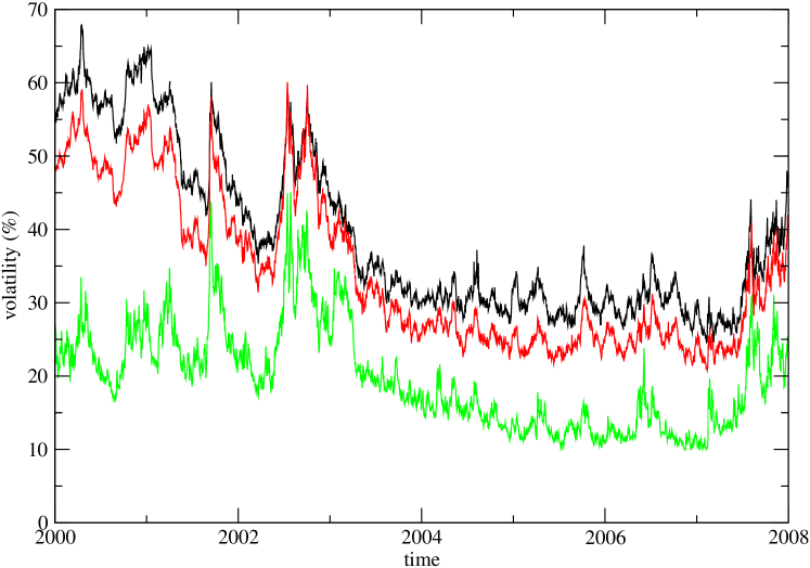
Figure 1: Time series of the (implied) S&P500 index volatility (the VIX, bottom green curve) and the average implied stock volatility for SPX stocks (middle red curve) and mid-cap stocks (upper black curve), in the period 2000-2007. It is clear that stock volatilities are on average two to three times larger than the volatility of the index, and that values of $\sigma$ above $40\%$ are not uncommon.

II The Set-Up

In this section we give the set-up of the problem using physicists notations. We assume, as in SXZ , that the price $P_{t}$ of a stock follows a geometric Brownian motion:

$$P_{t}=\exp\left[\mu t+\sigma\,B_{t}\right],$$ (1)

where $\mu$ is Ito corrected drift and $B_{t}$ the standard Brownian motion. We will use below the notation $x(t)=\mu t+\sigma B_{t}$ for the drifted Brownian motion, with by convention $x(0)=0$. In Ref. SXZ , the authors introduce the notation $\alpha=\mu/\sigma^{2}+1/2$. A ‘good’ stock in the financial language corresponds to a positive drift $\mu>0$ (i.e., $\alpha>1/2$) and a ‘bad’ stock corresponds to a negative drift $\mu<0$ ($\alpha<1/2$). In terms of the real return $a$ of the stock, the condition $\mu>0$ translates into $a-r>\sigma^{2}/2$, where $a-r$ is the excess return over the risk-free rate $r$. Note that the process that we talk about is the real world process and not the risk-neutral one, which has no meaning for the question raised in Ref. SXZ .

Let us consider the evolution of the stock price over a fixed time interval $0\leq t\leq T$. It is intuitively obvious that the maximum of a drifted Brownian motion and hence that of the stock price $P_{t}$ is most likely to occur at $t=T$ (for $\mu>0$) and $t=0$ (for $\mu<0$). Thus, it obviously makes sense to sell a ‘good’ stock $(\mu>0)$ at the end of the interval $t=T$, whereas a ‘bad’ stock $(\mu<0)$ at the begining of the interval $t=0$. This intuitive results are put on a more rigorous mathematical footing in the rest of this note by (i) calculating exactly, using path integral methods, the maximal relative error as defined in Ref. SXZ , but for all values of $\mu$ and (ii) also by computing the full probability density of the time $t_{m}$ at which the maximum of the price occurs for all $\mu$.

Let $M_{T}$ denote the maximum price of the stock over the interval $[0,T]$, i.e.,

$$M_{T}=\max_{\begin{subarray}{c}0\leq t\leq T\end{subarray}}P_{t}.$$ (2)

Evidently, the optimal time to sell the stock is the one where the difference between the price of the stock and its maximal value $M_{T}$ is minimal. A convenient way to estimate this optimal time is to consider the relative error at a fixed time $\tau$ where $0\leq\tau\leq T$

$$r_{\mu}(\tau,T)={\rm E}\left(\frac{M_{T}-P_{\tau}}{M_{T}}\right)=1-{\rm E}\left(\frac{P_{\tau}}{M_{T}}\right)$$ (3)

where ${\rm E}$ denotes the expectation value over all realizations of the Brownian motion. Minimizing $r_{\mu}(\tau,T)$ over $0\leq\tau\leq T$ gives the optimal time $\tau^{*}$. In other words, $\tau^{*}$ is the time at which the ratio

$$S_{\mu}(\tau,T)=1-r_{\mu}(\tau,T)={\rm E}\left(\frac{P_{\tau}}{M_{T}}\right)$$ (4)

is maximal. The goal is to estimate $S_{\mu}(\tau,T)$ and then maximize it with respect to $0\leq\tau\leq T$. Using the trivial identity

$$M_{T}=\max_{\begin{subarray}{c}0\leq\tau\leq T\end{subarray}}P_{\tau}=\max_{\begin{subarray}{c}0\leq\tau\leq T\end{subarray}}\left[\exp\left(x(\tau)\right)\right]=\exp\left[\max_{\begin{subarray}{c}0\leq\tau\leq T\end{subarray}}x(\tau)\right]$$ (5)

one can rewrite $S_{\mu}(\tau,T)$ in Eq. (4) as

$$S_{\mu}(\tau,T)={\rm E}\left[\exp\left(-\{\tilde{M}_{T}-x(\tau)\}\right)\right]$$ (6)

where

$$\tilde{M}_{T}=\max_{\begin{subarray}{c}0\leq t\leq T\end{subarray}}x(t)=\ln[M_{T}]$$ (7)

is the maximum of the drifted Brownian motion $x(t)$ over $0\leq t\leq T$. Note that throughout this paper, we will use $t$ as the running time and $\tau$ as a fixed time.

Let us consider the random variable $y(\tau)=\tilde{M}_{T}-x(\tau)$ at a fixed time $\tau$ and let $P_{\mu}(y,\tau)$ denote its probability density function (pdf). Once we know $P_{\mu}(y,\tau)$, then from Eq. (6), we can evaluate

$$S_{\mu}(\tau,T)=\int_{0}^{\infty}dy\,e^{-y}\,P_{\mu}(y,\tau).$$ (8)

To evaluate the pdf $P_{\mu}(y,\tau)$, we need the joint pdf of $\tilde{M}_{T}$ and $x(\tau)$ at fixed $\tau$.

III Joint distribution of $\tilde{M}_{T}$ and $x(\tau)$

It is convenient to compute first the cumulative probability

$$F_{\mu}(x,m,\tau)={\rm Prob}[x(\tau)=x\,\,{\rm and}\,\,\tilde{M}_{T}\leq m]$$ (9)

where the walk starts at the origin $x(0)=0$ and $\tilde{M}_{T}$ is the global maximum of the walk in $[0,T]$. This cumulative probability can be computed using a path-integral approach as detailed below.

Clearly $F_{\mu}(x,m,\tau)$ is the probability that a drifted Brownian motion $x(t)$ in $0\leq t\leq T$, starting from $x(0)=0$, reaches $x(\tau)=x$ at a fixed time $t=\tau$ and in addition, stays below the level $m$ for all $0\leq t\leq T$. The last condition comes from the fact that if the global maximum $\tilde{M}_{T}\leq m$, the path necessarily stays below the level $m$ for all $0\leq t\leq T$. An example of such a path is seen in Fig. 2.

Figure 2: A realization of the drifted Brownian motion $x(t)$ in $t\in[0,T]$, starting at $x(0)=0$, reaching $x(\tau)=x$ at $t=\tau$ and staying below the level $m$ for all $0\leq t\leq T$.

To compute $F_{\mu}(x,m,\tau)$, it is convenient to consider the shifted process $y(t)=m-x(t)$ so that the process $y(t)$ evolves, as

$$dy=-dx=-\mu dt-\sigma dB_{t}.$$ (10)

Thus the shifted process $y(t)$ represents a Brownian motion with a drift $-\mu$, opposite to that of $x(t)$. In terms of the process $y(t)$, $F_{\mu}(x,m,\tau)$ is just the probability that the process $y(t)$, starting at $y(0)=m$, reaches the point $y(\tau)=m-x$ at $t=\tau$ and stays positive in the whole interval $0\leq t\leq T$. An example of such an event is shown in Fig. 3

Figure 3: A realization of the shifted Brownian motion $y(t)$ with drift $-\mu$ in $t\in[0,T]$, starting at $y(0)=m$, reaching $y(\tau)=m-x$ at $t=\tau$ and staying positive for all $0\leq t\leq T$.

For the process $y(t)$ in Eq. (10), let us first define the propagator $G_{-\mu}^{+}(y,y_{0},t)$ that denotes the probability that the process starting at $y_{0}$ at $t=0$, reaches $y$ at time $t$, but staying positive in between, i.e., in $[0,t]$. One can then easily express $F_{\mu}(x,m,\tau)$ in terms of this propagator as (see Fig. 3)

$$F_{\mu}(x,m,\tau)=G_{-\mu}^{+}(m-x,m,\tau)\,\int_{0}^{\infty}G_{\mu}^{+}(y^{\prime},m-x,T-\tau)\,dy^{\prime}.$$ (11)

In writing Eq. (11), we have split the interval $[0,T]$ into two parts: $[0,\tau]$ and $[\tau,T]$. In the first interval (see Fig. 3), the process propagates from the initial position $y(0)=m$ to $y(\tau)=m-x$ in time $\tau$ (staying positive in between), hence explaining the first factor $G_{-\mu}^{+}(m-x,m,\tau)$ in Eq. (11). In the second interval, the process starting at the new ‘initial’ position $m-x$, propagates to a final position $y^{\prime}$ in time $T-\tau$, staying positive in between. Also, the final position $y^{\prime}$ can be any positive number and one has to integrate over it. This explains the second factor in Eq. (11). Of course, in writing the path decomposition in Eq. (11) we have used the renewal property of a Brownian motion (valid due to its Markovian nature) which implies that the two intervals (left of $\tau$ and right of $\tau$) are statistically independent.

Evaluation of the propagator $G_{-\mu}^{+}(y,y_{0},\tau)$: Using a physicist interpretation of Eq. (10), we note that the Langevin noise $\eta(t)=dB_{t}/dt$ is a Gaussian white noise with the associated measure, ${\rm Prob}\left[\{\eta(t)\},0\leq t\leq\tau\right]\propto\exp\left[-\frac{1}{2}\int_{0}^{\tau}\eta^{2}(t)dt\right]$. Substituting, $\eta(t)=({\dot{y}}+\mu)/\sigma$ from Eq. (10), one can express the propagator as a path integral

$$G_{-\mu}^{+}(y,y_{0},\tau)=\int_{y(0)=y_{0}}^{y(\tau)=y}{\cal D}y(t)\exp\left[-\frac{1}{2\sigma^{2}}\int_{0}^{\tau}dt\left({\dot{y}}+\mu\right)^{2}\right]\,\left[\prod_{t=0}^{\tau}\theta(y(t))\right]$$ (12)

where $\left[\prod_{t=0}^{\tau}\theta(y(t))\right]$ is an indicator function that enforces the path to stay positive in the interval $t\in[0,\tau]$. The rhs of Eq. (12) can be rearranged (by expanding the square $({\dot{y}}+\mu)^{2}$ and performing the time integral) as

$$G_{-\mu}^{+}(y,y_{0},\tau)=\exp\left[-\frac{\mu^{2}\tau}{2\sigma^{2}}-\frac{\mu}{\sigma^{2}}(y-y_{0})\right]\,G_{0}^{+}(y,y_{0},\tau)$$ (13)

where $G_{0}^{+}(y,y_{0},\tau)$ is the propagator associated with the driftless $(\mu=0)$ Brownian motion

$$G_{0}^{+}(y,y_{0},\tau)=\int_{y(0)=y_{0}}^{y(\tau)=y}{\cal D}y(t)\exp\left[-\frac{1}{2\sigma^{2}}\int_{0}^{\tau}dt\,{\dot{y}}^{2}\right]\,\left[\prod_{t=0}^{\tau}\theta(y(t))\right].$$ (14)

This propagator, which denotes the probability that a driftless Brownian motion propagates from $y_{0}$ to $y$ in time $\tau$ without crossing the origin in between, can be evaluated very simply by the standard method of images Feller ; Redner or alternatively by the path integral method BF and has the well known expression

$$G_{0}^{+}(y,y_{0},\tau)=\frac{1}{\sqrt{2\pi\sigma^{2}\tau}}\,\left[\exp\left(-\frac{(y-y_{0})^{2}}{2\sigma^{2}\tau}\right)-\exp\left(-\frac{(y+y_{0})^{2}}{2\sigma^{2}\tau}\right)\right].$$ (15)

Substituting this in Eq. (13), one then has the required propagator. Using this explicit expression for $G_{-\mu}^{+}(y,y_{0},\tau)$ one can also easily evaluate the following integral

$$\int_{0}^{\infty}G_{-\mu}^{+}(y,y_{0},\tau)\,dy=\frac{1}{2}\,\left[{\rm erfc}\left(-\frac{y_{0}-\mu\tau}{\sqrt{2\sigma^{2}\tau}}\right)-\exp\left(\frac{2\mu\,y_{0}}{\sigma^{2}}\right)\,{\rm erfc}\left(\frac{y_{0}+\mu\tau}{\sqrt{2\sigma^{2}\tau}}\right)\right]$$ (16)

where ${\rm erfc}(x)=\frac{2}{\sqrt{\pi}}\int_{x}^{\infty}e^{-u^{2}}\,du$ is the complementary error function. Assembling these results in Eq. (11) gives us an explicit expression for the cumulative probability

$$F_{\mu}(x,m,\tau)=\frac{e^{-\frac{\mu^{2}\tau}{2\sigma^{2}}+\frac{\mu x}{\sigma^{2}}}}{2\sqrt{2\pi\sigma^{2}\tau}}\,\left[e^{-\frac{x^{2}}{2\sigma^{2}\tau}}-e^{-\frac{(2m-x)^{2}}{2\sigma^{2}\tau}}\right]\,\left[{\rm erfc}\left(-\frac{m-x-\mu(T-\tau)}{\sqrt{2\sigma^{2}(T-\tau)}}\right)-e^{\frac{2\mu\,(m-x)}{\sigma^{2}}}\,{\rm erfc}\left(\frac{m-x+\mu(T-\tau)}{\sqrt{2\sigma^{2}(T-\tau)}}\right)\right].$$ (17)

The joint pdf $Q_{\mu}(x,m)$ of $x(\tau)=x$ at fixed $\tau$ and $\tilde{M}_{T}=m$ can then be obtained by taking the derivative of $F_{\mu}(x,m,\tau)$ with respect to $m$, i.e.,

$$Q_{\mu}(x(\tau)=x,\tilde{M}_{T}=m)=\frac{\partial F_{\mu}(x,m,\tau)}{\partial m}.$$ (18)

IV Evaluation of the relative error $r_{\mu}(\tau,T)$

Having obtained the joint pdf $Q_{\mu}(x(\tau)=x,\tilde{M}_{T}=m)$ in Eqs. (18) and (17), we can easily find the pdf $P_{\mu}(y,\tau)$ of the variable $y=\tilde{M}_{T}-x$

$$P_{\mu}(y,\tau) = \int Q_{\mu}(x,m)\,\delta\left(y-(m-x)\right)\,dx\,dm$$ (19)

$$= \int_{0}^{\infty}Q_{\mu}(m-y,m)\,dm.$$

The above integral can be performed exactly (we skip the details here). One obtains the following expression

$$P_{\mu}(y,\tau)=\frac{1}{\sqrt{2\pi\sigma^{2}\tau}}\,f_{\mu}(y,\tau)\,g_{\mu}(y,T-\tau)+\frac{1}{\sqrt{2\pi\sigma^{2}(T-\tau)}}\,f_{-\mu}(y,T-\tau)\,g_{-\mu}(y,\tau)$$ (20)

where

$$f_{\mu}(y,\tau) = \exp\left(-\frac{(y+\mu\tau)^{2}}{2\sigma^{2}\tau}\right)+\frac{\mu}{\sigma}\sqrt{\frac{\pi\tau}{2}}\,e^{-2\mu y/\sigma^{2}}\,{\rm erfc}\left(\frac{y-\mu\tau}{\sqrt{2\sigma^{2}\tau}}\right)$$ (21)

$$g_{\mu}(y,\tau) = \left[{\rm erfc}\left(-\frac{y-\mu\tau}{\sqrt{2\sigma^{2}\tau}}\right)-e^{2\mu\,y/\sigma^{2}}\,{\rm erfc}\left(\frac{y+\mu\tau}{\sqrt{2\sigma^{2}\tau}}\right)\right]$$ (22)

Note from the explicit expression of $P_{\mu}(y,\tau)$ the following symmetry

$$P_{\mu}(y,\tau)=P_{-\mu}(y,T-\tau)$$ (23)

which has the simple physical meaning of time-reversal symmetry, i.e., when the process propagates in the reverse time direction, one gets the same measure provided one also reverses the sign of the drift $\mu$.

Having obtained the pdf $P_{\mu}(y,\tau)$, one can then evaluate the relative error $r_{\mu}(\tau,T)=1-S_{\mu}(\tau,T)$ where

$$S_{\mu}(\tau,T)=\int_{0}^{\infty}dy\,e^{-y}P_{\mu}(y,\tau)$$ (24)

Evidently $S_{\mu}(\tau,T)$ also has the same time-reversal symmetry namely

$$S_{\mu}(\tau,T)=S_{-\mu}(T-\tau,T)$$ (25)

While it is difficult to do the integral in Eq. (24) analytically, one can easily evaluate it using Mathematica. Besides, the general feature of $S_{\mu}(\tau,T)$ as a function of $\tau$ can be inferred by just studying the asymptotic properties of the integral in Eq. (24) in the limit $\tau\to 0$ and $\tau\to T$. In Fig. 4, we show a plot of $S_{\mu}(\tau,T)$ for three different values of $\mu=0.1$, $\mu=0$ and $\mu=-0.1$ upon setting $T=1$ and $\sigma=1$.

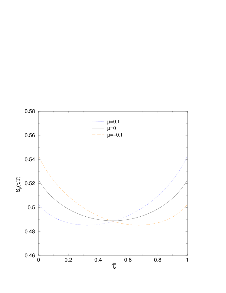
Figure 4: Plots of $S_{\mu}(\tau,T)$ vs. $\tau$ obtained from Eq. (24) for three different values of the drift $\mu=0.1$, $\mu=0$ and $\mu=-0.1$. We have set $T=1$ and $\sigma=1$. The symmetry $S_{\mu}(\tau,T)=S_{-\mu}(T-\tau,T)$ is evident.

Optimal Time $\tau^{*}$: To find the optimal time $\tau^{*}$ we need to minimize $r_{\mu}(\tau,T)$, i.e., maximize $S_{\mu}(\tau,T)$ with respect to $\tau\in[0,T]$. It is evident from Fig. 4 and also from the expression of $S_{\mu}(\tau,T)$ that for all values of $\mu$, $S_{\mu}(\tau,T)$ has two local maxima at the endpoints of the interval $[0,T]$, i.e., respectively at $\tau=0$ and $\tau=T$. However, for $\mu>0$, the maximum at $\tau=T$ has a larger value implying that for $\mu>0$, $\tau^{*}=T$. By the symmetry manifest in $S_{\mu}(\tau,T)=S_{-\mu}(T-\tau,T)$ it follows that for $\mu<0$, the maximum at $\tau=0$ has a higher value implying $\tau^{*}=0$ for $\mu<0$. Exactly at $\mu=0$, both local maxima at $\tau=0$ and $\tau=T$ have the same value ($S_{0}(\tau,T)$ is completely symmetric around the midpoint $\tau=T/2$) implying that for $\mu=0$, both $\tau^{*}=0$ and $\tau^{*}=T$ are optimal.

The optimal value $S_{\mu}(\tau^{*},T)$ is actually easier to evaluate since for $\tau=0$ or $\tau=T$ (at the end-points), the integral in Eq. (24) can be carried out explicitly. Omitting details of this integration, we get the following expression for the optimal relative error for all $\mu$

$$r(\tau^{*},T) = 1-S_{\mu}(\tau^{*},T)$$ (26)

$$= 1-\frac{|\mu|}{2|\mu|+\sigma^{2}}\,{\rm erfc}\left(-\frac{|\mu|}{\sigma}\sqrt{\frac{T}{2}}\right)-\frac{\sigma^{2}+|\mu|}{\sigma^{2}+2|\mu|}\,\exp\left[-\left(|\mu|+\frac{\sigma^{2}}{2}\right)\,T\right]\,{\rm erfc}\left(\left(\frac{|\mu|}{\sigma^{2}}+1\right)\sqrt{\frac{\sigma^{2}T}{2}}\right).$$

Note that the optimal relative error is evidently a symmetric function of $\mu$ as manifest in the above result.

In the preceeding paper SXZ , Shiryaev, Xu and Zhou also obtained an expression of the optimal relative error $r(\tau^{*},T)$ by a completely different method. Their notations are slightly different from above. In their notation, $\mu=(\alpha-1/2)\sigma^{2}$ and also their result for $r(\tau^{*},T)$ is in terms of the probability distribution of a Gaussian random variable with zero mean and unit variance, $\Phi(x)=\frac{1}{\sqrt{2\pi}}\int_{-\infty}^{x}e^{-u^{2}/2}du$ which is related to the complimentary error function via

$$\Phi(x)=\frac{1}{2}\,{\rm erfc}\left(-\frac{x}{\sqrt{2}}\right).$$ (27)

However, their method allows them to obtain an explicit expression for the optimal relative error only in the range $\alpha\geq 1/2$ (i.e., $\mu\geq 0$) and $\alpha\leq 0$ (i.e., $\mu\leq-\sigma^{2}/2$). In these ranges, their expressions for the optimal relative error (Eqs. (9) and (11) in SXZ ) reduce precisely to our compact result in Eq. (26), upon identifying $\mu=(\alpha-1/2)\sigma^{2}$ and $\Phi(x)$ as in Eq. (27). However, they do not have any result in the range $0<\alpha<1/2$, i.e., for $-\sigma^{2}/2<\mu<0$. In contrast, our result in Eq. (26) is valid for all $\mu$ (and hence for all $\alpha$) and is therefore more general. In addition, their method somehow does not detect the symmetry of $r(\tau^{*},T)$ under $\mu\to-\mu$ which is manifest in our path integral approach.

V The exact distribution of the time $t_{m}$ of the occurrence of the maximum for a Brownian motion with drift $\mu$

Minimizing the relative error $r(\tau,T)$ with respect to $\tau$ is one way of estimating the optimal time $\tau^{*}$ at which one should sell a stock over a fixed investment time horizon $T$, as explained above. Another alternative and direct measure would be to first derive the probability density $p(t_{m},T)$ of the time $t_{m}$ at which the maximum $M_{T}$ of a stock price over $[0,T]$ actually occurs. This density $p(t_{m},T)$ will typically have a peak (or more peaks). The value of $t_{m}=t^{*}$ at which the strongest peak of $p(t_{m},T)$ occurs can then be taken as an alternative measure for the optimal time to sell a stock, since the maximum of the price is most likely to occur at $t_{m}=t^{*}$.

In this section, we compute exactly the density $p_{\mu}(t_{m},t)$ of $t_{m}$ for a Brownian motion $x(t)$ with drift $\mu$. Since the stock price $P_{t}=\exp[x(t)]$ is just the exponential of $x(t)$ under the Black-Scholes scenario, the maximum $M_{T}$ of the stock price $P_{t}$ occurs exactly at the same time $t_{m}$ where $x(t)$ itself achieves its maximum. For the case $\mu=0$, the density $p_{0}(t_{m},T)$ was computed by Lévy Levy and is given by the derivative of an arcsine form, i.e.,

$$p_{0}(t_{m},T)=\frac{1}{\pi}\,\frac{1}{\sqrt{t_{m}(T-t_{m})}};\quad\,0\leq t_{m}\leq T$$ (28)

Recently, using an appropriate path integral method, the density of $t_{m}$ was computed exactly for a Brownian motion up to its first-passage time  RM and also for a variety of constrained Brownian motions such as Brownian excursions, Brownian bridges, Brownian meanders etc. MRKY . Here we adapt this path integral method to compute the density $p_{\mu}(t_{m},T)$ for a Brownian motion with arbitrary drift $\mu$.

To compute the density $p_{\mu}(t_{m},T)$ the strategy would be to first compute the joint density of $t_{m}$ as well as the maximum $\tilde{M}_{T}=m$ itself, i.e., $p_{\mu}(t_{m},m,T)$ and then integrate over $m$ to obtain the marginal density, $p_{\mu}(t_{m},T)=\int_{0}^{\infty}p_{\mu}(t_{m},m,T)\,dm$. The joint density $p_{\mu}(t_{m},m,t)$ is the proportional to the sum of the statistical weights of all paths that start at the origin $x(0)=0$, reaches the value $x(t_{m})=m$ for the first-time at $t=t_{m}$ and then stays below the level $m$ at all subsequent times up to $T$,i.e., in the interval $[t_{m},T]$. To enforce the conditions that $x(t)<m$ in the two intervals $t\in[0,t_{m}]$ and $t\in[t_{m},T]$ and that exactly at $t_{m}$ the path reaches $x(t_{m})=m$, poses a problem for a continuous-time Brownian motion. This is because if a Brownian motion crosses a level $m$ at a given time $t_{m}$ then it must cross and re-cross the same level $m$ an infinite number of times in the vicinity of $t=t_{m}$. Hence it is impossible to enforce the above constraints simultaneously for a continuous-time Brownian motion. Note that for lattice random walks this does not pose any problem. To get around this difficulty with the continuous-time Brownian motion, one introduces a small cut-off $\epsilon$ RM ; MRKY , i.e., one assumes that the path, starting at $x(0)=0$ reaches the level $m-\epsilon$ at time $t_{m}$, staying below $m$ for all $0\leq t<t_{m}$ and then starting at $m-\epsilon$ at $t=t_{m}$ stays below the level $m$ for all $t_{m}<t\leq T$ (see Fig. 5 for such a realization). Finally one takes the limit $\epsilon\to 0$ at the end of the calculation.

Figure 5: A realization of the drifted Brownian motion $x(t)$ in $t\in[0,T]$, starting at $x(0)=0$, reaching $x(t_{m})=m-\epsilon$ at $t=t_{m}$ and staying below the level $m$ for all $0\leq t\leq T$.

Comparing Figs. (2) and (5), it is clear that the paths that contribute to the joint probability density $p_{\mu}(t_{m},m,T|\epsilon)$ are identical to those that contribute to $F_{\mu}(x,m,\tau)$ with the replacements $x=m-\epsilon$ and $\tau=t_{m}$ in Eq. (17), i.e., $p_{\mu}(t_{m},m,T|\epsilon)\propto F_{\mu}(m-\epsilon,m,t_{m})$. Substituting $x=m-\epsilon$ and $\tau=t_{m}$ in Eq. (17) and taking the $\epsilon\to 0$ limit we find, to leading order in $\epsilon$,

$$p_{\mu}(t_{m},m,T|\epsilon)\xrightarrow[\epsilon\to 0]{}A\,\epsilon^{2}\,\frac{me^{-(m-\mu t_{m})^{2}/{2\sigma^{2}\,t_{m}}}}{\sqrt{2\pi\,\sigma^{6}\,t_{m}^{3}}}\,\left[\frac{2}{\sqrt{2\pi\sigma^{2}(T-t_{m})}}\,e^{-\mu^{2}(T-t_{m})/{2\sigma^{2}}}-\frac{\mu}{\sigma^{2}}\,{\rm erfc}\left(\frac{\mu}{\sigma}\sqrt{\frac{T-t_{m}}{2}}\right)\right]$$ (29)

where the constant of proportionality $A$, which is function of $\epsilon$, is determined from the normalization, $\int_{0}^{T}dt_{m}\int_{0}^{\infty}dm\,p_{\mu}(t_{m},m,T|\epsilon\to 0)=1$. This fixes $A=\sigma^{2}/{\epsilon^{2}}$. Integrating $p_{\mu}(t_{m},m,T)$ (now the cut-off $\epsilon$ has been set to $0$) over $m$ finally gives the marginal density $p_{\mu}(t_{m},T)$ in a closed form

$$p_{\mu}(t_{m},T)=\frac{1}{\pi\sqrt{t_{m}(T-t_{m})}}\,h(t_{m},\mu)\,h(T-t_{m},-\mu)$$ (30)

where

$$h(t_{m},\mu)=\exp\left(-\frac{\mu^{2}t_{m}}{2\sigma^{2}}\right)+\frac{\mu}{\sigma}\,\sqrt{\frac{\pi t_{m}}{2}}\,{\rm erfc}\left(-\frac{\mu}{\sigma}\sqrt{\frac{t_{m}}{2}}\right).$$ (31)

The density $p_{\mu}(t_{m},T)$ given in Eqs. (30) and (31) is the main result of this section. Evidently, for $\mu=0$, one recovers from this the well known arcsine result of Lévy in Eq. (28). Note that the density $p_{\mu}(t_{m},T)$ also has a symmetry similar to that in Eq. (25) namely

$$p_{\mu}(t_{m},T)=p_{-\mu}(T-t_{m},T).$$ (32)

This symmetry is also evident in Fig. 6 where we plot the density $p_{\mu}(t_{m},T)$ in Eq. (30) for $\mu=1$, $\mu=0$ and $\mu=-1$ upon setting $T=1$ and $\sigma=1$.

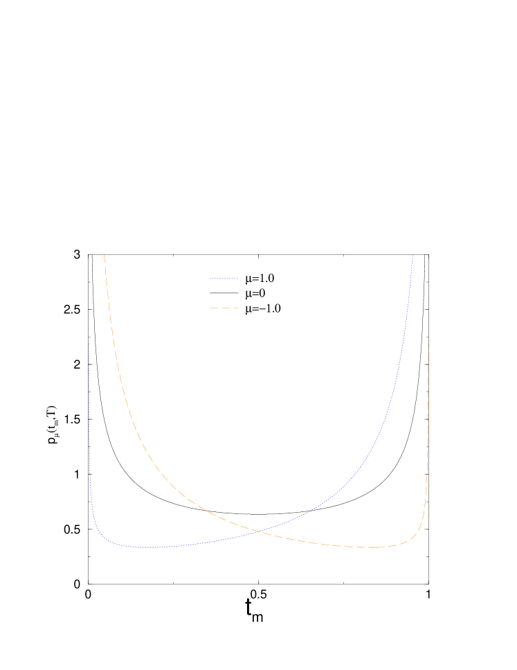
Figure 6: Plots of $p_{\mu}(t_{m},T)$ vs. $t_{m}$ for three different values of the drift $\mu=1.0$, $\mu=0$ and $\mu=-1.0$. We have set $T=1$ and $\sigma=1$. The symmetry $p_{\mu}(t_{m},T)=p_{-\mu}(T-t_{m},T)$ is evident.

We note from Eq. (30) as well as from Fig. 6 that for all values of $\mu$, the density $p_{\mu}(t_{m},T)$ has two peaks (actually has square root divergences) at the two end points $t_{m}=0$ and $t_{m}=T$,

$$p_{\mu}(t_{m}\to 0,T) \approx \frac{A_{\mu}(T)}{\sqrt{t_{m}}}$$ (33)

$$p_{\mu}(t_{m}\to T,T) \approx \frac{A_{-\mu}(T)}{\sqrt{T-t_{m}}}$$ (34)

where the amplitude

$$A_{\mu}(T)=\frac{1}{\pi\sqrt{T}}\,\left[\exp\left(-\frac{\mu^{2}T}{2\sigma^{2}}\right)-\frac{\mu}{\sigma}\,\sqrt{\frac{\pi T}{2}}\,{\rm erfc}\left(\frac{\mu}{\sigma}\sqrt{\frac{T}{2}}\right)\right].$$ (35)

However, for $\mu>0$, the divergence at $t_{m}=T$ is stronger than that at $t_{m}=0$ since $A_{-\mu}(T)>A_{\mu}(T)$. On the other hand, for $\mu<0$, the opposite is true. At $\mu=0$, both ends have the same divergences as the density is completely symmetric around $t_{m}=T/2$. Thus, we conclude that the maximum of the Brownian motion with drift $\mu$ is most likely to occur at $t_{m}=T$ for $\mu>0$, at $t_{m}=0$ for $\mu<0$, and for $\mu=0$ both $t_{m}=0$ and $t_{m}=T$ are equally likely. This then leads us to identify the optimal time $\tau^{*}$ to sell the stock (within the black-Scholes economy model) to be $\tau^{*}=T$ for $\mu>0$, $\tau^{*}=0$ for $\mu<0$, and $\tau^{*}=0,T$ (equally likely) for $\mu=0$. Thus, based on the analysis of the density $p_{\mu}(t_{m},T)$ we draw the same conclusion as was obtained from the optimization of the relative error in the previous sections.

References

(1) A. Shiryaev, Z Xu, and X.Y. Zhou, Thou Shalt Buy and Hold, Quantitative Finance (2008),
preceeding paper.
(2) M. Dai, H. Jin, Y. Zhong, X.Y. Zhou, working paper, 2008.
(3) S.N. Majumdar, Brownian Functionals in Physics and Computer Science, Current
Science, 89, 2076 (2005) (also available at cond-mat/0510064).
(4) S.N. Majumdar, J. Randon-Furling, M.J. Kearney, and M. Yor, On the Time to Reach
Maximum for a Variety of Constrained Brownian Motions, J. Phys. A: Math. Theor. 41, 365005 (2008).
(5) W. Feller, An Introduction to Probability Theory and Its
Applications, vol-I and II (Wiley, New York, 1968).
(6) S. Redner, A Guide to First-passage Processes
(Cambridge University Press, Cambridge 2001).
(7) P. Lévy, Sur Certains Processus Stochastiques Homogènes, Composition
Mathematica, 7, 283 (1939).
(8) J. Randon-Furling and S.N. Majumdar, Distribution of the Time at which the
Deviation of a Brownian Motion is Maximum before its
First-passage Time, Journal of Stat. Mech.: Th. and Exp. P10008 (2007).