Target Localization Accuracy Gain in MIMO Radar Based Systems

Abstract

This paper presents an analysis of target localization accuracy, attainable by the use of MIMO (Multiple-Input Multiple-Output) radar systems, configured with multiple transmit and receive sensors, widely distributed over a given area. The Cramer-Rao lower bound (CRLB) for target localization accuracy is developed for both coherent and non-coherent processing. Coherent processing requires a common phase reference for all transmit and receive sensors. The CRLB is shown to be inversely proportional to the signal effective bandwidth in the non-coherent case, but is approximately inversely proportional to the carrier frequency in the coherent case. We further prove that optimization over the sensors’ positions lowers the CRLB by a factor equal to the product of the number of transmitting and receiving sensors. The best linear unbiased estimator (BLUE) is derived for the MIMO target localization problem. The BLUE’s utility is in providing a closed form localization estimate that facilitates the analysis of the relations between sensors locations, target location, and localization accuracy. Geometric dilution of precision (GDOP) contours are used to map the relative performance accuracy for a given layout of radars over a given geographic area.

I Introduction

I-A Background and Motivation

Research in MIMO radar has been growing as evidenced by an increasing body of literature [1]-[18]. Generally speaking, MIMO radar systems employ multiple antennas to transmit multiple waveforms and engage in joint processing of the received echoes from the target. Two main MIMO radar architectures have evolved: with colocated antennas and with distributed antennas. MIMO radar with colocated antennas makes use of waveform diversity [2, 4, 12, 14, 15], while MIMO radar with distributed antenna takes advantage of the spatial diversity supported by the system configuration [1, 3, 5, 13]. MIMO radar systems have been shown to offer considerable advantages over traditional radars in various aspects of radar operation such as the detection of slow moving targets [17, 8], the ability to identify and separate multiple targets [10, 11], and in the estimation of target parameters such as direction-of-arrival (DOA) [8, 10], and range-based target localization [18]. In particular, [18] studies target localization with MIMO radar systems utilizing sensors distributed over a wide area.

Conventional localization techniques include time-of-arrival (TOA), time-difference-of-arrival (TDOA), and direction-of-arrival (DOA) based schemes. MIMO radar system with colocated antenna can perform DOA estimation of targets in the far-field, in which case, the received signal has a planar wavefront. In this class of systems, extensive research has focused on waveform optimization. In [7, 14, 15] the signal vector transmitted by a MIMO radar system is designed to minimize the cross-correlation of the signals bounced from various targets to improve the parameter estimation accuracy in multiple target schemes. Some of the waveform optimization techniques suggested in [16] are based on the Cramer-Rao lower bound (CRLB) matrix [19],[20]. The CRLB is known to provide a tight bound on parameter estimation for high signal-to-noise ratio (SNR). Several design criteria are considered, such as minimizing the trace, determinant, and the largest eigenvalue of the CRLB matrix, concluding that minimizing the trace of the CRLB gives a good overall performance in terms of lowering the CRLB. In [9], a CRLB evaluation of the achievable angular accuracy is derived for linear arrays with orthogonal signals. The use of orthogonal signals is shown to provide better accuracy than correlated signals. For low SNR scenarios, the Barankin bound is derived in [10], demonstrating that the use of orthogonal signals results in a lower SNR threshold for transitioning into the region of higher estimation error.

MIMO radar systems with widely spread antennas take advantage of the geographical spread of the deployed sensors. The multiple propagation paths, created by the transmitted waveforms and echoes from scatterers in their paths support target localization through either direct or indirect multilateration. With direct multilateration, the observations collected by the sensors are jointly processed to produce the localization estimate. With indirect multilateration, the TOAs are estimated first, and the localization is subsequently estimated from the TOAs. The observations and processing can also be classified as either non-coherent or coherent. The distinction between the two modes relies on the need for mere time synchronization between the transmitting and receiving radars in the non-coherent case, versus the need for both time and phase synchronization in the coherent case. Note that our coherent/non-coherent terminology is limited to the processing for localization. Thus, a transmitted signal may have in-phase and quadrature components, yet the localization processing is non-coherent if it utilizes only information in the signal envelope. In the sequel, we evaluate the performance of localization utilizing both coherent and non-coherent processing.

MIMO radar systems belongs to the class of active localization systems, where the signal usually travels a round trip, i.e. the signal transmitted by one sensor in a radar system is reflected by the target and measured by the same or a different sensor. Traditional single-antenna radar systems, performing active range-based measurements, are well known in literature [21]-[25]. The target range is computed from the time it takes for the transmitted signal to get to the target plus the travelling time of the reflected signal back to the sensor. The range estimation accuracy is directly proportional to the mean squared error (MSE) of the time delay estimation and is shown to be inversely proportional to the signal effective bandwidth [21]. A first study of the localization accuracy capability of MIMO radar systems is provided in [18], where the Fisher information matrix (FIM) is derived for the case of orthogonal signals with coherent processing and widely separated antennas. The CRLB is analyzed numerically, pointing out the dependency of the accuracy on the signal carrier frequency in the coherent case, and its reliance on the relative locations of the target and sensors. In [18], it is observed that the CRLB is a function of the number of transmitting and receiving sensors, however an analytical relation is not developed. The high accuracy capability of coherent processing is illustrated by the use of the ambiguity function (AF). Active range-based target localization techniques are also used in multistatic radar systems, proposed in [26]. The TOA of a signal transmitted by a single transmit radar, reflected by the target and received at multiple receive antennas is used in the localization process. It is observed that increasing the number of sensors improves localization performance, yet an exact relation is not specified. This paper addresses deficiencies in the literature by obtaining closed-form expressions of the CRLB for both coherent and non-coherent cases.

Geolocation techniques has been the subject of extensive research. Geolocation belongs to the class of passive localization systems, where the signal travels one-way. Since these passive measurement systems employ multiple sensors, further evaluation of existing results for geolocation systems might provide insightful for the active case. In wireless communication, passive measurements are used by multiple base stations for localization of a radiating mobile phone. The localization accuracy performance is evaluated in [27]. It is shown that the localization accuracy is inversely proportional to the signal effective bandwidth as it does in the active localization case. Moreover, the accuracy estimation is shown to be dependent on the sensors/base stations locations. In navigation systems, the target makes use of time synchronized transmission from multiple Global Positioning Systems (GPS) to establish its location. In [28, 29], the relation between the transmitting sensors location and the target localization performance is analyzed. GDOP plots are used to demonstrate the dependency of the attainable accuracy on the location of the GPS systems with respect to the target. In an optimal setting of the GPS systems relative to the target position, the best achievable accuracy is shown to be inversely proportional to the square root of the number of participating GPS. In the sequel, we apply the GDOP metric to evaluate the localization performance of MIMO radar.

I-B Main Contributions

The main contributions of this paper are:

1. The CRLB of the target localization estimation error is developed for the general case of MIMO radar with multiple waveforms transmission. The analytical expressions of the CRLB are derived for the case of orthogonal waveforms with non-coherent and coherent observations. The non-coherent case is used as benchmark for evaluating the performance of the system with coherent observations.

2. It is shown that the CRLB expressions for both the non-coherent and coherent cases can be factored into two terms: a term incorporating the effect of bandwidth and SNR, and another term accounting for the effect of sensor placement.

3. The CRLB of the standard deviation of the localization estimate with non-coherent observations is shown to be inversely proportional to the signals averaged effective bandwidth. Dramatically higher accuracy can be obtained from processing coherent observations. In this case, the CRLB is inversely proportional to the carrier frequency. This gain is due to the exploitation of phase information, and is referred to as coherency gain.

4. Formulating a convex optimization problem, it is shown that symmetric deployment of transmitting and receiving sensors around a target is optimal with respect to minimizing the CRLB. The closed form solution of the optimization problem also reveals that optimally placed $M$ transmitters and $N$ receivers reduce the CRLB on the variance of the estimate by a factor $MN/2.$ This is referred to as the MIMO radar gain.

5. A closed form solution is developed for the BLUE of target localization for coherent MIMO radars. It provides a closed form solution and a comprehensive evaluation of the performance of the estimator’s MSE. This estimator provides insight into the relation between sensors locations, target location, and localization accuracy through the use of the GDOP metric. Contour maps of the GDOP, presented in this paper, provide a clear understanding of the mutual relation between a given deployment of sensors and the achievable accuracy at various target locations.

The rest of the paper is organized as follows: The system model is introduced in Section II. In Section III, the CRLB is derived for the general case of multiple transmitted waveforms. Analytical expressions are obtained for the cases of non-coherent and coherent observations with orthogonal signals. Optimization of the CRLB as a function of sensor location is provided in Section IV. The performance of two localization estimators is evaluated in Section V. To establish a better understanding of the relations between the radar geographical spread and the target location, the GDOP metric is introduced in Section V-D. Finally, Section VI concludes the paper.

A comment on notation: vectors are denoted by lower-case bold, while matrices use upper-case bold letters. The superscripts “T” and “H” denote the transpose and Hermitian operators, respectively. Complex conjugate is denoted $\left({}\right)^{\ast}$. Points in the x-y plane are denoted in upper-case $X=\left(x,y\right).$

II System Model

We consider a widely distributed MIMO radar system with $M$ transmitting radars and $N$ receiving radars. The receiving radars may be colocated with the transmitting ones or individually positioned. The transmitting and receiving radars are located in a two dimensional plane $(x,y)$. The $M$ transmitters are arbitrarily located at coordinates $T_{k}=\left(x_{tk},y_{tk}\right),$ $k=1,\ldots,M$, and the $N$ receivers are similarly arbitrarily located at coordinates $R_{\ell}=\left(x_{r\ell},y_{r\ell}\right),$ $\ell=1,\ldots,N.$ The set of transmitted waveforms in lowpass equivalent form is $s_{k}\left(t\right),$ $k=1,\ldots,M,$ where $\int_{\mathcal{T}}\left|s_{k}\left(t\right)\right|^{2}dt=1,$ and $\mathcal{T}$ is the common duration of all transmitted waveforms. The power of the transmitted waveforms is normalized such that the aggregate power transmitted by the sensors is constant, irrespective of the number of transmit sensors. To simplify the notation, the signal power term is embedded in the noise variance term such that the SNR at the transmitter, denoted SNR_t and defined as the transmitted power by a sensor divided by the noise power at a receiving sensor, is set that a desired level. Let all transmitted waveforms be narrowband signals with individual effective bandwidth $\beta_{k}$ defined as $\beta_{k}^{2}=\left[\left(\int_{W_{k}}f^{2}\left|S_{k}\left(f\right)\right|^{2}df\right)/\left(\int_{W_{k}}\left|S_{k}\left(f\right)\right|^{2}df\right)\right]$, where the integration is over the range of frequencies with non-zero signal content $W_{k}$ [21]. We further define the signals averaged effective bandwidth or rms bandwidth as $\beta^{2}=\frac{1}{M}\sum_{k=1}^{M}\beta_{k}^{2}$ and the normalized bandwidth terms as $\beta_{R_{k}}=\beta_{k}/\beta$. The signals are narrowband in the sense that for a carrier frequency of $f_{c},$ the narrowband signal assumption implies $\beta_{k}^{2}/$ $f_{c}^{2}\ll 1$ and $\beta^{2}/$ $f_{c}^{2}\ll 1$.

The target model developed here generalizes the model in [21] to a near-field scenario and distributed sensors. In Skolnik’s model [21], the returns of individual point scatterers have fixed amplitude and phase, and are independent of angle. For a moving target, the composite return fluctuates in amplitude and phase due to the relative motion of the scatterers. When the motion is slow, and the composite target return is assumed to be constant over the observation time, the target conforms to the classical Swerling case I model. We now proceed to generalize this model to a target observed by a MIMO radar with distributed sensors. Assume an extended target, composed of a collection of $Q$ individual point scatterers located at coordinates $X_{q}=\left(x_{q},y_{q}\right),$ $q=1,\ldots,Q$. The amplitudes $\zeta_{q}$ of the point scatterers are assumed to be mutually independent. The pathloss and phase of a signal reflected by a scatterer, when measured with respect to a transmitted signal $s_{k}\left(t\right),$ are functions of the path transmitter-scatterer-receiver. Let ${\tau_{\ell k}}\left(X_{q}\right)$ denote the propagation time from transmitter $k,$ to scatterer $q,$ to receiver $\ell,$

$${\tau_{\ell k}}\left(X_{q}\right)=\frac{1}{c}\left(\sqrt{\left(x_{tk}-x_{q}\right)^{2}+\left(y_{tk}-y_{q}\right)^{2}}+\sqrt{\left(x_{r\ell}-x_{q}\right)^{2}+\left(y_{r\ell}-y_{q}\right)}\right),$$ (1)

where $c$ is the speed of light. Our signal model assumes that the sensors are located such that variations in the signal strength due to different target to sensor distances can be neglected, i.e., the model accounts for the effect of the sensors/target localizations only through time delays (or phase shifts) of the signals. The common path loss term is embedded in $\zeta_{q}.$ The baseband representation for the signal received at sensor $\ell$ is:

$$r_{\ell}\left(t\right)=\sum_{k=1}^{M}\sum_{q=1}^{Q}\zeta_{q}\exp\left({-j2\pi f_{c}\tau_{\ell k}}\left(X_{q}\right)\right)s_{k}\left(t-\tau_{\ell k}\left(X_{q}\right)\right)+w_{\ell}(t),$$ (2)

where the term ${2\pi f_{c}\tau_{\ell k}}\left(X_{q}\right)\$is the phase of a signal transmitted by sensor $k,$ reflected by scatterer $q$ located at $X_{q},$ and received by sensor $\ell.$ Phases are measured relative to a common phase reference assumed to be available at the transmitters and receivers. The term $w_{\ell}\left(t\right)$ is circularly symmetric, zero-mean, complex Gaussian noise, spatially and temporally white with autocorrelation function $\sigma_{w}^{2}\delta\left(\tau\right)$. The noise term is set $\sigma_{w}^{2}=1/$SNR_t, where SNR_t is measured at the transmitter. SNR_t is normalized such that the aggregate transmitted power is independent of the number of transmitting sensors. The SNR at the receiver, due to a scatterer with amplitude $\zeta_{q}$, is SNR${}_{r}=\left|\zeta_{q}\right|^{2}$SNR${}_{t}.$ Signals reflected from the target combine at each of the receive antennas. For example, the resultant signal at receive antenna $\ell$ is given by

$$\sum_{q=1}^{Q}\zeta_{q}s_{k}\left(t-\tau_{\ell k}\left(X_{q}\right)\right)\exp\left({-j2\pi f_{c}\tau_{\ell k}}\left(X_{q}\right)\right)\thickapprox\zeta^{\prime}s_{k}\left(t-\tau_{\ell k}\left(X^{\prime}\right)\right)\exp\left({-j2\pi f_{c}\tau_{\ell k}}\left(X^{\prime}\right)\right),$$ (3)

where $\zeta^{\prime}$ and $\left({2\pi f_{c}\tau_{\ell k}}\left(X^{\prime}\right)\right)$ are respectively the amplitude and phase given by

$$\zeta^{\prime}=\left[\left(\sum_{q=1}^{Q}\zeta_{q}\cos\left({2\pi f_{c}\tau_{\ell k}}\left(X_{q}\right)\right)\right)^{2}+\left(\sum_{q=1}^{Q}\zeta_{q}\sin\left({2\pi f_{c}\tau_{\ell k}}\left(X_{q}\right)\right)\right)^{2}\right]^{1/2},$$ (4)

and

$${2\pi f_{c}\tau_{\ell k}}\left(X^{\prime}\right)=\tan^{-1}\frac{\sum_{q=1}^{Q}\zeta_{q}\sin\left({2\pi f_{c}\tau_{\ell k}}\left(X_{q}\right)\right)}{\sum_{q=1}^{Q}\zeta_{q}\cos\left({2\pi f_{c}\tau_{\ell k}}\left(X_{q}\right)\right)}.$$ (5)

In obtaining (3), we invoked the narrowband assumption $s_{k}\left(t-\tau_{\ell k}\left(X_{q}\right)\right)\thickapprox s_{k}\left(t-\tau_{\ell k}\left(X^{\prime}\right)\right)$, for all scatterers, namely that the change in the lowpass equivalent signals across the target is negligible. It follows from this discussion that the extended target is represented by a point scatterer of amplitude $\zeta^{\prime}$ and time delays ${\tau_{\ell k}}\left(X^{\prime}\right),$ where all the quantities are unknown.

While this target model is completely adequate for our needs, it is possible to extend it slightly, at little cost. Assume a constant time offset error $\Delta\tau$ at the receivers. Further, assume that the error is small such that it does not impact the signal envelope, but it does impact the phase. Then we can write the time delays $\tau_{\ell k}\left(X^{\prime}\right)=\tau_{\ell k}\left(X\right)+\Delta\tau$ for some location $X=\left(x,y\right).$ The target model (3) can now be expressed

$$\zeta^{\prime}s_{k}\left(t-\tau_{\ell k}\left(X^{\prime}\right)\right)\exp\left({-j2\pi f_{c}\tau_{\ell k}}\left(X^{\prime}\right)\right)\thickapprox\zeta s_{k}\left(t-\tau_{\ell k}\left(X\right)\right)\exp\left({-j2\pi f_{c}\tau_{\ell k}}\left(X\right)\right),$$ (6)

where $\zeta=\zeta^{\prime}e^{-j2\pi f_{c}\Delta\tau}$ and the narrowband assumption was invoked once more. The composite target of (3) is then equivalent to a point scatterer of complex amplitude $\zeta$ and time delays ${\tau_{\ell k}}\left(X\right).$ For simplicity, the following notation is used: ${\tau_{\ell k}=\tau_{\ell k}}\left(X\right)$. The signal model (2) becomes

$$r_{\ell}\left(t\right)=\sum_{k=1}^{M}\zeta\exp\left({-j2\pi f_{c}\tau_{\ell k}}\right)s_{k}\left(t-\tau_{\ell k}\right)+w_{\ell}(t).$$ (7)

We define the vector of received signals as $\mathbf{r=}\left[r_{1},r_{2},...,r_{N}\right]^{T}$ for later use. The radar system’s goal is to estimate the target location $X=\left(x,y\right).$ The target location can be estimated directly, for example by formulating the maximum likelihood estimate (MLE) associated with (7). Alternatively, an indirect method is to estimate first the time delays ${\tau_{\ell k}}.$ Subsequently, the target location can be computed from the solution to a set of equations of the form (1), viz.,

$${\tau_{\ell k}}=\frac{1}{c}\left(\sqrt{\left(x_{tk}-x\right)^{2}+\left(y_{tk}-y\right)^{2}}+\sqrt{\left(x_{r\ell}-x\right)^{2}+\left(y_{r\ell}-y\right)^{2}}\right).$$ (8)

The unknown complex amplitude $\zeta$ is treated as a nuisance parameter in the estimation problem.

Let the unknown target location $X=\left(x,y\right),$ unknown time delays delays $\tau_{\ell k}$, and unknown target complex amplitude $\zeta=\zeta^{R}+j\zeta^{I},$ where the notation specifies the real and imaginary components of $\zeta.$

We refer to the processing for estimating the target location as non-coherent or coherent. The received signal introduced in (7) is adequate for the coherent case, where the transmitting and receiving radars are assumed to be both time and phase synchronized. As such, the time delays information, $\tau_{\ell k}$, embedded in the phase terms may be exploited in the estimation process by matching both amplitude and phase at the receiver end. In contrast, non-coherent processing estimates the time delays $\tau_{\ell k}$ from variations in the envelope of the transmitted signals $s_{k}\left(t\right).$ A common time reference is required for all the sensors in the system. In this case, the transmitting radars are not phase synchronized and therefore the received signal model is of the form:

$$r_{\ell}\left(t\right)=\sum_{k=1}^{M}\alpha_{\ell k}s_{k}\left(t-\tau_{\ell k}\right)+w_{\ell}(t),$$ (9)

where the complex amplitude terms $\alpha_{\ell k}$ integrate the effect of the phase offsets between the transmitting and receiving sources and the target impact on the phase and amplitude of the transmitted signals. These elements are treated as unknown complex amplitudes, where $\alpha_{\ell k}=\alpha_{\ell k}^{R}+j\alpha_{\ell k}^{I}$. We define the following vector notations:

$$\begin{array}[c]{c}\mathbf{\alpha}=[\alpha_{11},\alpha_{12},...,\alpha_{\ell k},...,\alpha_{MN}]^{T},\end{array}$$ (11)

$$\begin{array}[c]{cc}\mathbf{\alpha}^{R}=\operatorname{Re}\left(\mathbf{\alpha}\right);&\mathbf{\alpha}^{I}=\operatorname{Im}\left(\mathbf{\alpha}\right),\end{array}\$$ (13)

where $\operatorname{Re}\left(\mathbf{\cdot}\right)$ and $\operatorname{Im}\left(\mathbf{\cdot}\right)$ denote the real and imaginary parts of a complex-valued vector/matrix.  

III  Localization CRLB

The CRLB provides a lower bound for the MSE of any unbiased estimator for an unknown parameter(s). Given a vector parameter $\mathbf{\theta},$ constituted of elements $\theta_{i},$ the unbiased estimate $\widehat{\theta}_{i}$ satisfies the following inequality [19]:

$$\operatorname{var}\left(\widehat{\theta}_{i}\right)\geq\left[\mathbf{J}^{-1}\left(\mathbf{\theta}\right)\right]_{ii},\text{ \ \ }i=1,2,...\ \text{\ }$$ (14)

where $\left[\mathbf{J}^{-1}\left(\mathbf{\theta}\right)\right]_{ii}$ are the diagonal elements of the Fisher Information matrix (FIM) $\mathbf{J}\left(\mathbf{\theta}\right)$. The FIM is given by:

$$\mathbf{J}\left(\mathbf{\theta}\right)=E_{\mathbf{\theta}}\left[\frac{\partial}{\partial\mathbf{\theta}}\log p\left(\mathbf{r|\theta}\right)\left(\frac{\partial}{\partial\mathbf{\theta}}\log p\left(\mathbf{r|\theta}\right)\right)^{T}\right],$$ (15)

where $p\left(\mathbf{r|\theta}\right)$ is the joint probability density function (pdf) of $\mathbf{r}$ conditioned on $\mathbf{\theta}$.

The CRLB is then defined:

$$\mathbf{C}_{CRLB}=\left[\mathbf{J}\left(\mathbf{\theta}\right)\right]^{-1}.$$ (16)

Sometime, it is easier to compute the FIM with respect to another vector $\mathbf{\psi,}$ and apply the chain rule to derive the original $\mathbf{J}\left(\mathbf{\theta}\right).$ In our case, since the received signals in both (7) and (9) are functions of the time delays, $\tau_{\ell k},$ and the complex amplitudes, by the chain rule, $\mathbf{J}\left(\mathbf{\theta}\right)$ can be expressed in the alternative form [19]:

$$\mathbf{J}\left(\mathbf{\theta}\right)=\mathbf{PJ}\left(\mathbf{\psi}\right)\mathbf{P}^{T},$$ (17)

where $\mathbf{\psi}$ is a vector of unknown parameters, and it incorporates the time delays. Matrix $\mathbf{J}\left(\mathbf{\psi}\right)$ is the FIM with respect to $\mathbf{\psi,}$ and matrix $\mathbf{P}$ is the Jacobian:

$$\mathbf{P}{\small=\frac{\partial\mathbf{\psi}}{\partial\mathbf{\theta}}.}$$ (18)

From this point onward, we develop the CRLB for the case of non-coherent and coherent processing, separately.

III-A Non-coherent Processing CRLB

For non-coherent Processing, there is no common phase reference among the sensors. Consequently, the complex-valued terms $\alpha_{lk}$ incorporate phase offsets among sensors and the effect of the target on the phase and complex amplitude, following the definitions in (11). The vectors of unknown parameters is defined:

$$\mathbf{\theta}_{nc}=\left[x,y,\mathbf{\alpha}^{R}\mathbf{,\alpha}^{I}\right]^{T}.$$ (19)

The process of localization by non-coherent processing depends on time delay estimation of the signals observed at the receive sensors and also on the location of the sensors. To gain insight into how each of the factors affects the performance of localization, we utilize the form of the FIM given in (17). We define the vector of unknown parameters:

$$\mathbf{\psi}_{nc}=\left[\mathbf{\tau},\mathbf{\alpha}^{R}\mathbf{,\alpha}^{I}\right]^{T},$$ (20)

where $\mathbf{\alpha}$ is given in (11) and $\mathbf{\tau=}$ $\left[\tau_{11},\tau_{12},...,\tau_{\ell k},...,\tau_{MN}\right]^{T}$. We are interested only in the estimation of $x$ and $y$, while $\mathbf{\alpha}^{R}\mathbf{,}$ $\mathbf{\alpha}^{I}$ act as nuisance parameters in the estimation problem.

Given a set of known transmitted waveforms $s_{k}\left(t-\tau_{\ell k}\right)$ parameterized by the unknown time delays $\tau_{\ell k},$ which in turn are a function of the unknown target location $X=\left(x,y\right)$, the conditional, joint pdf of the observations at the receive sensors, given by (9), is then:

$$p\left(\mathbf{r}|\mathbf{\psi}_{nc}\right)\varpropto\exp\left\{-\frac{1}{\sigma_{w}^{2}}\overset{N}{\underset{\ell=1}{\sum}}\int\limits_{T}\left|r_{\ell}(t)-\overset{M}{\underset{k=1}{\sum}}\alpha_{\ell k}s_{k}\left(t-\tau_{\ell k}\right)\right|^{2}dt\right\}.$$ (21)

The matrix $\mathbf{P}_{nc}$ for (19) and (20), to be used in (17), is defined as:

$$\mathbf{P}_{nc}=\frac{\partial\mathbf{\psi}_{nc}}{\partial\mathbf{\theta}_{nc}}=\left[\begin{array}[c]{ccc}\frac{\partial}{\partial x}\mathbf{\tau}^{T}&\frac{\partial}{\partial x}\left(\mathbf{\alpha}^{R}\right)^{T}&\frac{\partial}{\partial x}\left(\mathbf{\alpha}^{I}\right)^{T}\\ \frac{\partial}{\partial y}\mathbf{\tau}^{T}&\frac{\partial}{\partial y}\left(\mathbf{\alpha}^{R}\right)^{T}&\frac{\partial}{\partial y}\left(\mathbf{\alpha}^{I}\right)^{T}\\ \frac{\partial\mathbf{\tau}}{\partial\mathbf{\alpha}^{R}}&\frac{\partial\mathbf{\alpha}^{R}}{\partial\mathbf{\alpha}^{R}}&\frac{\partial\mathbf{\alpha}^{I}}{\partial\mathbf{\alpha}^{R}}\\ \frac{\partial\mathbf{\tau}}{\partial\mathbf{\alpha}^{I}}&\frac{\partial\mathbf{\alpha}^{R}}{\partial\mathbf{\alpha}^{I}}&\frac{\partial\mathbf{\alpha}^{I}}{\partial\mathbf{\alpha}^{I}}\end{array}\right]_{\left(2MN+2\right)\times 3MN}{\small,}$$ (22)

where $\frac{\partial}{\partial x}\mathbf{\tau}$ is standard notation for taking the derivative with respect to $x$ of each element of $\mathbf{\tau,}$ and $\dfrac{\partial\mathbf{\tau}}{\partial\mathbf{\alpha}^{R}}$ denotes the Jacobian of the vector $\mathbf{\tau}$ with respect to the vector $\mathbf{\alpha}^{R}.$ The subscript denotes the matrix dimensions.

It is not too difficult to show that using (8), the matrix $\mathbf{P}_{nc}$ can be expressed in the form:

$$\mathbf{P}_{nc}={\small-}\frac{1}{c}\left[\begin{array}[c]{cc}\mathbf{H}_{2\times MN}&\mathbf{0}_{2\times 2MN}\\ \mathbf{0}_{2MN\times MN}&\mathbf{I}_{2MN\times 2MN}\end{array}\right]{\small,}$$ (23)

where $\mathbf{0}$ is the all zero matrix, $\mathbf{I}$ is the identity matrix, and $\mathbf{H}\in R^{2\times MN}$ incorporates the derivatives of the time delays in (8) with respect to the $x$ and $y$ parameters. These derivatives result in cosine and sine functions of the angles the transmitting and receiving radars create with respect to the target, incorporating information on the sensors and target locations as follows:

$$\mathbf{H}=\left[\begin{array}[c]{cccc}a_{tx_{1}}+a_{rx_{1}}&a_{tx_{1}}+a_{rx_{2}}&...&a_{tx_{M}}+a_{rxN}\\ b_{tx_{1}}+b_{rx_{1}}&b_{tx_{1}}+b_{rx_{2}}&...&b_{tx_{M}}+b_{rxN}\end{array}\right].$$ (24)

The elements of $\mathbf{H}$ are given by:

$$\begin{array}[c]{ccc}a_{tx_{k}}=\cos\phi_{k};&b_{tx_{k}}=\sin\phi_{k};&k=1,..,M,\\ a_{rx_{\ell}}=\cos\varphi_{\ell};&b_{rx_{\ell}}=\sin\varphi_{\ell};&\ell=1,..,N,\end{array}$$ (27)

$$\begin{array}[c]{cc}\phi_{k}=\tan^{-1}\left(\frac{y-y_{tk}}{x-x_{tk}}\right);&\varphi_{\ell}=\tan^{-1}\left(\frac{y-y_{r\ell}}{x-x_{r\ell}}\right),\end{array}$$ (29)

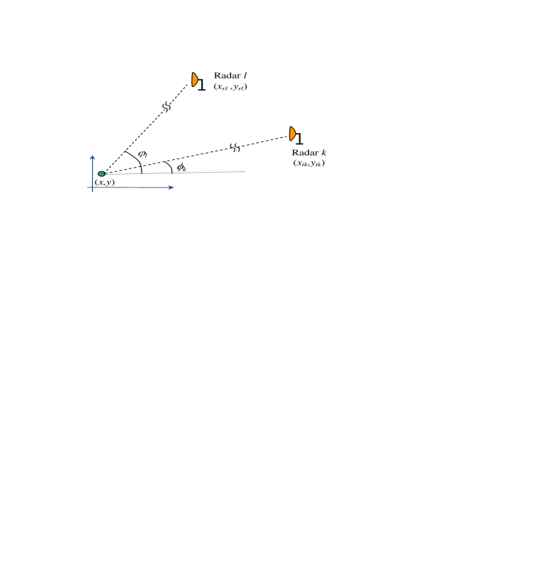
Figure 1: MIMO radar system layout.

where the phase $\phi_{k}$ is the bearing angle of the transmitting sensor $k$ to the target measured with respect to the $x$ axis; the phase $\varphi_{\ell}$ is the bearing angle of the receiving radar $\ell$ to the target measured with respect to the $x$ axis. See illustration in Figure 1. For later use, we apply the following definitions: $\mathbf{\phi}=\left[\phi_{1},\phi_{2},...,\phi_{M}\right]^{T}$, $\mathbf{\varphi}=\left[\varphi_{1},\varphi_{2},...,\varphi_{N}\right]^{T}$, $\mathbf{a}_{tx}=\left[a_{tx_{1}},a_{tx_{2}},...,a_{tx_{M}}\right]^{T}$, $\mathbf{a}_{rx}=\left[a_{rx_{1}},a_{rx_{2}},...,a_{rx_{N}}\right]^{T},$ $\mathbf{b}_{tx}=\left[b_{tx_{1}},b_{tx_{2}},...,b_{tx_{M}}\right]^{T}$ and $\mathbf{b}_{rx}=\left[b_{rx_{1}},b_{rx_{2}},...,b_{rx_{M}}\right]^{T}$.

An expression for the FIM $\mathbf{J}\left(\mathbf{\psi}_{nc}\right),$ is derived in Appendix A, yielding:

$$\mathbf{J}{\small\left(\mathbf{\psi}_{nc}\right)}=\frac{2}{\sigma_{w}^{2}}\left[\begin{array}[c]{cc}\mathbf{S}_{nc}&\mathbf{V}_{nc}\\ \mathbf{V}_{nc}^{T}&\mathbf{\Lambda}_{\alpha}\end{array}\right]_{\left(3MN\right)\times\left(3MN\right)},$$ (30)

with the block matrices $\mathbf{S}_{nc},$ $\mathbf{\Lambda}_{\alpha},$ and $\mathbf{V}_{nc}$ defined in the Appendix A in (111), (116), and (119), respectively.

In order to determine the value of $\mathbf{J}\left(\mathbf{\theta}_{nc}\right),$ we use (30) and (23) in (17), to obtain the following CRLB matrix:

$$\mathbf{C}_{CRLB_{nc}}=\mathbf{J}^{-1}\left(\mathbf{\theta}_{nc}\right)=\frac{c^{2}}{2/\sigma_{w}^{2}}\left[\begin{array}[c]{cc}\mathbf{HS}_{nc}\mathbf{H}^{T}&\mathbf{HV}_{nc}\\ \mathbf{V}_{nc}^{T}\mathbf{H}^{T}&\mathbf{\Lambda}_{\alpha}\end{array}\right]^{-1}.$$ (31)

The CRLB matrix is related to the sensor and target locations through the matrix $\mathbf{H},$ and to the received waveforms correlation functions and its derivatives through the $\mathbf{S}_{nc}$ and $\mathbf{V}_{nc}$ matrices.

III-A1 Orthogonal Waveforms

When the waveforms are orthogonal, (111), (116), and (119) simplify to (120) in Appendix A. This simplification enables to compute the CRLB (31) in closed form. We perform this calculation next.

While the CRLB expresses the lower bound on the variance of the estimate of $\mathbf{\theta}_{nc}=\left[x,y,\mathbf{\alpha}^{R}\mathbf{,\alpha}^{I}\right]^{T}$, we are really interested only in the estimation of $x$ and $y.$ The amplitude terms $\mathbf{\alpha}^{R}$ and $\mathbf{\alpha}^{I}$ serve as nuisance parameters. For the variances of the estimates of $x$ and $y,$ it is sufficient to derive the $2\times 2$ upper left submatrix $\left[\mathbf{C}_{CRLB_{nc}}\right]_{2\times 2}=\left[\left(\mathbf{J}\left(\mathbf{\theta}_{nc}\right)\right)^{-1}\right]_{2\times 2}.$

Proposition 1

The CRLB submatrix $\left[\mathbf{C}_{CRLB_{nc}}\right]_{2\times 2}$ for target localization in the non-coherent case with orthogonal signals is:

$$\left[\mathbf{C}_{CRLB_{nc}}\right]_{2\times 2}{\normalsize=}\frac{c^{2}}{2/\sigma_{w}^{2}}\left(\mathbf{H\mathbf{S}}_{nc}\mathbf{H}^{T}\right)^{-1}.$$ (32)

Proof:

From (120) in Appendix A, we have for terms of (31):

$$\mathbf{S}_{nc} =4\pi^{2}\beta^{2}\left[\operatorname*{diag}(\mathbf{\alpha)B}\operatorname*{diag}(\mathbf{\alpha}^{\ast}\mathbf{)}\right],$$ (33)

$$\mathbf{V}_{nc} =\mathbf{0},$$

$$\mathbf{\Lambda}_{\alpha} =\mathbf{I}_{2MN\times 2MN}.$$

In (33), $\operatorname*{diag}(\mathbf{\alpha})$ denotes a diagonal matrix with the elements of vector $\mathbf{\alpha}$. Matrix $\mathbf{B}=\operatorname*{diag}\left(\mathbf{1}\left[\beta_{R_{1}}^{2},\beta_{R_{2}}^{2},...,\beta_{R_{M}}^{2}\right]\right)$, with $\beta_{R_{k}}$ denoting the normalized elements $\beta_{R_{k}}=\beta_{k}/\beta$, and $\mathbf{1=}\left[1,1,...1\right]^{T}$, $\mathbf{1}\in R^{N\times 1}$. Using (33) in (31), it is easy to see that

$$\left[\mathbf{C}_{CRLB_{nc}}\right]_{2\times 2} =\frac{c^{2}}{2/\sigma_{w}^{2}}\left(\mathbf{H\mathbf{S}}_{nc}\mathbf{H}^{T}\right)^{-1}$$ (34)

$$=\frac{\eta_{nc}}{g_{x_{nc}}g_{y_{nc}}-h_{nc}^{2}}\left[\begin{array}[c]{cc}g_{x_{nc}}&h_{nc}\\ h_{nc}&g_{y_{nc}}\end{array}\right],$$ (37)

where:

$$\begin{array}[c]{c}\eta_{nc}=\frac{c^{2}}{8\pi^{2}\beta^{2}/\sigma_{w}^{2}},\\ g_{x_{nc}}=\overset{M}{\underset{k=1}{\sum}}\overset{N}{\underset{\ell=1}{\sum}}\left|\alpha_{\ell k}\right|^{2}\beta_{R_{k}}^{2}\left(b_{tx_{k}}+b_{rx_{\ell}}\right)^{2},\\ g_{y_{nc}}=\overset{M}{\underset{k=1}{\sum}}\overset{N}{\underset{\ell=1}{\sum}}\left|\alpha_{\ell k}\right|^{2}\beta_{R_{k}}^{2}\left(a_{tx_{k}}+a_{rx_{\ell}}\right)^{2},\\ h_{nc}=-\overset{M}{\underset{k=1}{\sum}}\overset{N}{\underset{\ell=1}{\sum}}\left|\alpha_{\ell k}\right|^{2}\beta_{R_{k}}^{2}\left(a_{tx_{k}}+a_{rx_{\ell}}\right)\left(b_{tx_{k}}+b_{rx_{\ell}}\right).\end{array}$$ (38)

This concludes the proof of the proposition. ∎

It follows that the lower bound on the variance for estimating the $x$ coordinate of the target is given by

$$\sigma_{x_{nc}CRB}^{2}=\eta_{nc}\frac{g_{x_{nc}}}{g_{x_{nc}}g_{y_{nc}}-h_{nc}^{2}}.$$ (39)

Similarly, for the $y$ coordinate,

$$\sigma_{y_{nc}CRB}^{2}=\eta_{nc}\frac{g_{y_{nc}}}{g_{x_{nc}}g_{y_{nc}}-h_{nc}^{2}}.$$ (40)

The terms $g_{x_{nc}}$, $g_{y_{nc}}$, and $h_{nc}$ are summations of $a_{tx_{k}}$, $a_{rx_{\ell}}$, $b_{tx_{k}}$ and $b_{rx_{\ell}}$ terms that represent sine and cosine expressions of the angles $\mathbf{\phi}$ and $\mathbf{\varphi,}$ and therefore relate to the radars and target geometric layout. It is apparent that for the non-coherent case, the lower bounds on the variances (39) and (40) are inversely proportional to the averaged effective bandwidth $\beta^{2}$, and $\operatorname{SNR}=1/\sigma_{w}^{2}$ (see expression for $\eta_{nc}$ in (38)). It is interesting to note that $\eta_{nc}$ is actually the CRLB for range estimation in a single antenna radar, based on the one-way time delay between the radar and the target (see for example [19]). The other terms in (39) and (40) incorporate the effect of the sensors locations.

III-B Coherent Processing CRLB

We recall that in the section on the signal model, we defined the complex amplitude $\alpha_{\ell k}$ associated with the path transmitter $k\rightarrow$ target $\rightarrow$ receiver $\ell.$ In the non-coherent case, the complex amplitude is a nuisance parameter in estimating the target location $x,$ $y$. In the coherent case, the transmitting and receiving radars are assumed to be phase synchronized. By eliminating the phase offsets, the signal model in (7) applies, and the nuisance parameter role is left to the complex target amplitude $\zeta=\zeta^{R}+j\zeta^{I}$. The coherent approach to localization seeks to exploit the target location information embedded in the phase terms $\exp\left(-2\pi f_{c}\tau_{\ell k}\right)$ that depend on the delays ${\tau_{\ell k},}$ which in turn are function of the target coordinates $x,$ $y$.

Define the vector of unknown parameters:

$$\mathbf{\theta}_{c}=\left[x,y,\zeta^{R},\zeta^{I}\right]^{T}.$$ (41)

As before, define a second vector of unknown parameters in terms of the time delays $\mathbf{\tau}$ (rather then the target location),

$$\mathbf{\psi}_{c}=\left[\mathbf{\tau},\zeta^{R},\zeta^{I}\right]^{T},$$ (42)

to be used in (17) to derive the CRLB. In comparing the coherent case in (42) with the non-coherent counterpart in (20), we note that $\mathbf{\psi}_{nc}$ incorporates the vectors $\mathbf{\alpha}^{R}$ and $\mathbf{\alpha}^{I},$ while $\mathbf{\psi}_{c}$ is a function of the scalars $\zeta^{R}$ and $\zeta^{I}.$ The reduction in the number of unknown parameters is made possible through the measurement of the phase terms of $\mathbf{\alpha}^{R}$ and $\mathbf{\alpha}^{I}$.

For coherent observations, the conditional, joint pdf of the observations at the receive sensors, given by (7), is of the form:

$$p\left(\mathbf{r}|\mathbf{\psi}_{c}\right)\varpropto\exp\left\{-\frac{1}{\sigma_{w}^{2}}\overset{N}{\underset{\ell=1}{\sum}}\int\limits_{T}\left|r_{\ell}(t)-\overset{M}{\underset{k=1}{\sum}}\zeta\exp\left(-2\pi f_{c}\tau_{\ell k}\right)s_{k}\left(t-\tau_{\ell k}\right)\right|^{2}dt\right\}.$$ (43)

We follow the same process used in Section III-A, to develop the CRLB for the coherent case based on the relation in (17). The matrix $\mathbf{P}_{c}$ takes the form:

$$\mathbf{P}_{c}=\frac{\partial\mathbf{\psi}_{c}}{\partial\mathbf{\theta}_{c}}{\small=-}\frac{1}{c}\left[\begin{array}[c]{cc}\mathbf{H}&\mathbf{0}_{MN\times 2}\\ \mathbf{0}_{2\times MN}&\mathbf{I}_{2\times 2}\end{array}\right]_{4\times\left(MN+2\right)}{\small,}$$ (44)

where matrix $\mathbf{H}$ has the same form as in (24), since it is independent of the nuisance parameters in both cases.

An expression for the FIM matrix, $\mathbf{J}\left(\mathbf{\psi}_{c}\right),$ is derived in Appendix B, yielding:

$$\mathbf{J}{\small\left(\mathbf{\psi}_{c}\right)}=\frac{2}{\sigma_{w}^{2}}\left[\begin{array}[c]{cc}\mathbf{S}_{c}&\mathbf{V}_{c}\\ \mathbf{V}_{c}^{T}&\mathbf{\Lambda}_{\alpha c}\end{array}\right]_{\left(MN+2\right)\times\left(MN+2\right)},$$ (45)

where the submatrices are found in Appendix B as follows: $\mathbf{S}_{c}$ in (133), $\mathbf{\Lambda}_{\alpha c}$ in (136), and $\mathbf{V}_{c}$ in (139).

The CRLB matrix for the coherent case is then found substituting (44) and (45) in (17) and (16), obtaining:

$$\mathbf{C}_{CRLB_{c}}=\frac{c^{2}}{2/\sigma_{w}^{2}}\left[\begin{array}[c]{cc}\mathbf{HS}_{c}\mathbf{H}^{T}&\mathbf{HV}_{c}\\ \mathbf{V}_{c}^{T}\mathbf{H}^{T}&\mathbf{\Lambda}_{\alpha c}\end{array}\right]^{-1}.$$ (46)

As in Section III-A, we develop the closed form solution to the CRLB matrix in (46) for the case of orthogonal waveforms. Since we are interested only in the lower bound on the variances of the estimates of $x$ and $y$, the submatrix $\left[\mathbf{C}_{CRLB_{c}}\right]_{2\times 2}=\left[\left(\mathbf{J}_{c}\left(\mathbf{\theta}\right)\right)^{-1}\right]_{2\times 2}$ is derived and evaluated next.

Proposition 2

The CRLB $2\times 2$ submatrix for the coherent case and orthogonal waveforms is:

$$\left[\mathbf{C}_{CRLB_{c}}\right]_{2\times 2}{\normalsize=}\frac{c^{2}}{2/\sigma_{w}^{2}}\left(\mathbf{H\mathbf{S}}_{c}\mathbf{H}^{T}-\mathbf{H\mathbf{V}}_{c}\mathbf{\mathbf{\Lambda}}_{\alpha c}^{-1}\mathbf{V}_{c}^{T}\mathbf{H}^{T}\right)^{-1}.$$ (47)

Proof:

From (140) in Appendix B we have the values of the matrices $\mathbf{\mathbf{S}}_{c},$ $\mathbf{\mathbf{\Lambda}}_{\alpha c},$ and $\mathbf{\mathbf{V}}_{c}$ for orthogonal waveforms. Using this and $\mathbf{H}$ defined in (24) in (46), the CRLB matrix  $\mathbf{C}_{CRLB_{c_{or}}}$ is obtained. Consequently, the submatrix $\left[\mathbf{C}_{CRLB_{c}}\right]_{2\times 2}$ is computed in Appendix C resulting in the form given in (47).

This completes the proof of the proposition. ∎

From (47) and (140), it can be shown that  $\left[\mathbf{C}_{CRLB_{c}}\right]_{2\times 2}$ can be expressed as:

$$\left[\mathbf{C}_{CRLB_{c}}\right]_{2\times 2}=\frac{\eta_{c}}{g_{x_{c}}g_{y_{c}}-h_{c}^{2}}\left[\begin{array}[c]{cc}g_{x_{c}}&h_{c}\\ h_{c}&g_{y_{c}}\end{array}\right],$$ (48)

where the various quantities are as follows:

$$\begin{array}[c]{c}\eta_{c}=\frac{c^{2}}{8\pi^{2}f_{c}^{2}\left(\left|\zeta\right|^{2}/\sigma_{w}^{2}\right)},\\ g_{x_{c}}=\overset{M}{\underset{k=1}{\sum}}\overset{N}{\underset{\ell=1}{\sum}}f_{R_{k}}\left(b_{tx_{k}}+b_{rx_{\ell}}\right)^{2}-\frac{1}{MN}\left(\overset{M}{\underset{k=1}{\sum}}\overset{N}{\underset{\ell=1}{\sum}}\left(b_{tx_{k}}+b_{rx_{\ell}}\right)\right)^{2},\\ g_{y_{c}}=\overset{M}{\underset{k=1}{\sum}}\overset{N}{\underset{\ell=1}{\sum}}f_{R_{k}}\left(a_{tx_{k}}+a_{rx_{\ell}}\right)^{2}-\frac{1}{MN}\left(\overset{M}{\underset{k=1}{\sum}}\overset{N}{\underset{\ell=1}{\sum}}\left(a_{tx_{k}}+a_{rx_{\ell}}\right)\right)^{2},\\ h_{c}=-\overset{M}{\underset{k=1}{\sum}}\overset{N}{\underset{\ell=1}{\sum}}f_{R_{k}}\left(a_{tx_{k}}+a_{rx_{\ell}}\right)\left(b_{tx_{k}}+b_{rx_{\ell}}\right)\\ +\frac{1}{MN}\overset{M}{\underset{k=1}{\sum}}\overset{N}{\underset{\ell=1}{\sum}}\left(a_{tx_{k}}+a_{rx_{\ell}}\right)\overset{M}{\underset{k=1}{\sum}}\overset{N}{\underset{\ell=1}{\sum}}\left(b_{tx_{k}}+b_{rx_{\ell}}\right).\end{array}$$ (49)

The lower bound on the error variance is provided by the diagonal elements of the $\left[\mathbf{C}_{CRLB_{c_{or}}}\right]_{2\times 2}$ submatrix and are of the form:

$$\sigma_{x_{c}CRB}^{2} =\eta_{c}\frac{g_{x_{c}}}{g_{x_{c}}g_{y_{c}}-h_{c}^{2}},$$ (50)

$$\sigma_{y_{c}CRB}^{2} =\eta_{c}\frac{g_{y_{c}}}{g_{x_{c}}g_{y_{c}}-h_{c}^{2}}.$$

The terms $g_{x_{c}}$, $g_{y_{c}}$, and $h_{c}$ are summations of $a_{tx_{k}}$, $a_{rx_{\ell}}$, $b_{tx_{k}}$ and $b_{rx_{\ell}}$ that represent sine and cosine expressions of the angles $\mathbf{\phi}$ and $\mathbf{\varphi}$ and therefore relate to the radars and target geometric layout, multiplied by the ratio terms $f_{R_{k}}=\left(1+\frac{\beta_{k}^{2}}{f_{c}^{2}}\right)$. Invoking the narrowband signals assumption $\beta_{k}^{2}/f_{c}^{2}\ll 1$ it follows that $f_{R_{k}}\simeq 1$. These terms have some additional elements when compared with the  non-coherent case. It is apparent that for the coherent case, the variances of the target location estimates in (50) are inverse proportional to the carrier frequency $f_{c}^{2}$.

III-C Discussion

We make the following observations:

• The lower bound on the variance in the non-coherent case is inversely proportional to the averaged effective bandwidth $\beta$. For the coherent case, with narrowband signals, where $\beta_{k}^{2}/f_{c}^{2}\ll 1$, the localization accuracy is inversely proportional to the carrier frequency $f_{c}$ and independent of the signal individual effective bandwidth, due to the use of the phase information across the different paths. It is apparent that coherent processing offers a target localization precision gain (i.e., reduction of the localization root mean-square error) of the order of $f_{c}/\beta$, which we refer to as coherency gain. Designing the ratio $f_{c}/\beta$ to be in the range 100-1000, leads to dramatic gains.

• The term $\eta_{c}$ in (49) is the range estimate based on one-way time delay with coherent observations for a radar with a single antenna [30].

• The CRLB terms are strongly reliant on the relative geographical spread of the radar systems vs. the target location. This dependency is incorporated in the terms $g_{x_{nc}/x_{c}},$ $g_{y_{nc}/y_{c}}$ and $h_{nc/c}$. It is apparent from (50), (39) and (40) that there is a trade-off between the variances of the target location computed horizontally and vertically. A set of sensor locations that minimizes the horizontal error, may result in a high vertical error. For example, spreading the transmitting and receiving radars in an angular range of $-(\pi/10)$ to $+(\pi/10)$ radians with respect to the target, will result in high horizontal error while providing low vertical error, as we would expect intuitively. This is caused by the fact that the terms $g_{x_{nc}}/g_{x_{c}}$ are summations of sine functions and $g_{y_{nc}}/g_{y_{c}}$ are summation of cosine functions of the same set of angles. In order to truly determine the minimum achievable localization accuracy in both $x$ and $y$ axis, we need to minimize the over-all accuracy, defined as the total variance $\sigma_{c}^{2}=\left(\sigma_{x_{c}CRB}^{2}+\sigma_{y_{c}CRB}^{2}\right)$.

• The message of dramatic improvement in localization accuracy needs to be moderated with the observation that the CRLB is a bound of small errors. As such, it ignores effects that could lead to large errors. For example, MIMO radar with distributed sensors and coherent observations is subject to high sidelobes [1]. Additionally, a phase coherent system is sensitive to phase errors. These topics are outside the scope of this paper, but they should be kept in perspective.

• The lower bound as expressed by the CRLB, provides a tight bound at high SNR, while at low SNR, the CRLB is not tight. As stated in [33], the MLE is asymptotically unbiased and its error variance approaches the CRLB arbitrarily close for sufficient long observation time, with the condition that the MLE is not subject to ambiguities. As the MLE of the time estimates is based on matched filters at the receiver end, the ambiguity features of the signal waveforms arise in low SNR conditions and predominate the estimation capabilities, causing erroneous time estimates. As the ambiguity problems are usually addressed trough the signal waveform design, a more rigid bound needs to be found for the localization variance in the low SNR case.

IV Effect of Sensors Locations

The CRLB for target localization with coherent MIMO radar shows a gain, i.e., reduction in the standard deviation of the localization estimate, of $f_{c}/\beta$ compared to non-coherent localization. Yet, the CRLB is strongly dependent on the locations of the transmitting and receiving sensors relative to the target location, through the terms $g_{x_{nc}/x_{c}},$ $g_{y_{nc}/y_{c}}$ and $h_{nc/c}$. To gain a better understanding of these relations, and set a lower bound on the CRLB over all possible sensor placements, further analysis is developed in this section.

We introduce the following general notation: for any given set of vectors $\mathbf{\xi}=\left(\xi_{1},\xi_{2},...,\xi_{L}\right)$ and $\mathbf{\kappa}=\left(\kappa_{1},\kappa_{2},...,\kappa_{L}\right)$:

$$\begin{array}[c]{c}T\left(\mathbf{\xi}\right)=\frac{1}{L}\overset{L}{\underset{i=1}{\sum}}\xi_{i}\\ T\left(\mathbf{\xi}^{2}\right)=\frac{1}{L}\overset{L}{\underset{i=1}{\sum}}\xi_{i}^{2}\\ T\left(\mathbf{\xi\kappa}\right)=\frac{1}{L}\overset{L}{\underset{i=1}{\sum}}\xi_{i}\kappa_{i}.\end{array}$$ (51)

The terms $g_{x_{c}}$ and $g_{y_{c}}$ in (38) can be expressed using the conventions defined in (51) and terms defined in Section III-B, viz.:

$$g_{x_{c}}=MN\left[T\left(\mathbf{b}_{tx}^{2}\right)+T\left(\mathbf{b}_{rx}^{2}\right)-\left[T\left(\mathbf{b}_{tx}\right)\right]^{2}-\left[T\left(\mathbf{b}_{rx}\right)\right]^{2}\right],$$ (52)

and

$$g_{y_{c}}=MN\left[T\left(\mathbf{a}_{tx}^{2}\right)+T\left(\mathbf{a}_{rx}^{2}\right)-\left[T\left(\mathbf{a}_{tx}\right)\right]^{2}-\left[T\left(\mathbf{a}_{rx}\right)\right]^{2}\right],$$ (53)

where the narrowband signals assumption is applied. Similarly, the term $h_{c}$ in (49) can be expressed:

$$h_{c} =MN\left[T\left(\mathbf{a}_{tx}\mathbf{b}_{tx}\right)+T\left(\mathbf{a}_{rx}\mathbf{b}_{rx}\right)\right.$$ (54)

$$\left.-T\left(\mathbf{a}_{tx}\right)E\left(\mathbf{b}_{tx}\right)-T\left(\mathbf{a}_{rx}\right)E\left(\mathbf{b}_{rx}\right)\right].$$

Since $a_{tx_{k}}^{2}+b_{tx_{k}}^{2}=\cos^{2}\phi_{{}_{k}}+\sin^{2}\phi_{{}_{k}}=1$ and $a_{rx_{\ell}}^{2}+b_{rx_{\ell}}^{2}=\cos^{2}\varphi_{\ell}+\sin^{2}\varphi_{\ell}=1,$ the following conditions apply:

$$\begin{array}[c]{c}T\left(\mathbf{a}_{tx}^{2}\right)+T\left(\mathbf{b}_{tx}^{2}\right)=1\\ T\left(\mathbf{a}_{rx}^{2}\right)+T\left(\mathbf{b}_{rx}^{2}\right)=1\\ 0\leq\left[T\left(\mathbf{a}_{tx}\right)\right]^{2}\leq 1;\text{ }0\leq\left[T\left(\mathbf{a}_{rx}\right)\right]^{2}\leq 1\\ 0\leq\left[T\left(\mathbf{b}_{tx}\right)\right]^{2}\leq 1;\text{ }0\leq\left[T\left(\mathbf{b}_{rx}\right)\right]^{2}\leq 1\\ 0\leq T\left(\mathbf{a}_{tx}^{2}\right)\leq 1;\text{ }0\leq T\left(\mathbf{a}_{rx}^{2}\right)\leq 1\\ 0\leq T\left(\mathbf{b}_{tx}^{2}\right)\leq 1;\text{ }0\leq T\left(\mathbf{b}_{rx}^{2}\right)\leq 1.\end{array}$$ (55)

We seek to find sets of angles $\mathbf{\phi}^{\ast}$ and $\mathbf{\varphi}^{\mathbf{\ast}},$ that yield sets of cosine and sine expressions $\mathbf{a}_{tx}^{\ast},\mathbf{a}_{rx}^{\ast},\mathbf{b}_{tx}^{\ast},\mathbf{b}_{rx}^{\ast}$ for which the values of the Cramer-Rao bounds for localization along the $x$ and $y$ axes ($\sigma_{x_{c}CRB}^{2}$ and $\sigma_{y_{c}CRB}^{2},$ respectively) are jointly minimized, that is:

$$\begin{array}[c]{c}\underset{\mathbf{a}_{tx},\mathbf{a}_{rx},\mathbf{b}_{tx},\mathbf{b}_{rx}}{\text{minimize}}\left(\sigma_{x_{c}CRB}^{2}+\sigma_{y_{c}CRB}^{2}\right).\end{array}$$ (56)

This is equivalent to minimizing the trace of the CRLB submatrix $\left[\mathbf{C}_{CRLB_{c}}\right]_{2\times 2}$. The explicit minimization problem is formulated introducing the objective function $f_{0}$:

$$\begin{array}[c]{cc}\underset{\mathbf{a}_{tx},\mathbf{a}_{rx},\mathbf{b}_{tx},\mathbf{b}_{rx}}{\text{minimize}}&f_{0}\left(\mathbf{a}_{tx},\mathbf{a}_{rx},\mathbf{b}_{tx},\mathbf{b}_{rx}\right)=\eta_{c}\frac{g_{x_{c}}+g_{y_{c}}}{g_{x_{c}}g_{y_{c}}-h_{c}^{2}}\\ \text{\ }&\text{subject to constraints (\ref{eq:rel2}).}\end{array}$$ (57)

This representation of the problem is not a convex optimization problem. The next steps are undertaken in order to formulate a convex optimization problem equivalent to (57), i.e., a convex optimization problem that can be solved through routine techniques and from whose solution it is readily possible to find the solution to (57).

In [28], it is shown that for a given positive definite matrix, in our case $\left[\mathbf{C}_{CRLB_{c}}\right]_{2\times 2}$, and its inverse matrix $\mathbf{F}$, in this case:

$$\mathbf{F}=\frac{1}{\eta_{c}}\left[\begin{array}[c]{cc}g_{yc}&-h_{c}\\ -h_{c}&g_{xc}\end{array}\right],$$ (58)

the following relation exists between the diagonal elements of these matrices:

$$\left[\mathbf{C}_{CRLB_{c}}\right]_{ii}\geq\frac{1}{\left[\mathbf{F}\right]_{ii}};\text{ }i=1,2.$$ (59)

Equality conditions apply for all $i$ iff $\mathbf{F}$ is a diagonal matrix, i.e., $h_{c}=0$. Now, observe that the inverse of the elements on the diagonal of $\mathbf{F}$ are lower bounding the elements on the diagonal of the matrix $\mathbf{C}_{CRLB_{c}}$ for any $\mathbf{a}_{tx},\mathbf{a}_{rx},\mathbf{b}_{tx},\mathbf{b}_{rx}$. We then define the objective function $\overline{f_{0}}\left(\mathbf{a}_{tx},\mathbf{a}_{rx},\mathbf{b}_{tx},\mathbf{b}_{rx}\right),$ and the optimization problem

$$\text{min }\overline{f_{0}}\left(\mathbf{a}_{tx},\mathbf{a}_{rx},\mathbf{b}_{tx},\mathbf{b}_{rx}\right) =\frac{1}{\eta_{c}}\left(\frac{1}{g_{x_{c}}}+\frac{1}{g_{y_{c}}}\right)$$ (60)

subject to (55).

The new objective function and the original objective function are related as $f_{0}\left(\mathbf{a}_{tx},\mathbf{a}_{rx},\mathbf{b}_{tx},\mathbf{b}_{rx}\right)\geq$ $\overline{f_{0}}\left(\mathbf{a}_{tx},\mathbf{a}_{rx},\mathbf{b}_{tx},\mathbf{b}_{rx}\right)$, with equality for $h_{c}=0$. Substitute the values of $g_{x_{c}}$ and $g_{y_{c}}$ from (52) and (53) in the objective function of (60) to obtain

$$\overline{f_{0}}\left(\mathbf{a}_{tx},\mathbf{a}_{rx},\mathbf{b}_{tx},\mathbf{b}_{rx}\right) =\frac{1/\left(\eta_{c}MN\right)}{2-T\left(\mathbf{b}_{tx}^{2}\right)-T\left(\mathbf{b}_{rx}^{2}\right)-\left[T\left(\mathbf{a}_{tx}\right)\right]^{2}-\left[T\left(\mathbf{a}_{rx}\right)\right]^{2}}$$ (61)

$$+\frac{1/\left(\eta_{c}MN\right)}{T\left(\mathbf{b}_{tx}^{2}\right)+T\left(\mathbf{b}_{rx}^{2}\right)-\left[T\left(\mathbf{b}_{tx}\right)\right]^{2}-\left[T\left(\mathbf{b}_{rx}\right)\right]^{2}}.$$

It is apparent that the denominator of the first summand is bounded by:

$$0\leq 2-T\left(\mathbf{b}_{tx}^{2}\right)-T\left(\mathbf{b}_{rx}^{2}\right)-\left[T\left(\mathbf{a}_{tx}\right)\right]^{2}-\left[T\left(\mathbf{a}_{rx}\right)\right]^{2}\leq 2-T\left(\mathbf{b}_{tx}^{2}\right)-T\left(\mathbf{b}_{rx}^{2}\right),$$ (62)

and the denominator of the second summand is bounded by:

$$0\leq T\left(\mathbf{b}_{tx}^{2}\right)+T\left(\mathbf{b}_{rx}^{2}\right)-\left[T\left(\mathbf{b}_{tx}\right)\right]^{2}-\left[T\left(\mathbf{b}_{rx}\right)\right]^{2}\leq T\left(\mathbf{b}_{tx}^{2}\right)+T\left(\mathbf{b}_{rx}^{2}\right).$$ (63)

Denote $T\left(\mathbf{b}_{tx}^{2}\right)+T\left(\mathbf{b}_{rx}^{2}\right)=\mu$, and let $T\left(\mathbf{a}_{tx}\right)=T\left(\mathbf{a}_{rx}\right)=T\left(\mathbf{b}_{tx}\right)=T\left(\mathbf{b}_{rx}\right)=0.$ Then, from (61)-(63) and (60), we obtain the following problem:

$$\begin{array}[c]{cc}\underset{\mathbf{\mu}}{\text{minimize}}&\overline{f_{0}}\left(\mu\right)=\dfrac{1}{2-\mu}+\dfrac{1}{\mu}\\ \text{subject to}&\mu-2\leq 0\\ &-\mu\leq 0.\end{array}$$ (64)

The objective function $\overline{f_{0}}\left(\mu\right)$ is still not convex. The epigraph form is a way to introduce a linear (and hence convex) objective $t$, while the original objective $\overline{f_{0}}\$is incorporated into a new constraint $\overline{f_{0}}-t\leq 0.$ The key point here is that while $\overline{f_{0}}$ is not convex, the constraint$\overline{f_{0}}-t\leq 0$ can be transformed to a convex form. After some simple algebraic manipulations, the epigraph form turns into the following convex problem:

$$\begin{array}[c]{cc}\underset{\mu,t}{\text{minimize}}&t\\ \text{subject to\ }&\\ &\begin{array}[c]{c}t\mu^{2}-2t\mu+2\leq 0\\ \mu-2\leq 0\\ -\mu\leq 0\\ -t\leq 0\end{array}.\end{array}$$ (65)

A convenient way to solve this convex optimization problem is to employ the concept of Lagrange duality and exploit the sufficiency of the Karusk-Kuhn-Tucker (KKT) conditions [32]. The Lagrangian of the problem in (65) is given by:

$$L(\mu,t,\mathbf{\lambda})=t+\lambda_{1}\left(t\mu^{2}-2t\mu+2\right)+\lambda_{2}\left(\mu-2\right)-\lambda_{3}\mu-\lambda_{4}t,$$ (66)

where $\lambda_{i}$, $i=1,..,4$ is the Lagrange multiplier associated with the $i$th inequality constraint $f_{i}\left(\mu,t\right)\leq 0$.

The KKT conditions state that the optimal solution for the primal problem (minimization of $t$ in (65)) is given by the solution to the set of equations:

$$\frac{\partial L(\mu,t,\mathbf{\lambda})}{\partial\mu} =0$$ (67)

$$\frac{\partial L(\mu,t,\mathbf{\lambda})}{\partial t} =0$$

$$f_{i}(\mu,t) \leq 0;\text{ \ }i=1,..,4$$

$$\lambda_{i} \geq 0;\text{ \ }i=1,..,4$$

$$\lambda_{i}f_{i}(\mu,t) =0;\text{ \ }i=1,..,4.$$

Applied to (65) and (66), these equations specialize to

$$\lambda_{1}\left(2t\mu-2t\right)+\lambda_{2}-\lambda_{3} =0$$ (68)

$$1+\lambda_{1}\left(\mu^{2}-2\mu\right)-\lambda_{4} =0$$

$$\lambda_{1}\left(t\mu^{2}-2t\mu+2\right) =0$$

$$\lambda_{2}\left(\mu-2\right) =0$$

$$-\lambda_{3}\mu =0$$

$$-\lambda_{4}t =0.$$

It is not difficult to show that the solution to this system is given by

$$\begin{array}[c]{c}\mu^{\ast}=1\\ t^{\ast}=2\\ \lambda_{1}^{\ast}=1\\ \lambda_{2}^{\ast}=\lambda_{3}^{\ast}=\lambda_{4}^{\ast}=0\end{array}.$$ (69)

Recalling that $\mu=T\left(\mathbf{b}_{tx}^{2}\right)+T\left(\mathbf{b}_{rx}^{2}\right),$ the optimal solution can be rewritten as:

$$\mu^{\ast}=T\left(\mathbf{b}_{tx}^{\ast 2}\right)+T\left(\mathbf{b}_{rx}^{\ast 2}\right)=1.$$ (70)

In addition to (70), $\mathbf{a}_{tx}^{\ast},\mathbf{a}_{rx}^{\ast},\mathbf{b}_{tx}^{\ast},\mathbf{b}_{rx}^{\ast}$ have to satisfy the relations (55), and the equality conditions for (59), (62) and (63), viz.,

$$\begin{array}[c]{c}T\left(\mathbf{a}_{tx}^{\ast 2}\right)+T\left(\mathbf{a}_{rx}^{\ast 2}\right)=1\\ T\left(\mathbf{b}_{tx}^{\ast}\right)=0;\text{ }T\left(\mathbf{b}_{rx}^{\ast}\right)=0\\ T\left(\mathbf{a}_{tx}^{\ast}\right)=0;\text{ }T\left(\mathbf{a}_{rx}^{\ast}\right)=0\\ T\left(\mathbf{a}_{tx}^{\ast}\mathbf{b}_{tx}^{\ast}\right)+T\left(\mathbf{a}_{rx}^{\ast}\mathbf{b}_{rx}^{\ast}\right)=0.\end{array}$$ (71)

Substituting these results in (52) and (53), we compute the optimal $g_{x_{c}}^{\ast}$ and $g_{y_{c}}^{\ast},$

$$g_{x_{c}}^{\ast}=g_{y_{c}}^{\ast}=MN.$$

It follows that the minimum value of the trace of the Cramer Rao matrix $\left[\mathbf{C}_{CRLB_{c_{or}}}\right]_{{}_{2\times 2}},$ $f_{0}$ in (57), is given by:

$$f_{0}\left(\mathbf{a}_{tx}^{\ast},\mathbf{a}_{rx}^{\ast},\mathbf{b}_{tx}^{\ast},\mathbf{b}_{rx}^{\ast}\right)=\frac{2\eta_{c}}{MN}.$$ (72)

The final step in determining the effect of sensor locations on the localization CRLB is to recall that the multivariable argument of $f_{0}$ in (72) is actually a function of the transmitting sensors angles $\phi_{k},$ $k=1,\ldots,M,$ and receiving sensors angles $\varphi_{\ell},$ $\ell=1,\ldots,N$ (see definitions in the previous section). What are then the optimal sets $\mathbf{\phi}^{\ast}$ and $\mathbf{\varphi}^{\ast}$ that minimize the variance of the localization error? The optimal angles can be found from the relations (71). For example, for the cosine of the transmitters bearings $T\left(\mathbf{a}_{tx}^{\ast}\right)=0,$ means

$$\frac{1}{M}\overset{M}{\underset{k=1}{\sum}}\cos\phi_{k}^{\ast}=0.$$ (73)

A symmetrical set of angles of the form $\mathbf{\phi}^{\ast}=\left\{\phi_{i}^{\ast}|\phi_{i}^{\ast}=\phi_{{}_{0}}+\frac{2\pi\left(i-1\right)}{M};i=1,..,M;M\geq 2\right\}$, is a solution to (73) for any arbitrary $\phi_{{}_{0}}.$ The same solution is obtained for the sines, $T\left(\mathbf{b}_{tx}^{\ast}\right)=0.$ The relations $T\left(\mathbf{a}_{rx}^{\ast}\right)=0,$ $T\left(\mathbf{b}_{rx}^{\ast}\right)=0$ lead to a solution constituted by a symmetrical set of angles $\mathbf{\varphi}^{\ast}$ of the same form as $\mathbf{\phi}^{\ast}.$ The relation $T\left(\mathbf{a}_{tx}^{\ast}\mathbf{b}_{tx}^{\ast}\right)+T\left(\mathbf{a}_{rx}^{\ast}\mathbf{b}_{rx}^{\ast}\right)=0$ expressed in terms of angles is

$$\frac{1}{M}\sum_{k=1}^{M}\cos\phi_{k}^{\ast}\sin\phi_{k}^{\ast}+\frac{1}{N}\sum_{\ell=1}^{N}\cos\varphi_{\ell}^{\ast}\sin\varphi_{\ell}^{\ast}=0.$$ (74)

It can be shown that (74) is met by angles $\phi_{k}^{\ast}$ and $\varphi_{\ell}^{\ast}$ symmetrically distributed around the unit circle, but the number of sensors has to meet $M\geq 3,$ $N\geq 3.$ The condition $T\left(\mathbf{b}_{tx}^{\ast 2}\right)+T\left(\mathbf{b}_{rx}^{\ast 2}\right)=1$ in (71), expressed in its explicit form, is

$$\frac{1}{M}\sum_{k=1}^{M}\cos^{2}\phi_{k}^{\ast}+\frac{1}{N}\sum_{\ell=1}^{N}\cos^{2}\varphi_{\ell}^{\ast}=1.$$ (75)

The symmetrical set of angles that meet (73) and (74) provide $\frac{1}{M}\sum_{k=1}^{M}\cos^{2}\phi_{k}^{\ast}=$ $\frac{1}{N}\sum_{\ell=1}^{N}\cos^{2}\varphi_{\ell}^{\ast}=\frac{1}{2}$ and therefore meet the requirement of (75). The same applies to $T\left(\mathbf{a}_{tx}^{\ast 2}\right)+T\left(\mathbf{a}_{rx}^{\ast 2}\right)=1$ , where we have $\frac{1}{M}\sum_{k=1}^{M}\sin^{2}\phi_{k}^{\ast}=$ $\frac{1}{N}\sum_{\ell=1}^{N}\sin^{2}\varphi_{\ell}^{\ast}=\frac{1}{2}$.

We conclude that $M\geq 3$ transmitting, and $N\geq 3$ receiving sensors, symmetrically placed on a circle around the target at angular spacings of $2\pi/M$ and $2\pi/N,$ respectively, lead to the lowest value of the localization CRLB.

This result can be extended by noticing that relations (71) also hold for any superposition of symmetrical sets containing no less than $3$ transmitting and/or receiving sensors. Therefore, the complete set of optimal points is given by:

$$\begin{array}[c]{c}\mathbf{\phi}^{\ast}=\left\{\phi_{k}^{\ast}\left|\left.\left(\phi_{k}^{\ast}=\phi_{{}_{v}}+\frac{2\pi\left(z-1\right)}{Z_{v}}\right)\right|_{z=1,..,Z_{v}}\right.;Z_{v}\geq 3;\underset{v=1}{\overset{V}{{\displaystyle\sum}}}Z_{v}=M\text{ }\ \right\}\\ \mathbf{\varphi}^{\ast}=\left\{\varphi_{\ell}^{\ast}\left|\left.\left(\varphi_{\ell}^{\ast}=\varphi_{{}_{u}}+\frac{2\pi\left(z-1\right)}{Z_{u}}\right)\right|_{z=1,..,Z_{u}}\right.;Z_{u}\geq 3;\underset{u=1}{\overset{U}{{\displaystyle\sum}}}Z_{u}=N\text{ }\right\},\end{array}$$ (76)

where the total number of transmitting ($M$) and receiving ($N$) radars may be divided into $V$ and $U$ sets of symmetrically placed radars, each set consists of $Z_{v}$ and $Z_{u}$ radars, respectively. The angles $\phi_{{}_{v}}$ and $\varphi_{{}_{u}}$ are an initial arbitrary rotation of the symmetric sets $Z_{v}$ and $Z_{u}$, correspondingly.

As a special case, it is interesting to evaluate the CRLB in (48) with $1$ transmitter and $MN$ receivers, i.e., a Single-Input Multiple-Output (SIMO) system. This scheme makes use of $\left(MN+1\right)$ radars instead of $\left(M+N\right)$ radars used in a MIMO system with $M$ transmitters and $N$ receivers. From (76) it is apparent the this case does not provide optimality since the number of transmitters is smaller than $3$. To evaluate $\sigma_{x_{c}CRB}^{2}+\sigma_{y_{c}CRB}^{2}$ for this setting we assume $1$ transmitter is located at an arbitrary angle $\phi_{{}_{1}}$ with respect to the target, and a set of $MN$ receivers are located symmetrically around the target, at angles $\mathbf{\varphi}^{\ast}$ that follow the condition in (76). The expressions in (52), (53), and (54) reduce to the form:

$$g_{x_{c}} =MN\left[T\left(\mathbf{b}_{rx}^{2}\right)-\left[T\left(\mathbf{b}_{rx}\right)\right]^{2}\right]=\frac{1}{2}MN,$$ (77)

$$g_{y_{c}} =MN\left[T\left(\mathbf{a}_{rx}^{2}\right)-\left[T\left(\mathbf{a}_{rx}\right)\right]^{2}\right]=\frac{1}{2}MN,$$

$$h_{c} =MN\left[T\left(\mathbf{a}_{rx}\mathbf{b}_{rx}\right)-T\left(\mathbf{a}_{rx}\right)E\left(\mathbf{b}_{rx}\right)\right]=0,$$

and the trace of the CRLB submatrix $\left[\mathbf{C}_{CRLB_{c}}\right]_{2\times 2}$, defined by $f_{0}\left(\mathbf{a}_{tx},\mathbf{a}_{rx},\mathbf{b}_{tx},\mathbf{b}_{rx}\right)=\sigma_{x_{c}CRB}^{2}+\sigma_{y_{c}CRB}^{2}=\eta_{c}\frac{g_{x_{c}}+g_{y_{c}}}{g_{x_{c}}g_{y_{c}}-h_{c}^{2}}$, is

$$f_{0}\left(\mathbf{a}_{tx},\mathbf{a}_{rx},\mathbf{b}_{tx},\mathbf{b}_{rx}\right)=\frac{4\eta_{c}}{MN}.$$ (78)

This result expresses an increase in the estimation error in the factor of $2$ when compared with $M$ transmitters and $N$ receivers given in (72).

IV-A Discussion

The following comments are intended to provide further insight into the results obtained in this section.

• From (72), the lowest CRLB for target localization utilizing phase information is given by $2\eta_{c}/\left(MN\right)$. We interpret the reduction of the CRLB by the factor $MN/2$ compared to a single antenna range estimation given by $\eta_{c}$ as a MIMO radar gain. This gain reflects two effects: (1) the gain due to the system footprint; (2) the advantage of using $M$ transmitters and $N$ receivers, rather than, for example, $1$ transmitter and $MN$ receivers. The latter gain is apparent when $MN\gg\left(M+N\right)$.

• The CRLB obtained through the use of a single transmit antenna and $MN$ receive antennas in (78) is $4\eta_{c}/\left(MN\right)$. It follows that MIMO radar, with a total of $M+N$ sensors, has twice the performance (from the point of view of localization CRLB) of a system with a single transmit antenna and $MN$ receive antennas.

• The best accuracy is obtained when the transmitting and receiving radars are located on a virtual circle, centered at the target position, with uniform angular spacings of $2\pi/M$ and $2\pi/N$, respectively, or any superposition of such sets.

• The optimization analysis presented in this section is intended to provide insight into the effect the sensors locations have on the CRLB. Naturally, in practice, it is not possible to control in real time the location of the sensors relative to a target. However, the results here teach us that selecting among the sensors those who are most symmetrical with respect to the target may lead to the most accurate localization.

So far we have focused on the theoretical lower bound of the localization error. In the next section, we discuss specific techniques for target localization and their performance as a function of sensors locations. For this purpose, the GDOP metric and GDOP contour mapping tools are introduced.

V Methods for Target Localization

In Section III, was formulated the lower bound on the variance of any localization estimate. Here, it is of interest to discuss some specific target localization estimators. In particular, two estimators are presented: the MLE and the BLUE. The MLE is motivated by its asymptotic optimality, while the BLUE by its closed form expression.

V-A MLE Target Localization

The MLE is a practical estimator in the sense that its application to a problem of observations in white Gaussian noise is relatively straightforward. Moreover, under mild conditions on the probability density function of the observations, the MLE of the unknown parameters is asymptotically unbiased, and it asymptotically attains the CRLB [19].

For the case of coherent MIMO radar, the signal waveform received by radar $\ell$ is given in (2). The MLE of the unknown parameter vector $\mathbf{\theta}=\left[x,y,\zeta\right]^{T}$ given the observation vector $\mathbf{r}$ is given by [19]:

$$\widehat{\mathbf{\theta}}_{{}_{ML}}=\arg\left\{\underset{\mathbf{\theta}}{\max}\left[\log p\left(\mathbf{r}|\mathbf{\theta}\right)\right]\right\},$$ (79)

where $p\left(\mathbf{r}|\mathbf{\theta}\right)$ is given by (43) noting that the time delays $\tau_{\ell k}$ are known functions of $x$ and $y$. To jointly maximize $\log p\left(\mathbf{r}|\mathbf{\theta}\right)$ with respect to $\mathbf{\theta}=\left[x,y,\zeta\right]^{T},$ we start by maximizing it with respect to $\zeta$:

$$\frac{\partial}{\partial\zeta}\log p\left(\mathbf{r}|x,y,\zeta\right)\mid_{\zeta=\widehat{\zeta}}=0.$$ (80)

Using (43) in (80), the estimate $\widehat{\zeta}$ can be found, and it is a function of $x$ and $y.$ By substituting it back into (79), it is said to compress the log-likelihood function [31] to $\log p\left(\mathbf{r}|x,y,\widehat{\zeta}\right)$. The MLE of the target location is then given by

$$\frac{\partial}{\partial x}\log p\left(\mathbf{r}|x,y,\widehat{\zeta}\right) \mid_{x=\widehat{x}_{ML}}=0$$

$$\frac{\partial}{\partial y}\log p\left(\mathbf{r}|x,y,\widehat{\zeta}\right) \mid_{y=\widehat{y}_{ML}}=0.$$ (81)

Since a closed form expression can not be found for the MLE in (81), numerical methods need to be applied. A grid search or an iterative maximization of the likelihood function needs to be performed to determine $\widehat{x}_{ML}$ and $\widehat{y}_{ML}$. This might involve a significant computational effort. In practice, we can limit the search grid for high resolution target localization estimation to an area around a coarse initial estimate obtained by the non-coherent approach.

V-B BLUE Target Localization

The MLE presented in Section (V-A) does not lend itself to a closed form expression, and numerical methods need to be used to solve it. A closed form solution to the target localization can be obtained by application of the BLUE.

To formulate the BLUE, it is necessary to have an observation model in which observations change linearly with the target location coordinates. That is because it is inherent to the BLUE that the estimate is linear. To this end, we formulate a model in which the time delays are “observable.” Let the observed time delay associated with a transmitter-receiver pair be $\mu_{\ell k},$ then

$$\mu_{\ell k}=\tau_{\ell k}+\varepsilon_{\ell k},\ \ \ \ \ \forall k=1,..,M,l=1,..,N,$$ (82)

where $\varepsilon_{\ell k}$ is the “observation noise.” In practice, the time delays are not directly observable. Rather, they are estimated, for example by maximum likelihood, from the received signals. Then, the term $\varepsilon_{\ell k}$ is the time delay estimation error. Our BLUE estimation problem of the target location should not be confused with the estimation of the time delays. The estimation of the time delays is just a preparatory step in setting up the “observations” of the BLUE model. Once, the observation model has been set up, it is necessary to ensure that the model between the time delays and target location is linear. Setting the origin of the coordinate system at some nominal estimate of the target location, and preserving only linear terms of the Taylor expansion of expressions such as in (1), we can express the time delays as linear functions of $x$ and $y,$

$$\tau_{\ell k}\approx-\frac{x}{c}\left(\cos\phi_{k}+\cos\varphi_{\ell}\right)-\frac{y}{c}\left(\sin\phi_{k}+\sin\varphi_{\ell}\right),$$ (83)

where the angles $\phi_{k}$ and $\varphi_{\ell}$ are the bearings that the transmitting sensor $k$ and receiving sensor $\ell,$ respectively, subtend with the reference axis (with the origin at the nominal estimate of the target location). Note that the definitions of the angles here are a little different than the angles defined in Section III and also denoted $\phi$ and $\varphi.$ Here, the vertex of the angles is an arbitrary point in the neighborhood of the true target location. In Section III, the vertex is at the true target location. Since only the vertex is different, we preserved the same notation for simplicity sake. Utilizing definitions (27), we can express the linear model in the following simplified form:

$$\tau_{\ell k}=-\frac{x}{c}\left(a_{tx_{k}}+a_{rx_{\ell}}\right)-\frac{y}{c}\left(b_{tx_{k}}+b_{rx_{\ell}}\right).$$ (84)

Letting, $\mathbf{\tau}=\left[\tau_{11},\tau_{12},...,\tau_{MN}\right]^{T}$ and the vector of unknowns $\mathbf{\theta}=[x,y,\zeta]^{T}$, we write (84) in vector notation as follows:

$$\mathbf{\tau}=\mathbf{D\theta},$$ (85)

where the angle dependent matrix $\mathbf{D}$ is defined as:

$$\mathbf{D}={\normalsize-}\frac{1}{c}\left[\begin{array}[c]{ccc}a_{tx_{1}}+a_{rx_{1}}&b_{tx_{1}}+b_{rx_{1}}&1\\ ...&...&...\\ a_{tx_{M}}+a_{rx_{N}}&b_{tx_{M}}+b_{rx_{N}}&1\end{array}\right]_{MN\times 3}.$$ (86)

The observation model (82) can then be expressed as

$$\mathbf{\mu}=\mathbf{D\theta}+\mathbf{\varepsilon,}$$ (87)

where $\mathbf{\mu}=\left[\mu_{11},\mu_{12},...,\mu_{MN}\right]^{T},$ and $\mathbf{\varepsilon}=\left[\varepsilon_{11},\varepsilon_{12},...,\varepsilon_{MN}\right]^{T}$ is the $MN\times 1$ observation noise vector. To reiterate, a key difference between the MLE and BLUE models is that the MLE target localization is carried out utilizing signal observations (which are not linear in $x,$ $y)$, while according to (87), the BLUE’s “observations” are in the form of time delays. So an intermediate step of time delay estimation is implied. The time delays estimates used as observations $\mu_{\ell k}$ can be derived for example by MLE as follows:

$$\mu_{\ell k}=\arg\max_{v}\left[\exp\left(j2\pi f_{c}v\right)\int r_{\ell}\left(t\right)s_{k}^{\ast}\left(t-v\right)dt\right],$$ (88)

where $v$ is a dummy variable for the time delay.

We still need some characterization of the “noise” terms $\varepsilon_{\ell k}.$ It is shown in Appendix D, that the maximum likelihood time delay estimates are unbiased with error covariance matrix

$$\mathbf{C}_{\mathbf{\varepsilon}}=\frac{1}{8\pi^{2}f_{c}^{2}\left|\zeta\right|^{2}/\sigma_{w}^{2}}\mathbf{I}_{MN\times MN},$$ (89)

where previous definitions of the various quantities apply. For the linear and Gaussian model in (87), the BLUE is computed from the Gauss-Markov theorem [19] that states the BLUE of the unknown vector $\mathbf{\theta}$ is given by the expression:

$$\widehat{\mathbf{\theta}}_{B}=\left(\mathbf{D}^{T}\mathbf{C}_{\mathbf{\varepsilon}}^{-1}\mathbf{D}\right)^{-1}\mathbf{D}^{T}\mathbf{C}_{\mathbf{\varepsilon}}^{-1}\mathbf{\mu}.$$ (90)

The theorem also establishes that the error covariance matrix is

$$\mathbf{C}_{B}=\left(\mathbf{D}^{T}\mathbf{C}_{\mathbf{\varepsilon}}^{-1}\mathbf{D}\right)^{-1}.$$ (91)

Using the time error covariance matrix $\mathbf{C}_{{}_{\mathbf{\varepsilon}}}$ and the linear transformation matrix $\mathbf{D}$ in (86), the following estimate for the target localization is obtained:

$$\left[\begin{array}[c]{c}\widehat{x}\\ \widehat{y}\end{array}\right]=\left[\widehat{\mathbf{\theta}}_{B}\right]_{2\times 1}={\small-}c\mathbf{G}_{B}\left[\begin{array}[c]{c}\overset{M}{\underset{k=1}{\sum}}\overset{N}{\underset{\ell=1}{\sum}}\left(a_{tx_{k}}+a_{rx_{\ell}}\right)\mu_{\ell k}\\ \overset{M}{\underset{k=1}{\sum}}\overset{N}{\underset{\ell=1}{\sum}}\left(b_{tx_{k}}+b_{rx_{\ell}}\right)\mu_{\ell k}\end{array}\right],$$ (92)

where $\mu_{\ell k}$ are the time observations, and the matrix $\mathbf{G}_{B}$ is of the form:

$$\mathbf{G}_{B}=\frac{1}{g_{{}_{1B}}g_{{}_{2B}}-h_{{}_{B}}^{2}}\left[\begin{array}[c]{cc}g_{{}_{1B}}&h_{{}_{B}}\\ h_{{}_{B}}&g_{{}_{2B}}\end{array}\right].$$ (93)

The elements of matrix $\mathbf{G}_{{}_{B}}$ are:

$$g_{{}_{1B}} =\overset{M}{\underset{k=1}{\sum}}\overset{N}{\underset{\ell=1}{\sum}}\left(b_{tx_{k}}+b_{rx_{\ell}}\right)^{2}-\frac{1}{MN}\left(\overset{M}{\underset{k=1}{\sum}}\overset{N}{\underset{\ell=1}{\sum}}\left(b_{tx_{k}}+b_{rx_{\ell}}\right)\right)^{2},$$ (94)

$$g_{{}_{2B}} =\overset{M}{\underset{k=1}{\sum}}\overset{N}{\underset{\ell=1}{\sum}}\left(a_{tx_{k}}+a_{rx_{\ell}}\right)^{2}-\frac{1}{MN}\left(\overset{M}{\underset{k=1}{\sum}}\overset{N}{\underset{\ell=1}{\sum}}\left(a_{tx_{k}}+a_{rx_{\ell}}\right)\right)^{2},$$

$$h_{{}_{B}} =-\overset{M}{\underset{k=1}{\sum}}\overset{N}{\underset{\ell=1}{\sum}}\left(\left(a_{tx_{k}}+a_{rx_{\ell}}\right)\left(b_{tx_{k}}+b_{rx_{\ell}}\right)\right),$$

$$+\frac{1}{MN}\overset{M}{\underset{k=1}{\sum}}\overset{N}{\underset{\ell=1}{\sum}}\left(a_{tx_{k}}+a_{rx_{\ell}}\right)\overset{M}{\underset{k=1}{\sum}}\overset{N}{\underset{\ell=1}{\sum}}\left(b_{tx_{k}}+b_{rx_{\ell}}\right).$$

Using these results in (91) provides the MSE for the BLUE as follows:

$$\sigma_{x,B}^{2}=\frac{c^{2}}{8\pi^{2}f_{c}^{2}\left|\zeta\right|^{2}/\sigma_{w}^{2}}\left(\frac{g_{{}_{1B}}}{g_{{}_{1B}}g_{{}_{2B}}-h_{{}_{B}}^{2}}\right),$$ (95)

for the estimation of the $x$ coordinate, and

$$\sigma_{y,B}^{2}=\frac{c^{2}}{8\pi^{2}f_{c}^{2}\left|\zeta\right|^{2}/\sigma_{w}^{2}}\left(\frac{g_{{}_{2B}}}{g_{{}_{1B}}g_{{}_{2B}}-h_{{}_{B}}^{2}}\right),$$ (96)

for the estimation of the $y$ coordinate.

V-C Discussion

The following points are worth noting:

• The BLUE estimator in (90) and its variance in (95) and (96) are provided in closed form. This enables analysis without extensive numerical computations.

• In general, the variances (95) and (96) have similar functional dependencies on the carrier frequency and on the sensor deployment as the CRLB (50). The terms $a_{tx_{k}},$ $a_{rx_{\ell}},$ $b_{tx_{k}}$ and $b_{rx_{\ell}}$ embedded in (95) and (96) relate the sensors layout to the variance of the BLUE .

From the expressions of the variance of the BLUE, one can not readily visualize the effect of the sensors layout. A mapping method, acting as a design and decision making tool for MIMO radar systems, is proposed and evaluated in the next subsection.

V-D GDOP

In Section IV, we discussed optimal sensor location for minimizing the CRLB. In practice, we are faced with a specific deployment of sensors, and we ask what is the localization accuracy for a given location of the target. GDOP is a metric that addresses this question. The GDOP is commonly used in GPS systems for mapping the attainable localization accuracy for a given layout of GPS satellites positions [28, 29]. The GDOP metric emphasizes the effect of sensors locations by normalizing the localization error with the term contributed by the range estimate.

The GDOP metric for the two dimensional case is defined:

$$\text{GDOP}=\frac{\sqrt{\sigma_{x}^{2}+\sigma_{y}^{2}}}{c\sigma_{\varepsilon}},$$ (97)

where $\sigma_{x}^{2}$ and $\sigma_{y}^{2}$ are the variances of localization on the $x$ and $y$ axis, respectively, and $\sigma_{\varepsilon}$ is the standard deviation of the time delay estimation error, assumed the same for all sensors. Inherently, the GDOP provides a normalized value that measures the relative contribution of the radars’ location to the overall accuracy. When the BLUE is used, and the linearity conditions hold, $\sigma_{x}^{2}$ and $\sigma_{y}^{2}$ are given by (95) and (96), respectively. Using the result in (89), $c\sigma_{\varepsilon}$ for the time delay variance, we get the following GDOP expression:

$$\text{GDOP}_{B}=\sqrt{\frac{g_{{}_{1B}}+g_{{}_{2B}}}{g_{{}_{1B}}g_{{}_{2B}}-h_{{}_{B}}^{2}}.}$$ (98)

The GDOP reduces the combined effect of the locations of the sensors to a single metric. Once we get the values mapped, the actual localization error is easily derived by multiplying the GDOP value with $c\sigma_{\varepsilon}$.

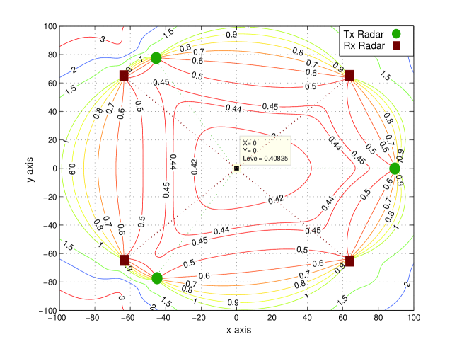
Figure 2: GDOP contours for a symmetric positioning of radars around the axis origin: case (a) with M=3 transmitting radars in a symmetric constellation with the receiving radars set organized in a symmetric constellation of N=4.

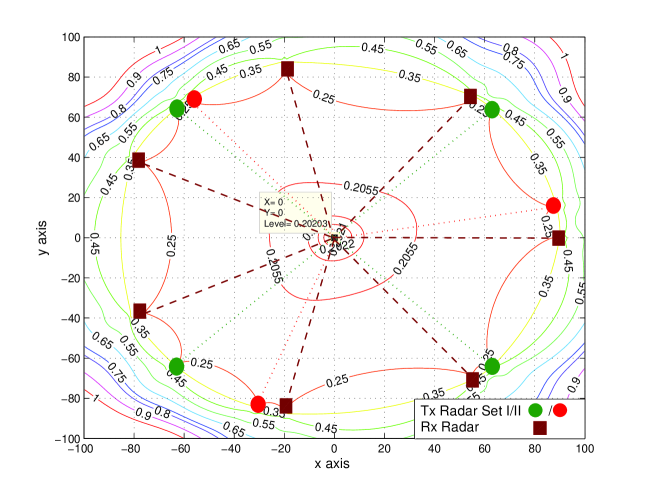
Figure 3: GDOP contours for a symmetric positioning of radars around the axis origin: case (b) with M=7 transmitting radars in two symmetric constellations, one of 3 radars (in red) and second of 4 radars (in green). The receiving radars set are organized in a symmetric constellation of N=7.

Figure 2 and 3 present contour plots of the GDOP values for $3\times 4$ and $7\times 7$ MIMO radar systems, respectively. The sensors are positioned symmetrically around the origin. In Figure 2, the transmitting sensors are located at bearings $\mathbf{\phi}=\left[\phi_{i}=\frac{2\pi\left(i-1\right)}{3},\ i=1,...,3\right],$ and the receiving sensors are positioned at bearings $\mathbf{\varphi}=\left[\varphi_{i}=\frac{\pi}{4}+\frac{2\pi\left(i-1\right)}{4},\ i=1,...,4\right]$. In Figure 3, the $M=7$ transmitting sensors are positioned as a superposition of two symmetrical constellations: the first set includes three radars and the second four. The sets are located at bearings $\mathbf{\phi}=\left[\phi_{i}=\frac{\pi}{18}+\frac{2\pi\left(i-1\right)}{3},\ i=1,...,3;\right.$ $\ \left.\phi_{i}=\frac{\pi}{4}+\frac{2\pi\left(i-1\right)}{4},\ \ i=4,...,7\right]$. The receiving radars, for this case, are set in a single symmetrical constellation with bearings $\mathbf{\varphi}=\left[\varphi_{i}=\frac{2\pi\left(i-1\right)}{7},\ i=1,...,7\right]$. The first noticeable factor in the comparison of the two plots is the higher accuracy obtained with seven radars compared to four radars. For example, the lowest GDOP value in Figure 2, for the $3\times 4$ system is $0.4082,$ while with seven radars (see Figure 3), the lowest GDOP is $0.2020,$ corresponding to a $50\%$ reduction. When a target is located inside the virtual $\left(N+M\right)$-sided system footprint, a higher localization accuracy is obtained than when a target is outside the footprint of the system. In particular, the best localization is obtained for a target at the center of the system. The increase in GDOP values from the center to the footprint boundaries is slow. Outside the footprint, the GDOP values increase rather rapidly.

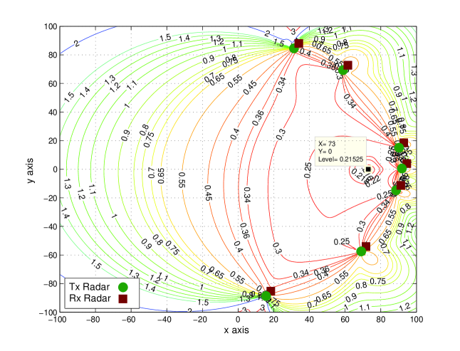
Figure 4: GDOP contours for an asymmetric constellation of the radar set with M=7 transmitting radars and N=7 receiving radars.

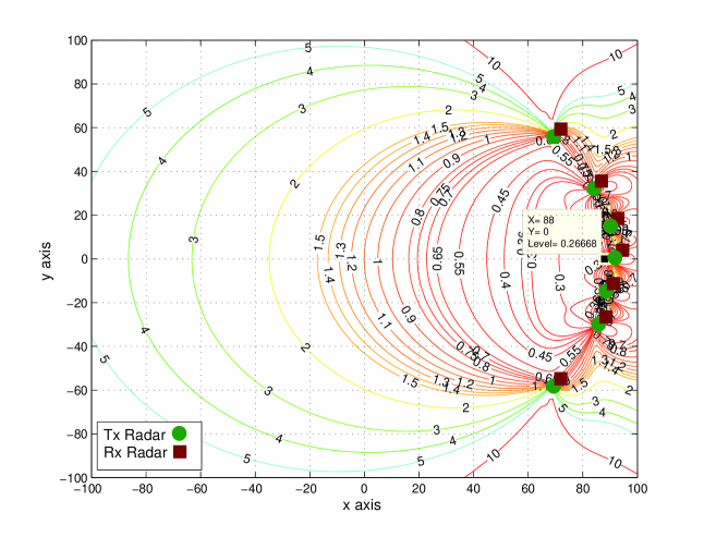
Figure 5: GDOP contours for an asymmetric constellation of the radar set with M=7 transmitting radars and N=7 receiving radars, in the case where the radar are almost aligned.

In Figure 4 and Figure 5, contours of seven non-symmetrically positioned radars are drawn. When the radars are relatively widely spread, as in Figure 4, there are still some areas with good measurement accuracy, though the coverage is shrunk compared to the case with symmetrical deployment of sensors in Figure 3. When the viewing angle of the target is very restricted, as in Figure 5, there is a marked degradation of GDOP values.

These examples demonstrate the main theoretical result of Section IV, namely that a symmetrical deployment of sensors around the target yields the lowest GDOP values. Furthermore, calculating the lowest attainable GDOP value using the optimal results in (72) for a $M\times N$ MIMO radar, we obtain a GDOP value of $\sqrt{2/MN}$, and for $M=N$ it is equal to $\sqrt{2/N^{2}}$. As a numerical example, the lowest GDOPs in Figures 2 and 3 are $\sqrt{2/3\cdot 4}\simeq 0.4082$ and $\sqrt{2/7^{2}}\simeq 0.2020,\$respectively. Comparing this with the results obtained in [29] for the case of passive GPS based systems, with $N$ satellites optimally positioned around the target, for which the lowest achievable GDOP value is $2/\sqrt{N}$, the MIMO system advantage is clearly manifested.

VI Conclusions

In this paper, we have developed analytical expressions for the estimation errors of coherent and non-coherent MIMO radar using the CRLB. It was shown that when the processing is coherent and the phase is processed, there is a reduction in the CRLB values (standard deviation of the estimates) by a factor of $f_{c}/\beta$ over the case when the observations are non-coherent. We referred to this gain as coherency gain. Expressions for the CRLB capture also the impact of the sensors geometry. Further minimization of the localization error reveals a MIMO radar gain directly proportional to the product of the number of transmitting and receiving radars. The smallest CRLB is achieved when the transmitting and receiving sensors are arrayed symmetrically around the target or any a superposition of such sets. The GDOP metric and mapping were introduced as a general tool for the analysis of the localization accuracy with respect to the given radars and target locations. These plots could serve as a tool for choosing favorable radar locations to cover a given target area. While localization by coherent MIMO radar provides significantly better performance than non-coherent processing, it faces the challenge of multisite systems phase synchronizing, and needs to deal with the ambiguities stemming from the large separation between sensors.

Appendix A Derivation of the FIM in (22)

In this appendix, we develop the FIM for the unknown parameter vector $\mathbf{\psi}_{nc}$, based on the conditional pdf in (21). The expression for $\mathbf{J}\left(\mathbf{\psi}\right)=E\left[\nabla_{\mathbf{\psi}}\log p\left(\mathbf{r}|\mathbf{\psi}\right)\left(\nabla_{\mathbf{\psi}}\log p\left(\mathbf{r}|\mathbf{\psi}\right)\right)^{H}\right]=-E\left[\frac{\partial^{2}\log p\left(\mathbf{r}|\mathbf{\psi}\right)}{\partial^{2}\mathbf{\psi}}\right]$ is derived using:

$$\begin{array}[c]{l}\left[\mathbf{J}\left(\mathbf{\psi}_{nc}\right)\right]_{ii^{\prime}}=-E\left[\frac{\partial^{2}\log p\left(\mathbf{r}|\mathbf{\psi}_{nc}\right)}{\partial\tau_{\ell k}\partial\tau_{\ell^{\prime}k^{\prime}}}\right],\\ \left[\mathbf{J}\left(\mathbf{\psi}_{nc}\right)\right]_{(MN+i),(MN+i^{\prime})}=-E\left[\frac{\partial^{2}\log p\left(\mathbf{r}|\mathbf{\psi}_{nc}\right)}{\partial\alpha_{\ell k}^{R}\ \partial\alpha_{\ell^{\prime}k^{\prime}}^{R}}\right],\\ \left[\mathbf{J}\left(\mathbf{\psi}_{nc}\right)\right]_{(2MN+i),(2MN+i^{\prime})}=-E\left[\frac{\partial^{2}\log p\left(\mathbf{r}|\mathbf{\psi}_{nc}\right)}{\partial\alpha_{\ell k}^{I}\ \partial\alpha_{\ell^{\prime}k^{\prime}}^{I}}\right],\\ \left[\mathbf{J}\left(\mathbf{\psi}_{nc}\right)\right]_{(MN+i),(2MN+i^{\prime})}=\left[\mathbf{J}\left(\mathbf{\psi}_{nc}\right)\right]_{(2MN+i),(MN+i^{\prime})}=-E\left[\frac{\partial^{2}\log p\left(\mathbf{r}|\mathbf{\psi}_{nc}\right)}{\partial\alpha_{\ell k}^{R}\ \partial\alpha_{\ell^{\prime}k^{\prime}}^{I}}\right],\\ \left[\mathbf{J}\left(\mathbf{\psi}_{nc}\right)\right]_{i,\left(MN+i^{\prime}\right)}=\left[\mathbf{J}\left(\mathbf{\psi}_{nc}\right)\right]_{\left(MN+i\right),i^{\prime}}=-E\left[\frac{\partial^{2}\log p\left(\mathbf{r}|\mathbf{\psi}_{nc}\right)}{\partial\tau_{\ell k}\ \partial\alpha_{\ell k}^{R}}\right],\\ \left[\mathbf{J}\left(\mathbf{\psi}_{nc}\right)\right]_{i,\left(2MN+i^{\prime}\right)}=\left[\mathbf{J}\left(\mathbf{\psi}_{nc}\right)\right]_{\left(2MN+i\right),i^{\prime}}=-E\left[\frac{\partial^{2}\log p\left(\mathbf{r}|\mathbf{\psi}_{nc}\right)}{\partial\tau_{\ell k}\ \partial\alpha_{\ell k}^{I}}\right],\end{array}$$ (105)

$$\begin{array}[c]{cc}i=(\ell-1)\ast M+k,&i^{\prime}=(\ell^{\prime}-1)\ast M+k^{\prime},\\ \ell,\ell^{\prime}=1,..,N;&k,k^{\prime}=1,..,M;\end{array}\text{ \ \ }$$ (108)

The first derivative of $p\left(\mathbf{r}|\mathbf{\psi}_{nc}\right)$ with respect to the elements of $\mathbf{\tau}$ is:

$$\frac{\partial\left[\log p\left(\mathbf{r}|\mathbf{\psi}_{nc}\right)\right]}{\partial\tau_{\ell k}}= \text{$\frac{1}{\sigma_{w}^{2}}$}{\textstyle\int}\left\{\left[{\small r}_{\ell}{\small(t)-}\overset{M}{\underset{k^{\prime}=1}{\sum}}\alpha_{\ell k^{\prime}}{\small s}_{k^{\prime}}\left(t-\tau_{\ell k^{\prime}}\right)\right]\cdot\alpha_{\ell k}^{\ast}\frac{{\small\partial}\left[{\small s}_{k}^{\ast}\left(t-\tau_{\ell k}\right)\right]}{{\small\partial\tau}_{\ell k}}\right.$$ (109)

$$\left.+\left[{\small r}_{\ell}{\small(t)-}\overset{M}{\underset{k^{\prime}=1}{\sum}}\alpha_{\ell k^{\prime}}{\small s}_{k^{\prime}}\left(t-\tau_{\ell k^{\prime}}\right)\right]^{\ast}\cdot\alpha_{\ell k}\frac{{\small\partial}\left[{\small s}_{k}\left(t-\tau_{\ell k}\right)\right]}{{\small\partial\tau}_{\ell k}}\right\}dt.$$

Applying the second derivative to (109), define a matrix $\mathbf{S}_{nc}$ with the following elements:

$$[\mathbf{S}_{nc}]_{ii^{\prime}} =\frac{\sigma_{w}^{2}}{2}[{\small\mathbf{J}\left(\mathbf{\psi}\right)}]_{ii^{\prime}}=$$ (110)

$$=E\left\{\frac{\partial^{2}}{\partial{\tau_{\ell k}}\partial{\tau_{\ell^{\prime}k^{\prime}}}}\int\left[\alpha_{\ell k}{\small s}_{k}\left(t-{\tau_{\ell k}}\right)\alpha_{\ell k^{\prime}}^{\ast}{\small s}_{k^{\prime}}^{\ast}\left(t-{\tau_{\ell k^{\prime}}}\right)\right.\right.$$

$$\left.+\left.\alpha_{\ell k}^{\ast}{\small s}_{k}^{\ast}\left(t-{\tau_{\ell k}}\right)\alpha_{\ell k^{\prime}}{\small s}_{k^{\prime}}\left(t-{\tau_{\ell k^{\prime}}}\right)\right]dt\right\}$$

$$=\operatorname{Re}\left\{\alpha_{\ell k}\alpha_{\ell^{\prime}k^{\prime}}^{\ast}\left[\frac{\partial^{2}}{\partial{\tau_{\ell k}}\partial{\tau_{\ell^{\prime}k^{\prime}}}}\int{\small s}_{k}\left(t-{\tau_{\ell k}}\right){\small s}_{k^{\prime}}^{\ast}\left(t-{\tau_{\ell k^{\prime}}}\right)dt\right]\right\}.$$

Using matrix notation for compactness,

$$\mathbf{S}_{nc}=\frac{\partial^{2}}{\partial\mathbf{\tau}^{2}}\operatorname{Re}\left[\operatorname*{diag}(\mathbf{\alpha})\mathbf{R}_{s}\operatorname*{diag}\left(\mathbf{\alpha}^{\ast}\right)\right],$$ (111)

where $\operatorname*{diag}(\cdot)$ denotes a diagonal matrix, $\mathbf{\alpha}$ was defined in (11), and we abuse the notation and let

$$\left[\frac{\partial^{2}}{\partial\mathbf{\tau}^{2}}\mathbf{R}_{s}\right]_{ii^{\prime}}\equiv\frac{\partial}{\partial{\tau_{\ell k}}\partial{\tau_{\ell^{\prime}k^{\prime}}}}\left[\mathbf{R}_{s}\right]_{ii^{\prime}}.$$ (112)

The elements of matrix $\mathbf{R}_{s}$ are defined as:

$$\left[\mathbf{R}_{s}\right]_{ii^{\prime}}\equiv\left\{\begin{array}[c]{cc}\int{\small s}_{k}\left(t-{\tau_{\ell k}}\right){\small s}_{k^{\prime}}^{\ast}\left(t-{\tau_{\ell k^{\prime}}}\right)dt&\ell=\ell^{\prime}\\ 0&\ell\neq\ell^{\prime}\end{array}\right..$$ (113)

The second and third terms in (105) define a matrix $\mathbf{\Lambda}_{\alpha}$ with the following elements:

$$[\mathbf{\Lambda}_{\alpha}]_{ii^{\prime}} =[\mathbf{\Lambda}_{\alpha}]_{\left(MN+i\right),\left(MN+i^{\prime}\right)}=\frac{\sigma_{w}^{2}}{2}\left[\mathbf{J}\left(\mathbf{\psi}_{nc}\right)\right]_{(MN+i),(MN+i^{\prime})}=\frac{\sigma_{w}^{2}}{2}\left[\mathbf{J}\left(\mathbf{\psi}_{nc}\right)\right]_{(2MN+i),(2MN+i^{\prime})}$$ (114)

$$=E\left\{\frac{\partial}{\partial\alpha_{\ell^{\prime}k^{\prime}}^{R}}\int\left[\overset{M}{\underset{k^{\prime}=1}{\sum}}{\small s}_{k}\left(t-{\tau_{\ell k}}\right)\alpha_{\ell k^{\prime}}^{\ast}{\small s}_{k^{\prime}}^{\ast}\left(t-{\tau_{\ell k^{\prime}}}\right)\right.\right.$$

$$\left.\left.+\overset{M}{\underset{k^{\prime}=1}{\sum}}{\small s}_{k}^{\ast}\left(t-{\tau_{\ell k}}\right)\alpha_{\ell k^{\prime}}{\small s}_{k^{\prime}}\left(t-{\tau_{\ell k^{\prime}}}\right)\right]dt\right\}$$

$$=\operatorname{Re}\left\{\left[\mathbf{R}_{s}\right]_{ii^{\prime}}\right\},$$

and

$$[\mathbf{\Lambda}_{\alpha}]_{i,\left(MN+i^{\prime}\right)} =[\mathbf{\Lambda}_{\alpha}]_{\left(MN+i\right),i^{\prime}}=\frac{\sigma_{w}^{2}}{2}\left[\mathbf{J}\left(\mathbf{\psi}_{nc}\right)\right]_{(MN+i),(2MN+i^{\prime})}=\frac{\sigma_{w}^{2}}{2}\left[\mathbf{J}\left(\mathbf{\psi}_{nc}\right)\right]_{(2MN+i),(MN+i^{\prime})}$$ (115)

$$=E\left\{\frac{\partial}{\partial\alpha_{\ell^{\prime}k^{\prime}}^{I}}\int\left[\overset{M}{\underset{k^{\prime}=1}{\sum}}\left(j\right){\small s}_{k}\left(t-{\tau_{\ell k}}\right)\alpha_{\ell k^{\prime}}^{\ast}{\small s}_{k^{\prime}}^{\ast}\left(t-{\tau_{\ell k^{\prime}}}\right)\right.\right.$$

$$\left.\left.+\overset{M}{\underset{k^{\prime}=1}{\sum}}\left(-j\right){\small s}_{k}^{\ast}\left(t-{\tau_{\ell k}}\right)\alpha_{\ell k^{\prime}}{\small s}_{k^{\prime}}\left(t-{\tau_{\ell k^{\prime}}}\right)\right]dt\right\}$$

$$=-\operatorname{Im}\left\{\left[\mathbf{R}_{s}\right]_{ii^{\prime}}\right\}.$$

In matrix notation,

$$\mathbf{\Lambda}_{\alpha}=\left[\begin{array}[c]{cc}\operatorname{Re}\left[\mathbf{R}_{s}\right]&-\operatorname{Im}\left[\mathbf{R}_{s}\right]\\ -\operatorname{Im}\left[\mathbf{R}_{s}\right]&\operatorname{Re}\left[\mathbf{R}_{s}\right]\end{array}\right].$$ (116)

The fourth and fifth terms in (105) define the matrix $\mathbf{V}_{nc}$ with the following elements:

$$[\mathbf{V}_{nc}]_{ii^{\prime}} =\frac{\sigma_{w}^{2}}{2}\left[\mathbf{J}\left(\mathbf{\psi}_{nc}\right)\right]_{(MN+i),i^{\prime}}=\frac{\sigma_{w}^{2}}{2}\left[\mathbf{J}\left(\mathbf{\psi}_{nc}\right)\right]_{i,(MN+i^{\prime})}$$ (117)

$$=E\left\{\frac{{\small\partial}}{{\small\partial\tau}_{\ell k}}\frac{\partial}{\partial\alpha^{R}{{}_{\ell^{\prime}k^{\prime}}}}\int\left[\alpha_{\ell k}{\small s}_{k}\left(t-\tau_{\ell k}\right)\alpha_{\ell k^{\prime}}^{\ast}{\small s}_{k^{\prime}}^{\ast}\left(t-\tau_{\ell k^{\prime}}\right)\right.\right.$$

$$\left.\left.+\alpha_{\ell k}^{\ast}{\small s}_{k}^{\ast}\left(t-\tau_{\ell k}\right)\alpha_{\ell k^{\prime}}{\small s}_{k^{\prime}}\left(t-\tau_{\ell k^{\prime}}\right)\right]dt\right\}$$

$$=\operatorname{Re}\left\{\alpha_{\ell k}\frac{{\small\partial}}{{\small\partial\tau}_{\ell k}}\left[\mathbf{R}_{s}\right]_{ii^{\prime}}\right\},$$

and

$$[\mathbf{V}_{nc}]_{i,\left(MN+i^{\prime}\right)} =\frac{\sigma_{w}^{2}}{2}\left[\mathbf{J}\left(\mathbf{\psi}_{nc}\right)\right]_{(2MN+i),i^{\prime}}=\frac{\sigma_{w}^{2}}{2}\left[\mathbf{J}\left(\mathbf{\psi}_{nc}\right)\right]_{i,(2MN+i^{\prime})}$$ (118)

$$=E\left\{\frac{{\small\partial}}{{\small\partial\tau}_{\ell k}}\frac{\partial}{\partial\alpha^{I}{{}_{\ell^{\prime}k^{\prime}}}}\int\left[\alpha_{\ell k}{\small s}_{k}\left(t-\tau_{\ell k}\right)\alpha_{\ell k^{\prime}}^{\ast}{\small s}_{k^{\prime}}^{\ast}\left(t-\tau_{\ell k^{\prime}}\right)\right.\right.$$

$$\left.\left.+\alpha_{\ell k}^{\ast}{\small s}_{k}^{\ast}\left(t-\tau_{\ell k}\right)\alpha_{\ell k^{\prime}}{\small s}_{k^{\prime}}\left(t-\tau_{\ell k^{\prime}}\right)\right]dt\right\}$$

$$=-\operatorname{Im}\left\{\alpha_{\ell k}\frac{{\small\partial}}{{\small\partial\tau}_{\ell k}}\left[\mathbf{R}_{s}\right]_{ii^{\prime}}\right\}.$$

In matrix notation:

$$\mathbf{V}_{nc}=\left[\begin{array}[c]{cc}\frac{\partial}{\partial\mathbf{\tau}}\operatorname{Re}\left[\operatorname*{diag}(\mathbf{\alpha})\mathbf{R}_{s}\right];&-\frac{\partial}{\partial\mathbf{\tau}}\operatorname{Im}\left[\operatorname*{diag}(\mathbf{\alpha})\mathbf{R}_{s}\right]\end{array}\right].$$ (119)

Orthogonal Waveforms

Orthogonality implies that all cross elements $\int{\small s}_{k}\left(t-\tau_{\ell k}\right){\small s}_{k^{\prime}}^{\ast}\left(t-\tau_{\ell^{\prime}k^{\prime}}\right)dt=0,$ for $\ell\neq\ell^{\prime}$ and $k\neq k^{\prime},$and after some algebra, the matrices defined by (110)-(118) take the following form:

$$\begin{array}[c]{c}\left[\mathbf{S}_{nc}\right]_{ii^{\prime}}=\left\{\begin{array}[c]{cc}4\pi^{2}\beta^{2}\left[\left|\alpha_{lk}\right|^{2}\beta_{R_{k}}^{2}\right]&i=i^{\prime}\\ 0&i\neq i^{\prime}\end{array}\right.\\ [\mathbf{\Lambda}_{\alpha}]_{ii^{\prime}}=[\mathbf{\Lambda}_{\alpha}]_{\left(MN+i\right),\left(MN+i^{\prime}\right)}=\left\{\begin{array}[c]{cc}1&i=i^{\prime}\\ 0&i\neq i^{\prime}\end{array}\right.\\ [\mathbf{\Lambda}_{\alpha}]_{i,\left(MN+i^{\prime}\right)}=[\mathbf{\Lambda}_{\alpha}]_{\left(MN+i\right),i^{\prime}}=0\\ [\mathbf{V}_{nc}]_{ii^{\prime}}=0\\ [\mathbf{V}_{nc}]_{i,\left(MN+i^{\prime}\right)}=0.\end{array}$$ (120)

Appendix B Derivation of the FIM in (34)

In this appendix, we develop the FIM for the unknown parameter vector $\mathbf{\psi}_{c}$, based on the conditional pdf in (43). The expression for $\mathbf{J}\left(\mathbf{\psi}\right)=E\left\{\nabla_{\mathbf{\psi}}\log p\left(\mathbf{r}|\mathbf{\psi}\right)\left(\nabla_{\mathbf{\psi}}\log p\left(\mathbf{r}|\mathbf{\psi}\right)\right)^{H}\right\}=-E\left[\frac{\partial^{2}\log p\left(\mathbf{r}|\mathbf{\psi}\right)}{\partial^{2}\mathbf{\psi}}\right]$ is derived using:

$$\begin{array}[c]{l}\left[\mathbf{J}\left(\mathbf{\psi}_{c}\right)\right]_{ii^{\prime}}=-E\left[\frac{\partial^{2}\log p\left(\mathbf{r}|\mathbf{\psi}_{c}\right)}{\partial\tau_{\ell k}\partial\tau_{\ell^{\prime}k^{\prime}}}\right],\\ \left[\mathbf{J}\left(\mathbf{\psi}_{c}\right)\right]_{(MN+1),(MN+1)}=-E\left[\frac{\partial^{2}\log p\left(\mathbf{r}|\mathbf{\psi}_{c}\right)}{\left(\partial\zeta^{R}\right)^{2}\ }\right],\\ \left[\mathbf{J}\left(\mathbf{\psi}_{c}\right)\right]_{(MN+2),(MN+2)}=-E\left[\frac{\partial^{2}\log p\left(\mathbf{r}|\mathbf{\psi}_{c}\right)}{\left(\partial\zeta^{I}\right)^{2}}\right],\\ \left[\mathbf{J}\left(\mathbf{\psi}_{c}\right)\right]_{(MN+1),(MN+2)}=\left[\mathbf{J}\left(\mathbf{\psi}_{c}\right)\right]_{(MN+2),(MN+1)}=-E\left[\frac{\partial^{2}\log p\left(\mathbf{r}|\mathbf{\psi}_{c}\right)}{\partial\zeta^{R}\ \partial\zeta^{I}}\right],\\ \left[\mathbf{J}\left(\mathbf{\psi}_{c}\right)\right]_{i,\left(MN+1\right)}=\left[\mathbf{J}\left(\mathbf{\psi}_{c}\right)\right]_{\left(MN+1\right),i^{\prime}}=-E\left[\frac{\partial^{2}\log p\left(\mathbf{r}|\mathbf{\psi}_{c}\right)}{\partial\tau_{\ell k}\ \partial\zeta^{R}\ }\right],\\ \left[\mathbf{J}\left(\mathbf{\psi}_{c}\right)\right]_{i,\left(MN+2\right)}=\left[\mathbf{J}\left(\mathbf{\psi}_{c}\right)\right]_{\left(MN+2\right),i^{\prime}}=-E\left[\frac{\partial^{2}\log p\left(\mathbf{r}|\mathbf{\psi}_{c}\right)}{\partial\tau_{\ell k}\ \partial\zeta^{I}}\right],\end{array}$$ (127)

$$\begin{array}[c]{cc}i=(\ell-1)\ast M+k,&i^{\prime}=(\ell^{\prime}-1)\ast M+k^{\prime},\\ \ell,\ell^{\prime}=1,..,N;&k,k^{\prime}=1,..,M.\end{array}\text{ \ .\ }$$ (130)

The first derivative of $p\left(\mathbf{r}|\mathbf{\psi}_{c}\right)$ with respect to the elements of $\mathbf{\tau}$ is:

$$\frac{\partial\left[\log p\left(\mathbf{r}|\mathbf{\psi}_{c}\right)\right]}{\partial\tau_{\ell k}}= \text{$\frac{1}{\sigma_{w}^{2}}$}{\textstyle\int}\left\{\left[{\small r}_{\ell}{\small(t)-}\overset{M}{\underset{k^{\prime}=1}{\sum}}\zeta\exp\left(-j2\pi f_{c}\tau_{\ell k^{\prime}}\right){\small s}_{k^{\prime}}\left(t-\tau_{\ell k^{\prime}}\right)\right]\cdot\zeta^{\ast}\frac{{\small\partial}\left[\exp\left(j2\pi f_{c}\tau_{\ell k}\right){\small s}_{k}^{\ast}\left(t-\tau_{\ell k}\right)\right]}{{\small\partial\tau}_{\ell k}}\right.$$ (131)

$$\left.+\left[{\small r}_{\ell}{\small(t)-}\overset{M}{\underset{k^{\prime}=1}{\sum}}\zeta\exp\left(-j2\pi f_{c}\tau_{\ell k^{\prime}}\right){\small s}_{k^{\prime}}\left(t-\tau_{\ell k^{\prime}}\right)\right]^{\ast}\cdot\zeta\frac{{\small\partial}\left[\exp\left(-j2\pi f_{c}\tau_{\ell k}\right){\small s}_{k}\left(t-\tau_{\ell k}\right)\right]}{{\small\partial\tau}_{\ell k}}\right\}dt.$$

Applying the second derivative to (131) define a matrix $\mathbf{S}_{nc}$ with the following elements:

$$[\mathbf{S}_{c}]_{ii^{\prime}} =\frac{\sigma_{w}^{2}}{2}[{\small\mathbf{J}\left(\mathbf{\psi}\right)}]_{ii^{\prime}}=$$ (132)

$$=E\left\{\frac{\partial^{2}}{\partial{\tau_{\ell k}}\partial{\tau_{\ell^{\prime}k^{\prime}}}}\int\left[\zeta\zeta^{\ast}\exp\left(j2\pi f_{c}\left(\tau_{\ell k}-\tau_{\ell^{\prime}k^{\prime}}\right)\right){\small s}_{k^{\prime}}\left(t-{\tau_{\ell k^{\prime}}}\right){\small s}_{k}^{\ast}\left(t-{\tau_{\ell k}}\right)\right.\right.$$

$$\left.+\left.\zeta^{\ast}\zeta\exp\left(-j2\pi\left(\tau_{\ell k}-\tau_{\ell k^{\prime}}\right)\right){\small s}_{k^{\prime}}^{\ast}\left(t-{\tau_{\ell k^{\prime}}}\right){\small s}_{k}\left(t-{\tau_{\ell k}}\right)\right]dt\right\}$$

$$=\operatorname{Re}\left\{\left|\zeta\right|^{2}\left[\frac{\partial^{2}}{\partial{\tau_{\ell k}}\partial{\tau_{\ell^{\prime}k^{\prime}}}}\left(\exp\left(-j2\pi f_{c}\left(\tau_{\ell k}-\tau_{\ell^{\prime}k^{\prime}}\right)\right)\left[\mathbf{R}_{s}\right]_{ii^{\prime}}\right)\right]\right\}.$$

In matrix form,

$$\mathbf{S}_{c}=\left|\zeta\right|^{2}\frac{\partial^{2}}{\partial\mathbf{\tau}^{2}}\operatorname{Re}\left\{\operatorname*{diag}(\mathbf{e)R}_{s}\operatorname*{diag}\left(\mathbf{e}^{{}^{\ast}}\right)\right\},$$ (133)

where the operator $\frac{\partial^{2}}{\partial\mathbf{\tau}^{2}}$ and the matrix $\mathbf{\mathbf{R}_{s}}$ were defined in Appendix A, $\mathbf{e}=\left[\exp\left(-2\pi f_{c}\tau_{11}\right),\exp\left(-2\pi f_{c}\tau_{12}\right),\right.$ $\left....,\exp\left(-2\pi f_{c}\tau_{MN}\right)\right]$.

The second and third terms in (127) define a matrix $\mathbf{\Lambda}_{\alpha c}$ with the following elements:

$$[\mathbf{\Lambda}_{\alpha c}]_{11} =[\mathbf{\Lambda}_{\alpha c}]_{22}=\frac{\sigma_{w}^{2}}{2}\left[\mathbf{J}\left(\mathbf{\psi}_{c}\right)\right]_{(MN+1),(MN+1)}=\frac{\sigma_{w}^{2}}{2}\left[\mathbf{J}\left(\mathbf{\psi}_{c}\right)\right]_{(MN+2),(MN+2)}$$ (134)

$$=E\left\{\overset{N}{\underset{\ell=1}{\sum}}\overset{M}{\underset{k=1}{\sum}}\int\left[\overset{M}{\underset{k^{\prime}=1}{\sum}}\exp\left(-j2\pi f_{c}\left(\tau_{\ell k}-\tau_{\ell k^{\prime}}\right)\right){\small s}_{k}\left(t-{\tau_{\ell k}}\right){\small s}_{k^{\prime}}^{\ast}\left(t-{\tau_{\ell k^{\prime}}}\right)\right.\right.$$

$$\left.\left.+\overset{M}{\underset{k^{\prime}=1}{\sum}}\exp\left(j2\pi f_{c}\left(\tau_{\ell k}-\tau_{\ell k^{\prime}}\right)\right){\small s}_{k}^{\ast}\left(t-{\tau_{\ell k}}\right){\small s}_{k^{\prime}}\left(t-{\tau_{\ell k^{\prime}}}\right)\right]dt\right\}$$

$$=\operatorname{Re}\left\{\overset{N}{\underset{\ell=1}{\sum}}\overset{N}{\underset{\ell^{\prime}=1}{\sum}}\overset{M}{\underset{k=1}{\sum}}\overset{M}{\underset{k^{\prime}=1}{\sum}}\exp\left(-j2\pi f_{c}\left(\tau_{\ell k}-\tau_{\ell^{\prime}k^{\prime}}\right)\right)\left[\mathbf{R}_{s}\right]_{ii^{\prime}}\right\},$$

and

$$[\mathbf{\Lambda}_{\alpha c}]_{12} =[\mathbf{\Lambda}_{\alpha c}]_{21}=\frac{\sigma_{w}^{2}}{2}\left[\mathbf{J}\left(\mathbf{\psi}_{c}\right)\right]_{(MN+1)(MN+2)}=\frac{\sigma_{w}^{2}}{2}\left[\mathbf{J}\left(\mathbf{\psi}_{c}\right)\right]_{(MN+2)(MN+1)}=$$ (135)

$$=E\left\{\overset{N}{\underset{\ell=1}{\sum}}\overset{M}{\underset{k=1}{\sum}}\int\left[\overset{M}{\underset{k^{\prime}=1}{\sum}}\left(j\right)^{\ast}\exp\left(-j2\pi f_{c}\left(\tau_{\ell k}-\tau_{\ell k^{\prime}}\right)\right){\small s}_{k}\left(t-{\tau_{\ell k}}\right){\small s}_{k^{\prime}}^{\ast}\left(t-{\tau_{\ell k^{\prime}}}\right)\right.\right.$$

$$\left.\left.+\overset{M}{\underset{k^{\prime}=1}{\sum}}\left(j\right)\exp\left(j2\pi f_{c}\left(\tau_{\ell k}-\tau_{\ell k^{\prime}}\right)\right){\small s}_{k}^{\ast}\left(t-{\tau_{\ell k}}\right){\small s}_{k^{\prime}}\left(t-{\tau_{\ell k^{\prime}}}\right)\right]dt\right\}$$

$$=-\operatorname{Im}\left\{\overset{N}{\underset{\ell=1}{\sum}}\overset{N}{\underset{\ell^{\prime}=1}{\sum}}\overset{M}{\underset{k=1}{\sum}}\overset{M}{\underset{k^{\prime}=1}{\sum}}\exp\left(-j2\pi f_{c}\left(\tau_{\ell k}-\tau_{\ell^{\prime}k^{\prime}}\right)\right)\left[\mathbf{R}_{s}\right]_{ii^{\prime}}\right\}.$$

In matrix form,

$$\mathbf{\Lambda}_{\alpha c}=\left[\begin{array}[c]{cc}\operatorname{Re}\left[\mathbf{eR}_{s}\mathbf{e}^{H}\right]&-\operatorname{Im}\left[\mathbf{eR}_{s}\mathbf{e}^{H}\right]\\ -\operatorname{Im}\left[\mathbf{eR}_{s}\mathbf{e}^{H}\right]&\operatorname{Re}\left[\mathbf{eR}_{s}\mathbf{e}^{H}\right]\end{array}\right].$$ (136)

The fourth and fifth terms in (127) define the matrix $\mathbf{V}_{c}$ with the following elements:

$$[\mathbf{V}_{c}]_{i1} =\frac{\sigma_{w}^{2}}{2}\left[\mathbf{J}\left(\mathbf{\psi}_{c}\right)\right]_{i,(MN+1)}=\frac{\sigma_{w}^{2}}{2}\left[\mathbf{J}\left(\mathbf{\psi}_{c}\right)\right]_{(MN+1),i^{\prime}}$$ (137)

$$=E\left\{\frac{\partial}{\partial{\tau_{\ell k}}}\int\left[\zeta\overset{M}{\underset{k^{\prime}=1}{\sum}}\exp\left(-j2\pi f_{c}\left(\tau_{\ell k}-\tau_{\ell k^{\prime}}\right)\right){\small s}_{k}\left(t-\tau_{\ell k}\right){\small s}_{k^{\prime}}^{\ast}\left(t-\tau_{\ell k^{\prime}}\right)\right.\right.$$

$$\left.\left.+\zeta^{\ast}\overset{M}{\underset{k^{\prime}=1}{\sum}}\exp\left(j2\pi f_{c}\left(\tau_{\ell k}-\tau_{\ell k^{\prime}}\right)\right){\small s}_{k}^{\ast}\left(t-\tau_{\ell k}\right){\small s}_{k^{\prime}}\left(t-\tau_{\ell k^{\prime}}\right)\right]dt\right\}$$

$$=\frac{{\small\partial}}{{\small\partial\tau}_{\ell k}}\operatorname{Re}\left\{\overset{N}{\underset{\ell^{\prime}=1}{\sum}}\overset{M}{\underset{k^{\prime}=1}{\sum}}\zeta\exp\left(-j2\pi f_{c}\left(\tau_{\ell k}-\tau_{\ell^{\prime}k^{\prime}}\right)\right)\left[\mathbf{R}_{s}\right]_{ii^{\prime}}dt\right\},$$

and

$$[\mathbf{V}_{c}]_{i2} =\frac{\sigma_{w}^{2}}{2}\left[\mathbf{J}\left(\mathbf{\psi}_{c}\right)\right]_{i,(MN+2)}=\frac{\sigma_{w}^{2}}{2}\left[\mathbf{J}\left(\mathbf{\psi}_{c}\right)\right]_{(MN+2),i^{\prime}}$$ (138)

$$=E\left\{\frac{\partial}{\partial{\tau_{\ell k}}}\int\left[\left(j\zeta\right)\overset{M}{\underset{k^{\prime}=1}{\sum}}\exp\left(-j2\pi f_{c}\left(\tau_{\ell k}-\tau_{\ell k^{\prime}}\right)\right){\small s}_{k}\left(t-\tau_{\ell k}\right){\small s}_{k^{\prime}}^{\ast}\left(t-\tau_{\ell k^{\prime}}\right)\right.\right.$$

$$\left.\left.+\left(j\zeta\right)^{\ast}\overset{M}{\underset{k^{\prime}=1}{\sum}}\exp\left(j2\pi f_{c}\left(\tau_{\ell k}-\tau_{\ell k^{\prime}}\right)\right){\small s}_{k}^{\ast}\left(t-\tau_{\ell k}\right){\small s}_{k^{\prime}}\left(t-\tau_{\ell k^{\prime}}\right)\right]dt\right\}$$

$$=-\frac{{\small\partial}}{{\small\partial\tau}_{\ell k}}\operatorname{Im}\left\{\overset{N}{\underset{\ell^{\prime}=1}{\sum}}\overset{M}{\underset{k^{\prime}=1}{\sum}}\zeta\exp\left(-j2\pi f_{c}\left(\tau_{\ell k}-\tau_{\ell^{\prime}k^{\prime}}\right)\right)\left[\mathbf{R}_{s}\right]_{ii^{\prime}}dt\right\}.$$

In matrix form,

$$\mathbf{V}_{c}=\left[\begin{array}[c]{cc}\frac{\partial}{\partial\mathbf{\tau}}\operatorname{Re}\left\{\zeta\left[\operatorname*{diag}(\mathbf{e)R}_{s}\right]\mathbf{e}^{H}\right\};&-\frac{\partial}{\partial\mathbf{\tau}}\operatorname{Im}\left\{\zeta\left[\operatorname*{diag}(\mathbf{e)R}_{s}\right]\mathbf{e}^{H}\right\}\end{array}\right].$$ (139)

Orthogonal Waveforms

Orthogonality implies that all cross elements $\int{\small s}_{k}\left(t-\tau_{\ell k}\right){\small s}_{k^{\prime}}^{\ast}\left(t-\tau_{\ell^{\prime}k^{\prime}}\right)dt=o$ for $\ell\neq\ell^{\prime}$ and $k\neq k^{\prime}$. Therefore, the matrices defined by (132)-(138) take the following form:

$$\begin{array}[c]{c}\left[\mathbf{S}_{c_{or}}\right]_{ii^{\prime}}=\left\{\begin{array}[c]{cc}4\pi^{2}\left|\zeta\right|^{2}f_{c}^{2}f_{R_{k}}&i=i^{\prime}\\ 0&i\neq i^{\prime}\end{array}\right.\\ [\mathbf{\Lambda}_{\alpha c_{or}}]_{11}=[\mathbf{\Lambda}_{\alpha_{or}}]_{22}=\left\{\begin{array}[c]{cc}\frac{1}{MN}&i=i^{\prime}\\ 0&i\neq i^{\prime}\end{array}\right.\\ [\mathbf{\Lambda}_{\alpha c_{or}}]_{21}=[\mathbf{\Lambda}_{\alpha_{or}}]_{12}=0\\ [\mathbf{V}_{c_{or}}]_{i1}=2\pi\zeta^{I}f_{c}\\ [\mathbf{V}_{c_{or}}]_{i2}=-2\pi\zeta^{R}f_{c}.\end{array}$$ (140)

where $f_{R_{k}}=\left(1+\frac{\beta_{k}^{2}}{f_{c}^{2}}\right)$. When we invoke the narrowband assumption $\beta_{k}^{2}/f_{c}^{2}\ll 1$ it follows that $f_{R_{k}}\simeq 1$.

Appendix C Computation of (36)

The submatrix $\left[\mathbf{C}_{CRLB_{c}}\right]_{2\times 2}$ is defined as:

$$\left[\mathbf{C}_{CRLB_{c}}\right]_{2\times 2}=\left[\mathbf{J}\left(\mathbf{\theta}_{c}\right)\right]_{2\times 2}^{-1}.$$ (141)

For a given matrix of the form:

$$\mathbf{J}\left(\mathbf{\theta}_{c}\right)=\left[\begin{array}[c]{cc}\mathbf{HS}_{c}\mathbf{H}^{T}&\mathbf{HV}_{c}\\ \mathbf{V}_{c}^{T}\mathbf{H}^{T}&\mathbf{\Lambda}_{{\normalsize\alpha c}}\end{array}\right],$$ (142)

where $\mathbf{\Lambda}_{{\normalsize\alpha c}}$ is a diagonal matrix of the form $\mathbf{\Lambda}_{{\normalsize\alpha c}}=d\mathbf{I}_{2\times 2}$, and $d$ is some constant.

By definition, the value of $\left[\mathbf{J}\left(\mathbf{\theta}_{c}\right)\right]_{1,1}^{-1}$ is obtained by:

$$\left[\mathbf{J}\left(\mathbf{\theta}_{c}\right)\right]_{1,1}^{-1}=\frac{\left|\widetilde{\mathbf{J}}\left(\mathbf{\theta}_{c}\right)_{ex\left(1,1\right)}\right|}{\left|\mathbf{J}\left(\mathbf{\theta}_{c}\right)\right|},$$ (143)

where $\left|\mathbf{\cdot}\right|$ denotes the determinant, and $\widetilde{\mathbf{J}}\left(\mathbf{\theta}\right)_{ex\left(1,1\right)}$ is a submatrix, obtained by removing the first row and the first column of the $\mathbf{J}\left(\mathbf{\theta}_{c}\right)$ matrix. The determinant of $\mathbf{J}\left(\mathbf{\theta}_{c}\right)$, using the property that the determinant of a matrix does not change under linear operations, is:

$$\left|\mathbf{J}\left(\mathbf{\theta}_{c}\right)\right|=\left|\begin{array}[c]{cc}\mathbf{H\mathbf{S}}_{c}\mathbf{H}^{T}-\mathbf{V}_{c}^{T}\mathbf{H}^{T}\mathbf{\Lambda}_{{\normalsize\zeta}}^{-1}\mathbf{HV}_{c}&\mathbf{0}\\ \mathbf{V}_{c}^{T}\mathbf{H}^{T}&\mathbf{\Lambda}_{{\normalsize\alpha c}}\end{array}\right|.$$ (144)

This can be calculated and expressed as:

$$\left|\mathbf{J}\left(\mathbf{\theta}_{c}\right)\right|=\left|\mathbf{H\mathbf{\mathbf{S}}}_{c}\mathbf{H}^{T}-\mathbf{V}_{c}^{T}\mathbf{H}^{T}\mathbf{\Lambda}_{{\normalsize\zeta}}^{-1}\mathbf{HV}\right|\left|\mathbf{\Lambda}_{{\normalsize\alpha c}}\right|.$$ (145)

Repeating the same for the matrix $\widetilde{\mathbf{J}}\left(\mathbf{\theta}_{c}\right)_{ex\left(1,1\right)}$:

$$\widetilde{\mathbf{J}}\left(\mathbf{\theta}_{c}\right)_{ex\left(1,1\right)}=\left[\begin{array}[c]{cc}\widetilde{\mathbf{H\mathbf{\mathbf{S}}}_{c}\mathbf{H}^{T}}_{ex\left(1,1\right)}&\widetilde{\mathbf{HV}_{c}}_{ex\left(1,\right)}\\ \widetilde{\mathbf{V}_{c}^{T}\mathbf{H}^{T}}_{ex\left(,1\right)}&\mathbf{\Lambda}_{{\normalsize\alpha c}}\end{array}\right].$$ (146)

Using the same matrix manipulation, we get:

$$\left|\widetilde{\mathbf{J}}\left(\mathbf{\theta}_{c}\right)_{ex\left(1,1\right)}\right|=\left|\widetilde{\mathbf{H\mathbf{S}}_{c}\mathbf{H}^{T}}-\widetilde{\mathbf{V}_{c}^{T}\mathbf{H}^{T}}\mathbf{\Lambda}_{{\normalsize\alpha c}}^{-1}\widetilde{\mathbf{HV}_{c}}\right|\left|\mathbf{\Lambda}_{{\normalsize\alpha c}}\right|,$$ (147)

and using terms (145) and (147) in (143) yields:

$$\left[\mathbf{J}\left(\mathbf{\theta}_{c}\right)\right]_{1,1}^{-1}=\frac{\left|\widetilde{\mathbf{H\mathbf{S}}_{c}\mathbf{H}^{T}}-\widetilde{\mathbf{V}_{c}^{T}\mathbf{H}^{T}}\mathbf{\Lambda}_{{\normalsize\alpha c}}^{-1}\widetilde{\mathbf{HV}_{c}}\right|}{\left|\mathbf{H\mathbf{S}}_{c}\mathbf{H}^{T}-\mathbf{V}_{c}^{T}\mathbf{H}^{T}\mathbf{\Lambda}_{{\normalsize\alpha c}}^{-1}\mathbf{HV}_{c}\right|}.$$ (148)

By definition, this expression is identical to:

$$\left[\mathbf{J}\left(\mathbf{\theta}_{c}\right)\right]_{1,1}^{-1}{\normalsize=}\left[\left(\mathbf{H\mathbf{S}}_{c}\mathbf{H}^{T}-\mathbf{V}_{c}^{T}\mathbf{H}^{T}\mathbf{\Lambda}_{{\normalsize\alpha c}}^{-1}\mathbf{HV}_{c}\right)^{-1}\right]_{1,1}.$$ (149)

Repeating the process for term located at $\left(1,2\right)$, $\left(2,1\right)$, and $\left(2,2\right)$,  results in:

$$\left[\mathbf{C}_{C{\normalsize RLB}_{c_{or}}}\right]_{2\times 2}{\normalsize=}\left(\mathbf{H\mathbf{S}}_{c}\mathbf{H}^{T}-\mathbf{V}_{c}^{T}\mathbf{H}^{T}\mathbf{\Lambda}_{{\normalsize\alpha c}}^{-1}\mathbf{HV}_{c}\right)^{-1}.$$ (150)

Appendix D Derivation of Covariance of Observation Noise (78)

For a set of received waveforms $r_{\ell}\left(t\right),$ $1\leq\ell\leq N,$ the time delay estimates $\mu=\left[\mu_{11},\mu_{12},...,\mu_{MN}\right]^{T}$ are determined by maximizing the following statistic:

$$\mu_{\ell k}=\arg\max_{v}\left[\exp\left(j2\pi f_{c}v\right)\int_{T}r_{\ell}\left(t\right)s_{k}^{\ast}\left(t-v\right)dt\right].$$ (151)

Equivalently,

$$\frac{d}{dv}\left[\exp\left(j2\pi f_{c}v\right)\int_{T}r_{\ell}\left(t\right)s_{k}^{\ast}\left(t-v\right)dt\right]_{v=\mu_{\ell k}}=0.$$ (152)

The time delay estimates are expressed in (82). The properties of the noise $\epsilon_{\ell k}$ can be computed from (8), and (2). It is not difficult to show that the following relation holds:

$$\left.\frac{dg(v)}{dv}\right|_{v=\mu_{\ell k}}+n_{\ell k}=0,$$ (153)

where

$$g(v)=\zeta\int_{T}\exp\left[j2\pi f_{c}\left(v-\tau_{\ell k}\right)\right]s_{k}\left(t-\tau_{\ell k}\right)s_{k}^{\ast}\left(t-v\right)dt,$$ (154)

and

$$n_{\ell k}=\int_{T}\frac{d}{dv}w_{\ell}(t)s_{k}^{\ast}\left(t-v\right)\exp\left(j2\pi f_{c}v\right)dt.$$ (155)

We wish to write (153) in the form of (82). With a few algebraic manipulations, including expanding $g(v)$ in a Taylor series around $\tau_{\ell k},$ and neglecting terms $o\left[\left(\tau_{\ell k}-\widehat{\tau}_{\ell k}\right)^{3}\right],$ it can be shown that

$$\mu_{\ell k}=\tau_{\ell k}+\frac{n_{\ell k}}{4\pi^{2}f_{c}^{2}\left(1+\frac{\beta_{k}^{2}}{f_{c}^{2}}\right)\zeta}.$$ (156)

Comparing this with (82), and invoking the narrowband assumption $\beta_{k}^{2}/f_{c}^{2}\ll 1$, we have for the error term

$$\epsilon_{\ell k}\simeq\frac{n_{\ell k}}{4\pi^{2}\zeta f_{c}^{2}}.$$ (157)

To find the first and second order statistics of $\epsilon_{\ell k},$ we need the statistical characterization of $n_{\ell k}$. As previously stated, we assume the receiver noise $w_{\ell}(t)$ is a Gaussian random process with zero mean and autocorrelation function $\sigma_{w}^{2}\delta(\tau)$. Since $n_{\ell k}$ is a linear transformation of the process $w_{\ell}(t),$ since the mean $w_{\ell}(t)$ is zero, $E\left[n_{\ell k}\right]=0.$ Similarly, it can be shown that

$$E\left[n_{\ell k}{}n_{nm}^{\ast}\right]=\left\{\begin{array}[c]{lc}0&\forall\ell k\neq nm\\ 2\pi^{2}\sigma_{w}^{2}f_{c}^{2}&\forall\ell k=nm\text{ }\end{array}\right..$$ (158)

Using these results, we finally get

$$E\left[\epsilon_{\ell k}\epsilon_{nm}^{\ast}\right] =\frac{E\left[n_{\ell k}{}n_{nm}\right]}{16\pi^{4}\left|\zeta\right|^{2}f_{c}^{4}}$$ (159)

$$=\left\{\begin{array}[c]{lc}0&\forall\ell k\neq nm\\ \frac{1}{8\pi^{2}f_{c}^{2}\left(\left|\zeta\right|^{2}/\sigma_{w}^{2}\right)}&\forall\ell k=nm\text{ }\end{array}\right.,$$ (162)

concluding that the covariance matrix of the terms $\epsilon_{\ell k}$ is given by:

$$\mathbf{C}_{\mathbf{\epsilon}}=\frac{1}{8\pi^{2}f_{c}^{2}\left|\zeta\right|^{2}/\sigma_{w}^{2}}\mathbf{I}_{MN\times MN}.$$ (163)

References

- [1] A. Haimovich, R. Blum, L. Cimini, , ”MIMO Radar with Widely Separated antennas”, IEEE Signal Proc. Magazine, January 2008.
- [2] Jian Li, and Petre Stoica, ”MIMO Radar with Colocated antennas”, IEEE Signal Proc. Magazine, September 2007, pp. 106–114.
- [3] E. Fishler, A. Haimovich, R. Blum, D. Chizhik, L. Cimini, and R. Valenzuela, “MIMO radar: An idea whose time has come,” in Proc. IEEE Radar Conf., April 2004, pp. 71–78.
- [4] J. Li and P. Stoica, “MIMO radar—diversity means superiority,” in Proc. 14th Annu. Workshop Adaptive Sensor Array Processing, MIT Lincoln Laboratory, Lexington, MA, June 2006.
- [5] E. Fishler, A. Haimovich, R. Blum, L. Cimini, D. Chizhik, and R. Valenzuela, “Performance of MIMO radar systems: Advantages of angular diversity,” in Proc. 38th Asilomar Conf. Signals, Syst. Comput., Pacific Grove, CA, Nov. 2004, vol. 1, pp. 305–309.
- [6] D. W. Bliss and K. W. Forsythe, “Multiple-input multiple-output (MIMO) radar and imaging: degrees of freedom and resolution,” in Proc. of 37th Asilomar Conference on Signals, Systems and Computers, Nov. 2003, pp. 54-59.
- [7] J. Li, P. Stoica, and Y. Xie, “On probing signal design for MIMO radar,” in Proc.40th Asilomar Conf. Signals, Syst. Comput. , Pacific Grove, CA, pp. 31–35, Oct. 2006.
- [8] F. C. Robey, S. Coutts, D. Weikle, J. C. McHarg, and K. Cuomo, “MIMO radar theory and experimental results,” in the 38th Asilomar Conference on Signals, Systems and Computers, November 2004, pp. 300–304.
- [9] J. Tabrikian, “Barankin bounds for target localization by MIMO radars,” in Proc. 4th IEEE Workshop on Sensor Array and Multi-Channel Processing, Waltham, MA, pp. 278–281, July 2006.
- [10] I. Bekkerman and J. Tabrikian, “Target detection and localization using MIMO radars and sonars,” IEEE Trans. on Sig. Proc., vol. 54, Oct. 2006, pp. 3873- 3883.
- [11] J. Li, P. Stoica, L. Xu, and W. Roberts, “On parameter identifiability of MIMO radar,” IEEE Signal Processing Lett., vol. 14, no. 12, Dec. 2007.
- [12] L. Xu, J. Li, and P. Stoica, “Adaptive techniques for MIMO radar,” 14th IEEE Workshop on Sensor Array and Multi-channel Processing, Waltham, MA, July 2006.
- [13] E. Fishler, A. Haimovich, R. Blum, L. Cimini, D. Chizhik, and R. Valenzuela, “Spatial diversity in radars - models and detection performance,” IEEE Trans. on Sig. Proc., vol. 54, March 2006, pp. 823-838.
- [14] K.W. Forsythe and D.W. Bliss, “Waveform correlation and optimization issues for MIMO radar,” in Proc. 39th Asilomar Conf. Signals, Syst. Comput., Pacific Grove, CA, Nov. 2005, pp. 1306–1310.
- [15] D.R. Fuhrmann and G. San Antonio, “Transmit beamforming for MIMO radar systems using partial signal correlations,” in Proc. 38th Asilomar Conf. Signals, Syst. Comput., Pacific Grove, CA, Nov. 2004, vol. 1, pp. 295–299.
- [16] L. Xu, J. Li, P. Stoica, K.W. Forsythe, and D.W. Bliss, “Waveform optimization for MIMO radar: A Cramer-Rao bound based study,” in Proc. 2007 IEEE Int. Conf. Acoustics, Speech, and Signal Processing, Honolulu, Hawaii, pp. II-917–11-920, April 2007.
- [17] N. Lehmann, A. M. Haimovich, R. S. Blum, and L. Cimini, “MIMO-radar application to moving target detection in homogenous clutter,” 14th IEEE Workshop on Sensor Array and Multi-channel Processing, Waltham, MA, July 2006.
- [18] N.H. Lehmann, A.M Haimovich , R.S. Blum, L.J.Cimini, “High Resolution Capabilities of MIMO Radar,” in Proc. of 40th Asilomar Conf. on Signals, Systems and Computers, Nov. 2006.
- [19] S. M. Kay, Fundementals of Statistical Signal Processing: Estimation Theory, vol. 1, New Jersey: Parentice Hall PTR, 1st ed., 1993.
- [20] F. Gini and R. Reggiannini “The Modified Cram´er–Rao Bound in Vector Parameter Estimation,” IEEE Trans. on Communications, vol. 46, No. 1, pp. 52-60, Jan 1998.
- [21] M. Skolnik, Introduction to Radar Systems, 3rd ed., New York: McGraw-Hill, 2001.
- [22] N. Levanon, Radar Principles, New York: John Wiley and Sons Inc, 1st ed., 1988.
- [23] M. A. Richards, Fundementals of Radar Signal Processing. New York: McGraw-Hill, 2005.
- [24] P. M. Woodward, Probability and Information Theory with Application to Radar, Norwood, MA: Artech House, 1953.
- [25] N. Levanon, Radar Signals, New York: John Wiley and Sons Inc, 1st ed., 2004.
- [26] V. S. Chernyak, Fundemental of Multisite Radar Syatems: Multistatic Radars and Multiradar systems, OPA, 1998.
- [27] Y. Qi, H. Kobayashi and H. Suda “Analysis of wireless geolocation in non-line-of-sight environment,” IEEE Trans. on Wireless Communications, vol. 5, pp. 672-681, March 2006.
- [28] H. B. Lee, “A novel procedure for assessing the accuracy of the hyperbolic multilateration systems,” IEEE Trans. on Aerospace and Electronic Systems, vol. 11, pp. 2-15, Jan. 1975.
- [29] N. Levanon, “Lowest GDOP in 2-D scenarios,” IEE Proc.-Radar, Sonar, Navig., vol. 147, pp. 149-155, June 2000.
- [30] J. Minkoff, Signal Processing Fundamentals and Applications for Communications and Sensing Systems, Artech House 2002.
- [31] S. Haykin, Radar Array Processing, Springer, 1993.
- [32] S. Boyd, and L. Vandenberghe, Convex Optimization, Cambridge Press, 2004.
- [33] E. Weinstein and A.J. Weiss, “Fundemental limitation in passive time-delay estimation-partII: wide -band systems,” IEEE Trans. on Acoustics, Speech and Signal Proc., vol. ASSP-32, No. 5, October 1984, pp. 1064-1078.