A unit-cell approach to the nonlinear rheology of
biopolymer solutions

We propose a nonlinear extension of the standard tube model for semidilute solutions of freely-sliding semiflexible polymers. Non-affine filament deformations at the entanglement scale, the renormalisation of direct interactions by thermal fluctuations, and the geometry of large deformations are systematically taken into account. The stiffening response predicted for athermal solutions of stiff rods [1] is found to be thermally suppressed. Instead, we obtain a broad linear response regime, supporting the interpretation of shear stiffening at finite frequencies in polymerised actin solutions [2, 3] as indicative of coupling to longitudinal modes. We observe a destabilizing effect of large strains ($\sim 100\%$), suggesting shear banding as a plausible explanation for the widely observed catastrophic collapse of in-vitro biopolymer solutions, usually attributed to network damage. In combination with friction-type interactions, our analysis provides an analytically tractable framework to address the nonlinear viscoplasticity of biological tissue on a molecular basis.

1 Introduction

The remarkable mechanical properties of animal cells and tissues are attributed to a dense meshwork of semiflexible biopolymers known as the cytoskeleton. In-vitro polymerized biopolymer solutions provide a relatively well-controlled starting point for a systematic study of its basic physical properties [4]. Particularly relevant are solutions of filamentous actin (F-actin), which is the universal cellular scaffolding element and moreover contributes to cytoskeletal remodelling and force generation by its treadmilling polymerisation [5]. While conceptionally simpler than crosslinked networks, pure solutions are commonly regarded as physiologically less relevant. However, one may wonder about the rational basis for numerous recent “explanations” of the linear and nonlinear mechanics of cells and crosslinked in-vitro networks as long as we do not have a sound understanding of these properties for purely entangled solutions. Arguably, the actin binding proteins present in the cytoskeleton of living cells mostly cause transient rather than irreversible crosslinking, the whole network architecture being constantly fluidized by treadmilling and molecular motor activity. Indeed, numerous recent studies have established that the intracellular polymer network in living cells resembles a “soft glassy” [6, 7], viscoplastic [8, 9] material rather than a fixed elastic carcass. Its rheology exhibits intriguing similarities to that of pure actin solutions thermostated at low temperatures, which –surprisingly– show shear stiffening responses despite the absence of crosslinkers [2]. Accordingly, the long-time integrity and mechanical stability of the cytoskeleton seems to call for an explanation in terms of a merely physically entangled polymer solution, in which transient crosslinkers and other friction-like interactions affect the mechanics chiefly through a slowdown of the relaxation. The aim of this contribution is to lay the foundations for an analytical implementation of an appropriate minimal model.

The standard approach to the quasi-static mechanics of entangled semiflexible polymers with hard core interactions employs the so-called tube model of semiflexible polymers — not to be confused with the tube model for flexible polymers, which is a dedicated scheme to deal with dynamics. Its essence is a simple scaling theory constructed in direct analogy with the popular “blob model” for semidilute flexible polymer solutions [10]. In the semiflexible case, anisotropic blobs of length $L_{e}$ and a transverse cross-section on the order of $d^{2}\simeq L^{3}_{e}/\ell_{p}$ account for the anisotropic fluctuations of a weakly bending rod of persistence length $\ell_{p}$ [11]. In the present contribution, we try to extend this successful approach to nonlinear shear deformations. In contrast to solid state physics, nonlinear deformations are the rule rather than the exception in polymer networks and living cells and tissues. Most work done so far to understand the mechanical properties of biopolymer gels has focused on crosslinked networks composed of independent wormlike chains, disregarding entanglements [12, 13, 14, 15, 16, 17, 18, 19, 20, 21, 22, 23]. For realistic fluctuating polymer networks, the ground state and linear mechanical properties have only very lately been addressed on a molecular basis [24]. The nonlinear response was first studied in the seminal work of Morse extending the Doi-Edwards theory [25]. For filaments with lengths much longer than the persistence length, $L\gg\ell_{p}$, a softening response with a weak instability is obtained. The response to large deformations is dominated by “hairpins”, filament segments with a large curvature in the ground state. However, the theory provides neither concrete results nor a physical picture at the mesh size scale in the biologically relevant stiff-rod regime, $L\lesssim\ell_{p}$. Here, we aim to account for the full nonlinear elastic response in a schematic 3D unit-cell of an entangled network of freely-sliding stiff rods, to obtain an analytically accessible mean-field description in which the relevant physical mechanisms can be readily grasped. In particular, our approach allows for a more straightforward implementation of finite length effects and clearly elucidates the origin of the drastic mechanical difference between entangled polymer networks and enthalpic fiber scaffolds, which if often underestimated [1, 15, 16].

For the schematic representation of the complicated geometry of nonlinear deformations we follow the pioneering work by Doi and Kuzuu [1] for enthalpic rod networks. We borrow their simplified unit-cell approach, including the affinity assumption for the “background” of a test chain. This renders the problem analytically tractable while preserving essential non-affinities caused by the network geometry on the molecular scale. The model by Doi and Kuzuu disregards the non-trivial physics of entanglement, which arises from the highly correlated thermal fluctuations. To include this crucial ingredient on an elementary level, we replace their enthalpic rods of fixed diameter by “tubes” (in the sense of the tube model of semiflexible polymers) of homogeneous but state-dependent width $d$. Thereby, we project the complicated many-body problem underlying the phenomenon of entanglement onto a coarse-grained pair problem for tubes with an effective pair interaction of the form of a Helfrich repulsion [26].

Even on this schematic level, the interplay between the free energy contributions due to bending and tube-confinement turns out to have interesting consequences for the stress-strain relation, which hardly would have been anticipated from qualitative arguments. Due to contact sliding, nonlinear bending does not play a significant role even for large deformations. Moreover, thermal undulations largely compensate the collective stiffening effect predicted by Doi and Kuzuu [1]. Instead, our unit-cell model exhibits a broad linear elastic regime. We conclude that shear stiffening cannot arise in a solution of freely sliding biopolymers, supporting the idea that weakly adhesive interactions between filaments are behind the responses observed by Semmrich et al in pure F-actin solutions [2, 3]. More interestingly, a geometric instability is discovered at shear deformations on the order of one. The corresponding “run-away” effects could be indicative of a shear-induced structural transition of the polymer solution. We speculate that this might then provide an explanation for the frequently reported collapse of in-vitro biopolymer solutions and networks under shear [2, 3, 27].

2 The model

2.1 Overview

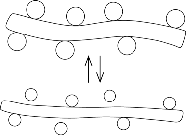
Figure 1: The test tube configuration is a compromise between bending and confinement free energy for fixed positions of the contacts with the surrounding tubes.

The effective building blocks of an entangled semidilute solution of semiflexible polymers are thermal tubes [10]. Their free energy can be decomposed into two contributions: the confinement of long wavelength undulations of the “enclosed” polymer, and tube bending. Any simplified analytical approach relies on a crucial assumption on how macroscopic strains couple to the individual tube. Following Doi and Kuzuu [1] but replacing their rods by tubes, we envision the typical unit-cell as a test tube interacting via freely slipping entanglements with a background of other, identically behaving tubes. The test tube is assumed to be in a local equilibrium for the given, fixed configuration of the background (Fig. 1). Thus the model describes the behaviour on timescales intermediate between the terminal relaxation time and the typical slipping time for the contacts. The fact that the slipping time may be very sensitive to details of the molecular interactions and ambient conditions [2] raises interesting prospects for future developments of the model which we do not pursue further here.

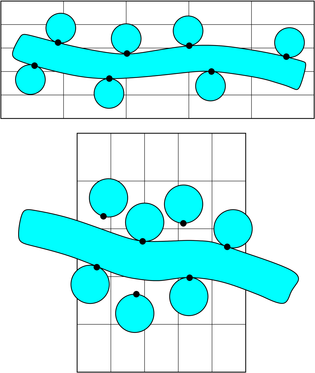
Figure 2: The background deformation is assumed to be affine and volume-preserving. The tube adapts adiabatically to its local free energy minimum. Note that the tube deforms non-affinely although the contact points obey the macroscopic (affine) deformation. The number of contacts may also change as the background is distorted [1].

The major simplifying assumption of the unit-cell model is that the background of the test polymer is bound to deform affinely with the macroscopic deformation given by a deformation tensor ${\bm{\Lambda}}$. Due to the discrete nature of the contacts, the test filament deforms differently from its surroundings. In this way, nonaffinity at the entanglement scale is taken into account in an efficient and transparent approximation (Fig. 2). The affine background has to maintain a constant volume to respect the (effective) incompressibility of the solvent — in terms of the eigenvalues $\lambda_{i}$ of the deformation tensor ${\bm{\Lambda}}$,

$$\lambda_{1}\,\lambda_{2}\,\lambda_{3}=1\;.$$

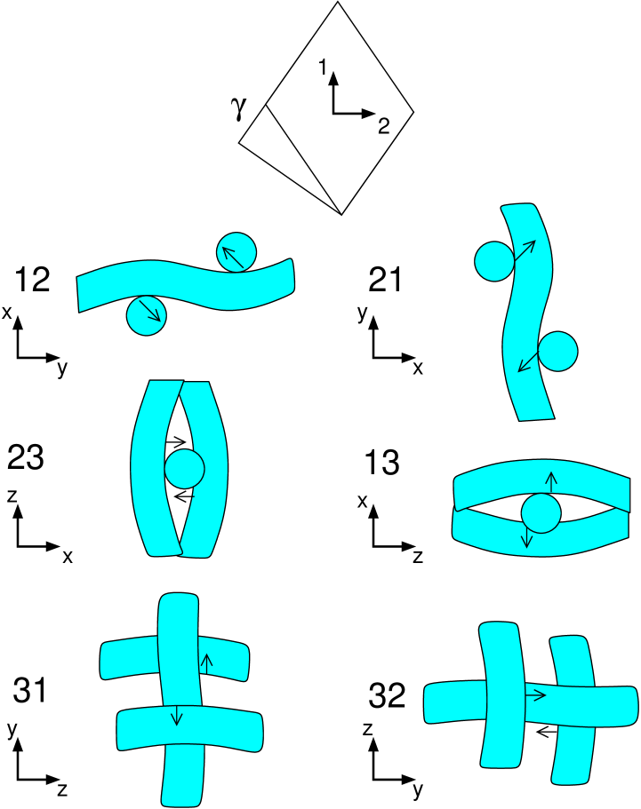
Figure 6: Unit-cell for shear in the 1–2 plane. The main stretch directions 1–2–3 rotate with the current configuration. The unit-cell is modeled as a superposition of test tubes lying along the main stretches. Each configuration is named according to the $x$–$y$ coordinates. The arrows indicate the displacement of the contacts upon an increase of the affine strain $\gamma$.

As a further, merely technical simplification [1] we assume filaments to lie along the eigenvectors of the deformation tensor with a periodic arrangement of contacts with a wavelength given by the mesh size. This simplification has recently been shown to introduce only very minor errors into the equilibrium properties of semiflexible polymer solutions [24] and may be expected to remain uncritical for our purpose. It has the great benefit of allowing for a simple intuitive explanation of the relevant physics in terms of a few paradigmatic cell configurations. Namely, the ensemble of unit-cells to be considered reduces to the six independent realisations depicted in Fig. 6 (see below). Considering the full nonlinear expressions for bending and confinement for these representative realisations, we can then study large deformations.

2.2 The Tube

The free energy

$$\mathcal{A}=\mathcal{A}^{\rm co}+\mathcal{A}^{\rm be}$$

of the test tube is split into the contributions from confinement and bending, $\mathcal{A}^{\rm co}$ and $\mathcal{A}^{\rm be}$, respectively. The confinement free energy of a weakly bending rod constrained by a tube-like harmonic potential of strength $\kappa/(2L_{e}^{4})$ is $k_{B}T$ per collision or “entanglement” length $L_{e}$ [11]. The real constraining potential is clearly not uniform, but rather a discrete set of surrounding tubes. Nevertheless, since the main contribution to the confinement energy comes from the constraint on wavelengths longer than the entanglement length, we may coarse-grain over the contact points and treat the tube as homogeneous, with a (state-dependent) half width

$$\sqrt{\langle\bm{r}_{\!x}^{2}(L_{e})\rangle}\equiv d/2\simeq L_{e}^{3/2}\ell_{p}^{-1/2}\;.$$

For the remainder, we prefer to work in natural units measuring energies in units of thermal energy $k_{B}T$ and lengths as multiples of the persistence length $\ell_{p}$. The confinement free energy of a tube segment of length $\ell$ then takes the form

$$\mathcal{A}^{\rm co}(d,\,\ell)\simeq\>\ell\,d^{-2/3}\;.$$

And the bending energy of the space curve $\bm{r}(s)$ of length $\ell$ representing the tube backbone reads

$$\mathcal{A}^{\rm be}[\bm{r}(s)]=\frac{1}{2}\int\limits_{0}^{\ell}{\rm d}s\Bigg{(}\frac{{\rm d}^{2}\bm{r}}{{\rm d}s^{2}}\Bigg{)}^{2}\;.$$

Taking tube backbones to be elastica [28], the bending energy is automatically at its minimum for given boundary conditions.

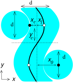
Figure 3: A tube interacting with the surrounding tubes. The tube width is $d$ and its deflection is $x_{\ell}$. Taking advantage of the simple geometry, the cartesian coordinate system is chosen with $x$ along the force $F$ and $y$ perpendicular to the force along the (average) tube axis. Two alternative versions of the central assertion are considered, namely that (1) the contact point (black dot) coordinates $x_{c}$, $y_{c}$ or (2) the obstacle centers $x_{o}$, $y_{o}$ vary affinely with the macroscopic strain.

We intend to describe networks of strongly entangled filaments for which both the total contour length and the persistence length are much longer than the mesh size $\xi$. End-effects at the edges of the tube can thus be neglected. Moreover, for our mean-field theory we may take a periodic arrangement of contacts with a typical distance $\xi$. Since the contacts slip freely, the force of magnitude $F$ acting at these contacts must be perpendicular to the test tube. The simple geometry naturally suggests the cartesian coordinates illustrated in Fig. 3. The coordinate along the force is $x$, and the coordinate along the (average) tube axis is $y$. The point symmetric obstacles have (up to a sign) their center at $x_{o}$, $y_{o}$ and contacts with the test tube at $x_{c}$, $y_{c}$. Their relation to the backbone coordinates $x_{\ell},\,y_{\ell}$ at a “chemical” or arclength distance $\ell$ from the center is read off from Fig. 3,

$$x_{\ell} = x_{o}\pm d=x_{c}\pm d/2$$ (1)

$$y_{\ell} = y_{0}=y_{c}\;,$$ (2)

the sign $\pm$ referring to the sign of $y_{c}$. Because of the symmetry, it is sufficient to concentrate onto the positive sector $y_{c}>0$ with $\pm\to+$.

The initial position of the contacts has an important influence on the elastic response of the unit-cell. The mean separation between contacts along the tube is taken as the entanglement length, $2y_{c}^{0}=L_{e}$. In the direction perpendicular to the tube we assume $x_{c}^{0}=d/2$. Borrowing the equilibrium values for entanglement length and tube diameter from the analysis of the ground state by Hinsch et al [24], our ground state conditions are

$$x^{0}_{c} =-\frac{0.32}{\sqrt{2}}\,\xi^{6/5}$$ (3a)

$$y^{0}_{c} =+\frac{0.66}{2}\,\xi^{4/5}\quad.$$ (3b)

For typical in vitro actin solutions the aspect ratio $y_{c}^{0}/x_{c}^{0}$ has a quite large value of about 7 as a consequence of the small ratio $\xi/\ell_{p}\simeq 0.05$. We remark that this choice of the ground state is only meant as a starting point. We will eventually explore how much the inital aspect ratio affects the stress-strain relation.

We now turn to the calculation of the bending energy for arbitrary states. Within our mean-field description it suffices to consider the problem constrained to the plane. The direction of the force $\bm{F}$ is the natural reference for the tangent angle $\theta$, given by

$$\bm{F}\cdot\frac{{\rm d}\bm{r}}{{\rm d}s}=F\cos(\theta)\;,$$

where $F=|\bm{F}|$ is the magnitude of the external force (in our natural units). The equilibrium equation for an Euler-Bernoulli beam lying in a plane and in absence of body forces is

$$\frac{\rm d^{2}\theta}{{\rm d}s^{2}}=F\sin\theta\;,$$ (4)

the well-known equation of elastica [28]. Its first integral is

$$\frac{1}{2}\,\Bigg{(}\frac{\rm d\theta}{{\rm d}s}\Bigg{)}^{\,2}=F\,\Big{(}\,\cos(\theta_{0})-\cos(\theta)\,\Big{)}\;.$$ (5)

So-called inflexional elastica arise in our theory. Taking an inflexion point (where ${\rm d}\theta/{\rm d}s=0$) as origin, the solution to Eq. 5 can be shown [28] to be given by

$$\cos(\theta/2) =k\,\sin(\phi)$$ (6a)

$$\phi ={\rm am}\big{(}s\sqrt{F}+\mathcal{K};\,k\big{)}\;,$$ (6b)

where ${\rm am}(\>;k)$ is the Jacobi amplitude function with modulus $k$, and the quarter-period $\mathcal{K}$ is implicitly defined by

$${\rm am}(\mathcal{K};\,k)=\pi/2\;.$$

The functional form of the solution is given by $k$, and can be therefore completely defined by the angle $\theta=\theta_{0}$ between beam and force at the inflexion point at the origin, where

$$s=0\;,\qquad\phi=\pi/2\;,\qquad\cos(\theta_{0}/2)=k\;,$$ (7)

holds. That is, the magnitude of the force enters merely as a scale factor for the arclength coordinate $s$ (in our natural units, $F^{-1/2}$ is roughly the arc length that would buckle under the load $F$).

It will be advantageous to introduce cartesian coordinates (see Fig. 3) satisfying

$$\frac{{\rm d}x}{{\rm d}s} =\cos(\theta)$$ (8a)

$$\frac{{\rm d}y}{{\rm d}s} =\sin(\theta)\;.$$ (8b)

The solution can then be written [28] as

$$x_{s} =s-\frac{2}{\sqrt{F}}\,\Bigm{(}\mathcal{E}(\phi\,;k)\>-\>\mathcal{E}(\pi/2;\,k)\Bigm{)}$$ (9a)

$$y_{s} =-\frac{2\,k}{\sqrt{F}}\>\cos(\phi)\;,$$ (9b)

where $\mathcal{E}$ is the elliptic function of the second kind. Setting initial conditions $(\theta,\,{\rm d}\theta/{\rm d}s)$ at a given point $s$ gives a unique solution for the elastica shape. However, the problem is rather one of fulfilling boundary conditions. As illustrated in Fig. 4, they are

$$\frac{\rm d\theta}{{\rm d}s}=0\quad \mbox{at}\quad s=0$$ (10a)

$$\theta=\frac{\pi}{2}\quad \mbox{at}\quad s=\ell\;.$$ (10b)

The first boundary condition is already implicit in the form of the solution.

A simple expression for the bending energy of an elastica segment can be written in cartesian coordinates. Integrating Eq.5 from $s=0$ to $s=\ell$ gives

$$\mathcal{A}^{\rm be}=F\,\bigg{(}\ell\,\cos(\theta_{0})-x_{\ell}\bigg{)}\;.$$ (11)

The tube changes its width and distorts its backbone to reach a free energy minimum for prescribed (affine) coordinates $x_{c},\,y_{c}$ of the contact point. (Alternatively, if the coordinates $x_{o}$, $y_{o}$ are taken to obey the affine deformation, they have to be substituted for $x_{c},\,y_{c}$ in the following discussion.) The free energy extremum equation is thus

$$\frac{\partial\mathcal{A}}{\partial{x_{\ell}}}(x_{\ell},x_{c},y_{c})\Big{|}_{x_{c},\,y_{c}}=0$$ (12)

which gives the equilibrium coordinate $x_{\ell}^{\rm eq}(x_{c},\,y_{c})$ of the tube backbone. In principle, for the free energy minimization we thus have to remove $F$, $\ell$ and $\theta_{0}$ from $\mathcal{A}^{\rm be}$ in Eq. (11) in favour of $x_{c}$, $y_{\ell}=y_{c}$, and $x_{\ell}$. This would require a full inversion of the elliptic functions in Eq. 14. Therefore, in practice, the derivative $\partial_{x_{\ell}}$ has to be rearranged into derivatives with respect to $F$,

$$\frac{\partial\mathcal{A}}{\partial x_{\ell}}^{\!\rm be}\Big{|}_{y_{\ell}}=\frac{\partial\mathcal{A}}{\partial F}^{\!\rm be}\Big{|}_{y_{\ell}}\Bigg{(}\frac{\partial x_{\ell}}{\partial F}\Big{|}_{y_{\ell}}\Bigg{)}^{-1}\;,$$

where all partial derivatives are taken for constant $y_{\ell}$. Accordingly, explicit expressions are only needed for $x_{\ell}(F,\,y_{\ell})$ and $\mathcal{A}^{\rm be}(F,\,y_{\ell})$.

The remainder of the section is devoted to obtaining expressions in terms of $F,\,y_{\ell},\,x_{c}$ as independent variables. Setting $s=\ell$, inverting Eq. 9b and replacing $\phi$ in Eq. 9a gives an expression for $x_{\ell}$ as a function of $k,\,F,\,y_{\ell}$. Inserting the second boundary condition, Eq. 10b, into Eqs. 6 gives

$$\frac{1}{\sqrt{2}}=k\>\sin{{\rm am}\big{(}\ell\sqrt{F}+\mathcal{K};\,k\big{)}}\;.$$ (13)

The (variable) length $\ell$ can be removed by squaring Eqs. 9b and 13 and adding them into

$$k^{2}=\frac{1}{2}+\frac{y_{\ell}^{2}\,F}{4}\;.$$ (14)

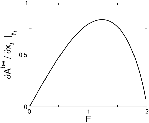
Figure 5: Derivative $\partial\mathcal{A}^{\rm be}/\partial x_{\ell}|_{y_{\ell}}$ as a function of force $F$ at the contact point (in units $k_{b}T\ell_{p}/y_{\ell}^{2}$). Only in the linear regime they can be identified. For large deflections $x_{\ell}\gg y_{\ell}$, the force saturates at $2k_{B}T\ell_{p}/y_{\ell}^{2}$ and the bending energy no longer grows with the backbone coordinate $x_{\ell}$.

This equation can be used in all elliptic functions to replace the modulus $k$ by $F$ and $y_{\ell}$. It is then straightforward to find an analytic (albeit cumbersome) expression for $x_{\ell}(F,\,y_{\ell})$. Similarly, Eqs. 13 and 7 can also be readily inverted to obtain expressions for $\ell$ and $\theta_{0}$. In this way we obtain the desired explicit expression for $\mathcal{A}^{\rm be}(F,\,y_{\ell})$. Figure 5 shows $\partial\mathcal{A}^{\rm be}/\partial x_{\ell}|_{y_{\ell}}$ as a function of $F$. The two are equal for small deformations, $x_{\ell}\ll y_{\ell}$. In this linear regime, sliding of the contact point is irrelevant since the lever arm barely changes, i.e., $\ell\simeq y_{\ell}$. However, as the force approaches the order of magnitude of the spring constant, $F\sim y_{\ell}^{-2}$, the contact point begins to slide noticeably. As $\ell\rightarrow\infty$, force and derivative of the bending energy uncouple:

$$F\rightarrow 2\,y_{\ell}^{-2}\quad,\quad\quad\frac{\partial\mathcal{A}}{\partial x_{\ell}}^{\!\rm be}\Big{|}_{y_{\ell}}\rightarrow 0\;.$$

Since the thermodynamic stress is given by the derivative of the energy, such nonlinear sliding effects can asymptotically lead to a peculiar state where the stress is zero although the filaments are under lateral tension, $F\neq 0$.

A similar rearrangement is necessary for the derivative of the confinement energy, since it depends on $\ell$:

$$\frac{\partial\mathcal{A}}{\partial x_{\ell}}^{\!\rm co}\Big{|}_{y_{c}}=d^{-2/3}\>\frac{\partial\ell}{\partial F}\Big{|}_{y_{c}}\Bigg{(}\frac{\partial x_{\ell}}{\partial F}\Big{|}_{y_{c}}\Bigg{)}^{-1}+\,\ell\;\frac{\partial d^{-2/3}}{\partial d/2\;\;}\;,$$

where we have replaced $y_{\ell}$ by $y_{c}$. By adding the derivatives of bending and confinement energy, we finally obtain an explicit expression for $\partial\mathcal{A}/\partial x_{c}$ as a function of $F,\,y_{\ell}$. The free energy minimization is done by numerically solving Eq.12 for $F$ for the given, state-dependent coordinates $y_{c}$ and $x_{c}$.

The ultimate goal is of course the stress-strain relation $\sigma(\gamma)$, with shear strain $\gamma$. To find an analytic expression for the shear stress $\sigma$, we first decompose the derivative as

$$\sigma=\frac{{\rm d}\mathcal{A}}{{\rm d}\gamma}^{\!\rm eq}=\frac{\partial\mathcal{A}}{\partial x_{c}}^{\!\rm eq}\Big{|}_{y_{c}}\>\frac{{\rm d}x_{c}}{{\rm d}\gamma}+\frac{\partial\mathcal{A}}{\partial y_{c}}^{\!\rm eq}\Big{|}_{x_{c}}\>\frac{{\rm d}y_{c}}{{\rm d}\gamma}\;.$$

The equilibrium free energy can be written in terms of the equilibrium tube deflection $x_{\ell}^{\rm eq}(x_{c},\,y_{c})$ as

$$\mathcal{A}^{\rm eq}(x_{c},\,y_{c})=\mathcal{A}(x_{\ell}^{\rm eq}{\!}_{(x_{c},\,y_{c})},\,x_{c},\,y_{c})\;,$$ (15)

a function of the macroscopic deformation. Taking the derivative with respect to the contact position $x_{c}$ gives

$$\frac{\partial\mathcal{A}}{\partial x_{c}}^{\!\rm eq}\Big{|}_{y_{c}}=\frac{\partial\mathcal{A}}{\partial x_{\ell}}\Big{|}_{x_{c},\,y_{c}}\>\frac{\partial x_{\ell}}{\partial x_{c}}^{\!\rm eq}\Big{|}_{y_{c}}+\frac{\partial\mathcal{A}}{\partial x_{c}}\Big{|}_{y,\,x_{\ell}=x_{\ell}^{\rm eq}}\;.$$

Since the energy is at its minimum for constant contact coordinates (Eq. 12), the first term on the rhs is equal to zero and therefore

$$\frac{\partial\mathcal{A}}{\partial x_{c}}^{\!\rm eq}\Big{|}_{y_{c}}=\frac{\partial\mathcal{A}}{\partial x_{c}}\Big{|}_{y_{c},\,x_{\ell}=x_{\ell}^{\rm eq}}=-\frac{\partial\mathcal{A}}{\partial d/2}^{\!\!\!\!\rm co}\;,$$

where the last equality holds since $\mathcal{A}^{\rm be}$ does not depend on $x_{c}$. One similarly finds

$$\frac{\partial\mathcal{A}}{\partial y_{c}}^{\!\rm eq}\Big{|}_{x_{c}}\!=\>\frac{\partial\mathcal{A}}{\partial y_{c}}^{\!\rm be}\Big{|}_{x_{\ell}}+d^{-2/3}\frac{\partial\ell}{\partial y_{c}}\Bigg{|}_{x_{\ell}}\;.$$

We finally obtain

$$\sigma\,=\,-\frac{\partial\mathcal{A}}{\partial d/2}^{\!\!\!\!\rm co}\;\frac{{\rm d}x_{c}}{{\rm d}\gamma}\;+\\ \Bigg{(}\,\frac{\partial\mathcal{A}}{\partial y_{c}}^{\!\rm be}\Big{|}_{x_{\ell}}+d^{-2/3}\frac{\partial\ell}{\partial y_{c}}\Big{|}_{x_{\ell}}\Bigg{)}\,\!\frac{{\rm d}y_{c}}{{\rm d}\gamma}\;.$$ (16)

We will later use this equation to gain physical insight into the mechanical stability of the solution. Note that derivatives with respect to $y_{c}$ for constant $x_{\ell}$ require again a rearrangement, since we do not have explicit expressions with $x_{\ell}$ as independent variable. For this we need

$$\frac{\partial\mathcal{A}}{\partial y_{c}}^{\!\rm be}\Big{|}_{x_{\ell}}=\>\frac{\partial\mathcal{A}}{\partial y_{c}}^{\!\rm be}\Big{|}_{F}-\>\frac{\partial\mathcal{A}}{\partial F}^{\!\rm be}\Big{|}_{y_{c}}\>\frac{\partial x_{\ell}}{\partial y_{c}}\Big{|}_{F}\>\left(\frac{\partial x_{\ell}}{\partial F}\Big{|}_{y_{c}}\right)^{-1}$$

$$\frac{\partial\ell}{\partial y_{c}}\Big{|}_{x_{\ell}}=\>\frac{\partial\ell}{\partial y_{c}}\Big{|}_{F}-\>\frac{\partial\ell}{\partial F}\Big{|}_{y_{c}}\>\frac{\partial x_{\ell}}{\partial y_{c}}\Big{|}_{F}\>\left(\frac{\partial x_{\ell}}{\partial F}\Big{|}_{y_{c}}\right)^{-1}\>.$$

2.3 The Unit-Cell

We have defined the $x$, $y$, $z$ coordinates as fixed to an arbitrary set of tubes. The test tube lies along $y$ and interacts with background tubes which lie along $z$ and move in the $x$–$y$ plane. For an isotropic network, the unit-cell should be modeled as a superposition of test- and background tubes lying along all possible orientations, integrating the triad $x$–$y$–$z$ over the whole 3D triad-space. However, this would complicate the problem enormously, since triads lying oblique to the main axis of the deformation would distort. To simplify matters we follow Doi and Kuzuu [1] and distribute test- and background tubes only along the main stretch directions (the eigenvectors of the right stretch tensor [29]). Since then tubes remain perpendicular to each other, the deformation can be incorporated in the analytical treatment as a translation of the contact point. The total free energy of the unit-cell is then a sum of 6 terms,

$$\mathcal{A}=\mathcal{A}_{12}+\mathcal{A}_{13}+\mathcal{A}_{21}+\mathcal{A}_{23}+\mathcal{A}_{31}+\mathcal{A}_{32}\quad.$$

We denote configurations by the coordinates of the deformation plane; for a particular tube triad, the free energy is given by $\mathcal{A}_{xy}$. Figure 6 depicts all possible arrangements.

2.4 The deformation

We assume the contact points to deform affinely, going from their initial positions $\bm{{\rm R}}_{c}$ to final positions $\bm{{\rm r}}_{c}$. The assumption of affinity means that the deformation gradient $\bm{\Lambda}=\partial\bm{{\rm r}}_{c}/\partial\bm{{\rm R}}_{c}$, is spatially constant, and thus

$$\bm{{\rm r}}_{c}=\bm{\Lambda\,{\rm R_{c}}}$$

holds for all contact points. With our assumption that the tubes lie along the stretch directions, this statement can be written in terms of the stretch factors as

$$\begin{split}x_{c}&=\lambda_{x}\,x_{c}^{0}\\ y_{c}&=\lambda_{y}\,y_{c}^{0}\;.\end{split}$$

Solving Equation 12 we obtain the equilibrium free energy $\mathcal{A}^{\rm eq}$ as a function of the deformation. The (Cauchy) stress tensor $\bm{\sigma}$ can then be calculated as the derivative of the equilibrium free energy per unit volume,

$$\bm{\sigma}=\det\bm{\Lambda}^{-1}\frac{\partial\mathcal{A}^{\rm eq}/V_{e}}{\partial\bm{\Lambda}}\bm{\Lambda}^{T}\;,$$

where the volume of the unit-cell is taken as

$$V_{e}=\xi^{2}L_{e}\simeq x_{c}^{0}\,{y_{c}^{0}\,}^{2}\;.$$

For concreteness and comparison with experiments we will restrict ourselves to volume preserving shear deformations in the plane 1–2, with positive stretch along 1 and contraction along 2. In terms of the eigenvalues of the strain tensor, $\lambda_{1}\rightarrow\infty$, $\lambda_{2}\rightarrow 0$, and $\lambda_{3}=1$ when $\gamma\rightarrow\infty$. The shear stress is given by

$$\sigma=\frac{\partial\mathcal{A}^{\rm eq}/V_{e}}{\partial\gamma}\;.$$ (17)

Since the ground state is assumed to be the same for all orientations — as expected for an isotropic network — the sum of all stresses must give $\sigma=0$ for $\gamma=0$ for the unit-cell. For shear in the 1–2 plane, it is readily seen that two configurations cancel each other’s stress if they are related by an interchange of the directions $1$, $2$.

2.5 Doi-Kuzuu effect

By “Doi-Kuzuu effect” we mean the change in the number of contacts between filaments due to the deformation [1]. A parallelepiped with sides $2d/\lambda_{x}$, $L/\lambda_{y}$, $L/\lambda_{z}$, assumed to lie along the principal stretches, distorts affinely into a parallelepiped with sides $2d$, $L$, $L$. By construction, the number of filaments lying along $z$ which come into contact with the test rod can be readily shown to be [1]

$$\Delta n=\frac{c}{3}\frac{L^{2}}{\lambda_{y}\lambda_{z}}\left(\frac{2d}{\lambda_{x}}-2d\right)=\frac{2}{3}\,cdL^{2}(1-\lambda_{x}).$$

Thus, as the solution is distorted at constant volume, the number of contacts between rods increases, reducing the lever arm for bending. Assuming stress to be of purely enthalpic nature leads to a pronounced stiffening response [1]. We remark that the material becomes stiffer without the rods ever leaving the linear bending regime, a pure network effect.

Such a general stiffening mechanism is certainly worth considering and can be readily incorporated in our theory. The inverse of the number of contacts per unit length, $L/n$, amounts to the distance $y_{c}$ between contacts. For our purposes, however, the stiff rods have to be replaced by thermal tubes with a variable diameter. For this we recast the original argument in differential form. Replacing $cL/3$ by $1/\xi^{2}$, we get

$$\delta y_{c}=\frac{2\,y_{c}^{2}\,d}{\xi^{2}}\>\delta\lambda_{x}\;.$$

An extra term is needed to address tube thickening in absence of shear, which increases the number of contacts according to

$$\delta y_{c}=-\frac{2\,y_{c}^{2}}{\xi^{2}}\>\delta d\;.$$

The two terms influence the evolution of the distance between contacts, $y_{c}$. Within our mean-field approach it is natural to add them to the affine macroscopic deformation:

$$\delta y_{c}=y_{c}^{0}\>\delta\lambda_{y}+\frac{2\,y_{c}^{2}\,d}{\xi^{2}}\>\delta\lambda_{x}-\frac{2\,y_{c}^{2}}{\xi^{2}}\>\delta d\;.$$ (18)

3 Results

3.1 Softening and instability

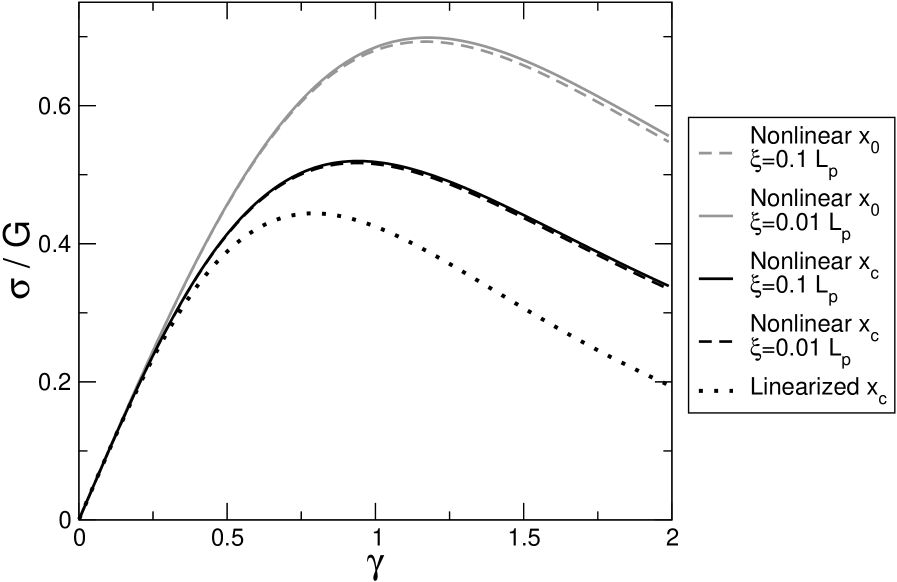
Figure 7: Normalized shear stress-shear strain relation for mesh sizes $\xi/\ell_{p}=0.01$ (solid lines) and $0.1$ (dashed lines). The mesh size barely makes a difference, a consequence of the small filament deflection. The deformation of the background has been considered in two ways. Gray lines: middle points deform affinely, $x_{0}=\lambda_{x}x_{0}^{0}$. Black lines: contact points deform affinely, $x_{c}=\lambda_{x}x_{c}^{0}$. Dotted line: linearized bending energy. For the linearized theory, changing the mesh size merely scales the stress axis.

Figure 7 shows the response of the unit-cell for mesh sizes $\xi/\ell_{p}=0.01$ and $0.1$. The stress-strain relation shows a broad linear regime which softens and becomes unstable beyond 100% shear strain. Though the theory employs the full nonlinear equations for bending, stiffening is not observed, suggesting that the deflection of the test tube remains small throughout. Indeed, linearizing $\mathcal{A}^{\rm be}$ in $x_{\ell}$ around zero has only a minor effect on the stress-strain relation, as shown in Fig. 7. A consequence of the small deflection is that changing the mesh size $\xi$ essentially amounts to a scaling of the stress axis, as can be seen in Fig. 7. For linearized bending the equilibrium deflection scales like $x_{\ell}^{\rm eq}\sim\xi^{4/5}$, which renders both confinement and (linearized) bending energy independent of the mesh size (both are $\sim k_{B}T$). Therefore the stress goes like

$$\sigma=\frac{{\rm d}\mathcal{A}}{{\rm d}\gamma}^{\rm eq,\,lin}\!\!\!\!\!\!\!\!\!\!\!\!(\gamma)\;\Big{/}\;V_{e}(\xi)\sim\xi^{-14/5}\;,$$

which boils down to the well known prediction of the tube model for the concentration dependence of the shear modulus, $G_{0}\sim c^{\,1.4}$. Deviations from this simple mesh-size scaling are a measure of nonlinear bending.

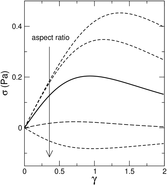
Figure 8: Aspect ratio dependence. Shear stress-shear strain relation for mesh size $\xi=0.02\,\ell_{p}$. The initial aspect ratio $y_{c}^{0}/x_{c}^{0}$ increases along the arrow, taking the values 3.5, 4.9, 7, 10, 14, with $y_{c}^{0}/x_{c}^{0}\approx 7$ corresponding to the tube model, Eq. 3.

A more important parameter is the initial aspect ratio, $y_{c}^{0}/x_{c}^{0}$; as shown in Fig. 8, it decides on the stability of the response. A unit-cell with an aspect ratio larger than $\sim 10$ is already unstable in the ground state. Smaller aspect ratios push the instability away, but without a significant increase in the modulus.

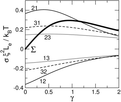
Figure 9: Shear stress versus shear strain for all 6 possible orientations of the test and background tubes, for mesh size $\xi=0.02\,\ell_{p}$. The curve passing through zero stress is the sum of all others, representing the response of the unit-cell. The instability is essentially due to the term 21.

To better understand the mechanical response of the unit-cell in terms of the microscopic deformations, it is helpful to consider the individual contributions of each $xy$ orientation (Fig. 9). In general, none of the individual configurations displays stiffening behaviour. To a varying extent the instability shows up in all contributions. It appears at its strongest in the 2–1-term, corresponding to a test tube along the stretch direction and background tubes along the third direction, moving in the plane 1–2 (see Fig. 6). Since the transverse stiffness of a beam of length $L$ decreases proportional to $L^{-3}$ with increasing length, an increase in the mean distance between adjacent contacts $y_{c}$ weakens the resistance of the test tube, so that its backbone yields to the pressure exerted by the surrounding tubes, which try to expand in order to minimize their confinement free energy. As the deflection of the test tube increases, the negative contribution to the stress from

$$\frac{\partial\mathcal{A}}{\partial y_{c}}^{\!\rm be}\Big{|}_{x_{\ell}}$$

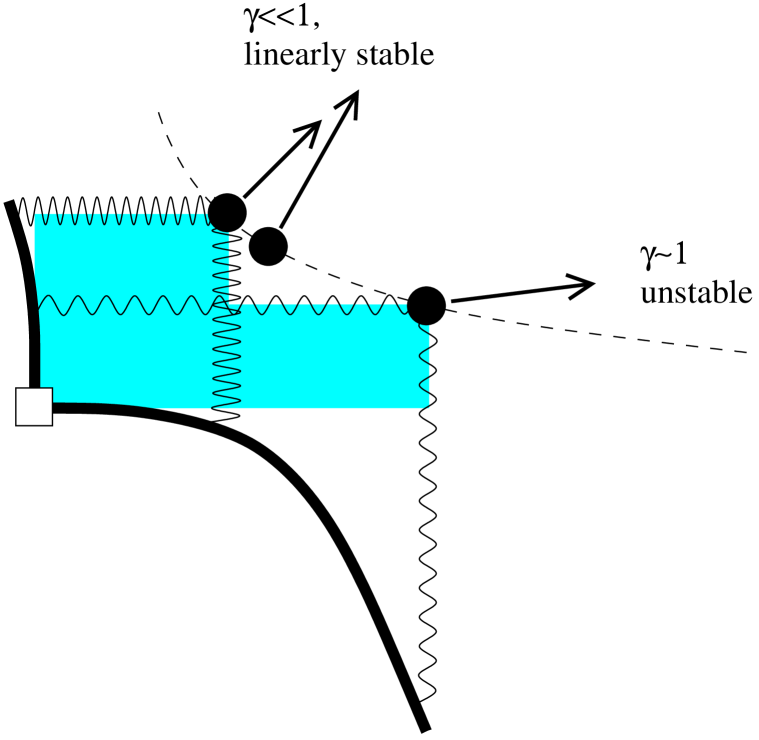
Figure 10: Cartoon illustrating the instability by an intuitive analogy. Due to incompressibility of the shaded area, the contact point (represented by a filled circle) can only move along the dashed line. The springs (representing confinement free energy) have an infinite rest length and slide along clamped beams (representing tube bending). Movement of the contact point increases (lowers) the compression on the spring opposing (favouring) the movement. The arrows correspond to the total force acting on the contact point. In the ground state the lever arm is short and the beams barely bend – the system is linearly stable. As the network is sheared further the increase in lever arm softens the beam, whose bending gives rise to a lateral force pushing out the contact. The system becomes unstable.

will eventually dominate Eq. 16. The instability is an inescapable consequence of our Ansatz for the background deformation and the freely sliding contacts. Figure 10 tries to convey an intuitive feeling for it.

One may wonder whether this instability is an unavoidable feature of stiff polymer solutions or whether higher order correlations neglected in our simple unit-cell approach will eventually stop a real solution from yielding. After all, a living cell should be able to withstand large stretch without collapsing. In the remainder of this section we will digress on two mechanisms which provide stability against large deformations: the Doi-Kuzuu effect [1] and hairpins [25].

3.2 Thermal Doi-Kuzuu effect

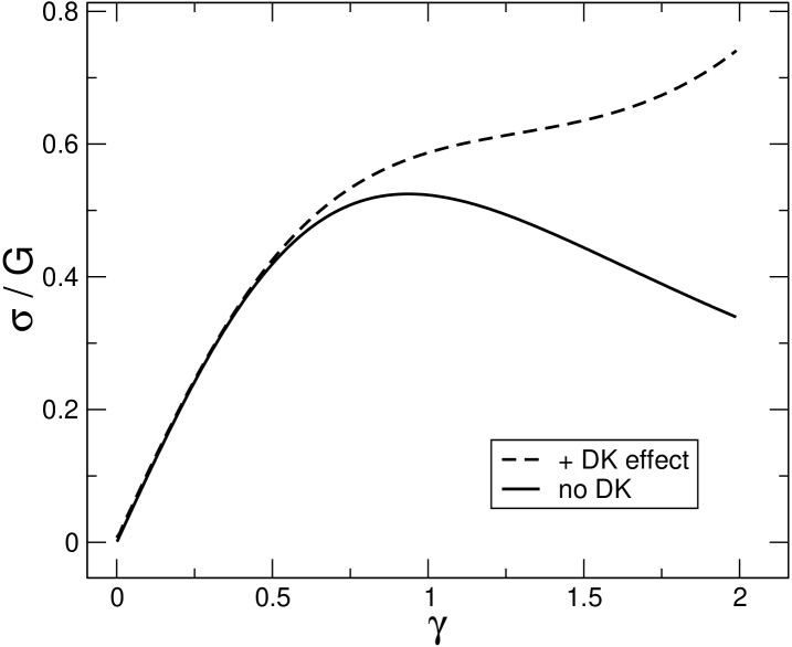
Figure 11: Doi-Kuzuu effect. Shear stress-shear strain relation for mesh size $\xi=0.02\,\ell_{p}$, with and without DK effect. The stiffening response reported in Ref. [1] is “ironed out” by the thermal fluctuations.

The common trend in the results shown so far is a softening response. This seems at odds with the experimentally observed stiffening responses in F-actin solutions [2, 3]. The question arises whether collective effects may be behind them, as in the Doi-Kuzuu effect, which predicts a power-law stiffening response for a solution of rigid rods. As shown in Fig. 11, replacing the rods by tubes with a variable diameter has a dramatic consequence: the stiffening response becomes a softening one. The tug-of-war between Doi-Kuzuu reinforcement via increase in entanglement density and the thermal sliding instability leads to a neutral result where both largely compensate each other. Therefore, though unable to provide stiffening, the Doi-Kuzuu effect renders the unit-cell stable.

3.3 Hairpins are stable

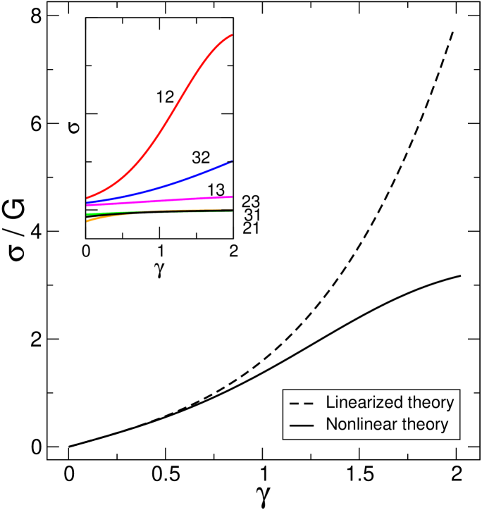
Figure 13: Shear stress versus shear strain for a “hairpin” configuration where $x_{c}>0$, as in Fig. 12. Solid line: full nonlinear theory. Dashed line: linearized theory. The instability vanishes for the hairpin configuration. Note that the weak stiffening response is not due to nonlinear bending, since it is present also in the linearized theory; it is rather a consequence of the decrease of the distance between contacts. Inset: Shear stress versus shear strain for all 6 possible orientations of the test and background tubes.

Here we point out a simple mechanism to stabilize the network even on the level of the single unit-cell. Namely, as depicted in Fig. 12: if the contact $x_{c}$ lies “on the other side”, $x_{c}>0$, such that the test tube is more strongly bent in the ground state. This boils down to a microscopic realization of the “hairpins” first discussed by Morse [25]. Though at first sight innocuous, the change in topology has dramatic consequences for the stress-strain relation. As shown in Fig. 13, the response becomes a weak stiffening one and the sliding instability vanishes. This weak stiffening is not a consequence of nonlinear bending, as can be seen by the response of the linearized theory. Stiffening arises as the distance between contacts and hence the lever arm $y_{c}$ decreases, an effect which dominates for the configuration 1–2 (see Fig. 13, inset). The nonlinear theory actually tames the response into softening at very large shear. This is a consequence of entering a purely sliding regime as in Fig. 5. Thus, though the linearized theory suffices for the typical unit-cell, it grossly overestimates stiffening in the hairpin configuration.

4 Discussion

In the present work we have developed a simple, analytically tractable mean-field description of solutions of stiff biopolymers, describing an adiabatic evolution at timescales longer than typical times for crosslink slippage. The theory makes use of the full nonlinear bending equations and is hence suitable to address large deformations. Surprisingly, in spite of all stiffening mechanisms considered, the theory invariably predicts a broad linear regime which softens and eventually becomes unstable at large shear strain. Nonlinear bending, which leads to strong stiffening responses in the fixed-contact scenario [30], becomes largely irrelevant when contacts slide. The hairpin configuration, though stable, gives a very weak stiffening response which does not resemble the experimental data, where the linear regime does not extend beyond 5% strain [2, 3]. Finally, our version for semiflexible polymers of the geometric Doi-Kuzuu stiffening mechanism [1] is largely cancelled out by thermal fluctuations. Though it does provide stability, the response remains a softening one. We conclude that stiffening in biopolymer solutions necessarily requires coupling to the longitudinal stretching and compression modes of the individual filaments. Our conclusion supports the previous interpretation of stiffening in terms of the glassy wormlike chain [2]. Understood as a consequence of friction, the fact that stiffening requires fast rates and low temperatures and leads to large dissipation makes indeed sense.

Having gained this insight, we can outline a full theory of nonlinear viscoelasticity of biopolymer gels. At fast rates, effectively the solution behaves like a network; here one may expect theories developed for crosslinked networks to hold. Importantly, the elastic strain will be limited to values below $\sim 5\%$ strain, since at larger strains crosslinked networks stiffen dramatically. The large forces attained by the stiffening filaments will break bonds faster and render the deformation inelastic. Thus, for finite rates we expect the nonlinear response to go in hand with huge structural dissipation. As the rate is lowered to timescales intermediate between crosslink slippage and terminal relaxation, the present theory should hold, predicting an almost reversible response, with a broad linear regime. This picture is indeed corroborated by experiments. Both for living cells [8, 9, 31, 32] and in-vitro F-actin solutions [2, 3], stress-strain relations become increasingly linear over large deformations as the strain rate is lowered, and the reversibility of the response increases as dissipation goes down. Thus, there seems to be hope of a unified description of this plethora of mechanical responses in terms of networks of semiflexible filaments with frictional interactions.

As the deformation spreads the contacts along the main stretch axis, their lever arm increases and the test tube no longer can sustain the thermal fluctuations. This leads to a sliding instability and presumably to shear banding at a critical strain of 100%. This picture provides a fresh, novel look at the mysterious “collapse” of biopolymer networks and solutions. Pure F-actin solutions undergo irreversible weakening at $\sim 150\%$ [2, 3]. The experimental fact that this collapse takes place at a well defined strain, largely independent of rate and stress, makes the case for a purely geometrical instability, unrelated to breakage of filaments, possibly resembling collective rearrangements in oil tubes [33]. Though the full nonlinear theory including the coupling to the longitudinal polymer modes is still under development [34], the reasoning outlined above supports the sliding stability as a qualitative explanation for the collapse. Indeed, since the sliding instability takes place at strains $\sim 100\%$ in our theory, and the backbone strain cannot be much larger than 5%, one would expect the critical collapse strain to be largely unaffected by the degree of stiffening, i.e., by the strain rate – as experimentally observed.

Hairpin-entanglements are interesting, as they are stable against large deformations. In fact, these hairpins are always present with a certain small probability on the scale of the unit-cell, and with higher probability on larger scales. Closely related to the hairpins described by Morse in long filaments [25], they have a drastic effect onto the mechanical response, because their deformation and free energy invariably increase upon affine background deformations. By addressing hairpins and normal entanglements separately, their opposite responses at large strains stand out. The instability of the unit-cell against shear may be turned into a weak stiffening response upon changing the entanglement topology to a hairpin. One may therefore wonder whether hairpins are behind the fact that the conspicuous in-vitro collapse is not observed when straining living cells by over 100% [9, 8]. Since large deformations of this order are to be expected under physiological conditions (as cells crawl and divide), it seems desirable to avoid a collapse of the main load-bearing structure in the cell. Though typical actin filament sizes are probably too short to provide strongly bent tubes, one may create hairpins in alternative ways. To achieve the right “inside-out” topology, it would suffice to crosslink filaments at a large angle and let them polymerize, thereby effectively generating a large bent in the ground state. Such a strategy would remind of the Arp 2/3 complex, an ubiquitous component of the actin cortex. As a more generic possible mechanism one can imagine a pre-bending of filaments in the ground state enforced by mutual adhesive interactions or simply by their embedding into a disordered environment. This would provide an intimate link between the question of mechanical stability of living cells and tissues and a fundamental polymer physics problem.

We are very grateful to Andreas R. Bausch for his generous support. Insightful discussions with C. Semmrich and J. Glaser are also acknowledged.

• The test tube configuration is a compromise between bending and confinement free energy for fixed positions of the contacts with the surrounding tubes.

• The background deformation is assumed to be affine and volume-preserving. The tube adapts adiabatically to its local free energy minimum. Note that the tube deforms non-affinely although the contact points obey the macroscopic (affine) deformation. The number of contacts may also change as the background is distorted [1].

• A tube interacting with the surrounding tubes. The tube width is $d$ and its deflection is $x_{\ell}$. Taking advantage of the simple geometry, the cartesian coordinate system is chosen with $x$ along the force $F$ and $y$ perpendicular to the force along the (average) tube axis. Two alternative versions of the central assertion are considered, namely that (1) the contact point (black dot) coordinates $x_{c}$, $y_{c}$ or (2) the obstacle centers $x_{o}$, $y_{o}$ vary affinely with the macroscopic strain.

• Boundary conditions for the tube backbone. At the origin, $s=0$, symmetry requires zero curvature, $d\theta/ds=0$. Since the entanglement at $s=\ell$ slips freely, the force $F$ must be perpendicular to the tangent; i.e., $\theta_{\ell}=\pi/2$.

• Derivative $\partial\mathcal{A}^{\rm be}/\partial x_{\ell}|_{y_{\ell}}$ as a function of force $F$ at the contact point (in units $k_{b}T\ell_{p}/y_{\ell}^{2}$). Only in the linear regime they can be identified. For large deflections $x_{\ell}\gg y_{\ell}$, the force saturates at $2k_{B}T\ell_{p}/y_{\ell}^{2}$ and the bending energy no longer grows with the backbone coordinate $x_{\ell}$.

• Unit-cell for shear in the 1–2 plane. The main stretch directions 1–2–3 rotate with the current configuration. The unit-cell is modeled as a superposition of test tubes lying along the main stretches. Each configuration is named according to the $x$–$y$ coordinates. The arrows indicate the displacement of the contacts upon an increase of the affine strain $\gamma$.

• Normalized shear stress-shear strain relation for mesh sizes $\xi/\ell_{p}=0.01$ (solid lines) and $0.1$ (dashed lines). The mesh size barely makes a difference, a consequence of the small filament deflection. The deformation of the background has been considered in two ways. Gray lines: middle points deform affinely, $x_{0}=\lambda_{x}x_{0}^{0}$. Black lines: contact points deform affinely, $x_{c}=\lambda_{x}x_{c}^{0}$. Dotted line: linearized bending energy. For the linearized theory, changing the mesh size merely scales the stress axis.

• Aspect ratio dependence. Shear stress-shear strain relation for mesh size $\xi=0.02\,\ell_{p}$. The initial aspect ratio $y_{c}^{0}/x_{c}^{0}$ increases along the arrow, taking the values 3.5, 4.9, 7, 10, 14, with $y_{c}^{0}/x_{c}^{0}\approx 7$ corresponding to the tube model, Eq. 3.

• Shear stress versus shear strain for all 6 possible orientations of the test and background tubes, for mesh size $\xi=0.02\,\ell_{p}$. The curve passing through zero stress is the sum of all others, representing the response of the unit-cell. The instability is essentially due to the term 21.

• Cartoon illustrating the instability by an intuitive analogy. Due to incompressibility of the shaded area, the contact point (represented by a filled circle) can only move along the dashed line. The springs (representing confinement free energy) have an infinite rest length and slide along clamped beams (representing tube bending). Movement of the contact point increases (lowers) the compression on the spring opposing (favouring) the movement. The arrows correspond to the total force acting on the contact point. In the ground state the lever arm is short and the beams barely bend – the system is linearly stable. As the network is sheared further the increase in lever arm softens the beam, whose bending gives rise to a lateral force pushing out the contact. The system becomes unstable.

• Doi-Kuzuu effect. Shear stress-shear strain relation for mesh size $\xi=0.02\,\ell_{p}$, with and without DK effect. The stiffening response reported in Ref. [1] is “ironed out” by the thermal fluctuations.

• A hairpin. Setting $x_{c}^{0}>0$, while still complying with the requirement $\lvert x_{c}^{0}\rvert\lvert y_{c}^{0}\rvert\simeq\xi^{2}$, leads to a very different response. Since now the tubes are “trapped”, the entangled solution is stable against large deformations.

• Shear stress versus shear strain for a hairpin configuration where $x_{c}>0$, as in Fig. 12. Solid line: full nonlinear theory. Dashed line: linearized theory. The instability vanishes for the hairpin configuration. Note that the weak stiffening response is not due to nonlinear bending, since it is present also in the linearized theory; it is rather a consequence of the decrease of the distance between contacts. Inset: Shear stress versus shear strain for all 6 possible orientations of the test and background tubes.

Figure 4: Boundary conditions for the tube backbone. At the origin, $s=0$, symmetry requires zero curvature, $d\theta/ds=0$. Since the entanglement at $s=\ell$ slips freely, the force $F$ must be perpendicular to the tangent; i.e., $\theta_{\ell}=\pi/2$.

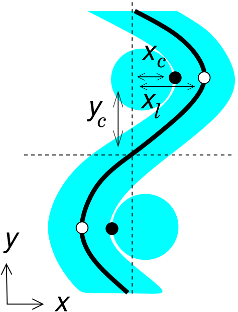
Figure 12: A “hairpin”. Setting $x_{c}^{0}>0$, while still complying with the requirement $\lvert x_{c}^{0}\rvert\lvert y_{c}^{0}\rvert\simeq\xi^{2}$, leads to a very different response. Since now the tubes are “trapped”, the entangled solution is stable against large deformations.

References

- [1] M. Doi and N. Kuzuu, J. Polymer Sci.: Polymer Phys. Ed., 1980, 18, 409–419.
- [2] C. Semmrich, T. Storz, J. Glaser, R. Merkel, A. R. Bausch, and K. Kroy, Proc. Natl. Acad. Sci. USA, 2007, 104(51), 20199–20203.
- [3] C. Semmrich, R. J. Larsen, and A. R. Bausch, Soft Matter, 2008, 4, 1675–1680.
- [4] A. R. Bausch and K. Kroy, Nature Physics, 2006, 2, 231–238.
- [5] D. Bray, Cell Movements: from molecules to motility, Garland Publishing, Inc., New York, 2nd ed., 2001.
- [6] B. Fabry, G. N. Maksym, J. P. Butler, M. Glogauer, D. Navajas, and J. J. Fredberg, Phys. Rev. Lett., 2001, 87(14), 148102.
- [7] X. Trepat, L. Deng, S. S. An, D. Navajas, D. J. Tschumperlin, W. T. Gerthoffer, J. P. Butler, and J. J. Fredberg, Nature, 2007, 447, 592–595.
- [8] P. Fernández, L. Heymann, A. Ott, N. Aksel, and P. A. Pullarkat, New J. Phys., 2007, 9, 419.
- [9] P. Fernández and A. Ott, Phys. Rev. Lett., 2008, 100, 238102.
- [10] K. Kroy, Curr. Opin. Coll. Int. Sci., 2006, 11, 56–64.
- [11] T. Odijk, Macromolecules, 1983, 16, 1340.
- [12] C. Storm, J. J. Pastore, F. C. MacKintosh, T. C. Lubensky, and P. A. Janmey, Nature, 2005, 435, 191–194.
- [13] A. Kabla and L. Mahadevan, J. R. Soc. Interface, 2007, 4, 99–106.
- [14] E. Kuhl, K. Garikipati, E. M. Arruda, and K. Grosh, J. Mech. Phys. Solids, 2005, 53, 1552–1573.
- [15] D. A. Head, A. J. Levine, and F. C. MacKintosh, Phys. Rev. E, 2003, 68, 061907.
- [16] C. Heussinger and E. Frey, Phys. Rev. Lett., 2006, 96(1), 017802.
- [17] C. Heussinger and E. Frey, Phys. Rev. E, 2007, 75, 011917.
- [18] J. Wilhelm and E. Frey, Phys. Rev. Lett., 2003, 91(10), 108103.
- [19] D. A. Head, A. J. Levine, and F. C. MacKintosh, Phys. Rev. Lett., 2003, 91(10), 108102.
- [20] P. R. Onck, T. Koeman, T. van Dillen, and E. van der Giessen, Phys. Rev. Lett., 2005, 95, 178102.
- [21] D. Rodney, M. Fivel, and R. Dendievel, Phys. Rev. Lett., 2005, 95, 108004.
- [22] M. Das, F. Mackintosh, and A. J. Levine, Phys. Rev. Lett., 2007, 99, 038101.
- [23] B. A. DiDonna and T. C. Lubensky, Phys. Rev. E, 2005, 72, 066619.
- [24] H. Hinsch, J. Wilhelm, and E. Frey, Eur. Phys J. E, 2007, 24, 35–46.
- [25] D. C. Morse, Macromolecules, 1999, 32, 5934.
- [26] W. Helfrich, Z. Naturforsch., 1978, 33a, 305–315.
- [27] B. Wagner, R. Tharmann, I. Haase, M. Fischer, and A. R. Bausch, Proc. Natl. Acad. Sci. USA, 2006, 103(38), 13974–13978.
- [28] A. E. H. Love, A treatise on the mathematical theory of elasticity, Dover, New York, 1944.
- [29] M. F. Beatty, Appl. Mech. Rev., 1987, 40(12), 1699–1734.
- [30] P. Fernández, P. A. Pullarkat, and A. Ott, Biophys. J., 2006, 90(9), 3796–3805.
- [31] T. Wakatsuki, M. S. Kolodney, G. I. Zahalak, and E. L. Elson, Biophys. J., 2000, 79, 2353–2368.
- [32] S. Yang and T. Saif, Exp. Cell Res., 2005, 305, 42–50.
- [33] T. Bauer, J. Oberdisse, and L. Ramos, Phys. Rev. Lett., 2006, 97, 258303.
- [34] P. Fernández and K. Kroy, in preparation, 2008.
-
Fig. 1