Testing Flavor Symmetries by B-Factory

Abstract

The Cabibbo-Kobayashi-Maskawa (CKM) parameters are investigated in detail in recent predictive models which are based on low-energy non-abelian discrete family symmetries. Some of the models can already be excluded at the present precision of the determination of the CKM parameters, while some of them seem to survive. We find that to make the uncertainties of the theoretical values comparable with the assumed uncertainties of $\sim 1^{\circ}$ and $\sim 2^{\circ}$ in $\phi_{2}(\alpha)$ and $\phi_{3}(\gamma)$, respectively, at about 50 inverse atto barn achieved at a future B factory, it is necessary to reduce the uncertainties in the quark masses, especially that of the strange quark mass by more than 60%.

I Introduction

The success of the standard model (SM) suggests that we are very close to a more fundamental theory for elementary particle physics. Yet, we do not know how the SM should be extended, except that the mass of neutrinos with their mixing and a dark matter candidate have to be incorporated in the extension. The Higgs sector of the SM indicates that the extension may take place around TeV scale, and supersymmetry is widely believed to be the best candidate to increase the natural energy scale of the theory. Yet another problem is the Yukawa sector, because the most of the free parameters of the SM are involved there and the SM does not provide with a principle how to fix its structure. Moreover, simple supersymmetry does not soften the problem of the Yukawa sector.

A natural way to provide with a principle for the Yukawa sector is the introduction of a family symmetry. A family symmetry is not necessarily adequate to explain the observed hierarchy of the fermion masses. It can however relate the fermion masses and mixing parameters. That is, mixing parameters may be related to mass ratios. Note that the classic relations such as $\sin\theta_{C}\simeq\sqrt{m_{d}/m_{s}}$ Gatto:1968ss ; Cabibbo:1968vn ; Fritzsch:1977za , or $|V_{ub}/V_{cb}|\simeq\sqrt{m_{u}/m_{c}}$ Hall:1993ni ; Roberts:2001zy Ramond:1993kv had not been derived from a family symmetry. Recently there have been a growing number of interests in family symmetries. Most of the recent papers deal with the large neutrino mixing (see for instance Altarelli:2007gb ; Ma:2004pt ; Lam:2008sh ), because a large mixing may be associated with a family symmetry. As for the quark masses and mixing, tremendous works on their ansatz have been done (see for instance Fritzsch:1999ee ). However, there is an almost no-go theorem Koide:2004rd saying that there exists no viable low-energy family symmetry in the SM to understand the fermion mass matrices. Therefore, if the fermion mass matrices should be derived from a family symmetry, one has to extend the SM. One of the possibilities is to extend the Higgs sector such that it also forms a family Pakvasa:1977in . In fact a renewed interest in this approach to the quark sector has been recently aroused Ma:2002yp -Ishimori:2008fi .

In this paper we are interested in predictive flavor models with a low-energy discrete family symmetry that are testable at future B factories such as SuperKEKB Akeroyd:2004mj and Super Flavour Factory Browder:2007gg . We met a set of the following selection criteria for the models:
1) The family symmetry should be a low-energy symmetry. That is, we do not include here family symmetries at GUT scale.
2) The family symmetry should not be hardly broken. If it is hardly broken, there is in general no quantitative prediction of the symmetry. So, we do not consider textures which are not supported by a symmetry.
3) The model should describe 10 observables, six quark masses and four Cabibbo-Kobayashi-Maskawa (CKM) parameters, by less than 10 parameters.
4) The model should be renormalizable.
To our knowledge there are only four models proposed in Lavoura:2005kx ; Chen:2005jt ; Babu:2004tn that satisfy the selection criteria above.

In the next section we will start by summarizing the present values of the CKM parameters and quark masses. We will find that the uncertainties in the light quark masses have to be largely reduced to make the uncertainties of the theoretical values of the CKM parameters comparable with the assumed experimental uncertainties of future B factories. The lattice calculation Blum:2007cy is indeed an on-going project to reduce the uncertainties in the light quark masses. In this paper, however, we will not use the quark mass values given in Blum:2007cy , because the uncertainties due to the absence of the sea strange quarks have not been included.

II Quark masses and CKM parameters

Our strategy to compare the theoretical values with the experimental ones is to use the six quark masses along with two of the CKM parameters to plot the theoretical values in the plane defined by other two CKM parameters. From the quark masses in the $\overline{\mbox{MS}}$ scheme given in Particle Data Group 2009 Amsler:2008zz we obtain the quark masses at $\mu=M_{Z}$ Kim:2004ki

$$m_{u}(M_{Z})=0.98\sim 2.15\ {\rm MeV}~{},~{}m_{d}(M_{Z})=2.28\sim 3.90\ {\rm MeV},$$

$$m_{s}(M_{Z})=45.5\sim 84.5\ {\rm MeV}~{},~{}m_{c}(M_{Z})=0.65\sim 0.75\ {\rm GeV},$$ (1)

$$m_{b}(M_{Z})=2.85\sim 3.02\ {\rm GeV}~{},~{}m_{t}(M_{Z})=179.2\sim 183.7\ {\rm GeV}.$$

The input parameters we shall use are the ratios at $\mu=M_{Z}$, i.e.

$$m_{u}/m_{t}=(0.54\sim 1.18)\times 10^{-5}~{},~{}m_{c}/m_{t}=(0.36\sim 0.41)\times 10^{-2},$$

$$m_{d}/m_{b}=(0.79\sim 1.34)\times 10^{-3}~{},~{}m_{s}/m_{b}=(0.16\sim 0.29)\times 10^{-1}.$$ (2)

Given the ratios above, there are two independent mass scales, one for the up quarks and the other for the down quarks: if necessary we use the fixed values $m_{b}(M_{Z})=2.9\ {\rm GeV}\ ,\ m_{t}(M_{Z})=181.4\ {\rm GeV}$. We further require that Amsler:2008zz

$$m_{s}/m_{d}=17\sim 22~{},~{}\frac{m_{u}+m_{d}}{2}=2.5\sim 5.5\ {\rm MeV}~{},~{}\frac{2m_{s}}{m_{u}+m_{d}}=25\sim 30~{},~{}$$

$$m_{u}/m_{d}=0.35\sim 0.6~{},~{}\frac{m_{s}-(m_{u}+m_{d})/2}{m_{d}-m_{u}}=30\sim 50$$ (3)

are satisfied. We also use

$$|V_{us}|=0.2236\sim 0.2274~{},~{}|V_{cb}|=0.0401\sim 0.0423$$ (4)

as the two input parameters of the CKM parameters. Then the theoretical values are compared with two sets of the experimental values:

PDG:Amsler:2008zz

$$\bar{\rho}=0.1425\pm 0.0235~{},~{}\bar{\eta}=0.348\pm 0.016,$$

$$\phi_{2}(\alpha)=(88.5\pm 5.5)^{\circ}~{},~{}\phi_{3}(\gamma)=(76\pm 31)^{\circ}~{},~{}\sin 2\phi_{1}(\beta)=(0.681\pm 0.025),$$ (5)

$$|V_{ub}|=(3.93\pm 0.36)\times 10^{-3}~{},~{}|V_{td}/V_{ts}|=0.209\pm 0.007,$$

and

UTFit:utfit

$$\bar{\rho}=0.154\pm 0.022~{},~{}\bar{\eta}=0.342\pm 0.014,$$

$$\phi_{2}(\alpha)=(92.0\pm 3.4)^{\circ}~{},~{}\phi_{3}(\gamma)=(65.6\pm 3.3)^{\circ}~{},~{}\sin 2\phi_{1}(\beta)=0.695\pm 0.020,$$ (6)

$$|V_{ub}|=(3.60\pm 0.12)\times 10^{-3}~{},~{}|V_{td}/V_{ts}|=0.209\pm 0.0075.$$

III The models and their CKM parameters

In this section we consider four different flavor models with three different family symmetries. Except the model II of Chen:2005jt these models should be supersymmetric to obtain desired mass matrices for the quarks. The family symmetry of the models III and IV of Babu:2004tn extends to the leptonic sector so that there are nontrivial, testable predictions in that sector, too. The $SU(2)_{L}$ doublets of the quarks and Higgs bosons are denoted by $Q$ and $H^{u,d}$, respectively. Similarly, $SU(2)_{L}$ singlets of the quarks are denoted by $U^{c}$ and $D^{c}$. In the supersymmetric models they are superfields, and they are ordinary fields in the non-supersymmetric case.

III.1 The model I Lavoura:2005kx

	$Q_{1,2}\ U^{c}_{1,2}\ D^{c}_{1,2}$	$H^{u}_{1,2}$	$H^{d}_{1,2}$	$Q_{3}\ U^{c}_{3}\ D^{c}_{3}$	$H^{u}_{3}\ H^{d}_{3}$
$S_{3}$	2	2	2	1	1
$Z_{2}$	1	$-1$	1	$-1$	1

Table 1: The $S_{3}$ and $Z_{2}$ assignment in the model I. Lavoura:2005kx

The first model, which is proposed in Lavoura:2005kx , is the supersymmetric model with an $S_{3}\times Z_{2}$ family symmetry. The $S_{3}\times Z_{2}$ assignment is given in Table 1, and the $S_{3}\times Z_{2}$ invariant cubic superpotential for the Yukawa interactions in the quark sector is given by

$$W_{q}=Y^{u}_{a}Q_{3}U^{c}_{3}H^{u}_{3}+Y^{u}_{b}(Q_{1}H^{u}_{2}+Q_{2}H^{u}_{1})U^{c}_{3}$$

$$\hskip 28.45274pt+Y^{u}_{c}Q_{3}(U^{c}_{1}H^{u}_{2}+U^{c}_{2}H^{u}_{1})+Y^{u}_{e}(Q_{1}U^{c}_{2}+Q_{2}U^{c}_{1})H^{u}_{3}$$

$$\hskip 28.45274pt+Y^{d}_{a}Q_{3}D^{c}_{3}H^{d}_{3}+Y^{d}_{e}(Q_{1}D^{c}_{2}+Q_{2}D^{c}_{1})H^{d}_{3}+Y^{d}_{f}\left(Q_{2}D^{c}_{2}H^{d}_{2}+Q_{1}D^{c}_{1}H^{d}_{1}\right)\ ,$$ (7)

where the subscripts $1,2$ and $3$ stand for the two components of the $S_{3}$ doublet and for the $S_{3}$ singlet, respectively.

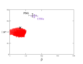
Figure 1: The theoretical values of the model I at $90\%$ CL in the $\bar{\rho}{\bf-}\bar{\eta}$ plane. Two experimental values (5) and (6) are also plotted. The best fit point is denoted as $\times$.

After the spontaneous electroweak symmetry breaking, the Higgs doublets should acquire vacuum expectation values (VEVs) $<H_{i}^{u,d}>=v_{i}^{u,d}$. Then the quark mass matrices are

$$M_{u}=\left(\begin{array}[]{ccc}0&Y^{u}_{e}\ v^{u}_{3}&0\\ Y^{u}_{e}\ v^{u}_{3}&0&Y^{u}_{b}\ v^{u}_{1}\\ 0&Y^{u}_{c}\ v^{u}_{1}&Y^{u}_{a}\ v^{u}_{3}\end{array}\right)\equiv\left(\begin{array}[]{ccc}0&x&0\\ x&0&z\\ 0&y&w\end{array}\right)\ ,$$ (14)

$$M_{d}=\left(\begin{array}[]{ccc}0&Y^{d}_{e}\ v^{d}_{3}&0\\ Y^{d}_{e}\ v^{d}_{3}&Y^{d}_{f}\ v^{d}_{2}&0\\ 0&0&Y^{d}_{a}\ v^{d}_{3}\end{array}\right)\equiv\left(\begin{array}[]{ccc}0&p&0\\ p&q&0\\ 0&0&m_{b}\end{array}\right)\ .$$ (21)

Note that $v_{2}^{u}=v_{1}^{d}=0$ is assumed, and supersymmetry makes it possible to obtain this relation naturally Lavoura:2005kx .

All the elements of these matrices can be made real and positive by an appropriate redefinition of the quark fields. Therefore, the real quark mass matrices can be diagonalized by orthogonal matrices as follows,

$$O_{u}^{T}M_{u}M_{u}^{T}O_{u}={\rm diag}(m_{u}^{2},m_{c}^{2},m_{t}^{2})\ ,$$ (22)

$$O_{d}^{T}M_{d}M_{d}^{T}O_{d}={\rm diag}(m_{d}^{2},m_{s}^{2},m_{b}^{2})\ ,$$ (23)

and the CKM matrix is written as

$$V=O_{u}^{T}PO_{d}\ ,$$ (24)

where $P={\rm diag}(1,e^{i\phi},1)$. There are only eight independent parameters, so that we can calculate two remaining physical quantities.

The CKM matrix $V$ can be approximately obtained in a closed form, and one finds Lavoura:2005kx , for instance,

$$\left|\frac{V_{ub}}{V_{cb}}\right|\simeq\frac{xw}{yz}\simeq\sqrt{\frac{m_{u}}{m_{c}}}~{},~{}\frac{V_{td}}{V_{ts}}\simeq-\tan\alpha_{d}\simeq-\sqrt{\frac{m_{d}}{m_{s}}}\ .$$ (25)

Using the values given in (1), (2) and (4), we find

$$|V_{ub}|\simeq|V_{cb}|\sqrt{\frac{m_{u}}{m_{c}}}\simeq(1.4\sim 2.4)\times 10^{-3}\ ,$$ (26)

$$\left|\frac{V_{td}}{V_{ts}}\right|\simeq\sqrt{\frac{m_{d}}{m_{s}}}\simeq 0.213\sim 0.242\ .$$ (27)

As we can see from (5) and (6), the ratio $\left|V_{td}/V_{ts}\right|$ is consistent with the experimental value, while $|V_{ub}|$ is not. We have performed a systematic, numerical analysis of the theoretical values in various planes. Fig. 1 shows the case of the model I at $90\%$ CL in the $\bar{\rho}{\bf-}\bar{\eta}$ plane. We clearly see that the model I is not consistent with the experimental observations.

III.2 The model II Chen:2005jt

	$\bar{Q}_{1,2}\ d_{1,2}$	$u_{1,2}$	$H^{d}_{1,2}$	$H^{u}_{1,2}$	$\bar{Q}_{3}\ d_{3}\ u_{3}$	$H^{d}_{3}\ H^{u}_{3}$
$D_{7}$	2	$\bf 2^{{}^{\prime}}$	2	$\bf 2^{{}^{\prime\prime}}$	1	1

Table 2: $D_{7}$ assignments of the matter fields.

Next we consider the $D_{7}$ flavor symmetric model of Chen:2005jt , where a supersymmetric extension is not always necessary in this model. The $D_{7}$ assignment is given in Table 2, and the $D_{7}$ invariant Yukawa Lagrangian of the quark sector can be written as

$${\cal L}_{q} = Y_{a}^{u}(\bar{Q}_{2}H_{1}^{u}d_{2}+\bar{Q}_{1}H_{2}^{u}u_{1})+Y_{b}^{u}Q_{3}H_{3}^{u}u_{3}$$ (28)

$$+Y_{a}^{d}(\bar{Q}_{1}d_{2}+\bar{Q}_{2}d_{1})H_{3}^{d}+Y_{b}^{d}(\bar{Q}_{1}H_{2}+\bar{Q}_{2}H_{1}^{d})d_{3}$$

$$+Y_{c}^{d}\bar{Q}_{3}(H_{1}^{d}d_{2}+H_{2}^{d}d_{1})+Y_{e}^{d}\bar{Q}_{3}H_{3}^{d}d_{3}+h.c.\ ,$$

which yields the quark mass matrices of the form

$$M_{u}=\left(\begin{array}[]{ccc}Y_{a}^{u}\ v^{u}_{2}&0&0\\ 0&Y_{a}^{u}\ v^{u}_{1}&0\\ 0&0&Y_{b}^{u}\ v^{u}_{3}\end{array}\right)\equiv\left(\begin{array}[]{ccc}m_{u}&0&0\\ 0&m_{c}&0\\ 0&0&m_{t}\end{array}\right)\ ,$$ (35)

$$M_{d}=\left(\begin{array}[]{ccc}0&Y_{a}^{d}\ v^{d}_{3}&Y_{b}^{d}\ v^{d}_{2}\\ Y_{a}^{d}\ v^{d}_{3}&0&Y_{b}^{d}\ v^{d}_{1}\\ Y_{c}^{d}\ v^{d}_{2}&Y_{c}^{d}\ v^{d}_{1}&Y_{e}^{d}\ v^{d}_{3}\end{array}\right)\equiv\left(\begin{array}[]{ccc}0&a&\xi b\\ a&0&b\\ \xi c&c&d\end{array}\right)\ ,$$ (42)

where $<H^{u,d}_{i}>\equiv v^{u,d}_{i}$. Except for $\xi$, the parameters $a,b,c$ and $d$ of $M_{d}$ can be made real and positive. That is, there are nine independent parameters in the quark sector, and we can calculate one physical quantity.

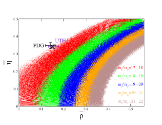
Figure 2: The theoretical values of the model II at $90\%$ CL in the $\bar{\rho}{\bf-}\bar{\eta}$ plane. Different colors indicate different intervals of the mass ratio $m_{s}/m_{d}$: $17\sim 18$ (red), $18\sim 19$ (green), $19\sim 20$ (blue), $20\sim 21$ (orange), and $21\sim 22$ (brown). Two experimental values (5) and (6) are also plotted. The best fit point of the model II is denoted as $\times$.

The mass matrix of the down quarks can be diagonalized by a unitary matrix $V_{d}$ as

$$V_{d}^{{\dagger}}M_{d}M_{d}^{{\dagger}}V_{d}={\rm diag}(m_{d}^{2},m_{s}^{2},m_{b}^{2})\ ,$$ (43)

and the CKM matrix is then given by

$$V=V_{d}\ ,$$ (44)

because the mass matrix of the up quarks $M_{u}$ is diagonal, which is a consequence of the family symmetry. If one assumes that $a^{2}\ll b^{2}$ and $|\xi|^{2}\ll 1$, one finds various approximate relations such as Chen:2005jt :

$$m_{b}\simeq\sqrt{c^{2}+d^{2}}~{},~{}m_{s}\simeq\frac{bc}{\sqrt{c^{2}+d^{2}}}~{},~{}m_{d}\simeq\left|\frac{a^{2}d}{bc}-2\xi a\right|\ ,$$ (45)

$$V_{cb}\simeq\frac{bd}{c^{2}+d^{2}}~{},~{}V_{us}\simeq-\frac{ad}{bc}+\xi~{},~{}V_{ub}\simeq\frac{ac+\xi bd}{c^{2}+d^{2}}\ .$$ (46)

Instead of using these approximate analytic expressions, we have performed systematic numerical analyses. The theoretical values in the $\bar{\rho}{\bf-}\bar{\eta}$ plane are plotted in Fig. 2. Different colors mean different intervals of the mass ratio $m_{s}/m_{d}$: $17\sim 18$ (red), $18\sim 19$ (green), $19\sim 20$ (blue), $20\sim 21$ (orange), and $21\sim 22$ (brown). The best fit for the set of parameters, $\sin 2\phi_{1}(\beta),\phi_{3}(\gamma),m_{d}/m_{b},m_{s}/m_{b},|V_{us}|,|V_{cb}|$ is given by

$$\sin 2\phi_{1}(\beta) = 0.682,~{}\phi_{3}(\gamma)=62.314^{\circ},~{}|V_{us}|=0.2256,~{}|V_{cb}|=0.0411,$$

$$m_{d}/m_{b} = 1.120\times 10^{-3},~{}m_{s}/m_{b}=0.191\times 10^{-1}$$ (47)

with $\chi^{2}/\mbox{dof}=0.51$. As we can see from the figure, the $D_{7}$ model is consistent with the experimental observations. More precise measurements of the CKM parameters as well as more precise determinations of $m_{s}/m_{d}$ are needed to confirm or exclude the model. If the mass ratio $m_{s}/m_{d}$ turns out to be larger than $18$, the model may run into problems.

IV The model III Babu:2004tn and IV

	$Q_{1,2}$	$U^{c}_{1,2}\ D^{c}_{1,2}$	$H^{u}_{1,2}\ H^{d}_{1,2}$	$Q_{3}$	$U^{c}_{3}\ D^{c}_{3}$	$H^{u}_{3}\ H^{d}_{3}$
$Q_{6}$	${\bf 2}$	${\bf 2}^{{}^{\prime}}$	${\bf 2}^{{}^{\prime}}$	${\bf 1}^{{}^{\prime}}$	${\bf 1}^{{}^{\prime\prime\prime}}$	${\bf 1}^{{}^{\prime\prime\prime}}$

Table 3: The $Q_{6}$ assignment of the matter multiplets. The assignment is the same for the model III and IV.

The last two supersymmetric models are based on a $Q_{6}$ family symmetry Babu:2004tn . In contrast to the previous two models, the family symmetry of these models extends to the lepton sector. The $Q_{6}$ assignment of the leptons given in Kajiyama:2005rk indeed leads to the maximal mixing of the atmospheric neutrinos. Note, however, the parameter space of the model IV has not been discussed previously. The finite group $Q_{6}$ allows complex representations, and the $Q_{6}$ assignment of the matter multiplets is given in Table 3.

The superpotential for the Yukawa interactions in the quark sector is given by

$$W_{q} = Y_{a}^{u}Q_{3}H_{3}^{u}U_{3}^{c}+Y_{b}^{u}(Q_{1}H_{2}^{u}+Q_{2}H_{1}^{u})U_{3}^{c}+Y_{c}^{u}Q_{3}(H_{1}^{u}U_{2}^{c}-H_{2}^{u}U_{1}^{c})$$ (48)

$$+Y_{e}^{u}(Q_{1}U_{2}^{c}+Q_{2}U_{1}^{c})H_{3}^{u}$$

$$+Y_{a}^{d}Q_{3}H_{3}^{d}D_{3}^{c}+Y_{b}^{d}(Q_{1}H_{2}^{d}+Q_{2}H_{1}^{d})D_{3}^{c}+Y_{c}^{d}Q_{3}(H_{1}^{d}D_{2}^{c}-H_{2}^{d}D_{1}^{c})$$

$$+Y_{e}^{d}(Q_{1}D_{2}^{c}+Q_{2}D_{1}^{c})H_{3}^{d}\ .$$

To make the model predictive there are two crucial requirements: (1) the VEV alignment

$$<H^{u,d}_{1}>=<H^{u,d}_{2}>\equiv v^{u,d}_{1}~{},~{}<H^{u,d}_{3}>\equiv v^{u,d}_{3},$$ (49)

which can be achieved by an accidental permutation symmetry $H^{u,d}_{1}\leftrightarrow H^{u,d}_{2}$ in the Higgs sector, and (2) CP is spontaneously broken. The second requirement can be relaxed to that the Yukawa couplings are real without contradicting renormalizability. Then the quark mass matrices can be written as

$$M_{u}=\left(\begin{array}[]{ccc}0&Y_{e}^{u}\ v_{3}^{u}&Y_{b}^{u}\ v_{1}^{u}\\ Y_{e}^{u}\ v_{3}^{u}&0&Y_{b}^{u}\ v_{1}^{u}\\ -Y_{c}^{u}\ v_{1}^{u}&Y_{c}^{u}\ v_{1}^{u}&Y_{a}^{u}\ v_{3}^{u}\end{array}\right)~{},~{}M_{d}=\left(\begin{array}[]{ccc}0&Y_{e}^{d}\ v_{3}^{d}&Y_{b}^{d}\ v_{1}^{d}\\ Y_{e}^{d}\ v_{3}^{d}&0&Y_{b}^{d}\ v_{1}^{d}\\ -Y_{c}^{d}\ v_{1}^{d}&Y_{c}^{d}\ v_{1}^{d}&Y_{a}^{d}\ v_{3}^{d}\end{array}\right)\$$ (56)

with complex VEVs.

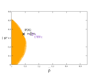
Figure 3: The theoretical values of the model III at $90\%$ CL in the $\bar{\rho}{\bf-}\bar{\eta}$ plane . Two experimental values (5) and (6) are also plotted. The best fit point is denoted as $\times$.

By making an overall $45^{\circ}$ rotation of the $Q_{6}$ doublets $Q,U^{c}$ and $D^{c}$ in the space of the family group, we obtain nearest neighbor interaction (NNI) type mass matrices:

$$M_{u}=\left(\begin{array}[]{ccc}0&c_{u}&0\\ -c_{u}&0&b_{u}\\ 0&d_{u}&e_{u}\end{array}\right)~{},~{}M_{d}=\left(\begin{array}[]{ccc}0&c_{d}&0\\ -c_{d}&0&b_{d}\\ 0&d_{d}&e_{d}\end{array}\right)\ .$$ (63)

All the elements of these matrices can be made real by a suitable redefinition of the quark fields. Then the real matrices can be diagonalized by orthogonal matrices as

$$O_{u}^{T}M_{u}M_{u}^{T}O_{u}={\rm diag}(m_{u}^{2},m_{c}^{2},m_{t}^{2}),$$ (64)

$$O_{d}^{T}M_{d}M_{d}^{T}O_{d}={\rm diag}(m_{d}^{2},m_{s}^{2},m_{b}^{2}),$$ (65)

and the CKM matrix takes the form

$$V=O_{u}^{T}PO_{d},$$ (66)

where $P={\rm diag}(1,e^{2i\theta},e^{i\theta})$. The phase rotation matrix $P$ has only one angle $\theta$, which is the consequence of a spontaneously and softly broken CP.

The full nine dimensional space of the parameters can be divided into two non-equivalent regions. The difference between the two regions, the region III and IV, can be reduced to the sign of $c_{d}$, so that without loss of generality the other parameters, i.e. $b_{u},c_{u}\dots,e_{d}$ in (63), can be assumed to be positive real numbers. (The parameter space for the model IV has not been considered in Babu:2004tn .) Accordingly, we define two models; the model III for positive $c_{d}$ and IV for negative $c_{d}$.

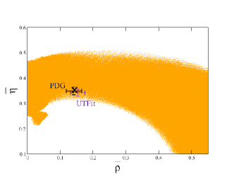
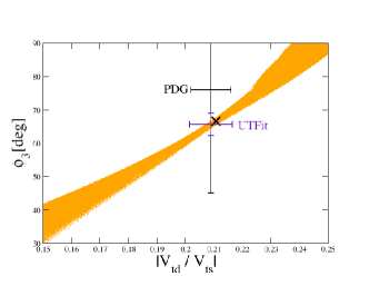
Figure 4: The theoretical values of the model IV at $90\%$ CL in the $\bar{\rho}{\bf-}\bar{\eta}$ plane (left) and $|V_{td}/V_{ts}|{\bf-}\phi_{3}(\gamma)$ plane (right). Two experimental values (5) and (6) are also plotted. The best fit point is denoted as $\times$.

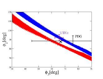
Figure 5: The theoretical values of the model IV at $90\%$ CL in the $\phi_{3}(\gamma){\bf-}\phi_{2}(\alpha)$ plane, where two predicted regions for $m_{s}/m_{b}=0.0220\pm 0.0007$ and $m_{d}/m_{b}=(1.200\pm 0.028)10^{-3}$ (red) and for $m_{s}/m_{b}=0.0170\pm 0.0007$ and $m_{d}/m_{b}=(0.930\pm 0.028)10^{-3}$ (blue) are plotted. Two experimental values (5) and (6) are also plotted. The best fit point is denoted as $\times$.

According to Harayama:1996jr , the CKM matrix can be approximately written in a closed form. One finds, for instance,

$$V_{us} \simeq -y_{d}\sqrt{\frac{m_{d}}{m_{s}}}+y_{u}\sqrt{\frac{m_{u}}{m_{c}}}\ e^{2i\theta}\ ,$$ (67)

$$V_{cb} \simeq \frac{y_{d}^{2}}{\sqrt{1-y_{d}^{4}}}\frac{m_{s}}{m_{b}}\ e^{2i\theta}-\frac{y_{u}^{2}}{\sqrt{1-y_{u}^{4}}}\frac{m_{c}}{m_{t}}\ e^{i\theta},$$ (68)

$$V_{ub} \simeq \frac{\sqrt{1-y_{d}^{4}}}{y_{d}}\sqrt{\frac{m_{d}}{m_{s}}}\frac{m_{s}}{m_{b}}$$ (69)

$$+y_{u}\sqrt{\frac{m_{u}}{m_{c}}}\left(\frac{y_{d}^{2}}{\sqrt{1-y_{d}^{4}}}\frac{m_{s}}{m_{b}}\ e^{2i\theta}-\frac{1}{y_{u}^{2}\sqrt{1-y_{u}^{4}}}\frac{m_{c}}{m_{t}}\ e^{i\theta}\right)\ ,$$

where $y_{u}=1/c_{u}$ and $y_{d}=1/c_{d}$. For $y_{d}\simeq 1$ we can reproduce the classic relations of Gatto:1968ss ; Cabibbo:1968vn ; Fritzsch:1977za

$$|V_{us}| \simeq \sqrt{\frac{m_{d}}{m_{s}}}+O(m_{u}/m_{c}).$$ (70)

We have performed numerical analyses on the CKM parameters of the models in detail, some of which are presented in Figs. 3 -5, where Fig. 3 is that of the model III, and Figs. 4 and 5 are those of the model IV.

The best fit for the model III is given by

$$\sin 2\phi_{1}(\beta) = 0.664,~{}\phi_{2}(\alpha)=81.397^{\circ},~{}|V_{us}|=0.2250,~{}|V_{cb}|=0.0416,$$

$$m_{u}/m_{t} = 0.860\times 10^{-5},~{}m_{c}/m_{t}=0.375\times 10^{-2},$$ (71)

$$m_{d}/m_{b} = 1.065\times 10^{-3},~{}m_{s}/m_{b}=0.199\times 10^{-1}$$

with $\chi^{2}=2.68$ for the set of parameters $\sin 2\phi_{1}(\beta),\phi_{2}(\alpha),m_{u}/m_{t},m_{c}/m_{t},m_{d}/m_{b},m_{s}/m_{b},|V_{us}|,|V_{cb}|$. As we can see from Fig. 3, the model could be excluded; the PDG value in the $\bar{\rho}-\bar{\eta}$ plane Amsler:2008zz is about $2\sigma$ away from the theoretical values. A more precise experimental determination of $\phi_{2}(\alpha)$ will be more supporting the conclusion.

The model IV, on the other hand, seems to be consistent with the PDG values Amsler:2008zz as well as with the Utfit group values utfit . In Fig. 5 we plot two predicted regions for $m_{s}/m_{b}=0.0220\pm 0.0007~{},~{}m_{d}/m_{b}=(1.200\pm 0.028)10^{-3}$ (red) and $m_{s}/m_{b}=0.0170\pm 0.0007~{},~{}m_{d}/m_{b}=(0.930\pm 0.028)10^{-3}$ (blue), which should be compared with (2). We see that precise measurements of $\phi_{2}(\alpha)$ can distinguish the two regions. We also find that the smaller the $m_{s}$ is, the larger is $\phi_{2}(\alpha)$.

The best fit for the set of parameters of the model IV,
$\bar{\rho},\bar{\eta},m_{u}/m_{t},m_{c}/m_{t},m_{d}/m_{b},m_{s}/m_{b},|V_{us}|,|V_{cb}|$, is given by:

$$\bar{\rho} = 0.144,~{}\bar{\eta}=0.352,~{}|V_{us}|=0.2254,~{}|V_{cb}|=0.0411,$$

$$m_{u}/m_{t} = 0.704\times 10^{-5},~{}m_{c}/m_{t}=0.390\times 10^{-2},$$ (72)

$$m_{d}/m_{b} = 0.965\times 10^{-3},~{}m_{s}/m_{b}=0.177\times 10^{-1}$$

with $\chi^{2}=1.03$, and

$$\phi_{3}(\gamma) = 66.698^{\circ},~{}\phi_{2}(\alpha)=87.650^{\circ},~{}|V_{us}|=0.2254,~{}|V_{cb}|=0.0411,$$

$$m_{u}/m_{t} = 0.788\times 10^{-5},~{}m_{c}/m_{t}=0.390\times 10^{-2},$$ (73)

$$m_{d}/m_{b} = 1.075\times 10^{-3},~{}m_{s}/m_{b}=0.194\times 10^{-1}$$

with $\chi^{2}=0.44$ for the set of parameters $\phi_{3}(\gamma),\phi_{2}(\alpha),m_{u}/m_{t},m_{c}/m_{t},m_{d}/m_{b},m_{s}/m_{b},|V_{us}|,|V_{cb}|$.

V Conclusion

We have investigated four predictive flavor models that are based on a low-energy discrete family symmetry. Two of them may be excluded by the present precision of the measurements of the CKM parameters. The problem of the model I has been already pointed out in Lavoura:2005kx . For the model II a more precise determination of the quark masses is very crucial, especially the mass ratio $m_{s}/m_{d}$. We have found that the smaller the mass ratio is, the better is the chance for the model II. We have also found that to confirm or exclude the model IV, more precise determinations of $\phi_{3}(\gamma)$ and $\phi_{2}(\alpha)$ as well as of the quark masses are indispensable. The uncertainty in the strange quark mass should be less than a little more than $10\%$ to make it comparable with the assumed uncertainties of $\sim 1^{\circ}$ and $\sim 2^{\circ}$ in $\phi_{2}(\alpha)$ and $\phi_{3}(\gamma)$, respectively, at about 50 inverse atto barn achieved at a future B factory.

In this letter we have restricted ourselves to low-energy predictive models. There are also high-energy predictive models Ma:2005tr -Ishimori:2008fi , which will be the target of our future investigations.

Acknowledgments
We would like to thank Masashi Hazumi for instructive discussions and useful comments. This work is supported by the Grants-in-Aid for Scientific Research from the Japan Society for the Promotion of Science (# 18540257).

References

• (1) R. Gatto, G. Sartori and M. Tonin, Phys. Lett.  B 28 (1968) 128.
• (2) N. Cabibbo and L. Maiani, Phys. Lett.  B 28 (1968) 131.
• (3) H. Fritzsch, Phys. Lett.  B 70 (1977) 436.
• (4) L. J. Hall and A. Rasin, Phys. Lett.  B 315 (1993) 164 [arXiv:hep-ph/9303303].
• (5) R. G. Roberts, A. Romanino, G. G. Ross and L. Velasco-Sevilla, Nucl. Phys.  B 615 (2001) 358 [arXiv:hep-ph/0104088].
• (6) P. Ramond, R. G. Roberts and G. G. Ross, Nucl. Phys.  B 406 (1993) 19 [arXiv:hep-ph/9303320].
• (7) G. Altarelli, Lectures given at the Summer Institute 2007, Fuji-Yoshida, Japan, 3 -10 Aug. 2007, and arXiv:0711.0161 [hep-ph].
• (8) E. Ma, Lectures given at the Summer Institute 2004, Fuji-Yoshida, Japan, 12 -19 Aug. 2004, and arXiv:hep-ph/0409075.
• (9) C. S. Lam, Phys. Rev.  D 78 (2008) 073015 [arXiv:0809.1185 [hep-ph]]; Phys. Rev. Lett.  101 (2008) 121602 [arXiv:0804.2622 [hep-ph]].
• (10) H. Fritzsch and Z. z. Xing, Prog. Part. Nucl. Phys.  45 (2000) 1 [arXiv:hep-ph/9912358].
• (11) Y. Koide, Phys. Rev.  D 71 (2005) 016010 [arXiv:hep-ph/0406286].
• (12) S. Pakvasa and H. Sugawara, Phys. Lett.  B 73 (1978) 61; Phys. Lett.  B 82 (1979) 105.
• (13) E. Ma, Mod. Phys. Lett.  A 17 (2002) 627 [arXiv:hep-ph/0203238].
• (14) K. S. Babu, E. Ma and J. W. F. Valle, Phys. Lett.  B 552 (2003) 207 [arXiv:hep-ph/0206292].
• (15) Y. Koide, H. Nishiura, K. Matsuda, T. Kikuchi and T. Fukuyama, Phys. Rev.  D 66 (2002) 093006 [arXiv:hep-ph/0209333].
• (16) J. Kubo, A. Mondragon, M. Mondragon and E. Rodriguez-Jauregui, Prog. Theor. Phys.  109 (2003) 795 [Erratum-ibid.  114 (2005) 287] [arXiv:hep-ph/0302196].
• (17) J. Kubo, Phys. Lett.  B 578 (2004) 156 [Erratum-ibid.  B 619 (2005) 387] [arXiv:hep-ph/0309167].
• (18) Y. Koide, Phys. Rev.  D 69 (2004) 093001 [arXiv:hep-ph/0312207].
• (19) M. Frigerio, S. Kaneko, E. Ma and M. Tanimoto, Phys. Rev.  D 71 (2005) 011901 [arXiv:hep-ph/0409187].
• (20) K. S. Babu and J. Kubo, Phys. Rev.  D 71 (2005) 056006 [arXiv:hep-ph/0411226].
• (21) L. Lavoura and E. Ma, Mod. Phys. Lett.  A 20 (2005) 1217 [arXiv:hep-ph/0502181].
• (22) S. L. Chen and E. Ma, Phys. Lett.  B 620 (2005) 151 [arXiv:hep-ph/0505064].
• (23) T. Teshima, Phys. Rev.  D 73 (2006) 045019 [arXiv:hep-ph/0509094].
• (24) N. Haba and K. Yoshioka, Nucl. Phys.  B 739 (2006) 254 [arXiv:hep-ph/0511108].
• (25) E. Itou, Y. Kajiyama and J. Kubo, Nucl. Phys.  B 743 (2006) 74 [arXiv:hep-ph/0511268].
• (26) S. Morisi, arXiv:hep-ph/0604106.
• (27) C. Hagedorn, M. Lindner and F. Plentinger, Phys. Rev.  D 74 (2006) 025007 [arXiv:hep-ph/0604265].
• (28) E. Ma, H. Sawanaka and M. Tanimoto, Phys. Lett.  B 641 (2006) 301 [arXiv:hep-ph/0606103].
• (29) E. Ma, Mod. Phys. Lett.  A 21 (2006) 2931 [arXiv:hep-ph/0607190].
• (30) S. Kaneko, H. Sawanaka, T. Shingai, M. Tanimoto and K. Yoshioka, Prog. Theor. Phys.  117 (2007) 161 [arXiv:hep-ph/0609220].
• (31) F. Feruglio, C. Hagedorn, Y. Lin and L. Merlo, Nucl. Phys.  B 775 (2007) 120 [arXiv:hep-ph/0702194].
• (32) P. H. Frampton and T. W. Kephart, JHEP 0709 (2007) 110 [arXiv:0706.1186 [hep-ph]].
• (33) A. Blum, C. Hagedorn and M. Lindner, Phys. Rev.  D 77 (2008) 076004 [arXiv:0709.3450 [hep-ph]].
• (34) A. Blum, C. Hagedorn and A. Hohenegger, JHEP 0803 (2008) 070 [arXiv:0710.5061 [hep-ph]].
• (35) S. Sen, Phys. Rev.  D 76 (2007) 115020 [arXiv:0710.2734 [hep-ph]].
• (36) L. Lavoura and H. Kuhbock, Eur. Phys. J.  C 55 (2008) 303 [arXiv:0711.0670 [hep-ph]].
• (37) F. Feruglio and Y. Lin, Nucl. Phys.  B 800 (2008) 77 [arXiv:0712.1528 [hep-ph]].
• (38) P. H. Frampton and S. Matsuzaki, arXiv:0712.1544 [hep-ph].
• (39) S. Antusch, S. F. King and M. Malinsky, JHEP 0805 (2008) 066 [arXiv:0712.3759 [hep-ph]].
• (40) N. Kifune, J. Kubo and A. Lenz, Phys. Rev.  D 77 (2008) 076010 [arXiv:0712.0503 [hep-ph]].
• (41) H. Ishimori, T. Kobayashi, H. Okada, Y. Shimizu and M. Tanimoto, arXiv:0811.4683 [hep-ph].
• (42) A. Blum and C. Hagedorn, arXiv:0902.4885 [hep-ph].
• (43) E. Ma, Mod. Phys. Lett.  A 20 (2005) 2767 [arXiv:hep-ph/0506036].
• (44) C. Hagedorn, M. Lindner and R. N. Mohapatra, JHEP 0606 (2006) 042 [arXiv:hep-ph/0602244].
• (45) I. de Medeiros Varzielas, S. F. King and G. G. Ross, Phys. Lett.  B 648 (2007) 201 [arXiv:hep-ph/0607045].
• (46) Y. Cai and H. B. Yu, Phys. Rev.  D 74 (2006) 115005 [arXiv:hep-ph/0608022].
• (47) S. Morisi, M. Picariello and E. Torrente-Lujan, Phys. Rev.  D 75 (2007) 075015 [arXiv:hep-ph/0702034].
• (48) M. C. Chen and K. T. Mahanthappa, Phys. Lett.  B 652 (2007) 34 [arXiv:0705.0714 [hep-ph]].
• (49) M. C. Chen and K. T. Mahanthappa, arXiv:0710.2118 [hep-ph].
• (50) W. Grimus and H. Kuhbock, Phys. Rev.  D 77 (2008) 055008 [arXiv:0710.1585 [hep-ph]].
• (51) G. Altarelli, F. Feruglio and C. Hagedorn, JHEP 0803 (2008) 052 [arXiv:0802.0090 [hep-ph]].
• (52) F. Bazzocchi, S. Morisi, M. Picariello and E. Torrente-Lujan, arXiv:0802.1693 [hep-ph].
• (53) R. Howl and S. F. King, JHEP 0805 (2008) 008 [arXiv:0802.1909 [hep-ph]].
• (54) M. K. Parida, Phys. Rev. D 78 (2008) 053004 [arXiv:0804.4571 [hep-ph]].
• (55) H. Ishimori, Y. Shimizu and M. Tanimoto, arXiv:0812.5031 [hep-ph].
• (56) A. G. Akeroyd et al. [SuperKEKB Physics Working Group], arXiv:hep-ex/0406071.
• (57) T. Browder, M. Ciuchini, T. Gershon, M. Hazumi, T. Hurth, Y. Okada and A. Stocchi, JHEP 0802 (2008) 110 [arXiv:0710.3799 [hep-ph]].
• (58) T. Blum, T. Doi, M. Hayakawa, T. Izubuchi and N. Yamada, Phys. Rev.  D 76 (2007) 114508 [arXiv:0708.0484 [hep-lat]].
• (59) C. Amsler et al. [Particle Data Group], Phys. Lett.  B 667 (2008) 1.
• (60) H. D. Kim, S. Raby and L. Schradin, Phys. Rev.  D 69 (2004) 092002 [arXiv:hep-ph/0401169].
• (61) M. Bona et al. [UTfit Collabaration], http://www.utfit.org/
• (62) X. G. He and W. S. Hou, Phys. Rev.  D 41 (1990) 1517.
• (63) K. Harayama, N. Okamura, A. I. Sanda and Z. Z. Xing, Prog. Theor. Phys.  97 (1997) 781 [arXiv:hep-ph/9607461].
• (64) Z. z. Xing, H. Zhang and S. Zhou, Phys. Rev.  D 77 (2008) 113016 [arXiv:0712.1419 [hep-ph]].