Spatial motion of the Magellanic Clouds.
Tidal models ruled out?

Abstract

Recently, Kallivayalil et al. derived new values of the proper motion for the Large and Small Magellanic Clouds (LMC and SMC, respectively). The spatial velocities of both Clouds are unexpectedly higher than their previous values resulting from agreement between the available theoretical models of the Magellanic System and the observations of neutral hydrogen (H I) associated with the LMC and the SMC. Such proper motion estimates are likely to be at odds with the scenarios for creation of the large–scale structures in the Magellanic System suggested so far. We investigated this hypothesis for the pure tidal models, as they were the first ones devised to explain the evolution of the Magellanic System, and the tidal stripping is intrinsically involved in every model assuming the gravitational interaction. The parameter space for the Milky Way (MW)–LMC–SMC interaction was analyzed by a robust search algorithm (genetic algorithm) combined with a fast restricted N–body model of the interaction. Our method extended the known variety of evolutionary scenarios satisfying the observed kinematics and morphology of the Magellanic large–scale structures. Nevertheless, assuming the tidal interaction, no satisfactory reproduction of the H I data available for the Magellanic Clouds was achieved with the new proper motions. We conclude that for the proper motion data by Kallivayalil et al., within their 1–$\sigma$ errors, the dynamical evolution of the Magellanic System with the currently accepted total mass of the MW cannot be explained in the framework of pure tidal models. The optimal value for the western component of the LMC proper motion was found to be $\mu_{\mathrm{lmc}}^{\mathrm{W}}\gtrsim-1.3$ mas yr^-1 in case of tidal models. It corresponds to the reduction of the Kallivayalil et al. value for $\mu_{\mathrm{lmc}}^{\mathrm{W}}$ by $\approx$40% in its magnitude.

1 Introduction

The discussion of the origin and evolution of the Magellanic System has become very intense since the new proper motion data for the selected LMC/SMC stars were acquired by the Hubble Space Telescope (HST). The HST measurements yielded the new values for the mean proper motions of the Magellanic Clouds with an unprecedented accuracy (see Kallivayalil et al., 2006a, b). In comparison with the previous observational studies (e.g. Jones et al., 1994; Kroupa et al., 1994; Kroupa & Bastian, 1997), the corresponding measurement errors were reduced by a factor of 10. Even though the latest proper motion estimates are consistent with the previous observational results within the 1–$\sigma$ errors, their actual position in the velocity space of the Clouds is quite unexpected.

The current velocities of the LMC and the SMC are critical input parameters of any evolutionary model of the System. However, regarding the large heliocentric distance to the Magellanic Clouds, nobody attempted the observational determination of their proper motion until the papers by Jones et al. (1994) and Kroupa et al. (1994) were carried out. Some more studies have contributed to the research (e.g. Kroupa & Bastian, 1997; Drake et al., 2001; Pedreros et al., 2002) offering a span of the mean proper motion values, but reaching no substantial improvement in the measurement precision, that was still of the same order as the derived values themselves. Such errors admit a wide variety of scenarios for the interaction (Ruzicka et al., 2007), and make the observational estimates serve only as quite weak tests of the results based on the theoretical studies of the MW–LMC–SMC interaction (e.g. Lin & Lynden–Bell, 1982; Gardiner et al., 1994).

The theorists focusing on the evolutionary history of the Magellanic System have widely agreed on two basic physical processes dominating the formation of the Magellanic large–scale structures, including the Magellanic Stream, the Bridge and the Leading Arm (for details see Brüns et al., 2005). Those are the tidal fields and the ram pressure stripping.

The tidal origin of the extended Magellanic structures was investigated by Fujimoto & Sofue (1976), who assumed the LMC and the SMC to form a pair gravitationally bound for several Gyr, moving in a flattened MW halo. They identified some LMC and SMC orbital paths leading to the creation of a tidal tail. Lin & Lynden–Bell (1977) pointed out the problem of the large parameter space of the MW–LMC–SMC interaction. To reduce the size of the parameter space, they neglected both the SMC influence on the System and dynamical friction within the MW halo, and showed that such a configuration allows for the existence of a LMC trailing tidal stream. Following studies by Murai & Fujimoto (1980), Murai & Fujimoto (1984), Lin & Lynden–Bell (1982), Gardiner et al. (1994), or Lin et al. (1995) extended and developed tidal models of the MW–LMC–SMC interaction. Generally speaking, the tidal mechanism becomes efficient enough if the timescale for the interaction is several Gyr (Gardiner et al., 1994; Gardiner & Noguchi, 1996).

Meurer et al. (1985) involved continuous ram pressure stripping into their simulation of the Magellanic System. This approach was followed later by Sofue (1994) or by Moore & Davis (1994), who simplified the interaction between the LMC and the SMC, however. The Magellanic Stream was formed of the gas stripped from outer regions of the Clouds due to collisions with the MW extended ionized disk. Heller & Rohlfs (1994) argue for a LMC–SMC collision resulting into the gas distribution to the inter–cloud region where it was stripped off by ram pressure as the Clouds moved through the hot MW halo. Recently, Bekki & Chiba (2005) applied a complex gas–dynamical model including star–formation to investigate the dynamical and chemical evolution of the LMC. Mastropietro et al. (2005) introduced their model of the Magellanic System including hydrodynamics (SPH) and a full N–body description of gravity. They studied the interaction between the LMC and the MW. Neither Bekki & Chiba (2005) nor Mastropietro et al. (2005) considered the SMC gas in their models. However, it was shown that the Stream, which sufficiently reproduces the observed H I column density distribution, might have been created without the SMC gaseous component or even without the LMC–SMC interaction (Mastropietro et al., 2005). The history of the Leading Arm was not investigated.

In general, hydrodynamical models allow for a better reproduction of the H I column density profile of the Magellanic Stream than tidal schemes. However, they constantly fail to reproduce the Magellanic Stream radial velocity measurements and especially the high negative velocity tip of the Magellanic Stream. Both families of models suffer from serious difficulties when modeling the Leading Arm. Similar requirements as for the tidal models hold for the ram pressure stripping schemes concerning interaction timescales, unless the density of the extended gaseous halo of the MW is increased substantially over its observational estimates, amplifying the hydrodynamical interaction. The ram pressure force is proportional to $\upsilon^{2}$ (relative velocity of the interacting gaseous objects). Thus, the process of gas stripping becomes more efficient as the velocity increases. However, for finite–size objects, it is accompanied by shorter interaction timescales due to the reduced crossing time.

Here we came to the actual point of controversy related to the papers by Kallivayalil et al. (2006a, b): the HST proper motion values put the Clouds on highly eccentric (or even unbound) orbits around the Galaxy. Besla et al. (2007) analyzed the orbital motion of the LMC using the HST data and brought convincing arguments justifying the previous statement. Such a result may have serious consequences for the proposed formation mechanisms of the Magellanic System, since it strongly discriminates the tidal scenario and probably also the ram pressure–based models. To explain the evolution of the Magellanic System by either of the mentioned processes, the negative total energy of the Clouds on their orbits about the MW is needed, which corresponds to multiple perigalactic approaches over the Hubble time. It is highly desirable to verify the reliability of the available models of the MW–LMC–SMC interaction if the orbital angular momentum of the Clouds is as high as found by Kallivayalil et al. (2006a, b).

Our paper presents the results of the search of the parameter space for the MW–LMC–SMC interaction dominated by tides. The approach applied was introduced by Ruzicka et al. (2007) and is based on an evolutionary optimization of the model input according to its ability to reproduce the H I observations of the Magellanic System (Brüns et al., 2005). The predictions by Besla et al. (2007) and by many others regarding the insufficient performance of tidal models in case of the Kallivayalil et al. (2006a, b) proper motions can only be confirmed if the entire parameter space for the interaction is explored. The method of the automated search for good models by the genetic algorithms (GA) enabled us to perform such an analysis for the first time. In addition to the LMC/SMC velocity problem, we also intend to answer two more questions: Are all the studied parameters of the same importance for successful modeling the MW–LMC–SMC interaction? Does the evolution of the System show similar behavior over various scales in the parameter space?

2 Parameter space of the interaction

Our model is built in a galactocentric Cartesian frame, assuming the present position of the Sun $\mathbf{r}_{\odot}=(-8.5,0,0)$ kpc and its spatial velocity $\mathbf{\upsilon}_{\odot}=(10.0,225.2,7.2)$ km s^-1 (Dehnen & Binney, 1998). In total, our study involves over 20 independent parameters, including the initial conditions of the LMC and the SMC motion, their total masses, parameters of mass distribution, particle disk radii, and orientation angles, and also the MW dark matter halo flattening parameter. Some of the parameters were constrained by theoretical studies (including scale radii $\epsilon$ of the LMC/SMC halos, the Coulomb logarithm $\Lambda$ for the dynamical friction in the MW halo, and the halo flattening parameter $q$ for the model of the MW gravitational potential). Their mean values and searched errors were discussed in Ruzicka et al. (2007). This section focuses on the observationally estimated parameters of the MW–LMC–SMC interaction.

Figure 1 shows the current proper motion of the LMC and the SMC as estimated by various observational methods, together with the portion of the velocity space that we studied. For convenience, the proper motion vectors were decomposed into the northern ($\mu^{\mathrm{N}}$) and the western ($\mu^{\mathrm{W}}$) components (see Kallivayalil et al., 2006a). We included every case that is acceptable up to date. In case of the LMC proper motion, the measurements by Jones et al. (1994); Kroupa et al. (1994); Kroupa & Bastian (1997); Drake et al. (2001); Pedreros et al. (2002) and Kallivayalil et al. (2006a) were considered. The proper motion errors for the SMC are based on the results by Kroupa & Bastian (1997); Irwin (1999); Freire et al. (2003); Anderson & King (2004a, b) and Kallivayalil et al. (2006b).

Efficiency and reliability of the optimization method – genetic algorithms – always depend on the number of possible solutions, that is extremely high in case of the Magellanic parameter space. To resolve the difficulty we performed a two–level search. First, the full volume of the parameter space was explored (referred to as a ”global scale” hereafter) to obtain a low resolution information about the behavior of the tidal model for various combinations of the input parameters. Subsequently, we reduced the volume of the parameter space by a factor of $10^{4}$ (”local scale” hereafter) to study only the 1–$\sigma$ proper motion errors by Kallivayalil et al. (2006a, b) with high resolution. Finally, both searches were compared. The extended ranges of the LMC and the SMC proper motion were

$$\mu^{\mathrm{N}}_{\mathrm{lmc}} = \langle-0.50,+1.80\rangle\,\mathrm{mas\,yr^{-1}}$$ (1)

$$\mu^{\mathrm{W}}_{\mathrm{lmc}} = \langle-2.23,-0.70\rangle\,\mathrm{mas\,yr^{-1}}$$ (2)

$$\mu^{\mathrm{N}}_{\mathrm{smc}} = \langle-2.50,-0.46\rangle\,\mathrm{mas\,yr^{-1}}$$ (3)

$$\mu^{\mathrm{W}}_{\mathrm{smc}} = \langle-2.05,+0.00\rangle\,\mathrm{mas\,yr^{-1}}.$$ (4)

To perform the high–resolution search, the volume of the parameter space was reduced by adopting the proper motion values derived by Kallivayalil et al. (2006a, b):

$$\mu^{\mathrm{N}}_{\mathrm{lmc}} = \langle+0.39,+0.49\rangle\,\mathrm{mas\,yr^{-1}}$$ (5)

$$\mu^{\mathrm{W}}_{\mathrm{lmc}} = \langle-2.11,-1.95\rangle\,\mathrm{mas\,yr^{-1}}$$ (6)

$$\mu^{\mathrm{N}}_{\mathrm{smc}} = \langle-1.35,-0.99\rangle\,\mathrm{mas\,yr^{-1}}$$ (7)

$$\mu^{\mathrm{W}}_{\mathrm{smc}} = \langle-1.34,-0.98\rangle\,\mathrm{mas\,yr^{-1}}.$$ (8)

The above introduced proper motion space for the Magellanic Clouds is illustrated by Fig. 1.

Unlike the proper motion of the Clouds, their LSR radial velocities could be measured with high accuracy. Following van der Marel et al. (2002), we set $\upsilon^{\mathrm{rad}}_{\mathrm{lmc}}=262.2\pm 3.4$ km s^-1. The SMC radial velocity error was estimated by Harris & Zaritsky (2006) as $\upsilon^{\mathrm{rad}}_{\mathrm{smc}}=146.0\pm 0.6$ km s^-1.

The heliocentric position vector of the LMC was adopted from van der Marel et al. (2002), i.e. the equatorial coordinates are $(\alpha_{\mathrm{lmc}},\delta_{\mathrm{lmc}})=(81.90^{\circ}\pm 0.98^{\circ},-69.87^{\circ}\pm 0.41^{\circ})$, its distance modulus is ${(m-M)}_{\mathrm{lmc}}=18.5\pm 0.1$. The equatorial coordinates of the SMC were set to the ranges $(\alpha_{\mathrm{smc}},\delta_{\mathrm{smc}})=(13.2^{\circ}\pm 0.3^{\circ},-72.5^{\circ}\pm 0.3^{\circ})$ (see Stanimirović et al., 2004, and references therein). Van den Bergh (2000) provided a great compilation of various distance determinations for the SMC, and we used his resulting distance modulus ${(m-M)}_{\mathrm{smc}}=18.85\pm 0.10$.

Several observational determinations of the LMC disk plane orientation have been published so far (see, e.g. Lin et al., 1995). In our parameter study, the LMC inclination $i$ and position angle $p$ together with their errors agree with van der Marel et al. (2002), i.e. $i=34.7^{\circ}\pm 6.2^{\circ}$ and $p=129.9^{\circ}\pm 6.0^{\circ}$. As the SMC misses a well defined disk, the orientation and the position angle usually refer to the SMC ”bar” defined by Gardiner & Noguchi (1996). Based on the estimates by Van den Bergh (2000) or Stanimirović et al. (2004), we adopted the error ranges $i=60^{\circ}\pm 20^{\circ}$ and $p=45^{\circ}\pm 20^{\circ}$ for the SMC initial disk inclination and position angle, respectively.

Gardiner et al. (1994) analyzed the H I surface contour map of the Clouds to estimate the initial LMC and SMC disk radii $r^{\mathrm{disk}}_{\mathrm{lmc}}$ and $r^{\mathrm{disk}}_{\mathrm{smc}}$, respectively. Regarding the absence of a clearly defined disk of the SMC and possible significant mass redistribution in the Clouds during their evolution, the results require a careful treatment.

Current total masses $m_{\mathrm{lmc}}$ and $m_{\mathrm{smc}}$ follow the estimates by Van den Bergh (2000). The masses of the Clouds are functions of time and evolve due to the LMC–SMC exchange of matter, and as a consequence of the interaction between the Clouds and the MW. Our test–particle model does not allow for a reasonable treatment of a time–dependent mass–loss. Therefore, the masses of the Clouds are considered constant in time, and their initial values at the starting epoch of simulations are approximated by the current LMC and SMC masses.

The dynamics of the MW–LMC–SMC interaction is critically dependent on the density distribution and the total mass of the Galaxy. We model the MW by the simple axially symmetric logarithmic potential involving 3 parameters (Binney & Tremaine, 1987). Only the MW halo flattening $q$ was treated as a free parameter in this study, varying within the range $\langle 0.78,1.20\rangle$ (see also Ruzicka et al., 2007), and thus introducing a spread in the total mass of the Galaxy $m_{\mathrm{MW}}(q)=\langle 0.92,2.15\rangle\cdot 10^{12}$ M_⊙ within the radius of 200 kpc.

3 Methodology

We investigate the pure tidal models in this paper, as they were the first ones devised to explain the creation of the Magellanic Stream (Fujimoto & Sofue, 1976). Beside that, the tidal stripping is intrinsically involved in every model assuming the gravitational interaction. The model itself is an advanced version of the scheme by Fujimoto & Sofue (1976): it is a restricted N–body (i.e. test particle) code describing the gravitational interaction between the Galaxy and its dwarf companions. The potential of the MW is dominated by the flattened dark matter halo, and the dynamical friction is exerted on the Magellanic Clouds as they move through the halo. The LMC and the SMC are represented by Plummer spheres, initially surrounded by test–particle disks. For further details see Ruzicka et al. (2007).

3.1 Genetic algorithm search

As mentioned already, the search itself was performed by GAs that mimic the selection strategy of the natural evolution. Holland (1975) first proposed the application of such an approach on optimization problems in mathematics. Recently, performance of GAs was studied for galaxies in interaction (see Wahde, 1998; Theis, 1999). As an example, Theis & Kohle (2001) analyzed the parameter space of two observed interacting galaxies – NGC 4449 and DDO 125. GAs turned out to be very robust tools for such a task if the routine comparing the observational and modeled data is appropriately defined. The approach by Theis & Kohle (2001) was later adopted and improved in order to explore the interaction of the Magellanic Clouds and the Galaxy (Ruzicka et al., 2007). The comparison between the model and observations became more efficient by involving an explicit search for the structural shapes in the data. Also the significant system–specific features (such as a special geometry and kinematics) were taken into account, further improving the GA performance for exploration of the MW–LMC–SMC interaction. More detailed information is to be found in Sec. 3.2 of this paper.

3.2 Comparison between model and observations: the Fitness Function

The proposed automatic search of the parameter space is driven by the routine comparing the modeled and observed H I distribution in the Magellanic System (Brüns et al., 2005). The match is measured by the fitness function ($F$) which is, in fact, a function of all input parameters, since every parameter set determines the resulting simulated H I data–cube. The devised function $F$ returns a floating–point number between 0.0 (complete disagreement) and 1.0 (perfect match), and consists of three different comparisons, including search for structures and analysis of local kinematics.

Efficiency of the GA is critically dependent on the applied fitness function. Theis & Kohle (2001) proposed a generally applicable technique based on comparing the relative intensities of the corresponding pixels in the modeled and observed data–cubes. Such a fitness function was successfully used to analyze an interaction involving two galaxies (Theis & Kohle, 2001). The mentioned comparison scheme became one of the three components of the fitness function developed for this project. Both modeled and observed H I column density values are scaled relative to their maxima to introduce dimensionless quantities. Then, we get

$$F_{1}=\frac{1}{N_{\upsilon}\cdot N_{x}\cdot N_{y}}\sum\limits_{i=1}^{N_{\upsilon}}\sum\limits_{j=1}^{N_{y}}\sum\limits_{k=1}^{N_{x}}\frac{1}{1+\left|\sigma_{ijk}^{\mathrm{obs}}-\sigma_{ijk}^{\mathrm{mod}}\right|},$$ (9)

where $\sigma_{ijk}^{\mathrm{obs}}$, $\sigma_{ijk}^{\mathrm{mod}}$ are normalized column densities measured at the position [j, k] of the i–th velocity channel of the observed and modeled data, respectively. $N_{\upsilon}=32$ is the number of separate LSR radial velocity channels in our data. $(N_{x}\cdot N_{y})=(32\cdot 64)$ is the total number of positions on the plane of sky for which observed and modeled H I column density values are available.

Ruzicka et al. (2007) further tested the performance of GA for the problem of galactic interactions, and an additional comparison dealing with the whole data–cubes was devised. It combines the enhancement of structures in the data by their Fourier filtering with the subsequent check for empty/non–empty pixels in both data–cubes. The corresponding component of the fitness function is defined as follows:

$$F_{2}=\frac{\sum\limits_{i=1}^{N_{\upsilon}}\sum\limits_{j=1}^{N_{y}}\sum\limits_{k=1}^{N_{x}}\mathrm{pix}_{ijk}^{\mathrm{obs}}\cdot\mathrm{pix}_{ijk}^{\mathrm{mod}}}{\max\left(\sum\limits_{i=1}^{N_{\upsilon}}\sum\limits_{j=1}^{N_{y}}\sum\limits_{k=1}^{N_{x}}\mathrm{pix}_{ijk}^{\mathrm{obs}},\sum\limits_{i=1}^{N_{\upsilon}}\sum\limits_{j=1}^{N_{y}}\sum\limits_{k=1}^{N_{y}}\mathrm{pix}_{ijk}^{\mathrm{mod}}\right)},$$ (10)

where $\mathrm{pix}_{ijk}^{\mathrm{obs}}\in\{0,1\}$ and $\mathrm{pix}_{ijk}^{\mathrm{mod}}\in\{0,1\}$ indicate whether there is matter detected at the position [i, j, k] of the 3 D data on the observed and modeled Magellanic System, respectively.

Effectively, such a comparison is a measure for the agreement of the structural shape in the data. No attention is paid to specific H I column density values here. We only test whether both modeled and observed emission is present at the same pixel of the position–velocity space. Ruzicka et al. (2007) showed that the search for structures significantly improves the GA performance if the structures of interest occupy only a small fraction of the system’s entire data–cube ($<10$% in the case of the Magellanic Stream and the Leading Arm).

Ruzicka et al. (2007) also recommended and successfully applied a system–specific comparison. In case of the Magellanic Clouds, the very typical linear radial velocity profile of the Stream including its high negative velocity tip was considered important. The slope of the LSR radial velocity function is a very specific feature, especially strongly dependent on the features of the orbital motion of the Clouds. Then, the third $F$ component is defined as

$$F_{3}=\frac{1}{1+\left|\frac{\upsilon_{\mathrm{min}}^{\mathrm{obs}}-\upsilon_{\mathrm{min}}^{\mathrm{mod}}}{\upsilon_{\mathrm{min}}^{\mathrm{obs}}}\right|},$$ (11)

where $\mathrm{\upsilon_{min}^{obs}}$ and $\mathrm{\upsilon_{min}^{mod}}$ are the minima of the observed LSR radial velocity profile of the Magellanic Stream and its model, respectively. The resulting fitness function $F$ combines the above defined components in the following way:

$$F=F_{1}F_{2}F_{3}.$$ (12)

In principle, the GA is able to find the global maximum of $F$ (i.e. the best model over the studied parameter space), but such a process may be very time–consuming due to the possibly slow convergence of $F$ (see Holland, 1975; Goldberg, 1989). In order to overcome such a difficulty, we searched the parameter space repeatedly in a fixed number of optimization steps, i.e. generations of models, and collected 120 high–quality models for either global or local scale of the parameter space. Distribution of the 120 local peaks of $F$ helps to map the fitness function landscape but it does not allow for conclusions on the behavior of $F$ either outside or inside the volume populated by the localized models. Therefore, in the following paragraphs we intend to devise a reasonable method for the further analysis of the fitness function $F$.

At this point, the reader might ask why there is such an attention paid to the properties of the fitness function itself if it, in fact, does not seem to provide any physical information about the interacting system of the Galaxy and the Magellanic Clouds. Indeed, the function $F$ serves primarily as a driver to the GA engine. However, the search for good models of the observed Magellanic System is efficient only if relevant astrophysical data are supplied as the input to $F$. As already mentioned, our study deals with detailed morphological and kinematic information from the 21 cm survey by Brüns et al. (2005) and with the corresponding modeled data. The fitness function then makes a link between the observable data and the initial state of the Magellanic System. Here we came to the benefits of spending time on studying the function $F$: in principle, it allows for identification of all points/regions in the parameter space leading to reproduction of the observational data, and also an appropriate analysis of its behavior may evaluate sensitivity of the System to variations in different parameters, i.e. their importance to the evolution of the System.

The parameter space of the interacting Magellanic Clouds is very extended. Acquiring helpful information about the function $F$ is quite a demanding task, but we consider it feasible once the goals of such an analysis are properly defined. The investigation of the fitness function $F$ is supposed to help us to answer two questions already raised in Section 1: Are all the studied parameters of the same importance for the properties of $F$? Does $F$ of the system show similar behavior over various scales in the parameter space?

3.3 Application of the Fitness Function

As the first step towards better understanding of the fitness function, we studied the 1 D projections of $F$ to the plane of the j–th parameter

$$F^{i}(p_{j})\equiv f(p^{i}_{1},\ldots,p_{j},\ldots,p^{i}_{n}),$$ (13)

where ${p^{i}_{1},\ldots,p^{i}_{j-1},p^{i}_{j+1},\ldots,p^{i}_{n}}$ are the specific values of the parameters corresponding to the i–th GA fit (point in the parameter space) and the parameter $p_{j}$ is varied within a given range. To quantify the sensitivity of $F^{i}(p_{j})$ to changes in different variables (parameters) several functions were defined. First, we have

$$\Delta^{i}_{j}\equiv\frac{\Sigma_{j}^{i}}{\overline{F^{i}(p_{j})}},$$ (14)

which is the relative deviation of the 1 D projected fitness $F^{i}(p_{j})$ from its mean value $\overline{F^{i}(p_{j})}$ on the studied interval, where

$$\Sigma_{j}^{i}\equiv\sqrt{\frac{1}{N_{\mathrm{P}}}\sum\limits_{k=0}^{N_{\mathrm{P}}-1}(F^{i}(p_{j,k})-\overline{F^{i}(p_{j})})^{2}}$$ (15)

is the corresponding deviation from $\overline{F^{i}(p_{j})}$ expressed for $N_{\mathrm{P}}$ points $p_{j,k}$ of the projected function $F^{i}(p_{j})$. We also calculate the relative change in $F^{i}(p_{j})$ as

$$\Delta^{i}_{j,\mathrm{F}}\equiv\frac{1}{2}\frac{\max(F^{i}(p_{j}))-\min(F^{i}(p_{j}))}{\overline{F^{i}(p_{j})}}.$$ (16)

The behavior of $F$ is analyzed here in terms of its deviation from the reference levels, which are established by the mean values of the 1 D projections $\overline{F^{i}(p_{j})}$. We found such an approach particularly useful if one wishes to distinguish between the large–scale and localized significant changes in $F$.

Low values of both, $\Delta^{i}_{j}$ and $\Delta^{i}_{j,\mathrm{F}}$, indicate presence of a global plateau of $F^{i}(p_{j})$, and thus weak dependence of the system on the j–th parameter. If the corresponding $\Delta^{i}_{j,\mathrm{F}}$ is of a significantly higher value, local peaks (or wells) exist. Similarly, the overall considerable evolution of $F^{i}(p_{j})$ is revealed by high values of both $\Delta^{i}_{j}$ and $\Delta^{i}_{j,\mathrm{F}}$. In such a case additional information is provided by the ratio of the functions (14) and (16). As the ratio approaches unity, abrupt changes in $F^{i}(p_{j})$ are favored over its smooth and slow evolution.

The intention of this section is to apply the method for the fitness function analysis introduced in Sec. 3.2 to the Magellanic System. The functions $\Delta^{i}_{j}$ and $\Delta^{i}_{j,\mathrm{F}}$ are helpful if features and behavior of the fitness function $F$ are studied in the neighborhood of an arbitrary point in the parameter space. However, to answer the above raised questions, an approach somewhat less detailed is sufficient. We suggest to treat the functions $\Delta^{i}_{j}$ and $\Delta^{i}_{j,\mathrm{F}}$ statistically and to calculate their mean values $\Delta_{j}\equiv\overline{\Delta^{i}_{j}}$ and $\Delta_{j,\mathrm{F}}\equiv\overline{\Delta^{i}_{j,\mathrm{F}}}$ over all 120 GA fits for both global and local scale cases. The function $F$ may be characterized by significantly different values of $\Delta^{i}_{j}$ or $\Delta^{i}_{j,\mathrm{F}}$ depending on the selected point in the parameter space. But for now, we are particularly interested in general trends in the behavior of the fitness function (i.e. the behavior of our model for the interaction) that should be expected if one studies the impact of variations in a selected parameter. As we will learn later, the identified GA fits cover a large fraction of the total parameter space volume. This fact also justifies the proposed statistical treatment of the 1 D projections of the function $F$ in case the results apply on the entire parameter space.

4 Results

Regarding the immense difficulties accompanying the observational measurement of the proper motions in case of the Magellanic Clouds, the models of the MW–LMC–SMC interaction were used to draw conclusions on the motion of the Clouds (e.g. Fujimoto & Sofue, 1976; Gardiner et al., 1994; Heller & Rohlfs, 1994; Gardiner & Noguchi, 1996). The mentioned models preferred either the tidal or hydrodynamical interactions as the processes dominating the evolution of the Magellanic System. Generally speaking, the proposed formation mechanisms are not efficient enough unless the Clouds orbit around the Galaxy. Several perigalactic approaches of the Clouds are expected by the tidal models (Gardiner et al., 1994; Connors et al., 2005). Shorter timescales for the interaction may be sufficient within the ram pressure scenario (Heller & Rohlfs, 1994; Mastropietro et al., 2005). However, the proper motions by Kallivayalil et al. (2006a, b) lead to timescales further dramatically reduced, as the Clouds should be approaching the Galaxy for the first time (Besla et al., 2007). The research of the dynamical evolution of the Magellanic System is at the point where our theoretical understanding of the MW–LMC–SMC interaction is at odds with some critical observational constraints.

Ruzicka et al. (2007) realized that the previous attempts to model the Magellanic System always reduced the parameter and initial condition space for the interaction by additional assumptions, such as omitting the SMC, or adopting a special orbit for the LMC. However, the uniqueness of the models is unclear unless a systematic analysis of the entire parameter space compatible with the available observations is performed. The idea by Ruzicka et al. (2007) was justified as they used a tidal model of the interaction and reproduced the observed H I structures for remarkably different histories of the System. Such a complex approach requires a powerful search method. Ruzicka et al. (2007) resolved the difficulty by employing GAs as optimization tools characterized by reliability and low sensitivity to local extremes (Theis & Kohle, 2001). We adopted their approach to analyze the performance of pure tidal models in case of the Magellanic System assuming the LMC and the SMC proper motions by Kallivayalil et al. (2006a, b).

4.1 Parameter Dependence

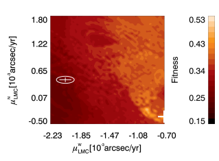
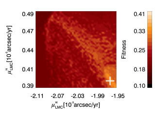
Figure 3: The ($\mu^{\mathrm{N}}_{\mathrm{lmc}}$, $\mu^{\mathrm{W}}_{\mathrm{lmc}}$)–planes for the 2 D projections of the function $F$. For the moment, the remaining parameters are fixed to the values corresponding to the best models for the original (upper plot) or the reduced proper motion ranges, respectively. The best models are marked by the white crosses. The white ellipse in the upper plot indicates the 68.3 % confidence region of the LMC proper motion by Kallivayalil et al. (2006a) and roughly corresponds to the entire ($\mu^{\mathrm{N}}_{\mathrm{lmc}}$, $\mu^{\mathrm{W}}_{\mathrm{lmc}}$)–plane depicted in the lower plot.

The values of $\Delta_{j}$ and $\Delta_{j,\mathrm{F}}$ were calculated for the fitness function $F$ over both global and local scales of the parameter space. Table 1 presents the result in the descending order according to the value of the function $\Delta_{j}$. Following the previous explanation it is clear, that the order reveals the sensitivity of the fitness function to various parameters. At this point, we feel qualified to answer the first question raised in Sec. 3.2: the parameters are not of the same importance for the properties of $F$. Table 1 indicates that the sensitivity of the Magellanic System to the choice for the LMC/SMC proper motions is significantly higher than in case of any of the remaining parameters This conclusion is well illustrated by Figure 3 depicting the fitness landscape projected to the plane of the LMC proper motion components. The projection was made at the positions of the best GA fits found for the global and local scale cases, respectively.

Our analysis has shown the critical dependence of the evolution of the Magellanic System on the LMC and the SMC spatial velocities. The function $\Delta_{j,\mathrm{F}}$ is not only useful for the detailed analysis of the fitness function, but can also serve to estimate the typical overall change in the fitness value over the entire studied parameter range. The value of $\Delta_{j,\mathrm{F}}$ exceeds 0.15 for every LMC/SMC proper motion component on the global scale (Tab. 1). Regarding the definition by Eq. (16), the mentioned values multiplied by the factor of 2.0 tell us how much the 1 D fitness projections $F^{i}(p_{j})$ change typically compared to their mean values. As the usual mean value $\overline{F^{i}(p_{j})}$ equals to $\approx 0.3$, one may assume the global proper motion ranges given by Eq. (1) to (4) to derive the following estimated changes in the fitness of our models per the unit step in the proper motion value:

$$\Delta F(\mu^{\mathrm{N}}_{\mathrm{lmc}})/\Delta\mu^{\mathrm{N}}_{\mathrm{lmc}} \simeq 0.04\,\mathrm{mas^{-1}\,yr}$$ (17)

$$\Delta F(\mu^{\mathrm{W}}_{\mathrm{lmc}})/\Delta\mu^{\mathrm{W}}_{\mathrm{lmc}} \simeq 0.06\,\mathrm{mas^{-1}\,yr}$$ (18)

$$\Delta F(\mu^{\mathrm{N}}_{\mathrm{smc}})/\Delta\mu^{\mathrm{N}}_{\mathrm{smc}} \simeq 0.09\,\mathrm{mas^{-1}\,yr}$$ (19)

$$\Delta F(\mu^{\mathrm{W}}_{\mathrm{smc}})/\Delta\mu^{\mathrm{W}}_{\mathrm{smc}} \simeq 0.06\,\mathrm{mas^{-1}\,yr}$$ (20)

The above listed values should be treated very carefully, as they simplify the real behavior of the fitness function. The fact that the proper motion of the SMC is even more critical than that of the LMC indicates, that both Clouds serve as sources of matter for the Magellanic large scale structures, but the SMC contribution responds to the choice for the orbit more strongly. It is another nice illustration of how much information about the physical properties of the Magellanic System can be actually obtained from the fitness function.

The estimates given by the Eq. (17) to (20) give a hint at the relation between the fitness and the physical properties of our models. Later in Sec. 4.3 the lower limit for the fitness of the satisfactory models will be established and discussed. While the best model we found yields $F_{\mathrm{best}}=0.514$, the fitness threshold level is $F_{\mathrm{lim}}>0.434$, i.e. all the acceptable models are found within the fitness range $(F_{\mathrm{best}}-F_{\mathrm{lim}})=0.08$. If any of the LMC/SMC proper motion components changes by 1 mas yr^-1, the corresponding model is extremely likely to cross the border between the successful and insufficient models. If some of the remaining parameters are altered by further observations, our findings concerning the motion of the Clouds shall not be affected strongly.

4.2 Scale Dependence

What if the volume of the parameter space is reduced substantially by changing the proper motion ranges of the Clouds? To find the answer, let’s take a look at Table 1. It indicates that the most influential parameters remain the same, if we zoom into the velocity space. The role of the choice for the LMC/SMC proper motion is still dominant for the evolution of the System. Impact of different proper motion components may be altered if their searched ranges are reduced. It is also a notable fact that the values of both functions $\Delta_{j}$ and $\Delta_{j,\mathrm{F}}$ decreased systematically over all studied parameters as we switched to the local scale of the parameter space. It means that the fitness function $F$ does not have a fractal–like (irregular) structure, and the probability of missing steep high peaks (i.e. isolated quality models) in the fitness landscape may be reduced by running the GA search again on that sub–region of the original parameter space, which is of a particular interest. We demonstrated that the effective resolution of the GA search may be improved by reducing the volume of the parameter space. Therefore, the exploration of the parameter space for the MW–LMC–SMC interaction was performed in two levels. First, every LMC/SMC proper motion estimate available was included. Subsequently, the proper motion spread was reduced to the 1–$\sigma$ error ranges by Kallivayalil et al. (2006a, b) to verify or eventually correct the global scale search.

4.3 Spatial motion and tidal models

We have analyzed the influence of the involved parameters on the tidal interaction in the Magellanic System. Reproduction of the H I observational data (Brüns et al., 2005) by the restricted N–body simulation turned out to be critically dependent on the current spatial velocities of the Clouds.

Since the effective resolution of the search can be improved by reducing the volume of the studied parameter space (as justified earlier in this section), two sets of the LMC/SMC proper motion ranges were assumed. After including every proper motion estimate available up to date, only the values by Kallivayalil et al. (2006a, b) were involved to allow for a high–resolution search on the local scale of the parameter space. With the use of GA, $\approx 2\cdot 10^{6}$ parameter combinations, i.e. individual N–body simulations, were tested in total, and 120 sets providing the highest fitness were collected for each of the studied volumes of the parameter space.

The resulting models are not considered acceptable unless they produce both leading and trailing H I Magellanic structures (the Leading Arm and the Magellanic Stream). Thus, to allow for quantitative statements, a threshold level of $F$ had to be established. In order to do so, one needs to understand how the modeled H I morphology and kinematics is reflected in the value of the fitness function.

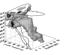
Figure 2: Visualization of the entire 3 D H I data–cube of the Magellanic System. The column density isosurface $\Sigma=10^{-5}\Sigma_{\mathrm{max}}$ is shown in every plot, together with the data–cubes projected to the 2 D maps of the integrated column density both in the position–position and position–radial velocity spaces. The best model ever found in the global scale search ($F=0.514$, $\mu_{\mathrm{lmc}}^{\mathrm{N}}=-0.34\,\mathrm{mas\,yr^{-1}}$, $\mu_{\mathrm{lmc}}^{\mathrm{W}}=-0.70\,\mathrm{mas\,yr^{-1}}$, left hand plot) is compared to the best model identified for the Kallivayalil et al. (2006a, b) data, i.e. the proper motion region delimited by Eq. (5) to (8), ($F=0.336$, $\mu_{\mathrm{lmc}}^{\mathrm{N}}=-1.96\,\mathrm{mas\,yr^{-1}}$, $\mu_{\mathrm{lmc}}^{\mathrm{W}}=+0.40\,\mathrm{mas\,yr^{-1}}$, right hand plot), and to the low–resolution compilation of the H I data by Brüns et al. (2005). The dashed line in the position–velocity projections depicts the mean radial velocity gradient along the observed Magellanic Stream.

The modeled distribution and kinematics of H I in the Leading Arm region and around the main LMC and SMC bodies remains similarly unsatisfactory over the entire parameter space, especially failing to reproduce the observed morphology of the Leading Arm (see Fig. 2). In terms of the fitness function, the value of $F$ never exceeds 0.3 if calculated only for the Leading Arm.

It is the Magellanic Stream that turned to be very sensitive to the choice for the model parameters, and critically influencing the resulting fitness. Figure 2 illustrates the above discussed facts. While the model of $F=0.514$ (global scale) is able to fit the basic features of the Magellanic Stream both in the projected H I distribution and the LSR radial velocity profile, the best model for the increased LMC/SMC spatial velocities ($F=0.336$, local scale) places the Magellanic Stream to the position–position–velocity space incorrectly, as the $\approx-400$ km s^-1 tip of the Stream is shifted towards the Clouds by $\approx 20^{\circ}$ compared to the observations (1 pixel in Fig. 2 equals roughly to $2^{\circ}$ in the plane of sky), and the modeled morphology differs seriously from the observed structure of the Magellanic Stream. Generally speaking, the described behavior of the modeled trailing stream is responsible for the resulting fitness of a given model, and was used to define the desired threshold level of the $F$ value.

Unlike the local scale analysis, the global search of the entire parameter space always resulted in a model placing the high negative radial velocity tip of the Stream to the correct projected position, and the modeled trailing stream filled roughly the same area of the H I data–cube as the observed Magellanic Stream. Following the mentioned fact, we selected the worst of the 120 fits from the global scale search to represent the threshold level of the fitness and so $F>0.434$ defines satisfactory models of the Magellanic System.

Figure 3 indicates, that the sub–region of the ($\mu_{\mathrm{lmc}}^{\mathrm{N}}$, $\mu_{\mathrm{lmc}}^{\mathrm{W}}$)–plane introduced by Kallivayalil et al. (2006a) does not allow for any satisfactory models assuming the pure tidal interaction. Such a conclusion is also confirmed by the local scale search restricted to the HST proper motion data only (lower plot of Figure 3). Thus, Fig. 3 denotes that it is not possible to simulate the evolution of the Magellanic System by pure tidal models if the spatial velocity of the LMC is as high as predicted by Kallivayalil et al. (2006a). However, such a speculation can only be confirmed if the entire parameter space of the interaction is explored, as it is based on the behavior of the fitness function $F$ in the neighborhood of the selected point.

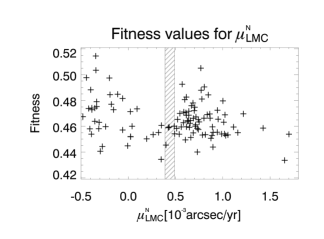
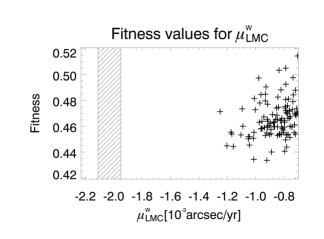
Figure 4: Distribution of all GA fits of the Magellanic System over the analyzed ranges for the LMC proper motion components $\mu^{\mathrm{N}}_{\mathrm{lmc}}$ and $\mu^{\mathrm{W}}_{\mathrm{lmc}}$. The upper row presents the low–resolution search of the original volume of the parameter space. The gray–filled areas indicate the reduced proper motion intervals. They were studied subsequently and the resulting span of the 120 identified GA fits is depicted in the lower row.

Figure 4 summarizes our results. The value of every local peak of the fitness function $F$ (i.e. the fitness of every model identified by GA) for the interaction of the MW–LMC–SMC system is plotted as function of the $\mu_{\mathrm{lmc}}^{\mathrm{N}}$ and $\mu_{\mathrm{lmc}}^{\mathrm{W}}$ proper motion components for the LMC. While the northern component $\mu_{\mathrm{lmc}}^{\mathrm{N}}$ allows for satisfactory modeling of the Magellanic System over the entire global range, the situation is quite different for the LMC proper motion in the western direction ($\mu_{\mathrm{lmc}}^{\mathrm{W}}$). The upper right plot of Figure 4 clearly indicates that the tidal scheme fails unless the $\mu_{\mathrm{lmc}}^{\mathrm{W}}$ values by Kallivayalil et al. (2006a) are reduced by $\approx 40$ % to reach $\mu_{\mathrm{lmc}}^{\mathrm{W}}\gtrsim-1.3$ mas yr^-1. Besla et al. (2007) have shown that the proper motion component $\mu_{\mathrm{lmc}}^{\mathrm{W}}$ controls the Galactocentric spatial velocity of the LMC. Hence, one can easily see that the pure tidal models of the Magellanic System constantly fail for the spatial velocities putting the LMC on highly eccentric or maybe unbound orbits about the Galaxy (Besla et al., 2007). This conclusion was verified and confirmed by the local scale parameter study focusing on the proper motion ranges by Kallivayalil et al. (2006a, b). Despite our efforts, no even decent models were found over this portion of the parameter space (see the lower row of Figure 4). Please note also that the concentration of the GA fits towards lower values of $\mu_{\mathrm{lmc}}^{\mathrm{W}}$ still remains even for the reduced velocity ranges.

Within the original volume of the parameter space, assuming the tidal interaction, no satisfactory reproduction of the H I data by Brüns et al. (2005) was achieved for the HST proper motions. In agreement with the previous studies, the model succeeded only if the Clouds were moving at substantially lower Galactocentric velocities. The following high–resolution analysis of the local scale of the parameter space (the proper motion ranges for the Clouds were restricted to the HST velocity data) did not change the previous result and no specific quality parameter combinations were revealed. Regarding the above summarized facts and results, we conclude that the dynamical evolution of the Magellanic System with the currently accepted total mass of the MW cannot be explained in the framework of pure tidal models for the proper motion data by Kallivayalil et al. (2006a, b) within their 1–$\sigma$ errors.

5 Conclusions

The new results introduced by Kallivayalil et al. (2006a, b) have serious consequences for our understanding of the dynamical evolution of the Magellanic System, and in a wider context they influence our view of the Local Group and its formation. Such facts, together with the key result of this paper indicating a conflict between the tidal models and observations of the Magellanic System, lead us necessarily to the questions about the reliability of the original HST data and correctness of their treatment by Kallivayalil et al. (2006a, b).

Unfortunately, the first issue cannot be addressed until the HST measurements are cross–checked by an instrument of a competitive resolution and other significant physical characteristics. In a close future, the GAIA mission should allow for high–precision astrometry, and hopefully the Magellanic Clouds and their proper motions will become objects of its interest as soon as possible.

Recently, an interesting constraint on the current velocity of the LMC was introduced by McClure–Griffiths et al. (2008). They were able to estimate the Galactocentric distance to the cross–section of the Magellanic Leading Arm with the gaseous disk of the MW. Although the observed part of the Leading Arm does not necessarily trace the future orbit of the LMC (the Leading Arm is believed to lead the Magellanic System), the measured position puts the lower limit on the Galactocentric distance to the point of the next passage of the LMC through the Galactic plane. Following McClure–Griffiths et al. (2008), the estimated distance is not at odds with the value obtained by adopting the current LMC velocity by Kallivayalil et al. (2006a). In addition to the above discussed issue, a verification of the distances to the main bodies of the Clouds may be worth a consideration. Space velocities also depend on the distances to the LMC/SMC, which should be checked carefully in future to clarify how far they may influence our conclusions.

Concerning the HST proper motion data processing by Kallivayalil et al. (2006a, b), both papers indicate that the data were analyzed and interpreted very carefully and the adopted method is well justified. A very strong support to the conclusions by Kallivayalil et al. (2006a, b) came recently from the study by Piatek et al. (2008) who also derived the LMC and the SMC current proper motions from the original HST data. Piatek et al. (2008) introduced a different method to process the LMC/SMC stellar proper motions, but their results agree with the findings by Kallivayalil et al. (2006a, b) very well. They were able to reduce the LMC/SMC proper motion errors by the factor of 3 compared to Kallivayalil et al. (2006a, b) due to their modified treatment of the original data. However, while their 1–$\sigma$ proper motion errors of the LMC are completely embedded within the corresponding error estimates by Kallivayalil et al. (2006a), the mean value of SMC proper motion component $\mu_{\mathrm{smc}}^{\mathrm{W}}$ is offset by +0.41 mas yr^-1 compared to Kallivayalil et al. (2006b) (see Fig. 1).

It means that the region of the parameter space delimited by the 1–$\sigma$ proper motion errors by Piatek et al. (2008) entered our global scale analysis, but it was not explored by the local scale search. Nevertheless, there is no indication that such a high–resolution exploration might alter significantly the results obtained for the global scale search. Since the only difference between the results by Kallivayalil et al. (2006a, b) and those by Piatek et al. (2008) exists for the western proper motion component of the SMC, the Eq. (20) yields a typical growth in the models’ fitness of $\Delta F(\mu^{\mathrm{W}}_{\mathrm{smc}})\approx+0.03$ as one switches from Kallivayalil et al. (2006a, b) to Piatek et al. (2008), because the $\mu_{\mathrm{smc}}^{\mathrm{W}}$ estimate by Piatek et al. (2008) is by $\approx 0.4$ mas yr^-1 lower than the result by Kallivayalil et al. (2006b). The overall quality of the models for the Piatek et al. (2008) data is then well below the fitness threshold level established in Sec. 4.3. Under such conditions it is extremely unlikely to expect any significant revision of the global scale parameter search by the high resolution analysis of the proper motions by Piatek et al. (2008).

If we admit that the latest observational estimates of the current proper motion for both Magellanic Clouds are correct, what would be the impact on our understanding of the Magellanic System and its evolution? We showed that the pure tidal stripping is insufficient to redistribute the H I gas in the System to conform the available observations (Brüns et al., 2005). Nevertheless, the classical model scheme by Fujimoto & Sofue (1976) offers an extremely simplified view of the physical processes influencing galactic interactions. Our results, together with the conclusions by Besla et al. (2007), do not allow for more than little doubts, that despite the high spatial velocities of the Clouds, the models of the interaction may succeed if sufficiently efficient physical mechanisms are introduced.

In the first order, the ram pressure stripping (Mastropietro et al., 2005) scenario is well worth further efforts, since its efficiency strongly depends on several only weakly constrained parameters, namely the density of the extended gaseous halo of the Galaxy. Moreover, the ram pressure force scales as $\upsilon^{2}$ with the relative velocity of the interacting objects, and so the high spatial velocities of the Clouds by Kallivayalil et al. (2006a, b) may compensate the effect of the corresponding reduced timescale for the interaction with the gaseous halo of the Galaxy. Recently, the paper by Nidever et al. (2008) offered an exciting alternative to the tidal/ram pressure models, considering the possible intense ejection of mass from several star–forming regions in the LMC super–shells.

Table 1: Parameter dependence of the fitness function

Global scale				Local scale
$j$	$\Delta_{j}\cdot 10^{2}$	$\Delta_{j,\mathrm{F}}\cdot 10^{2}$		$j$	$\Delta_{j}\cdot 10^{2}$	$\Delta_{j,\mathrm{F}}\cdot 10^{2}$
$\mu^{\mathrm{N}}_{\mathrm{smc}}$	15.96	31.03		$\mu^{\mathrm{N}}_{\mathrm{lmc}}$	3.09	5.53
$\mu^{\mathrm{W}}_{\mathrm{lmc}}$	8.76	17.20		$\mu^{\mathrm{N}}_{\mathrm{smc}}$	3.01	5.48
$\mu^{\mathrm{W}}_{\mathrm{smc}}$	8.55	18.92		$\mu^{\mathrm{W}}_{\mathrm{lmc}}$	2.64	4.85
$\mu^{\mathrm{N}}_{\mathrm{lmc}}$	6.98	15.24		$\mu^{\mathrm{W}}_{\mathrm{smc}}$	2.63	4.76
$\alpha_{\mathrm{lmc}}$	4.22	8.34		$\alpha_{\mathrm{lmc}}$	1.77	3.31
$(m-M)_{\mathrm{smc}}$	3.95	8.02		$R^{\mathrm{disk}}_{\mathrm{lmc}}$	1.69	2.94
$(m-M)_{\mathrm{lmc}}$	3.92	7.91		$M_{\mathrm{lmc}}$	1.69	3.11
$M_{\mathrm{lmc}}$	3.86	7.78		$\epsilon_{\mathrm{lmc}}$	1.67	3.09
$M_{\mathrm{smc}}$	3.48	6.93		$(m-M)_{\mathrm{lmc}}$	1.65	3.06
$\Lambda$	3.46	6.95		$\Lambda$	1.63	2.98
$\upsilon^{\mathrm{rad}}_{\mathrm{lmc}}$	3.31	6.52		$(m-M)_{\mathrm{smc}}$	1.59	2.95
$\epsilon_{\mathrm{lmc}}$	2.60	5.36		$M_{\mathrm{smc}}$	1.49	2.76
$\delta_{\mathrm{lmc}}$	2.38	4.69		$R^{\mathrm{disk}}_{\mathrm{smc}}$	1.47	2.64
$\epsilon_{\mathrm{smc}}$	2.23	4.62		$\upsilon^{\mathrm{rad}}_{\mathrm{lmc}}$	1.41	2.64
$\upsilon^{\mathrm{rad}}_{\mathrm{smc}}$	1.92	3.85		$\epsilon_{\mathrm{smc}}$	1.40	2.69
$\alpha_{\mathrm{smc}}$	1.91	3.89		$\delta_{\mathrm{lmc}}$	1.03	1.90
$i_{\mathrm{smc}}$	1.89	3.80		$p_{\mathrm{smc}}$	0.99	1.80
$\delta_{\mathrm{smc}}$	1.83	3.73		$i_{\mathrm{smc}}$	0.88	1.59
$p_{\mathrm{smc}}$	1.75	3.62		$\alpha_{\mathrm{smc}}$	0.88	1.59
$R^{\mathrm{disk}}_{\mathrm{lmc}}$	1.70	3.60		$\delta_{\mathrm{smc}}$	0.86	1.54
$R^{\mathrm{disk}}_{\mathrm{smc}}$	1.55	3.30		$\upsilon^{\mathrm{rad}}_{\mathrm{smc}}$	0.78	1.47
$i_{\mathrm{lmc}}$	0.70	1.39		$i_{\mathrm{lmc}}$	0.23	0.39
$p_{\mathrm{lmc}}$	0.64	1.29		$p_{\mathrm{lmc}}$	0.21	0.37

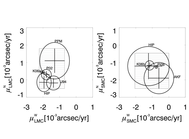
Figure 1: The 2 D projections of the Magellanic parameter space to the ($\mu^{\mathrm{N}}$, $\mu^{\mathrm{W}}$)–plane for both the LMC (left plot) and the SMC. The gray fillings mark the proper motion ranges explored by the GAs. The labels indicate the proper motions as expected by various studies. K06a stands for Kallivayalil et al. (2006a), K06b for Kallivayalil et al. (2006b), PI08 for Piatek et al. (2008), J94 for Jones et al. (1994), PPM for Kroupa et al. (1994), HIP for Kroupa & Bastian (1997), P02 for Pedreros et al. (2002), AKF for the value combining Freire et al. (2003) with Anderson & King (2004a, b). The ellipses show the 68.3 % confidence regions.

References

- Bekki & Chiba (2005) Bekki, K., & Chiba, M. 2005, MNRAS, 356, 680
- Anderson & King (2004a) Anderson, J., & King, I. R. 2004, ACS Instrument Science Report 04–15 (Baltimore: Space Telescope Science Institute)
- Anderson & King (2004b) Anderson, J., & King, I. R. 2004, AJ, 128, 950
- Besla et al. (2007) Besla, G., Kallivayalil, N., Hernquist, L., Robertson, B., Cox, T. J., van der Marel, R. P., & Alcock, C. 2007, ApJ, 668, 949
- Binney & Tremaine (1987) Binney, J., Tremaine, S. D. 1987, Galactic Dynamics (Princeton: Princeton University Press)
- Brüns et al. (2005) Brüns, C., Kerp, J., Staveley–Smith, L., et al., 2005, A&A, 432, 45
- Connors et al. (2005) Connors, T. W., Kawata, D., & Gibson, B. K. 2006, MNRAS, 371, 108
- Dehnen & Binney (1998) Dehnen, W., Binney, J. J. 1998, MNRAS, 298, 387
- Drake et al. (2001) Drake, A. J., Cook, K. H., Alcock, C., Axelrod, T. S., Geha, M., & MACHO Collaboration, 2001, BAAS, 33, 1379
- Freire et al. (2003) Freire, P. C., Camilo, F., Kramer, M., Lorimer, D. R., Lyne, A. G., Manchester, R. N., & D’Amico, N. 2003, MNRAS, 340, 1359
- Fujimoto & Sofue (1976) Fujimoto, M., & Sofue, Y. 1976, A&A, 47, 263
- Gardiner et al. (1994) Gardiner, L. T., Sawa, T., & Fujimoto, M. 1994, MNRAS, 266, 567
- Gardiner & Noguchi (1996) Gardiner, L. T., & Noguchi, M. 1996, MNRAS, 278, 191
- Goldberg (1989) Goldberg, D. E. 1989, Genetic algorithms in search, optimization and machine learning (New York: Addison–Wesley)
- Harris & Zaritsky (2006) Harris, J., Zaritsky, D. 2006, AJ, 131, 2514
- Heller & Rohlfs (1994) Heller, P., & Rohlfs, K. 1994, A&A, 291, 3, 743
- Holland (1975) Holland, J. H. 1975, Adaptation in natural and artificial systems. An introductory analysis with applications to biology, control and artificial intelligence (Ann Arbor: University of Michigan Press)
- Irwin (1999) Irwin, M. 1999, IAU Symposium 192, 409
- Jones et al. (1994) Jones, B. F., Klemola, A. R., & Lin, D. N. C. 1994, AJ, 107, 1333
- Kallivayalil et al. (2006a) Kallivayalil, N., van der Marel, R. P., Alcock, C., Axelrod, T., Cook, K. H., Drake, A. J., & Geha, M. 2006a, ApJ, 638, 772
- Kallivayalil et al. (2006b) Kallivayalil, N., van der Marel, R. P., & Alcock, C. 2006b, ApJ, 652, 1213
- Kroupa et al. (1994) Kroupa, P., Röser, S., & Bastian, U. 1994, MNRAS, 266, 412
- Kroupa & Bastian (1997) Kroupa, P., & Bastian, U. 1997, New A, 2, 77
- Lin & Lynden–Bell (1977) Lin, D. N. C., & Lynden–Bell, D. 1977, MNRAS, 181, 59
- Lin & Lynden–Bell (1982) Lin, D. N. C., & Lynden–Bell, D. 1982 , MNRAS, 198, 707
- Lin et al. (1995) Lin, D. N. C., Jones, B. F., & Klemola, A. R. 1995, ApJ, 439, 652
- van der Marel et al. (2002) van der Marel, R. P., Alves, D. R., Hardy, E., & Suntzeff, N. B. 2002, AJ, 124, 2639
- Mastropietro et al. (2005) Mastropietro, C., Moore, B., Mayer, L., et al. 2005, MNRAS, 363, 509
- McClure–Griffiths et al. (2008) McClure–Griffiths, N. M., Staveley–Smith, L., Lockman, Felix J., Calabretta, M. R., Ford, H. A., Kalberla, P. M. W., Murphy, T., Nakanishi, H., & Pisano, D. J. 2008, ApJ, 673, L143
- Meurer et al. (1985) Meurer, G. R., Bicknell, G. V., & Gingold, R. A. 1985, PASA, 6, 2, 195
- Moore & Davis (1994) Moore, B., & Davis, M. 1994, MNRAS, 270, 209
- Murai & Fujimoto (1980) Murai, T., & Fujimoto, M. 1980, PASJ, 32, 581
- Murai & Fujimoto (1984) Murai, T., & Fujimoto, M. 1984, Proceedings of the IAU Symposium No. 108, Dordrecht, D. Reidel Publishing Co., 115
- Nidever et al. (2008) Nidever, D. L., Majewski, S. R., & Butler B., W. 2008, ApJ, 679, 432
- Pedreros et al. (2002) Pedreros, M. H., Anguita, C., & Maza, J. 2002, AJ, 123, 1971
- Piatek et al. (2008) Piatek, S., Pryor, C., & Olszewski, E. W. 2008, AJ, 135, 1024
- Ruzicka et al. (2007) Ružička, A., Palouš, J., & Theis, C. 2007, A&A, 461, 155
- Sofue (1994) Sofue, Y. 1994, PASJ, 46, 4,431
- Stanimirović et al. (2004) Stanimirović, S., Staveley–Smith, L., Jones, P. A. 2004, ApJ, 604, 176
- Theis (1999) Theis, Ch 1999, RvMA, 12, 309
- Theis & Kohle (2001) Theis, Ch., & Kohle, S. 2001, A&A, 370, 365
- Van den Bergh (2000) Van den Bergh, S. 2000, The galaxies of the Local Group (Cambridge: Cambridge University Press)
- Wahde (1998) Wahde, M. 1998, A&A, 132, 417